Isotropic stars in higher-order torsion scalar theories

Gamal G.L. Nashed

Center for Theoretical Physics, British University in Egypt

Sherouk City 11837, P.O. Box 43, Egypt

e-mail:nashed@bue.edu.eg

Two tetrad spaces reproducing spherically symmetric spacetime are applied to the equations of motion of higher-order torsion theories. Assuming the existence of conformal Killing vector, two isotropic solutions are derived. We show that the first solution is not stable while the second one confirms a stable behavior. We also discuss the construction of the stellar model and show that one of our solution capable of such construction while the other cannot. Finally, we discuss the generalized Tolman-Oppenheimer-Volkoff and show that one of our models has a tendency to equilibrium.

1 Introduction

It is well known that in $f(T)$ gravity inflation [1] and late time cosmic acceleration can be realized in the early universe [2]–[27]. Recently there are many models constructed to describe dark energy without the use of cosmological constant (for more details see review [28] and references therein). The gravitational field equation of $f(T)$ gravity is second order as general relativity (GR). $f(T)$ gravity suffers from non-invariance of local Lorentz transformation [29]–[31], non-minimal coupling of teleparallel gravity to a scalar field [32]–[34] and non-linear causality [35]. Recently, number of $f(T)$ gravitational theories have been proposed [36]–[61]. The structures of neutron and quark stars in $f(T)$ theory have been discussed [62]. The anisotropic behavior, regularity conditions, stability and surface redshift of the compact stars have been checked [63]. Under those theories it is shown that $f(T)$ are not dynamically identical to teleparallel action plus a scalar field [60]. It has been shown that investigations of $f(T)$, using observational data, are compatible with observations (see e.g. [64, 65] and references therein). A new type of $f(T)$ theory was proposed in order to explain the acceleration phase of the universe [59]. Also it has been shown that the well-known problem of frame dependence and violation of local Lorentz invariance in the formulation of $f(T)$ gravity is a consequence of neglecting the role of spin connection [31].

$f(T)$ theory coupled with anisotropic fluid has been examined for static spacetimes with spherical symmetry and many classes of solutions have been derived [66]. It has been shown that some conditions on the coordinates, energy density and pressures, can produce new classes of anisotropic and isotropic solutions. Some of new black holes and wormholes solutions have been derived by selecting a set of non-diagonal tetrads [67]. It has been shown that relativistic stars can exist in $f(T)$ [68]. A special analytic vacuum spherically symmetric solution with constant torsion scalar, within the framework of $f(T)$, has been derived [69]. D-dimensional charged flat horizon solutions has been derived for a specific form of $f(T)$, i.e., $f(T)=T+\alpha T^{2}$ [70]. A complete investigation of the Noether symmetry approach in $f(T)$ gravity at FRW and spherical levels respectively has been investigated [71]. In the framework of $f(T)$ gravitational theories there are many solutions, spherically symmetric [58], spherically symmetric charged [73], homogenous anisotropic [74], stability of the Einstein static closed and open universe [75]. Some cosmological features of the $\Lambda$CDM model in the framework of the $f(T)$ are investigated [76]. However, till now, no spherically symmetric isotropic solution, using non-diagonal tetrad fields, derived in this theory. It is the aim of the present study to find an analytic, isotropic spherically symmetric solution in higher-order torsion scalar theories. The arrangement of this study are as follows: In Section §2, ingredients of $f(T)$ gravitational theory are provided. In Section §3, two different tetrad spaces having spherical symmetry are applied to the field equations of $f(T)$. Assuming the conformal Killing vector (CKV), we derived two non-vacuum spherically symmetric solutions in §3. The physics relevant to the derived solutions are analyzed in §4. The energy conditions are satisfied for the two solutions provided that the constants of integration be positive. In addition, the stability condition, the nature of the star and Tolman-Oppenheimer-Volkoff (TOV) equation are shown to be satisfied for one solution. The results obtained in this study are discussed in final section.

2 Ingredients of f(T) gravitational theory

Another description of Einstein’s general relativity (GR) of gravitation is done through the employ of what is called teleparallel equivalent of general relativity (TEGR). The ingredient quantity of this theory is the vierbein (tetrad) fields $\{h^{a}{{}_{\mu}}\}$ alternative to metric tensor fields $g_{\mu\nu}$. The associated metric $g_{\mu\nu}=\eta_{ab}h^{a}{{}_{\mu}}h^{b}{{}_{\nu}}$ with $\eta_{ab}=\textmd{diag}(1,-1,-1,-1)$ being Minkowskian metric, thus Levi-Civita symmetric connection $\mathring{\Gamma}^{\alpha}{{}_{\mu\nu}}$ is constructed from the metric and its first derivative [77]. Within TEGR, it is possible to build a nonsymmetric connection, Weitzenböck, $\Gamma^{\alpha}{{}_{\mu\nu}}=h^{a}{{}_{\mu}}\partial_{\nu}h_{a}{{}^{\alpha}}=-h_{a}{{}^{\alpha}}\partial_{\nu}h^{a}{{}_{\mu}}$. Tetrad space has a main merit that is the null of the vierbein’s derivative, i.e. $\nabla_{{}_{\nu}}h^{a}{{}_{\mu}}\equiv 0$, where $\nabla$, regarding the nonsymmetric Weitzenböck connection. Therefore, the vanishing of the vierbein’s covariant derivative recognizes auto-parallelism or absolute parallelism condition. Actually, the $\nabla$ operator is not invariant under local Lorentz transformations (LLT). The metric $g_{\mu\nu}$ is not able to guess one set of vierbein fields; thus extra freedom need to be determined so as to determine unique frame. Because of the absolute parallelism condition, it can be shown that the metricity condition is satisfied. The Weitzenböck connection is curvatureless while it has a non vanishing torsion tensor $T$ given as

$${T^{\lambda}}_{\mu\nu}:={h_{a}}^{\lambda}(\partial_{\mu}{h^{a}}_{\nu}-\partial_{\nu}{h^{a}}_{\mu}),$$ (2.1)

and contortion tensor $K$

$${K^{\mu\nu}}_{\alpha}=-\frac{1}{2}\left({T^{\mu\nu}}_{\alpha}-{T^{\nu\mu}}_{\alpha}-{T_{\alpha}}^{\mu\nu}\right).$$ (2.2)

The torsion scalar of TEGR theory is given by

$$\mathrm{T}:={T^{\alpha}}_{\mu\nu}{S_{\alpha}}^{\mu\nu},$$ (2.3)

with $S$ defined as

$${\mathrm{S}_{\alpha}}^{\mu\nu}:=\frac{1}{2}\left({\mathrm{K}^{\mu\nu}}_{\alpha}+\mathrm{\delta}^{\mu}_{\alpha}{\mathrm{T}^{\beta\nu}}_{\beta}-\mathrm{\delta}^{\nu}_{\alpha}{\mathrm{T}^{\beta\mu}}_{\beta}\right).$$ (2.4)

Equation (2.4) shows skewness in $\mu$ and $\nu$. Like $f(R)$, we could establish Lagrangian of $f(T)$ like

$${\mathcal{\mathrm{missing}}{L}}({\mathrm{h}^{a}}_{\mu},\mathrm{\Phi}_{A})=\int d^{4}xh\left[\frac{1}{16\pi}f(\mathrm{T})+{\mathcal{L}}_{Matter}(\mathrm{\Phi}_{A})\right],\quad\textrm{where}\quad\mathrm{h}=\mathrm{\sqrt{-g}}=det\left({\mathrm{h}^{a}}_{\mu}\right),$$

$$\mathrm{\Phi}_{A}\quad\textrm{are}\quad\textrm{ matter}\quad\textrm{fields}.$$ (2.5)

In this study we postulate the units in which $G=c=1$. Lagrangian (2) can consider as a function of the fields ${h^{a}}_{\mu}$. Variation of Lagrangian (2) with respect to the tetrad field ${h^{a}}_{\mu}$ we obtain the following field equations [36, 70]

$${S_{\mu}}^{\rho\nu}\,T_{,\rho}\ f(T)_{TT}+\left[h^{-1}{h^{a}}_{\mu}\partial_{\rho}\left(h{h_{a}}^{\alpha}{S_{\alpha}}^{\rho\nu}\right)-{T^{\alpha}}_{\lambda\mu}{S_{\alpha}}^{\nu\lambda}\right]f(T)_{T}-\frac{1}{4}\delta^{\nu}_{\mu}f(T)=-4\pi{\mathfrak{T}_{\mu}}^{\nu},$$ (2.6)

where $T_{,\rho}=\displaystyle\frac{\partial T}{\partial x^{\rho}}$,     $\mathrm{f(T)_{T}}=\displaystyle\frac{\partial\mathrm{f(T)}}{\partial T}$,    $\mathrm{f(T)_{TT}}=\displaystyle\frac{\partial^{2}\mathrm{f(T)}}{\partial T^{2}}$ and ${\mathfrak{T}_{\mu}}^{\nu}$ denotes the energy-momentum tensor of the anisotropic fluid which is defined as

$${\mathfrak{T}_{\mu}}^{\nu}=(\rho+p_{t})u_{\mu}u^{\nu}-p_{t}{\delta_{\mu}}^{\nu}+(p_{r}-p_{t})\eta_{\mu}\eta^{\nu},$$ (2.7)

with $p_{r}$ represents the radial pressure, $p_{t}$ the tangential pressure and

$$u_{\mu}u^{\mu}=-\eta_{\mu}\eta^{\mu}=1,\qquad{and}\qquad u^{\mu}\eta_{\mu}=0.$$ (2.8)

Equations (2.6) are the field equations of$f(T)$ gravitational theory.

3 Non-vacuum spherically symmetric solutions in higher-order torsion scalar theories

In this section, we are going to apply two, non-diagonal, different tetrad fields having spherical symmetry to the field equations (2.6).

3.1 First tetrad

The equation of motion of GR supply rich field to use symmetries which link geometry and matter in a natural way. Collineations are symmetries which come either from geometrical viewpoint or physical relevant quantities. The importance of collineations is the CKV which provides a more information of the construction of the spacetime geometry. The employs of the CKV simplifies the equations of motions of GR. The CKV is defined as

$${\mathbf{L}}_{\zeta}g_{ij}=\zeta_{i;j}+\zeta_{j;i}=\psi g_{ij},$$ (3.1)

with ${\mathbf{L}}$ being the Lie derivative and the $\psi$ being the conformal factor. One can assume the vector $\zeta$ which creates the conformal symmetry and makes the metric conformally mapped onto itself through $\zeta$. One must note that $\zeta$ and $\psi$ not necessary be static even supposing a static metric [78]. In addition, one must be careful about the following:
(i) if $\psi=0$, then (3.1) leads to a Killing vector,
(ii) if $\psi=constant$, then (3.1) leads to homothetic vector
(iii) if $\psi=\mathrm{\psi(x,t)}$ then (3.1) leads to conformal vectors. Furthermore, if $\psi$ is vanishing then the spacetime behaves as asymptotically flat and one has a null Weyl tensor. Thus, to have more understanding of the spacetime geometry one must take into account the CKV. Essentially, the Lie derivative ${\mathbf{L}}$ shows the inner field of gravity of a stellar configuration related to the vector field $\zeta$.

The first tetrad field having a spherical symmetry takes the shape [79]

$$\left({h^{i}}_{\mu}\right)=$$

,

(3.2)

where ${\mathcal{F}}_{1}(r)$, and ${\mathcal{F}}_{2}(r)$ are two unknown functions of the radial coordinate, $r$.

The associated metric of (3.2) takes the form

$$ds^{2}=-\frac{{{\mathcal{F}}_{1}}^{2}-{{\mathcal{F}}_{2}}^{2}}{{{\mathcal{F}}_{2}}^{2}}dt^{2}+({{\mathcal{F}}_{1}}^{2}-{{\mathcal{F}}_{2}}^{2})dr^{2}+d\Omega,\qquad d\Omega=r^{2}(d\theta^{2}+\sin^{2}\theta d\phi^{2}),$$ (3.3)

which is a static spherically symmetric spacetime admits one parameter group of conformal motion. Equation (3.3) is conformally mapped onto itself along $\zeta$. Therefore, (3.1) leads to

$$2[{\mathcal{F}^{\prime}}_{1}{{\mathcal{F}}_{1}}{{\mathcal{F}}_{2}}-{{\mathcal{F}}_{1}}^{2}{{\mathcal{F}^{\prime}}_{2}}]\zeta^{1}=\psi(r)[{{\mathcal{F}}_{1}}^{2}{\mathcal{F}}_{2}-{{\mathcal{F}}_{2}}^{3}],$$

$$\zeta^{0}=c,\qquad\qquad\qquad\zeta^{1}=\frac{\psi(r)r}{2},$$

$$2\zeta^{1}[{\mathcal{F}}_{1}{\mathcal{F}^{\prime}}_{1}-{\mathcal{F}}_{2}{\mathcal{F}^{\prime}}_{2}]+2\zeta^{\prime 1}[{{\mathcal{F}}_{1}}^{2}-{{\mathcal{F}}_{2}}^{2}]=\psi(r)[{{\mathcal{F}}_{1}}^{2}-{{\mathcal{F}}_{2}}^{2}],$$ (3.4)

where 0 and 1 refer to the temporal and spatial coordinates. Equation (3.1) leads to

$${\mathcal{F}}_{1}=\frac{\sqrt{1+{c_{0}}^{2}r^{2}}{\mathcal{F}}_{3}}{c_{0}r},\qquad{\mathcal{F}}_{2}=\frac{{\mathcal{F}}_{3}}{rc_{0}},\qquad\zeta^{i}=c_{1}{\delta^{i}}_{0}+\frac{\psi(r)r}{2}{\delta^{i}}_{1},\qquad{{\mathcal{F}}_{1}}\neq{{\mathcal{F}}_{2}},\qquad{{\mathcal{F}}_{3}}=\frac{c_{2}}{\psi(r)},$$ (3.5)

with $c$, $c_{0}$, $c_{1}$ and $c_{2}$ are constants of integration.

Using (3.5), tetrad (3.2) is rewritten as

$$\left({h^{i}}_{\mu}\right)=$$

,

(3.6)

Tetrad field (3.6) has the following associated metric

$$ds^{2}=-{c_{0}}^{2}r^{2}dt^{2}+{{\mathcal{F}}_{3}}^{2}dr^{2}+d\Omega,\qquad d\Omega=r^{2}(d\theta^{2}+\sin^{2}\theta d\phi^{2}),$$ (3.7)

Using (3.6) in (2.3) we get

$$\mathrm{T}=2\frac{2(1+2{c_{0}}^{2}r^{2}){\mathcal{F}}_{3}(r)-rc_{0}\sqrt{1+{c_{0}}^{2}r^{2}}(3+{{\mathcal{F}}_{3}}^{2}(r))}{c_{0}r^{3}\sqrt{1+{c_{0}}^{2}r^{2}}{{\mathcal{F}}_{3}}^{2}(r)},$$ (3.8)

Using Eqs. (3.8) and (3.6) in the field equations (2.6) we get the following non-vanishing components:

$$4\pi{{\mathcal{T}}_{0}}^{0}=4\pi\rho=-\frac{\sqrt{1+{c_{0}}^{2}r^{2}}{\mathcal{F}}_{3}-rc_{0}}{r^{2}c_{0}{{\mathcal{F}}_{3}}^{2}}T^{\prime}f_{TT}$$

$$+\frac{rc_{0}\sqrt{1+{c_{0}}^{2}r^{2}}(2{{\mathcal{F}}_{3}}-r{\mathcal{F}^{\prime}}_{3})-{{\mathcal{F}}_{3}}^{2}(1+2{c_{0}}^{2}r^{2})}{r^{3}c_{0}\sqrt{1+{c_{0}}^{2}r^{2}}{{\mathcal{F}}_{1}}^{3}}f_{T}+\frac{f}{4},$$

$$4\pi{{\mathcal{T}}_{1}}^{0}=-\frac{T^{\prime}f_{TT}}{r^{3}{c_{0}}^{2}},$$

$$-4\pi{{\mathcal{T}}_{1}}^{1}=4\pi p_{r}=-\frac{{{\mathcal{F}}_{3}}(1+2r^{2}{c_{0}}^{2})-3rc_{0}\sqrt{1+{c_{0}}^{2}r^{2}}}{r^{3}c_{0}{{\mathcal{F}}_{1}}^{2}\sqrt{1+{c_{0}}^{2}r^{2}}}f_{T}+\frac{f}{4},$$

$$-4\pi{{\mathcal{T}}_{2}}^{2}=-4\pi{{\mathcal{T}}_{3}}^{3}=4\pi p_{t}=-\frac{\sqrt{1+{c_{0}}^{2}r^{2}}{\mathcal{F}}_{3}-2rc_{0}}{2r^{2}c_{0}{{\mathcal{F}}_{3}}^{2}}T^{\prime}f_{TT}$$

$$+\frac{rc_{0}\sqrt{1+{c_{0}}^{2}r^{2}}({{\mathcal{F}}_{3}}^{3}+4{{\mathcal{F}}_{3}}-2r{\mathcal{F}^{\prime}}_{3})-2{{\mathcal{F}}_{3}}^{2}(1+2{c_{0}}^{2}r^{2})}{2r^{3}c_{0}\sqrt{1+{c_{0}}^{2}r^{2}}{{\mathcal{F}}_{3}}^{3}}f_{T}+\frac{f}{4}.$$ (3.9)

Second equation of (3.1) leads to $f_{TT}=0$, or $T=constant$. The case $T=constant$ gives a constant function and this is out the scope of the present study. Therefore, we seeking solutions make constrain on the form of $f(T)$ to have the form

$$f(T)=T,\qquad\quad\Rightarrow f_{TT}=0.$$ (3.10)

Assuming the isotropic condition

$$p_{r}=p_{t}=p,$$ (3.11)

and using (3.11) in (3.1), we get:

$${\mathcal{F}}_{3}(r)=\frac{2}{\sqrt{2+4r^{2}c_{3}}},$$

$$T=-\frac{6c_{3}c_{0}r^{3}\sqrt{1+r^{2}{c_{0}}^{2}}+5rc_{0}\sqrt{1+r^{2}{c_{0}}^{2}}-2(1+2{c_{0}}^{2}r^{2})\sqrt{2+4r^{2}{c_{3}}}}{r^{3}c_{0}\sqrt{1+r^{2}{c_{0}}^{2}}},$$

$$16\pi\rho=\frac{6c_{3}r^{2}-1}{r^{2}},\qquad 16\pi p=\frac{6c_{3}r^{2}+1}{r^{2}},\qquad\psi(r)=\frac{c_{2}\sqrt{2+4r^{2}c_{3}}}{2}.$$ (3.12)

The sound velocity ${v_{s}}^{2}$ is defined as ${v_{s}}^{2}:=\frac{dp}{d\rho}$. Using (3.1) we get the sound velocity in the form

$${v_{s}}^{2}=-1.$$ (3.13)

3.2 Second tetrad

The second tetrad space having a stationary and spherical symmetry takes the form [73]

$$\left({h^{i}}_{\mu}\right)=$$

,

(3.14)

where ${\mathcal{F}}_{4}(r)$ and ${\mathcal{F}}_{5}(r)$ are unknown functions. Using the same procedure applied to tetrad (3.2) we get the following equations of CKV of tetrad (3.14)

$$2{\mathcal{F}}^{\prime}_{4}\xi^{1}=\psi(r){\mathcal{F}}_{4},\qquad\xi^{0}=c,\qquad\xi^{1}=\frac{\psi(r)r}{2},\qquad 2\xi^{1}{\mathcal{F}}^{\prime}_{5}+2{\xi^{1}}_{,1}{\mathcal{F}}_{5}=\psi(r){\mathcal{F}}_{5},$$ (3.15)

The above set of equations imply

$${\mathcal{F}}_{4}=c_{4}r,\qquad{\mathcal{F}}_{5}=\frac{c_{5}}{\psi(r)},\qquad\xi^{i}=c_{6}{\delta^{i}}_{0}+\frac{\psi(r)r}{2}{\delta^{i}}_{1}.$$ (3.16)

where $c_{4}$, $c_{5}$ and $c_{6}$ are constants of integration .

Using (3.16), tetrad (3.14) can be rewritten as

$$\left({h^{i}}_{\mu}\right)=$$

.

(3.17)

Using (3.17), the torsion scalar (2.3), takes the form

$$T=\frac{2(3-4{\mathcal{F}}_{5}+{{\mathcal{F}}_{5}}^{2})}{r^{2}{{\mathcal{F}}_{5}}^{2}}.$$ (3.18)

Inserting (3.18) and the components of the tensors ${S^{\nu\mu}}_{\rho}$ and ${T^{\nu\mu}}_{\rho}$ in the field equations (2.6) we obtain

$$4\pi{{\mathcal{T}}_{0}}^{0}=4\pi\rho=\frac{(1-{{\mathcal{F}}_{5}})}{r{{\mathcal{F}}_{5}}^{2}}T^{\prime}f_{TT}-\frac{2{{\mathcal{F}}_{5}}^{2}-2{\mathcal{F}}_{5}+r{\mathcal{F}}^{\prime}_{5}}{r^{2}{{\mathcal{F}}_{5}}^{3}}f_{T}+\frac{f}{4},$$

$$-4\pi{{\mathcal{T}}_{1}}^{1}=4\pi p_{r}=\frac{3-2{\mathcal{F}}_{5}}{r^{2}{{\mathcal{F}}_{5}}^{2}}f_{T}+\frac{f}{4},$$

$$-8\pi{{\mathcal{T}}_{2}}^{2}=-8\pi{{\mathcal{T}}_{3}}^{3}=4\pi p_{t}=\frac{(2-{{\mathcal{F}}_{5}})}{2r{{\mathcal{F}}_{5}}^{2}}T^{\prime}f_{TT}-\frac{2{{\mathcal{F}}_{5}}^{2}-2{\mathcal{F}}_{5}+r{\mathcal{F}}^{\prime}_{5}-{{\mathcal{F}}_{5}}^{3}}{2r^{2}{{\mathcal{F}}_{5}}^{3}}f_{T}+\frac{f}{4},$$

The above system cannot be solved without assuming some a specific constraint on the form of $f(T)$. Therefore, we are going to use the constraint (3.10) in (3.2) and obtain the following

$${\mathcal{F}}_{5}(r)=\frac{2}{\sqrt{2+4r^{2}c_{7}}},$$

$$T=\frac{5\sqrt{2+4r^{2}c_{7}}-8-16r^{2}c_{5}+6c_{7}\sqrt{2+4r^{2}c_{7}}}{r^{2}\sqrt{2+4r^{2}c_{7}}},$$

$$16\pi\rho=\frac{9+18r^{2}c_{7}-8\sqrt{2+4r^{2}c_{7}}}{r^{2}},\qquad 16\pi p=\frac{11+18r^{2}c_{7}-8\sqrt{2+4r^{2}c_{7}}}{r^{2}},$$

$$\psi(r)=\frac{c_{5}\sqrt{2+4r^{2}c_{7}}}{2}.$$ (3.20)

Using (3.2), the sound velocity ${v_{s}}^{2}$ takes the form

$$\frac{dp}{d\rho}=\frac{16+32r^{4}{c_{7}}^{2}+48r^{2}c_{7}-22r^{2}c_{7}\sqrt{2+4r^{2}c_{7}}-11\sqrt{2+4r^{2}c_{7}}}{(8c_{7}\sqrt{2+4r^{2}c_{7}}-18r^{2}c_{7}-9+8\sqrt{2+4r^{2}c_{7}})\sqrt{2+4r^{2}c_{7}}}.$$ (3.21)

4 Physics relevant to the models

Energy conditions:
Energy conditions are essential tools to understand cosmology and general results related to strong gravitational fields. These tools are three energy conditions, null energy (NEC), the strong energy (SEC) and weak energy conditions (WEC) [80]–[82]. Such conditions have the following inequalities

$$NEC:\rho+p_{r}\geq 0,\qquad\rho+p_{t}\geq 0,$$

$$SEC:\rho+p_{r}\geq 0,\qquad\qquad\rho+p_{r}+2p_{t}\geq 0,$$

$$WEC:\rho\geq 0,\qquad\qquad\rho+p_{r}\geq 0,\qquad\qquad\rho+p_{t}\geq 0.$$ (4.1)

The broken of (4) leads to ghost instabilities.
Energy conditions of smooth transition models
Let us apply the above procedure of the energy conditions given by (4) to the derived solutions given in the previous section. For the case of isotropic, i.e., $p_{r}=p_{t}$, we can see from figures 1 and 2: The density has a positive value and the conditions $\rho+p\geq 0$ $\rho+3p\geq 0$ are satisfied when the constant $c_{3}>0$ for the first model and $c_{7}>0$ for the second model. This means that NEC, SEC and WEC conditions are satisfied for the above two models. Also it is interesting to note that the density and pressure of both solutions do not depend on the constants $c_{0}$ and $c_{4}$.

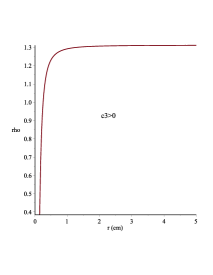
(a) $\rho$

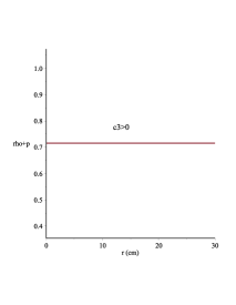
(b) $\rho$+p

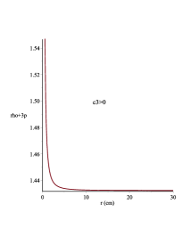
(c) $\rho$+3p

Figure 1: Energy conditions of the first model: The constant $c_{3}$ assumes a positive value so that the density be positive and also the pressure.

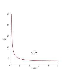
(a) $\rho$

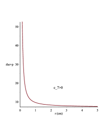
(b) $\rho$+p

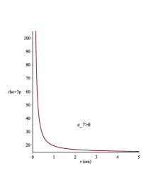
(c) $\rho$+3p

Figure 2: Energy conditions of the second model: The constant $c_{7}$ assumes a positive value so that the density be positive and also the pressure.

Stability problem
To study the stability issue of the above two models we use the cracking mechanism [83] in which the squared of speed sound must lies in the range [0,  1], i.e., $0\leq{v_{s}}^{2}\leq 1$. Figure 3 (a) does not show the positivity criterion i.e., ${v_{s}}^{2}\leq 0$. However, Fig. 3 (b) satisfies the criterion of stability i.e., ${v_{s}}^{2}\geq 0$ within the matter distribution provided any value of the constant $c_{7}$, in figure 3 (b), and thus second solution preserves stability.

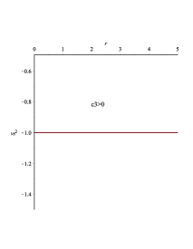
(a) ${v_{s}}^{2}<0$

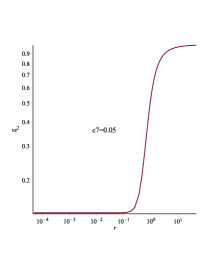
(b) ${v_{s}}^{2}\geq 0$

Figure 3: (a) shows that the first model does not has stability because the sound velocity ${v_{s}}^{2}\notin[0,1]$ as is required while (b) shows a stability behavior.

Nature of the star
To understand the star behavior we use a plot to indicate the radius of the stellar model for the second solution. Fig. 4, shows the cut on r-axis is approximately 1 km (Fig. 4). This value is a small value and shows a compact star [84, 85]. The value $R\sim 1$ km produces us to find the surface density of the system. As $r$ approximately vanishing, density approximates $\infty$ and thus, the central density is far from the aim of the present study. Only, we can inspect the surface density by close the values of the Newtonian constant, $G$, and the speed of light, $c$ in the expression of density which gives the numerical value as $13gm/cm^{3}$. This is a normal energy density in which the radius $R=1km$ is very small. This shows that the second solution of $f(T)$ describes an ultra-compact star [86]–[88]. The first model is not a physical one because to find the cutting of the pressure with the r-axis the constant $c_{3}<0$ which produces a contradiction with the energy conditions.

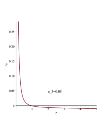
(a) p cut of the second model

Figure 4: The radius of star is shown when the pressure cuts r-axis.

TOV equation
The TOV equation has the shape

$$ds^{2}=-e^{\nu(r)}dt^{2}+e^{\lambda(r)}dr^{2}+r^{2}(d\theta^{2}+sin^{2}\theta d\phi^{2}),$$

can be written in the form [84]

$$-\frac{M_{G(r)}(\rho+p_{r})e^{\frac{\lambda(r)-\nu(r)}{2}}}{r^{2}}-\frac{dp_{r}}{dr}+\frac{2(p_{t}-p_{r})}{r}=0,$$ (4.2)

where $M_{G(r)}$ is mass of gravity in a sphere with radius $r$ which has the form

$$M_{G(r)}=\frac{r^{2}\nu^{\prime}e^{\frac{\lambda(r)-\nu(r)}{2}}}{2}.$$ (4.3)

Using (4.3) in (4.2), we obtain in the isotropic case

$$-\frac{\nu^{\prime}(\rho+p_{r})}{2}-\frac{dp_{r}}{dr}=0,$$ (4.4)

Equation (4.4) demonstrates the equilibrium of the configuration under distinct forces. As an equilibrium condition we write (4.4) in the form:

$$F_{g}+F_{h}=0,$$ (4.5)

where

$$F_{g}=-\frac{\nu^{\prime}(\rho+p_{r})}{2},\qquad\qquad F_{h}=-\frac{dp_{r}}{dr}.$$ (4.6)

Using (3.6), (3.1), (3.17) and (3.2) we plot the feature of TOV equation for the above two models in Figure 5.

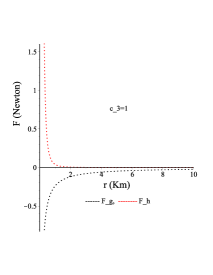
(a) TOV of the first model

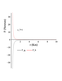
(b) TOV of the second model

Figure 5: Two distinct forces, i.e., $F_{g}$ and $F_{h}$ are schemed via r (km) for the two models.

5 Conclusion and discussion

In this study we have used two non diagonal different tetrad fields having spherical symmetry and reproduce the same associated metric. These tetrads are connected by local Lorentz transformation. We have used the CKV mechanism to reduce the highly nonlinear partial differential equations. We have applied the field equations of $f(T)$ to the first tetrad and have obtained anisotropic system consists of four non linear differential equations. One of these deferential equations put a constraint on the form of $f(T)$. This constraints make the form of $f(T)$ to be $f(T)=T$. Using this form and the isotropic condition, i.e., $p_{r}=p_{t}$, we get an isotropic solution.

For the second tetrad we have obtained anisotropic system that consists of three non linear differential equations. We cannot solve this system without any constrains on the form of $f(T)$. Using the constraint of $f(T)$ applied to the first tetrad, i.e. $f(T)=T$ and the condition of isotropy, we get another solution.

We have studied the physics relevant to each solution and have shown that the first and second tetrads satisfied the energy conditions provided that the two constants of integration involved in these solutions be positive. We have shown that the first tetrad is not stable one because the sound speed is negative, i.e., $\frac{dp}{d\rho}<0$ [83]. However, the second model has confirmed stable manner and has shown a dynamical behavior. We have indicated that the first tetrad is not suitable to construct a stellar model because the radius has an imaginary quantity. In meanwhile the second model has illustrated a stellar model that has a radius about one $Km$ and the density is not a dense on the surface. Finally we have shown that the figures of the widespread TOV equation indicate that static equilibrium has been achieved by distinct forces. Figure 5b show that the second model has a tendency toward equilibrium while the first one did not show such equilibrium.

References

• [1] R. Ferraro and F. Fiorini, Phys. Rev. D 75 (2007).
• [2] E. V. Linder, Phys. Rev. D 81 (2011), 127301.
• [3] P. Wu and H. W. Yu, Eur. Phys. J. C 71 (2011), 1552.
• [4] K. Bamba, C. Q. Geng, C. C. Lee and L. W. Luo, JCAP 1101 (2011), 021.
• [5] K. Bamba, S. D. Odintsov, D. S.-Gomez, Phys. Rev. D 88 (2013), 084042.
• [6] J. B. Dent, S. Dutta and E. N. Saridakis, JCAP 1101 (2011), 009.
• [7] K. Bamba, R. Myrzakulov, S. Nojiri and S. D. Odintsov, Phys. Rev. D 85 (2012), 104036.
• [8] A. Aviles, A. Bravetti, S. Capozziello and O. Luongo, Phys. Rev. D 87 (2013), 064025.
• [9] M. Jamil, D. Momeni and R. Myrzakulov, Eur. Phys. J. C 72 (2012), 2075.
• [10] M. Sharif and S. Rani, Astrophys. Space Sci. 345 (2013), 217.
• [11] R. Ferraro and F. Fiorini, Phys. Lett. B 702 (2011), 75.
• [12] R. Ferraro and F. Fiorini, Int. J. Mod. Phys. Conf. Ser. 3 (2011), 227.
• [13] P. Wu and H. W. Yu, Phys. Lett. B 693 (2010), 415.
• [14] I. G. Salako, M. E. Rodrigues, A. V. Kpadonou, M. J. S. Houndjo and J. Tossa, JCAP 060 (2013), 1475.
• [15] Z. Haghani, T. Harko, H. R. Sepangi and S. Shahidi, JCAP 1210 (2012), 061.
• [16] Z. Haghani, T. Harko, H. R. Sepangi and S. Shahidi, Phys. Rev. D 88 (2013), 044024.
• [17] T. Shirafuji and G. G. L. Nashed, Prog. Theor. Phys. 98 (1997), 1355.
• [18] K. Bamba, S. Nojiri and S. D. Odintsov, Phys. Lett. B 725 (2013), 368.
• [19] K. Bamba, J. de Haro and S. D. Odintsov, JCAP 1302 (2013), 008.
• [20] S. Nojiri and S. D. Odintsov, Phys. Rept. 505 (2011), 59.
• [21] G. G. L. Nashed, Int. J. Mod. Phys. A 21 (2006), 3181.
• [22] S. Nojiri and S. D. Odintsov, eConf C 0602061 (2006), 06.
• [23] S. Nojiri and S. D. Odintsov, Int. J. Geom. Meth. Mod. Phys. 4 (2007), 115.
• [24] S. Capozziello and V. Faraoni, Beyond Einstein Gravity (Springer, 2010); S. Capozziello and M. De Laurentis, Phys. Rept. 509 (2011), 167.
• [25] A. de la Cruz-Dombriz and D. Saez-Gomez, Entropy 14 (2012), 1717.
• [26] S. -H. Chen, J. B. Dent, S. Dutta and E. N. Saridakis, Phys. Rev. D 83 (2011), 023508.
• [27] Y. -P. Wu and C. -Q. Geng, JHEP 1211 (2012), 142.
• [28] K. Bamba, S. Capozziello, S. Nojiri, and S. D. Odintsov, Astrophysics and Space Science 342 (2012), 155.
• [29] B. Li, T. P. Sotirious and J. D. Barrow, Phys. Rev. D 83 (2011), 064035.
• [30] T. P. Sotirious, B. Li, J. D. Barrow, Phys. Rev. D 83 (2011), 104030.
• [31] M. KΕ‘Ε‘Γ‘rk, E. N. Saridakis, 1510.08432.
• [32] C. -Q. Geng, C. -C. Lee, E. N. Saridakis and Y. -P. Wu, Phys. Lett. B 704 (2011), 384.
• [33] C. -Q. Geng, J. -A. Gu and C. -C. Lee, Phys. Rev. D 88 (2013), 024030.
• [34] C. -Q. Geng, C. -C. Lee and E. N. Saridakis, JCAP 1201 (2012), 002.
• [35] Y. C. Ong, K. Izumi, J. M. Nester and P. Chen, Phys. Rev. D 88 (2013), 024019.
• [36] G. R. Bengochea and R. Ferraro, Phys. Rev. D 79 (2009), 124019.
• [37] C. Xu, E. N. Saridakis, and G. Leon, JCAP 1207 (2012), 005.
• [38] Y.-F. Cai, S.-H. Chen, J. B. Dent, S. Dutta, and E. N. Saridakis, Class. Quantum Grav. 28 (2011), 215011.
• [39] A. Einstein, Sitzungsber. Preuss. Akad. Wiss. Phys. Math. Kl., (1928) 217 (1930) 401.
• [40] J. Yang, Y.-L. Li, Y. Zhong and Y. Li, Phys. Rev. D 85 (2012), 084033.
• [41] K. Karami and A. Abdolmaleki, JCAP 04 (2012), 007.
• [42] G. G. L. Nashed, Eur. Phys. J. C 49 (2007), 851.
• [43] K. Atazadeh and F. Darabi, Eur. Phys. J. C 72 (2012), 2016.
• [44] H. Wei, X.-J. G. and L.-F. Wang, Phys. Lett. B 707 (2012), 298.
• [45] K. Karami, A. Abdolmaleki, Phys. Rev. D 88 (2013), 084034.
• [46] P. A. Gonzalez, E. N. Saridakis and Y. Vasquez, JHEP 2012 (2012), 53.
• [47] S. Capozziello, V. F. Cardone, H. Farajollahi and A. Ravanpak, Phys. Rev. D 84 (2011) 043527.
• [48] R.-X. Miao, M. Li and Y.-G. Miao, JCAP 2011 (2011), 033.
• [49] X.-H. Meng and Y.-B. Wang, Eur. Phys. J. C 71 (2011), 1755.
• [50] T. Shirafuji, G. G. L. Nashed and Y. Kobayashi, Prog. Theor. Phys. 96 (1996), 933.
• [51] H. Wei, X.-P. Ma and H.-Y. Qi, Phys. Lett. B 703 (2011),74.
• [52] M. Li, R.-X. Miao and Y.-G. Miao, JHEP 1107 (2011), 108.
• [53] S. Chattopadhyay and U. Debnath, Int. J. Mod. Phys. D 20 (2011), 1135.
• [54] P. B. Khatua, S. Chakraborty and U. Debnath, Int. J. Theor. Phys. 51 (2012), 405.
• [55] R.-J. Yang, Europhys. Lett. 93 (2011), 60001.
• [56] D. Liu and M. J. Reboucas, Phys. Rev. D 86 (2012) 083515.
• [57] K. Atazadeh, M. Mousavi, Eur. Phys. J. C 73 (2013), 2272.
• [58] G. G. L. Nashed, Eur. Phys. J. C 51 (2007), 377.
• [59] R.-J. Yang, Eur. Phys. J. C 71 (2011), 1.
• [60] R.-J. Yang, Eur. Phys. Lett. 93 (2011), 60001.
• [61] S. Nesseris, S. Basilakos, E. Saridakis, and L. Perivolaropoulos, Phys. Rev. D 88 (2013), 103010.
• [62] A. V. Kpadonou, M. J. S. Houndjo, M. E. Rodrigues, arXiv:1509.08771.
• [63] G. Abbas, A. Kanwal and M. Zubair, Astro. Phys. Space Sci. 357 (2015), 109.
• [64] R. Zheng and Q.-G. Huang, JCAP 1103 (2011), 002.
• [65] R. Ferraro and F. Fiorini, Int. J. Mod. Phys. Conf. Ser. 3 (2011), 227.
• [66] M. H. Daouda, M. E. Rodrigues and M. J. S. Houndjo, Eur. Phys. J. C 72 (2012) 1890.
• [67] M. H. Daouda, M. E. Rodrigues and M. J. S. Houndjo, Phys. Lett. B 715 (2012), 241.
• [68] C. G. BΓΆehmer, A. Mussa and N. Tamanini, Class. Quant. Grav. 28 (2011), 245020.
• [69] G. G. L. Nashed, Gen. Relat. Grav. 45 (2013), 1887.
• [70] S. Capozzielloa, P. A. GonzΓ‘lezc, E. N. Saridakise, Y. VΓ‘squez, JHEP 1302 (2013), 039.
• [71] A. Paliathanasis, S. Basilakos, E.N. Saridakis, S. Capozziello, K. Atazadeh, F. Darabi and M. Tsamparlis, Phys. Rev. D 89 (2014), 104042.
• [72] G. G. L. Nashed, Astrophysics and Space Science 330 (2010), 173.
• [73] G. G. L. Nashed Phys. Rev. D 88 (2013), 104034.
• [74] M. E. Rodrigues, M. J. S. Houndjo, D. SΓ‘ez-GΓ³mez and F. Rahaman, Phys. Rev. D 86 (2012), 104059.
• [75] J.-T. Li, C.-C. Lee and C.-Q. Geng, Eur. Phys. J. C73 (2013), 2315.
• [76] I. G. Salako, M. E. Rodrigues, A. V. Kpadonou. M. J. S. Houndjo and J. Tossa, JCAP 060 (2013), 1475.
• [77] C. W. Misner, K. S. Thorne and J. A. Wheeler, Gravitation (Freeman, San Francisco, 1973).
• [78] C. G. B$\ddot{o}$hmer, T. Harko and F. S. N. Lobo, Phys. Rev. D 76 (2007), 084014; Class. Quantum Gravit. 25 (2008), 075016.
• [79] G.G.L. Nashed, Gen. Relat. Grav. 34 (2002), 1047.
• [80] S. W. Hawking and G. E. R. Ellis, The Large Scale Structure of Spacetime. Cambridge University Press, Cambridge (1973).
• [81] S. Carroll, Spacetime and Geometry: An Introduction to General Relativity. Addison-Wesley, Reading (2004).
• [82] M. Zubair and S. Waheed, Astrophys. Space Sci. 355 (2015), 361.
• [83] L. Herrera, Phys. Lett. A 165 (1992), 206.
• [84] P. Bhar, F. Rahaman, S. Ray and V. Chatterjee, Eur. Phys. J. C 75 (2015), 190.
• [85] A. Das, F. Rahaman B. K. Guha, and S. Ray, Astrophys.Space Sci. 358 (2015), 36.
• [86] R. Ruderman, Rev. Astr. Astrophys. 10 (1972), 427.
• [87] N. K. Glendenning, Compact Stars: Nuclear Physics, Particle Physics and General Relativity (Springer-Verlag, New York, p. 70, 1997).
• [88] M. Herjog and F. K. Roepke, Phys. Rev. D84 (2011) 083002.