Propagation of radiation pulses through gas-plasma mixtures

Abstract

We determine the linear optical susceptibility of a radiation pulse propagating through a mixture of a gas of atoms or molecules and a plasma. For a specific range of radiation and plasma frequencies, resonant generation of volume plasmons significantly amplifies the radiation intensity. The conditions for resonant amplification are derived from the dispersion relations in the mixture, and the amplification is demonstrated in a numerical simulation of pulse propagation.

I Introduction

In applications of electromagnetic fields, radiation sometimes consists of a few photons only Chang et al. (2007) or interacts with a single molecule Nie and Emory (1997). As source and/or signal in such experiments are weak, it is necessary to amplify the interaction between matter and radiation. This has already been accomplished in a variety of ways Schmidt and Imamoǧlu (1996); Hau et al. (1999); Kang and Zhu (2003); Wang et al. (2006); Guerreiro et al. (2014), but a method that would target a specific spatial area in an adjustable way would be useful for designing experiments.

In recent years, a number of studies have addressed propagation of electromagnetic waves in an ultra-cold neutral plasma. Radio frequency fields have been used to study collective plasma electron oscillations and plasma expansion in ultra-cold neutral plasmas Kulin et al. (2000); Fletcher et al. (2006). In the optical regime these experiments are complemented by absorption imaging methods to determine the ion velocity distribution Simien et al. (2004); Killian et al. (2005). If radiation propagates through a gas of Rydberg atoms Mendonça et al. (2009) wave instabilities can occur due to energy transfer between excited Rydberg states and plasma electrons, and electrostatic waves Shukla (2010). Lu et al. Lu et al. (2011) suggested microwaves as a tool to measure the recombination rate of electrons and ions in ultra-cold neutral plasmas. Mendonça et al. Mendonça et al. (2010) predicted the generation of quasi-stationary magnetic fields by high-intensity radiation in Rydberg plasmas.

Radiation propagation through gas-plasma mixtures has also been studied for warm or hot plasmas. Plasma-induced optical sidebands around forbidden transitions in atomic spectra have been predicted Baranger and Mozer (1961) and demonstrated experimentally Kunze and Griem (1968); Cooper and Ringler (1969) long ago. During the past two decades, the focus has been on nonlinear effects induced by high-intensity radiation. Among the most interesting nonlinear phenomena in mixtures are relativistic guiding and self-modulation of short laser pulses Sprangle et al. (1990a, b, 1992); Esarey et al. (1994), harmonic generation and refraction Leemans et al. (1992); Mackinnon et al. (1996); Esarey et al. (1997), as well as de-focusing Sprangle et al. (1996) and dispersion Wu and Jr (2003). These effects are relevant to the construction of laser-driven plasma-based electron accelerators Esarey et al. (2009). Hu et al. Hu et al. (2005) predicted self-generation of a quasi-static magnetic field for short, intense laser pulses.

In this paper we determine under which conditions volume plasmons Xia et al. (2009) can be used to amplify a radiation pulse. Volume plasmons are electron density waves inside a plasma, which are related to surface plasmons at the interface between a metal and a dielectric. Our work is guided by the idea that the well-known method to amplify radiation using surface plasmons Lombardi and Birke (2012) may be extended to volume plasmons by employing a mixture of an atomic or molecular gas and plasma. The advantage of such a scheme would be that the amplification would not require the close (tens of nm) proximity of a metal surface. Furthermore, it would be possible to control the location where radiation is amplified, so that a specific set of molecules in a sample could be targeted. While we are mainly interested in the propagation of a controlled radiation pulse, our findings may also be of relevance for radiation propagation through the ionosphere or ionized interstellar media.

We derive an expression for the linear index of refraction for radiation propagating through the mixture. We show that a strong amplification may occur if volume plasmons are generated and demonstrate this effect by a numerical simulation of pulse propagation through the medium. Amplification is resonantly enhanced for specific radiation frequencies $\omega$ and angles $\theta$ between the radiation pulse and the velocity $\bm{v}_{\text{e}}$ of plasma electrons (see Fig. 1).

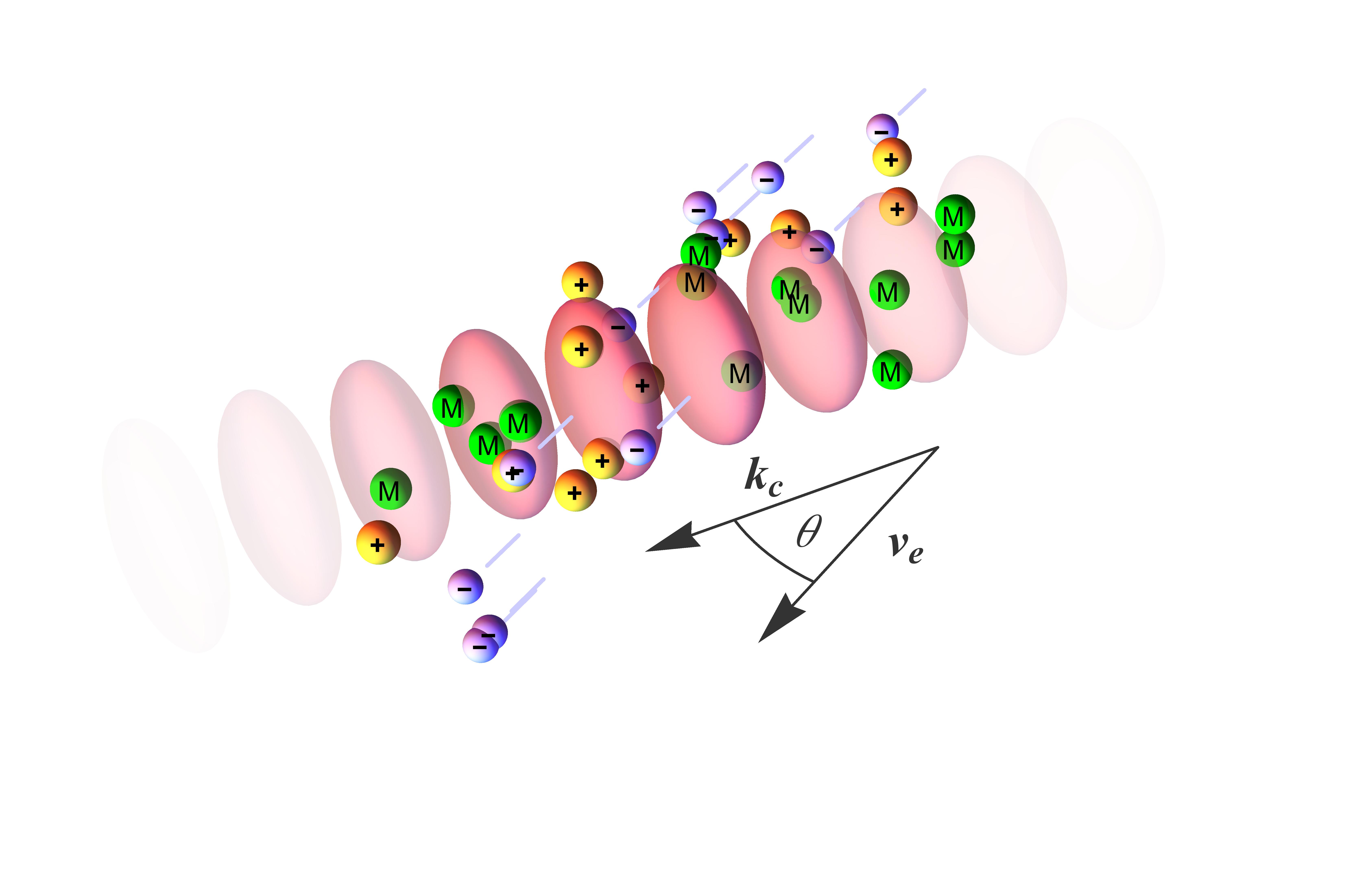
Figure 1: A radiation pulse (whose intensity maxima are represented by ellipses) with central wavevector $\bm{k}_{c}$ propagates through a mixture of a gas of atoms or molecules and a plasma. Molecules or atoms (M) and positive ions (+) are virtually immobile during the pulse propagation time. Plasma electrons (-) move with mean velocity $\bm{v}_{\text{e}}$ at an angle $\theta$ relative to the axis of the radiation pulse.

The paper is organized as follows. In Sec. II we discuss the general physical features of radiation-gas-plasma systems. Theoretical methods and results are summarized in Sec. III, followed by a detailed discussion of optical dispersion relations and field amplitudes in Sec. IV. Numerical results for pulse propagation through a mixture are presented in Sec. V. Several appendices contain the details of our calculations.

II Coupled radiation-atom-plasma systems

The physical case that we study is sketched in Fig. 1. A radiation pulse propagates through a mixture of an atomic gas and a plasma. For simplicity we refer to the gas particles as atoms, even though the gas may be composed of atoms or molecules. The plasma electrons move with (mean) velocity $\bm{v}_{\text{e}}$. To derive the linear optical susceptibility of this system and to simulate the propagation of a radiation pulse, we solve the coupled equations of motion for the radiation-atom-plasma system. In this section we describe the general features of these equations. Full details are given in App. A.

II.1 Plasma component

The plasma is modelled as a classical gas of ions and electrons, both of which may have a thermal distribution. For sufficiently short radiation pulses, the relatively slow motion of the ions may be neglected. The plasma dynamics can then be described by a phase-space distribution $f(\bm{r},\bm{p},t)$ of electrons. In the kinetic theory of electron gases, this distribution obeys a variant of the Boltzmann equation, which is called the Vlasov equation Sitenko and Malnev (1995). We use a relativistic generalization of the Vlasov equation Liboff (2003).

The Vlasov equation is non-linear in the dynamical fields, but for a weak radiation field it can be linearized in the deviation Goldston and Rutherford (1995)

$$\delta f(\bm{r},\bm{p},t)=f(\bm{r},\bm{p},t)-f_{0}(\bm{p}),$$ (1)

of $f(\bm{r},\bm{p},t)$ from the initial distribution $f_{0}(\bm{p})$, which is assumed to be spatially homogeneous. Our methods can be extended to spatially inhomogeneous initial distributions $f_{0}(\bm{r},\bm{p})$, but the required numerical resources are much larger than in the homogeneous case. The linearized relativistic Vlasov equation then takes the form

$$0 =\partial_{t}\delta f+\frac{1}{m\gamma}\bm{p}\cdot\nabla_{\bm{r}}\delta f-q\left(\bm{E}+\frac{1}{m\gamma}\bm{p}\times\bm{B}\right)\cdot\nabla_{\bm{p}}f_{0},$$ (2)

where $q$ and $m$ denote fundamental charge and electron mass, respectively. The last term describes the influence of the electromagnetic Lorentz force on the electrons, with $\gamma^{2}=1+(p/mc)^{2}$ the Lorentz factor.

II.2 Atomic gas

The detailed theory that is presented in App. A includes a full quantum field description of atomic observables, so that the methods developed here can be applied to molecular spectroscopy Lombardi and Birke (2008) and quantum information Ferguson et al. (2002); Schröder and Brown (2009); Soderberg et al. (2009). However, in this paper we focus on linear optical properties of atom-plasma mixtures, which are essentially of classical nature. We therefore describe the radiation field and plasma electrons using classical fields; only the internal (electronic) dynamics of atoms is treated quantum mechanically. The quantum nature of the atomic center-of-mass dynamics is only relevant at temperatures well below 1 mK Cohen-Tannoudji (1992), which is hard to realize even in ultracold atom-plasma mixtures. At temperatures above 1 mK, the center-of-mass motion can be included via Doppler broadening of spectral lines Cohen-Tannoudji et al. (2008).

Within this approximation, the atomic degrees of freedom can be described by a coherence field $\sigma_{ij}(\bm{r},t)$, which probes to what degree the atoms are prepared in a superposition of internal electronic states $|i\rangle$ and $|j\rangle$. In this work we focus on near-resonant electromagnetic fields, so that only the two atomic levels that are resonantly coupled need to be taken into account. We therefore can consider two-level atoms with ground state $|g\rangle$ and excited state $|e\rangle$. The polarization field is then related to the electromagnetic polarization field of the atomic gas through

$$\bm{P}(\bm{r},t)={\cal N}_{\text{{\tiny A}}}\bm{d}_{eg}\sigma_{eg}(\bm{r},t)+\text{ c.c.}\;,$$ (3)

with the atomic density ${\cal N}_{\text{{\tiny A}}}$. Here $\bm{d}_{eg}=\langle e|\hat{\bm{d}}|g\rangle$ is the atomic dipole moment, with $\hat{\bm{d}}$ the dipole operator. Hence, one may think of the coherence field as a re-scaled, complex form of the polarization field. Its equation of motion is derived in App. A and given by

$$\partial_{t}\sigma_{eg}(\bm{r},t) =\left(-i\omega_{0}-\frac{\Gamma}{2}\right)\sigma_{eg}(\bm{r},t)+\frac{i}{\hbar\varepsilon_{0}}\bm{D}_{\perp}(\bm{r},t)\cdot\bm{d}_{eg}^{\,*},$$ (4)

where $\omega_{0}$ denotes the atomic resonance frequency. The atomic spectral linewidth $\Gamma$ includes the effects of spontaneous emission as well as the influence of the environment, such as Doppler and collisional broadening. The field $\bm{D}_{\perp}(\bm{r},t)$ represents the transverse part ($\nabla\cdot\bm{D}_{\perp}=0$) of the electric displacement field $\bm{D}$.

II.3 Radiation Field

The radiation field is described using the macroscopic Maxwell equations

$$\nabla\cdot\bm{D} =\rho,$$ (5)

$$\nabla\cdot\bm{B} =0,$$ (6)

$$\nabla\times\bm{E} =-\partial_{t}\bm{B},$$ (7)

$$\nabla\times\bm{B} =\mu_{0}\left(\bm{J}+\partial_{t}\bm{D}\right),$$ (8)

with free charge density $\rho$ and free current density $\bm{J}$ provided by the plasma particles, and bound charges corresponding to the atoms. We assume that the magnetization field of the atom-plasma mixture is negligible. The atoms affect radiation through their polarization field $\bm{P}$, which appears in the material equation $\bm{D}=\varepsilon_{0}\bm{E}+\bm{P}$. To describe the interaction between atoms and a plane electromagnetic wave with wavevector $\bm{k}$ we introduce a set of basis vectors

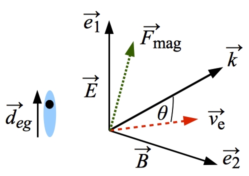
Figure 2: A radiation pulse with wavevector $\bm{k}$ is polarized in the direction of the dipole moment $\bm{d}_{eg}$ of the atoms. Depending on the direction of the plasma electron velocity $\bm{v}_{\text{e}}$, the magnetic force $\bm{F}_{\text{mag}}$ on the electrons can possess a component parallel to the wavevector.

$$\hat{\bm{k}}:=\frac{\bm{k}}{|\bm{k}|}\;,\;\bm{e}_{{1}}(\hat{\bm{k}})=\frac{\bm{d}_{\perp}(\hat{\bm{k}})}{\left|\bm{d}_{\perp}(\hat{\bm{k}})\right|}\;,\;\bm{e}_{{2}}(\hat{\bm{k}}) =\bm{e}_{{1}}^{*}(\hat{\bm{k}})\times\hat{\bm{k}},$$ (9)

where $\hat{\bm{k}}$ is a unit vector that is parallel to the wavevector and

$$\bm{d}_{\perp}(\hat{\bm{k}}):=\bm{d}_{eg}-\left(\hat{\bm{k}}\cdot\bm{d}_{eg}\right)\hat{\bm{k}}\;,$$ (10)

the part of $\bm{d}_{eg}$ that is perpendicular to $\hat{\bm{k}}$. For radiation polarized along $\bm{e}_{{1}}$, and the wavevector is perpendicular to $\bm{d}_{eg}$, the interaction between atoms and radiation is maximized. This situation is depicted in Fig. 2. If the polarization points along $\bm{e}_{{2}}$, the atoms appear transparent to the radiation pulse.

II.4 Volume plasmons

The interaction between plasma electrons and radiation enters into the Vlasov equation (2) through the Lorentz force $\bm{F}=-q\bm{E}-q\bm{v}_{\text{e}}\times\bm{B}$. In free space, electric and magnetic field amplitude of a radiation pulse are related through $\bm{B}=\hat{\bm{k}}\times\bm{E}/c$. For this reason, the magnetic force $\bm{F}_{\text{mag}}=-q\bm{v}_{\text{e}}\times\bm{B}$ is suppressed unless the electrons travel at relativistic speed. Hence, at low velocities, the electrons are only accelerated by the electric field in a direction perpendicular to the radiation pulse.

When $v_{\text{e}}$ is comparable to the speed of light $c$, the force $\bm{F}_{\text{mag}}$ cannot be neglected anymore. The fact that the magnetic force is always perpendicular to both $\bm{B}$ and $\bm{v}_{\text{e}}$ enables it to induce longitudinal modulations of the electron density, i.e., volume plasmons Xia et al. (2009), as long as the electron velocity is not exactly parallel to the wavevector. In Eq. (2), these modulations are generated by the term proportional to $\nabla_{\bm{p}}f_{0}$, which for a narrow momentum distribution is non-zero only for momenta $\bm{p}$ that are close to the initial mean momentum $\bm{p}_{e}$ of the electrons. This term acts as a source term for spatial variations, which are generated through the term involving $\nabla_{\bm{r}}\delta f$.

Plasmon generation can lead to dramatic changes of radiation dynamics, including amplification of light intensities near a metal surface by several orders of magnitude Kneipp et al. (2006). The discussion above suggests that the scenario depicted in Fig. 2 to generate volume plasmons inside an atom-plasma mixture will be most promising for light amplification. The radiation polarization is parallel to the atomic dipole moment, and plasma electrons move at relativistic speed with a velocity component along $\bm{e}_{{1}}$. The radiation pulse then interacts strongly with the atoms and can induce volume plasmons. If the electrons move in the direction of $\bm{e}_{{2}}$ instead, they could still form volume plasmons, but only for radiation that does not interact with atoms.

Plasma electrons with relativistic speed are not only interesting because of the increase of $\bm{F}_{\text{mag}}$, but also because they may interact resonantly with radiation. Generally, charged particles are most effectively accelerated if they move at the same speed as the phase front of an electromagnetic wave. In free space this is impossible, but in the presence of a dielectric medium with refractive index $n$, electrons are strongly interacting with radiation if their longitudinal velocity is $v_{\text{e}}=c/n$ Esarey et al. (2009).

In our case, this medium is formed by the atomic gas. Below we show that the absorption of radiation by atoms modifies the resonance condition $v_{\text{e}}=c/n$. A main result of our paper is to show that resonances can still occur, but only at specific optical frequencies, and for a specific range of electron densities.

III Theoretical Results

Solving the dynamics of radiation in an atom-plasma mixture is a lengthy and rather tedious process. In this section, we give a short summary of our methods and present the general results. The details of the derivation are presented in App. B.

The atom-plasma mixture is initially homogeneous, with the atoms prepared in their ground state. At time $t=0$, a weak radiation pulse with initial electric field amplitude $\bm{E}_{0}(\bm{r})$ is switched on. The dynamical equations of our system, Eqs. (2) for the plasmon dynamics, (4) for the atomic evolution, and the macroscopic Maxwell equations (5)-(8) for radiation propagation, all represent linear partial differential equations with constant coefficients in $t$ and $\bm{r}$.

To find the electric field amplitude $\bm{E}(\bm{r},t)$ at time $t>0$, we employ a spatial Fourier transform $\bm{r}\rightarrow\bm{k}$ and a temporal Laplace transform $t\rightarrow s$. This results in a set of algebraic equations that connect the Laplace-Fourier transform $\bm{E}(\bm{k},s)$ of the electric field with the transforms of all other dynamical fields. The solution takes the form

$$\bm{E}(\bm{k},s) =\bm{E}_{0}(\bm{k})\cdot\stackrel{{\scriptstyle\leftrightarrow}}{{R}}(\bm{k},s)\;,$$ (11)

with matrix $\stackrel{{\scriptstyle\leftrightarrow}}{{R}}(\bm{k},s)$ given in Eq. (63).

Solution (11) contains the complete information about the propagation of radiation through an atom-plasma mixture. Before studying the actual propagation in Sec. V we analyze the refractive index of the medium. The latter is usually represented as a complex function of the radiation frequency and can be derived from the roots of the denominator of Eq. (11); see Sec. IV. In order to accomplish this we make a variable substitution $s=-i\omega$. On the real axis, the (generally complex) variable $\omega$ can be interpreted as radiation frequency. The denominator of $\stackrel{{\scriptstyle\leftrightarrow}}{{R}}$ is then a function of $k$ and $\omega$. Solving for its roots $k(\omega)$ and employing the relation $k(\omega)=n(\omega)\omega/c$ would enable us to derive the refractive index $n(\omega)$ of the mixture. However, we prefer to use an equivalent approach, where $k=n\omega/c$ represents variable substitution, and then solve directly for the roots $n(\omega)$. Applying this variable substitution to $\stackrel{{\scriptstyle\leftrightarrow}}{{R}}$ yields

$$\stackrel{{\scriptstyle\leftrightarrow}}{{R}}\big{(}n,\omega,\hat{\bm{k}}\big{)} =-\stackrel{{\scriptstyle\leftrightarrow}}{{{\cal M}}}_{0}\cdot\Big{(}\omega^{2}(n_{\text{{\tiny A}}}^{2}-n^{2})\bm{e}_{{1}}^{\,*}\otimes\bm{e}_{{1}}+\omega^{2}(1-n^{2})\bm{e}_{{2}}^{\,*}\otimes\bm{e}_{{2}}+\stackrel{{\scriptstyle\leftrightarrow}}{{{\cal M}}}\Big{)}^{-1},$$ (12)

which is one of our main results. $n_{\text{{\tiny A}}}$ denotes the refractive index of the atomic gas in the absence of the plasma. For two-level systems, it is derived in App. B.1 and given by

$$n_{\text{{\tiny A}}}^{2}\big{(}\omega,\hat{\bm{k}}\big{)}=1-\frac{\eta\big{(}\hat{\bm{k}}\big{)}}{\omega-\omega_{0}+\eta\big{(}\hat{\bm{k}}\big{)}+i\frac{\Gamma}{2}}.$$ (13)

The parameter

$$\eta\big{(}\hat{\bm{k}}\big{)} :=\frac{{\cal N}_{\text{{\tiny A}}}}{\hbar\varepsilon_{0}}\bm{d}_{\perp}\big{(}\hat{\bm{k}}\big{)}\cdot\bm{d}_{eg}^{\,*}\;,$$ (14)

is related to the optical cooperativity parameter Fleischhauer and Yelin (1999). When $\eta\big{(}\hat{\bm{k}}\big{)}$ is significantly larger than the decoherence rate, the atomic density ${\cal N}_{\text{{\tiny A}}}$ is so large that the gas becomes opaque. The two matrices $\stackrel{{\scriptstyle\leftrightarrow}}{{{\cal M}}}$ and $\stackrel{{\scriptstyle\leftrightarrow}}{{{\cal M}}}_{0}$ describe the influence of plasma electrons on radiation propagation. Their form for a general classical plasma is given by Eqs. (60) and (64), respectively.

In our numerical examples we consider the case that all electrons are initially co-moving with velocity $\bm{v}_{\text{e}}=\bm{\beta}c$. If we separate the velocity vector into a longitudinal component $\beta_{\|}=\hat{\bm{k}}\cdot\bm{\beta}$ and a transverse part $\bm{\beta}_{\perp}=\bm{\beta}-\hat{\bm{k}}(\bm{\beta}\cdot\hat{\bm{k}})$, we can express the two matrices $\stackrel{{\scriptstyle\leftrightarrow}}{{{\cal M}}}$ and $\stackrel{{\scriptstyle\leftrightarrow}}{{{\cal M}}}_{0}$ as

$$\stackrel{{\scriptstyle\leftrightarrow}}{{{\cal M}}} =\frac{\omega_{\text{P}}^{2}}{\gamma}\left(\mathds{1}+\frac{\left(n^{2}-1+\frac{\omega_{\text{P}}^{2}}{\gamma\omega^{2}}\right)\bm{\beta}_{\perp}\otimes\bm{\beta}_{\perp}}{\left(1-\beta_{\|}n\right)^{2}+\left(\beta_{\|}^{2}-1\right)\frac{\omega_{\text{P}}^{2}}{\gamma\omega^{2}}}\right),$$ (15)

$$\stackrel{{\scriptstyle\leftrightarrow}}{{{\cal M}}}_{0} =i\omega\left(n+1-\frac{\omega_{\text{P}}^{2}}{\gamma\omega^{2}}\frac{\beta_{\|}}{\left(1-\beta_{\|}n\right)}\right)\mathds{1}+\frac{i\omega_{\text{P}}^{2}\left(n\left(1-\beta_{\|}n\right)-\frac{\omega_{\text{P}}^{2}}{\gamma\omega^{2}}\beta_{\|}\right)\bm{\beta}_{\perp}\otimes\bm{\beta}_{\perp}}{\gamma\omega\left(1-\beta_{\|}n\right)\left(\left(1-\beta_{\|}n\right)^{2}+\left(\beta_{\|}^{2}-1\right)\frac{\omega_{\text{P}}^{2}}{\gamma\omega^{2}}\right)},$$ (16)

with $\omega_{\text{P}}^{2}=q^{2}{\cal N}_{\text{e}}/(m\varepsilon_{0})$ the plasma frequency and ${\cal N}_{\text{e}}$ the number density of plasma electrons.

Result (12) quantifies the physical effects that we have discussed in the previous section. To explain this we first remark that objects of the form $\bm{v}^{*}\otimes\bm{v}$ for some vector $\bm{v}$ are (proportional to) projectors that map any vector to its component parallel to $\bm{v}$. Hence, in absence of plasma ($\stackrel{{\scriptstyle\leftrightarrow}}{{{\cal M}}}=0$), the roots of Eq. (12) are given by $n=n_{\text{A}}$ ($n=1$) for radiation with polarization $\bm{e}_{{1}}$ ($\bm{e}_{{2}}$), respectively, so that only light with a polarization along the atomic dipole moment will interact with the atoms. The plasma electrons interact strongly with radiation if they have a velocity $\beta_{\|}\approx 1/n$ because some terms in the denominator of Eqs. (15) and (16) then become small. If the electrons are not co-propagating with the radiation pulse, $\bm{\beta}_{\perp}\neq 0$, the terms proportional to $\bm{\beta}_{\perp}\otimes\bm{\beta}_{\perp}$ in Eqs. (15) and (16) alter the roots of Eq. (12) and describe the generation of volume plasmons.

Equation (12) enables us to draw two further conclusions. First, the dependence of $\stackrel{{\scriptstyle\leftrightarrow}}{{R}}$ on the electron density always appears in form of a factor $\omega_{\text{P}}^{2}/(\gamma\omega^{2})$. The strength of the plasma-radiation interaction is therefore determined by the ratio of plasma frequency and optical frequency. In this paper, we concentrate on underdense plasmas, for which $\omega_{\text{P}}<\omega$. Second, we see that the direction of $\bm{\beta}_{\perp}$ determines how atoms and plasma interact. If $\bm{\beta}_{\perp}$ is parallel to one of the polarization vectors $\bm{e}_{{i}}$, then $\stackrel{{\scriptstyle\leftrightarrow}}{{R}}$ is a diagonal matrix. Two radiation pulses with different polarization $\bm{e}_{{1}}$, $\bm{e}_{{2}}$ then propagate independently. On the other hand, if $\bm{\beta}_{\perp}$ is not parallel to either polarization vector, the plasma induces a coupling between both pulses.

IV Optical dispersion relations and field amplitudes

For Laplace-Fourier transform (11), the spatiotemporal evolution of the radiation field is given by

$$\bm{E}(\bm{r},t) =\int\frac{d^{3}k}{(2\pi)^{\frac{3}{2}}}\,e^{i\bm{k}\cdot\bm{r}}\int_{\cal P}\frac{ds\,e^{ts}}{2\pi i}\bm{E}_{0}(\bm{k})\cdot\stackrel{{\scriptstyle\leftrightarrow}}{{R}}(\bm{k},s),$$ (17)

where the path ${\cal P}$ is given by $s=r-i\omega$ for $\omega\in(-\infty,\infty)$. The parameter $r$ has to be chosen so that the path is to the right of all poles and branch cuts of the integrand. Before we discuss the full evolution of a light pulse in Sec. V, it is worthwhile to consider a plane-wave solution with fixed wavevector $\bm{k}$ and assume that for $t>0$ we can close the path ${\cal P}$ in the left half-plane of $s$. The residue theorem then enables us to express the field as

$$\bm{E}(\bm{r},t) \approx\sum_{i}e^{i\bm{k}\cdot\bm{r}}e^{ts_{i}(\bm{k})}\bm{E}_{0}(\bm{k})\cdot\stackrel{{\scriptstyle\leftrightarrow}}{{{\cal A}}}(s_{i}(\bm{k})).$$ (18)

Here the sum runs over all poles $s_{i}(\bm{k})$, $i=1,2,\ldots$ of the function $\stackrel{{\scriptstyle\leftrightarrow}}{{R}}(\bm{k},s)$ in the left complex half-plane. By setting $s_{i}(\bm{k})=-i\omega_{i}(\bm{k})$ we can study the dispersion relation $\omega_{i}(\bm{k})$ associated with each pole. The initial pulse is thus split into pulses with different dispersion relations, which generally travel at different group velocities and have different amplitudes $\stackrel{{\scriptstyle\leftrightarrow}}{{{\cal A}}}(s_{i})$, which are given by the residue of $\stackrel{{\scriptstyle\leftrightarrow}}{{R}}(\bm{k},s)$ at pole $s_{i}$. With this result we can obtain the refractive index of an atom-plasma mixture by solving the equation $\omega=\omega_{i}(\bm{k})$ for $k$ and then setting $n(\omega)=ck(\omega)/\omega$.

In the non-relativistic limit and for electrons co-moving with the laser beam, one simply adds the refractive indices of atomic gas and plasma. For electrons moving in the plane spanned by $\hat{\bm{k}}$ and $\bm{e}_{{2}}$, the optical properties of the medium are the same as for a pure plasma. The most interesting case is when both $\bm{\beta}_{\perp}$ and the radiation polarization have a component along the direction $\bm{e}_{{1}}$ of the atomic dipole moment, so that volume plasmons can be generated. The field evolution is then

$$\bm{E}(\bm{k},s=-i\omega) =-\frac{{\cal M}_{0}}{\omega^{2}(n_{\text{{\tiny A}}}^{2}-n^{2})+{\cal M}}\bm{E}_{0}(\bm{k}),$$ (19)

where the complex numbers ${\cal M}$ and ${\cal M}_{0}$ take the form of Eqs. (15) and (16), respectively, with $\mathds{1}$ replaced by 1 and $\bm{\beta}_{\perp}\otimes\bm{\beta}_{\perp}$ replaced by $\beta_{\perp}^{2}$. The dispersion relations for radiation correspond to the poles of the denominator of Eq. (19), but the analytical expressions are unwieldy and not presented here.

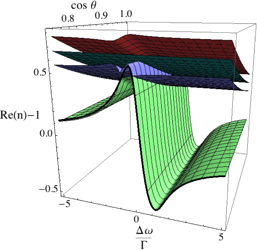
(a)  (b)

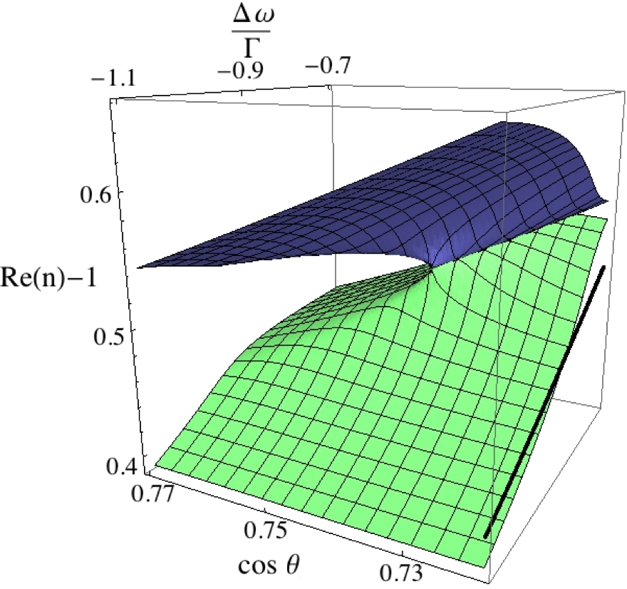
Figure 3: Four dispersion relations, corresponding to the real part of the refractive index, of radiation propagating through an atom-plasma mixture. $\text{Re}(n)-1$ is displayed as a function of the detuning $\Delta\omega=\omega-\omega_{0}$ of the radiation beam from atomic resonance, and of the angle $\theta$ between the radiation beam and the electron velocity. The black solid line displays the dispersion relation in absence of a plasma. Figure (b) shows a detail of figure (a).

Instead we discuss a specific numerical example. Experiments with cold beams of ammonia molecules can typically achieve densities of ${\cal N}_{\text{{\tiny A}}}=1.0\times 10^{9}\text{cm}^{-3}$ Motsch et al. (2009). Ammonia possesses an allowed electric-dipole transition at a resonance frequency of 23.7 GHz, with a transition dipole matrix element of $d_{eg}\approx 4.90\times 10^{-30}\text{Cm}$ Marquardt et al. (2003). We assume that the experimental environment induces an atomic decoherence rate of $\Gamma=20\,\text{s}^{-1}$ and work with a plasma electron density of ${\cal N}_{\text{e}}=1.5\times 10^{11}\text{cm}^{-3}$.

For the numerical values above, Fig. 3(a) shows the real part of the four poles, corresponding to four different dispersion relations. Far away from the region where the four poles are close to each other, they can be identified with specific physical phenomena. The green refractive index is then close to that of a pure atomic gas (solid black line in Fig. 3). The three poles that form parallel sheets correspond to an electrostatic wave that co-moves with the electrons at $n=\beta_{\|}^{-1}$, as well as two poles with refractive index $n=\beta_{\|}^{-1}(1\pm\frac{\omega_{\text{P}}}{\omega}\gamma^{-\frac{3}{2}})$, which are associated with the formation of volume plasmons.

The effect of the plasma becomes particularly pronounced in the area where all poles are close, which happens when the resonance condition $\beta_{\|}\approx n_{\text{{\tiny A}}}^{-1}$ is fulfilled. A detailed plot of this area is shown in in Fig. 3 b), which shows that the dispersion relations are strongly perturbed. In particular, the red dispersion relation in Fig. 4 shows a gain (negative imaginary part) for small negative detunings. This phenomenon has some relation to the formation of wave instabilities in Rydberg gases Shukla (2010), but in the current case it is resonantly enhanced. The energy for this process is provided by the kinetic energy of plasma electrons.

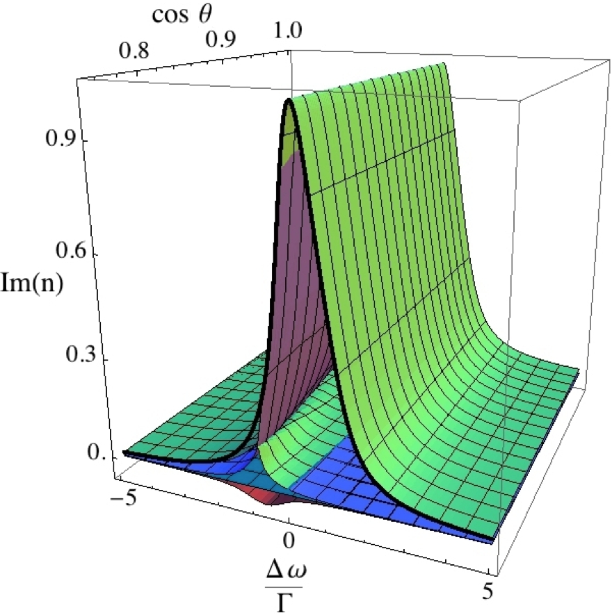
Figure 4: Absorption $\text{Im}(n)$ associated with the four dispersion relations. The solid black line represents absorption in a pure atomic gas.

Of equal interest is the behaviour of the amplitude factors ${\cal A}(s_{i})$, which multiply the partial radiation pulses in Eq. (18). At points, where the lower two dispersion relations of Fig. 3 meet, the amplitude of the partial pulse is enhanced. In particular, Fig. 5 shows that there are two points at which amplitude resonances occur. At these points, both real and imaginary part of the two dispersion relations are equal.

To understand the appearance of these resonances, we first consider an ideal, non-absorbing atom-plasma mixture with $\text{Im}(n_{\text{{\tiny A}}})=0$. For electrons moving at the speed $\beta_{\|}=n_{\text{{\tiny A}}}^{-1}$ the electrostatic dispersion relation $n=\beta_{\|}^{-1}$ matches the atomic dispersion relation $n=n_{\text{{\tiny A}}}$, so that both systems can be resonantly coupled. However, for real atoms, $n_{\text{{\tiny A}}}$ always possesses a non-vanishing imaginary part, see Eq. (13), so that a perfect match with the real dispersion relation $n=\beta_{\|}^{-1}$ would appear impossible. However, this argument neglects the influence of volume plasmons, which can modify the imaginary part of both dispersion relations. The strength of this effect depends on the ratio $r_{p}:=\omega_{\text{P}}/(\omega\sqrt{\gamma})$, see the discussion at the end of Sec. III. It is therefore possible for two complex dispersion relations to take the same values, if $r_{p}$ and $n_{\text{{\tiny A}}}$ (and thus $\Delta\omega$) take specific values.

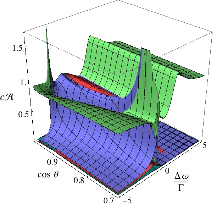
Figure 5: Field amplitude factors ${\cal A}(s_{i})$ of Eq. (18), in units of $c$, for the four dispersion relations. Sharp resonances occur at the points where two dispersion relations meet.

We have numerically evaluated under which conditions the two resonances do appear. For the numerical parameters given above, they only exist for $r_{p}$ between 0.05 and 0.2. Hence, the phenomenon occurs only within a narrow range of plasma electron densities. For $r_{p}\approx 0.05$, both resonances are close together and appear at high electron velocities $\beta_{\|}\approx 0.99$. As $r_{p}$ approaches the value 0.2, one resonance occurs at lower velocities, $\beta_{\|}\approx 0.75$, while the second resonance remains close to $\beta_{\|}\approx 0.99$. This is the case displayed in Fig. 5, where $r_{p}=0.12$.

V Pulse propagation

In Sec. IV we have identified specific values of radiation frequency $\omega$ and direction $\theta$ of the electrons for which the atom-plasma mixture acts like a resonant gain medium. In this section we simulate the propagation of a radiation pulse through such a medium.

We consider the situation that the pulse initially travels through a vacuum, which fills a region in space characterized by $z<0$, and enters the atom-plasma mixture (located in the region $z>0$) at a right angle. The pulse is much wider than its wavelength, so that its transverse profile does not change and the pulse is a function of $z$ and $t$ only. The polarization of the pulse is parallel to the atomic dipole moment $\bm{d}_{eg}$ so that the interaction with the atoms is maximized.

For mathematical reasons that are explained in App. C we assume that, while inside the vacuum, the pulse takes the form

$$E_{\text{free}}(t,z) =E_{\text{peak}}e^{-i\omega_{c}(t-t_{0})+ik_{c}z}\Pi\left(\frac{t-t_{0}-\frac{z}{c}}{T}\right)\frac{1}{2}\left[1+\cos\left(\frac{2\pi}{T}\left(t-t_{0}-\frac{z}{c}\right)\right)\right],$$ (20)

with $\Pi(x)$ is the boxcar function, which is 1 for $|x|<0.5$ and zero elsewhere. $E_{\text{free}}(t,z)$ describes a pulse that oscillates with central frequency $\omega_{c}$ and whose envelope is given by one period of the cosine function, so that it is similar to a Gaussian function but nonzero only in a time interval of width $T$. $k_{c}=\omega_{c}/c$ is the modulus of the central wavevector $\bm{k}_{c}$ that is shown in Fig. 1. The time $t_{0}$ can be chosen so that at $t=0$ the pulse is completely inside the vacuum.

The pulse enters the atom-plasma mixture at $z=0$, where the boundary conditions ensure continuity of $E(z,t)$. To find the evolution inside the mixture we need to integrate Eq. (17) numerically. We have seen in Sec. IV that if the electron velocity lies either in the plane spanned by $\hat{\bm{k}}$ and $\bm{e}_{{1}}$ or in the plane spanned by $\hat{\bm{k}}$ and $\bm{e}_{{2}}$, then the electric field can be reduced to a scalar equation, as in Eq. (19) for instance. We therefore only need to evaluate the 1D scalar form of Eq. (17) given by

$$E(z,t) =\int_{r-i\infty}^{r+i\infty}\frac{ds\,e^{ts}}{2\pi i}\int_{-\infty}^{\infty}\frac{dk}{(2\pi)^{\frac{1}{2}}}\,e^{ikz}E_{0}(k)\,R(k,s).$$ (21)

For the parameters used in Sec. IV, the numerical integration of Eq. (21) is not feasible because the integrand varies significantly on time scales $\Gamma^{-1}$, $\omega^{-1}$ and $\omega_{P}^{-1}$ that are many orders of magnitude apart. To avoid this problem, and for improved presentation, we have doubled the electron density, increased $\Gamma$ by a factor of $4\times 10^{8}$, and increased the atomic density by a factor of $3\times 10^{8}$, so that $\Gamma$ and $\omega_{P}$ are in the order of $0.1\,\omega$. We will comment on the differences for pulses under the more realistic conditions described in Sec. IV below.

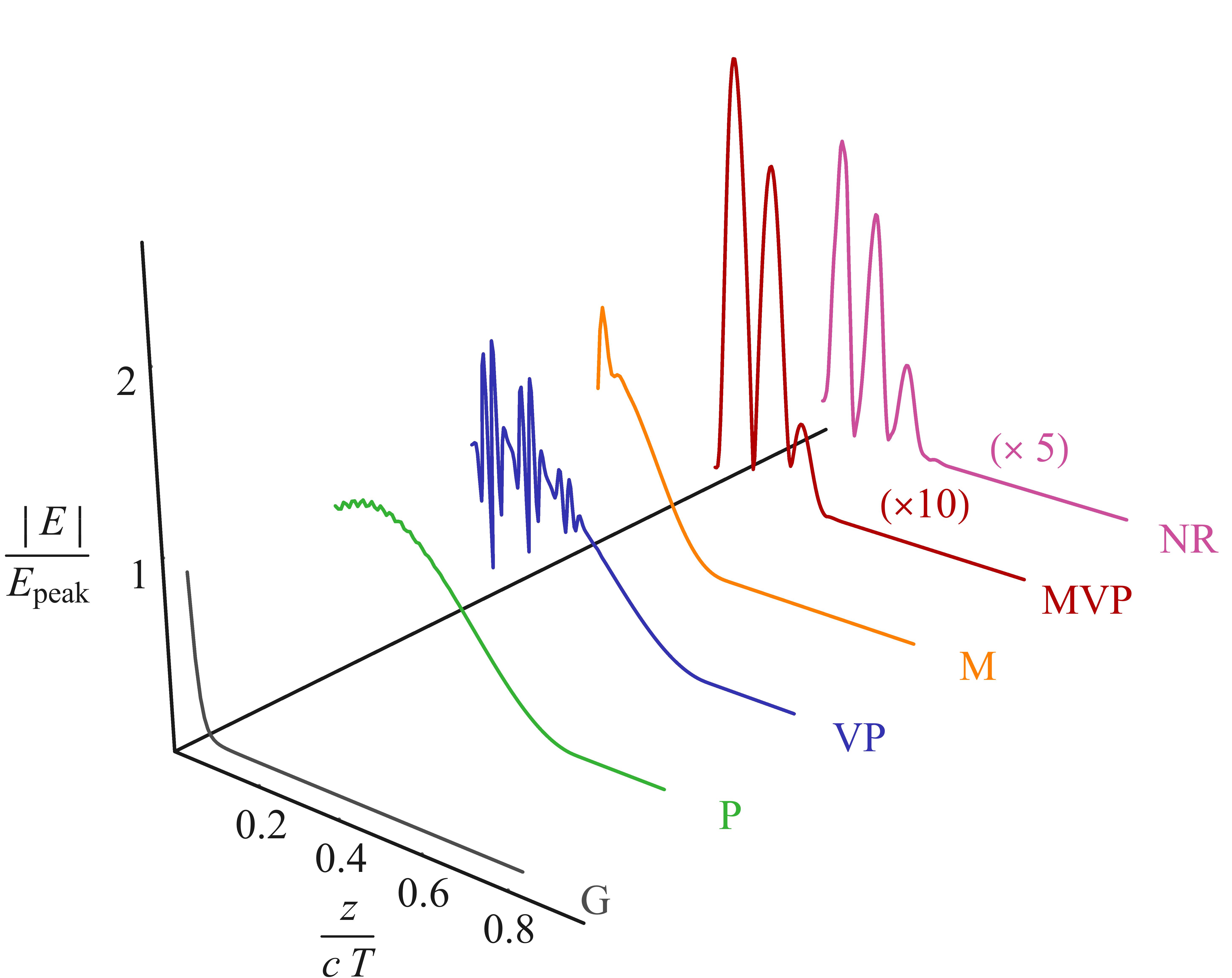
(a)           (b)

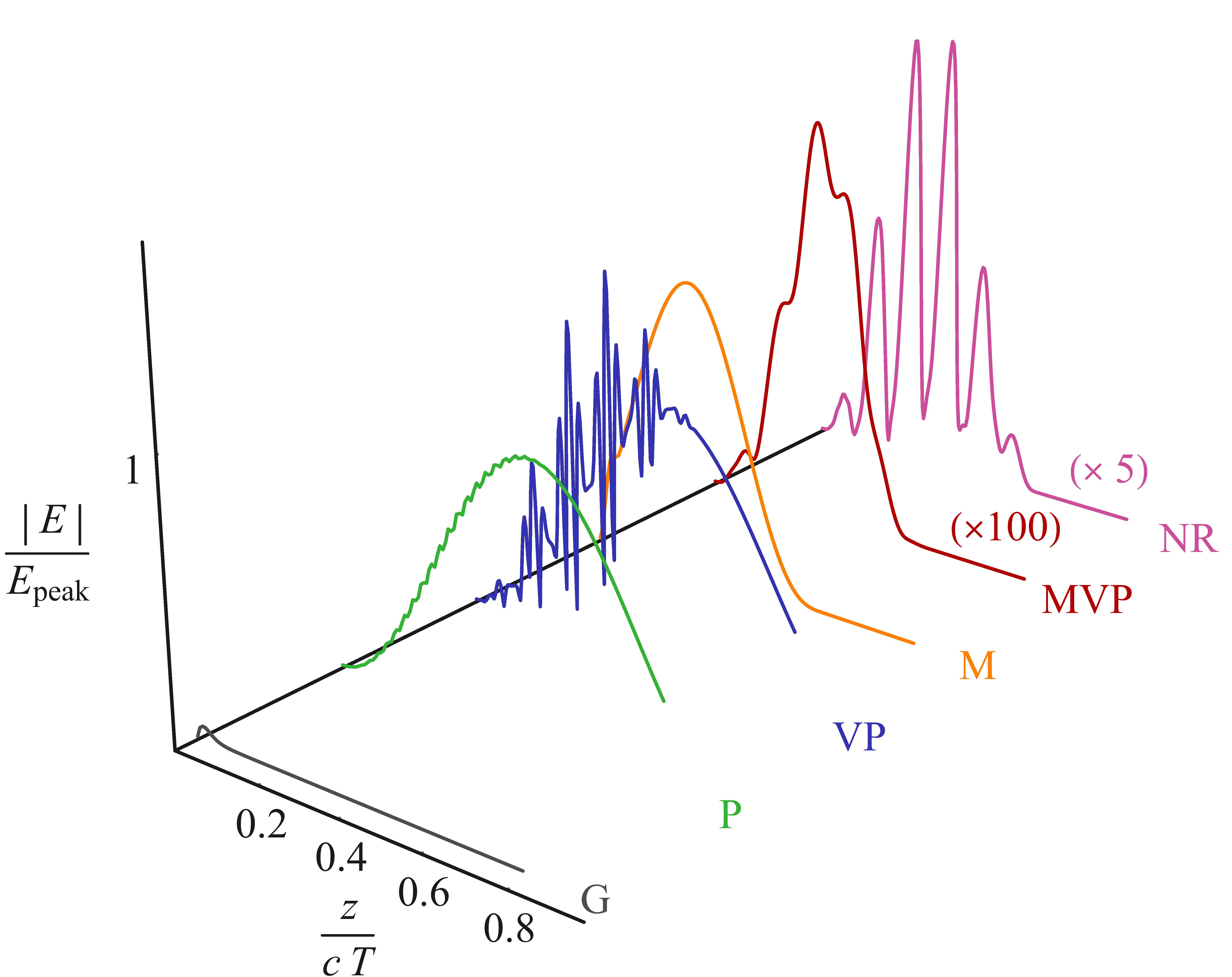
(c)

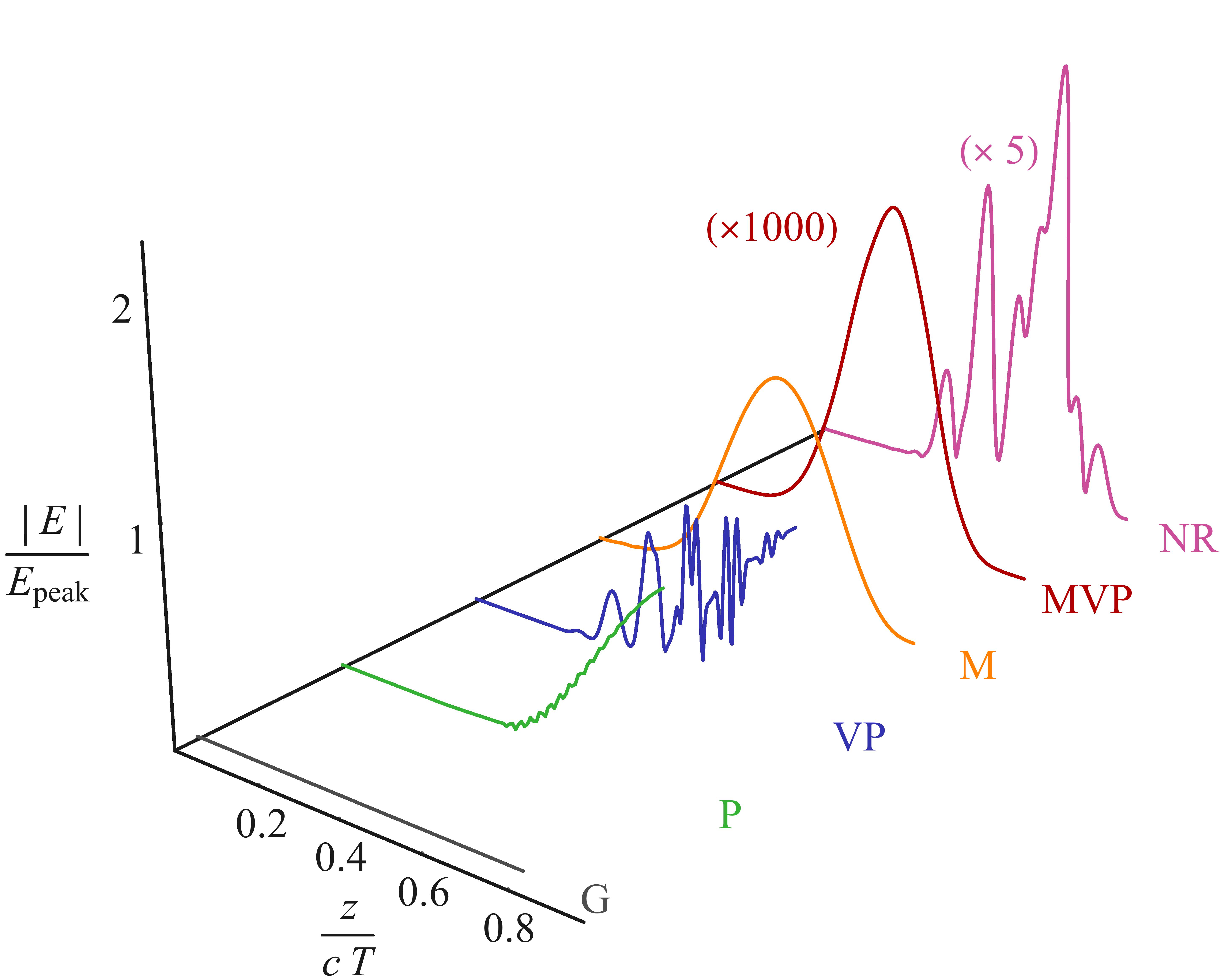
Figure 6: Propagation of light pulses through an atomic gas (G), a plasma (P), a plasma with volume plasmon generation (VP), an atom-plasma mixture (M), an atom-plasma mixture with volume plasmon generation (MVP), and a non-resonant atom-plasma mixture (NR). Shown is the electric field amplitude $|E(z,t)|$ in units of the peak amplitude $E_{\text{peak}}$ of the incoming pulse, as a function of position $z$ in units of the pulse width $cT$. Figures a-c correspond to three different instances in time.

Our numerical results for this choice of parameters are shown in Fig. 6, which displays the pulse for various media at three instances in time. Fig. 6(a) shows the pulse shortly after its peak entered the medium, and Figs. 6(b) and (c) show the same pulse at a time $0.4\,T$ and $0.8\,T$ later, where $T=20\,\Gamma^{-1}$ is the duration of the pulse.

The curve labelled “G” shows the pulse in an atomic gas in absence of a plasma. The gas is strongly absorbing, so that the pulse hardly enters the medium and is non-zero only for about $z<0.05\,cT$. In Fig. 6(c) the pulse is completely absorbed.

The curve labelled “P” shows the pulse inside a pure plasma where the electron velocity has no component along $\bm{e}_{{1}}$, so that no plasmons are generated. The pulse has essentially the same shape as in free space because $\omega_{\text{P}}$ is much smaller than $\omega$. The small ripples that can be seen on the tail of the pulse are an interference effect with a very small part of the pulse that corresponds to an electrostatic wave.

The curve labelled “VP” corresponds to a pure plasma with volume plasmon generation. As discussed in Sec. IV, the pulse is then decomposed into several components. The main part of the pulse propagates in a similar way as in absence of plasmons, but there are smaller pulse components that travel at different group velocities and produce an interference pattern. In Fig. 6(c) one can see that at this instance in time the slowest pulse components do not overlap with the main pulse anymore.

The curve labelled “M” displays an atom-plasma mixture without plasmon generation. The main part of the pulse travels at a group velocity that is comparable to that of the slow pulses in the VP case. The narrow peak in Fig. 6(a) corresponds to a pulse component that travels similarly to a pulse in an atomic gas and is quickly absorbed. The peak of the main pulse is increased, but only by about 10%.

The curve labelled “MVP” is the main result of this section and displays a pulse propagating through a mixture in the presence of plasmon generation. We have numerically determined that a resonance occurs for an electron direction of $\cos\theta\approx 0.714$ and a central pulse frequency of $\omega_{c}\approx 0.917\,\omega_{0}$. These are the values used for all five curves discussed so far. In Fig. 6(a) one can see that the pulse is split into different components and strongly enhanced. For presentational purposes we have rescaled the pulse: “$(\times 10)$” indicates that the field amplitude is actually 10 times larger than displayed. Fig. 6(b) demonstrates that the atom-plasma mixture acts as a gain medium for most of the pulse components. At the instant in time in Fig. 6(c), the pulse component with the largest gain factor dominates and is enhanced by a factor of about 2000. This demonstrates that atom-plasma mixtures may be able to amplify radiation.

To clearly distinguish the effect of the resonance we have also simulated a pulse labelled as “NR” that propagates in the same mixture but with a different central frequency $\omega_{c}=1.083\,\omega_{0}$, which corresponds to the same detuning from $\omega_{0}$ as in case MVP, but with opposite sign. Initially, the pulse has a similar shape as for the MVP case. Although it is smaller by a factor of about two, it still is enhanced compared to the free pulse by a factor of five. Fig. 6(b) shows that there is no further amplification of the pulse at this instance in time. In Fig. 6(c) one can see that one pulse component is enhanced. We attribute this late enhancement to the fact that the spectrum of the pulse is not confined to a specific frequency interval. Therefore, a small part of the pulse can still fulfill the resonance criteria and is enhanced in the same way as the red curve. However, the overall enhancement of the pulse lags behind the MVP case by a factor of about 200.

For the more realistic physical parameters used in Sec. IV, the pulse shape must be adapted to exhibit amplification. The most relevant change is the pulse duration, which must be in the order of $\Gamma^{-1}$ for resonant amplification and is therefore much longer than for the results presented in this section. However, the gain mechanism should work in a comparable way because the effect of the plasma on the refractive index is determined through the parameter $r_{p}=\omega_{\text{P}}/(\omega\sqrt{\gamma})$. This parameter is similar for the parameters used in Secs. IV and V.

One can estimate the gain for the parameters used in Sec. IV through the imaginary part of the refractive index displayed in Fig. 4. The negative value of Im$(n)\approx-0.05$ for the red dispersion relation generates an exponential gain factor $\exp(-\text{Im}(n)\omega z/c)$. This suggests that the radiation field would grow by a factor of 2 over a propagation length of 2.2 wavelengths, or 28 mm.

The results of this section demonstrate that volume plasmon generation is indeed the mechanism behind radiation amplification in atom-plasma mixtures. To achieve a high gain factor, the radiation pulse needs to have a frequency close to the volume plasmon resonance and a polarization that enables it to interact with the atoms. The plasma electrons must have an appropriate density, so that the plasma frequency is about 10-20% of the radiation frequency, and their velocity must be in a specific direction. If one of these conditions is not met, the mixture will not amplify the radiation pulse.

VI Conclusions

We have studied the properties of a near-resonant radiation pulse propagating through a mixture of two-level atoms and a classical, underdense, collision-less plasma. If the plasma electrons have a velocity component in the direction of the atomic dipole moment $\bm{d}_{eg}$, volume plasmons can be formed and optical dispersion relations are strongly modified, as shown in Fig. 3. For specific light frequencies $\omega$ and velocities of the electrons, resonances occur (see Fig. 6) and the mixture acts as a gain medium for radiation. This can happen if the plasma electrons travel at a speed comparable to the velocity of light in the atomic gas, and if the plasma frequency $\omega_{\text{P}}$ takes values between $0.05\,\omega$ and $0.2\,\omega$. We conclude from this analysis that radiation amplification through generation of volume plasmons should be possible if the assumptions described in section II are fulfilled.

However, more work is needed to understand whether light amplification via volume plasmons could also be used for non-classical states of light without destroying their coherence. Generating volume plasmons itself is a coherent process, but there are important secondary effects that have to be taken into account.

One such effect is the velocity distribution of plasma electrons, which may lead to inhomogenous broadening. For classical radiation, this effect is included in the general results derived above. However, a characterization of decoherence of a non-classical light pulse would require an extension of our methods. While decoherence due to inhomogeneous broadening could in principle be reversed Moiseev and Kröll (2001), the corresponding procedure would likely reduce the gain factor.

Furthermore, collisions of plasma electrons with other particles and ionization of atoms are irreversible processes that will decrease the coherence of a quantum state. These processes are not included in this study and may also modify the amplification of classical radiation pulses. Further studies are necessary to provide a quantitative estimate of this effect. In future work we will also investigate how the required speed of plasma electrons may be reduced through a superposition of light pulses.

Appendix A Equations of motion

A.1 Vlasov equation for relativistic plasmas

To describe plasma dynamics, we employ kinetic theory of a moving electron gas, in which the phase space density of electrons $f(\bm{r},\bm{p},t)$ evolves according to the relativistic Vlasov equation Liboff (2003)

$$\partial_{t}f+\frac{1}{m\gamma}\bm{p}\cdot\nabla_{\bm{r}}f+q\left[\bm{E}+\frac{1}{m\gamma}\bm{p}\times\bm{B}\right]\cdot\nabla_{\bm{p}}f=\left.\frac{df}{dt}\right|_{\text{cl.}}\!.$$ (22)

The right-hand side (r.h.s.) represents the contribution of collisions between the particles, which we ignore in this paper. Furthermore, we assume that the ions are not moving and that their spatial distribution ${\cal N}_{\text{I}}$ is homogeneous. Charge and current density of the plasma are then given by $\rho(\bm{r},t)=q{\cal N}_{\text{I}}-q\int d^{3}p\;f(\bm{r},\bm{p},t)$ and $\bm{J}(\bm{r},t)=-q\int d^{3}p\;\frac{\bm{p}}{m\gamma}\,f(\bm{r},\bm{p},t)$, respectively.

For weak electromagnetic fields, the Vlasov equation can be linearized in the deviation (1) of the electron distribution from the spatially homogeneous initial distribution $f_{0}(\bm{p})$. For quasi-neutral plasmas, where $\int d^{3}p\;f_{0}(\bm{p})={\cal N}_{\text{I}}$, we obtain Eq. (2) as dynamical equation. Charge and current density take the form

$$\rho(\bm{r},t) =-q\int d^{3}p\;\delta f(\bm{r},\bm{p},t),$$ (23)

$$\bm{J}(\bm{r},t) =-q\int d^{3}p\;\frac{1}{m\gamma}\bm{p}\,\delta f(\bm{r},\bm{p},t)\;.$$ (24)

Our main results are derived for general initial distributions $f_{0}(\bm{p})$, but our numerical examples consider plasma electrons with sharp momentum $\bm{p}_{\text{e}}=m\gamma\bm{v}_{\text{e}}$, so that

$$f_{0}(\bm{p})={\cal N}_{\text{e}}\delta(\bm{p}-\bm{p}_{\text{e}})\;,$$ (25)

with ${\cal N}_{\text{e}}$ the spatial electron density.

A.2 Equations of motion for the atomic gas

To describe the atomic gas we employ the method of coherence operators $\hat{\sigma}_{ij}(\bm{r})$ Fleischhauer and Lukin (2002), which are a set of operators that quantify superpositions between two atomic states $|i\rangle,|j\rangle$. If their mean value is zero, the atoms are in a state which does not include a superposition of these states. For $i=j$, coherence operators $\hat{\sigma}_{ii}(\bm{r})$ describe the population of the atomic state $|i\rangle$. Formally, coherence operators can be defined as

$$\hat{\sigma}_{ij}(\bm{r}) :=\frac{1}{{\cal N}_{\text{A}}}\int d^{3}r^{\prime}\,\hat{\Psi}_{i}(\bm{r}^{\prime})^{\dagger}\,\hat{\Psi}_{j}(\bm{r}^{\prime})\,S(\bm{r}-\bm{r}^{\prime})\,,$$ (26)

where $\hat{\Psi}_{i}(\bm{r})$ is an atomic field operator that annihilates an atom in internal state $|i\rangle$ at position $\bm{r}$ Zhang and Walls (1994); Lenz et al. (1994). $S(\bm{r}-\bm{r}^{\prime})$ is a smooth non-negative function that is zero if $\bm{r}^{\prime}\notin V_{S}(\bm{r})$, where $V_{S}(\bm{r})$ is an area of volume $V_{S}$ around $\bm{r}$. The function $S$ is approximately given by $S(\bm{r}-\bm{r}^{\prime})\approx V_{S}^{-1}$ for $\bm{r}^{\prime}\in V_{S}(\bm{r})$ and drops rapidly to zero around the boundary of $V_{S}(\bm{r})$, such that $\int d^{3}r\,S(\bm{r})=1$. In microscopic quantum electrodynamics one usually sets $S(\bm{r}-\bm{r}^{\prime})=\delta(\bm{r}-\bm{r}^{\prime})$. However, because we are employing macroscopic electrodynamics that is averaged over length scales large compared to atoms but small compared to the wavelength Jackson (1998), the same averaging has to be applied to all dynamical fields. This is accomplished through $S(\bm{r}-\bm{r}^{\prime})$ in Eq. (26). For a homogeneous atomic gas that initially is prepared in ground state $|g\rangle$, the atomic density is given by ${\cal N}_{\text{A}}=\langle\hat{\Psi}_{g}(\bm{r})^{\dagger}\,\hat{\Psi}_{g}(\bm{r})\rangle$.

The dynamics of coherence operators described by the Heisenberg equation of motion. In the presence of incoherent processes such as spontaneous emission, the Heisenberg-Langevin equation is used. Both require to evaluate the commutator, which is given by

$$[\hat{\sigma}_{ij}(\bm{r}),\hat{\sigma}_{kl}(\bm{r}^{\prime})] =\frac{\delta(\bm{r}-\bm{r}^{\prime})}{{\cal N}_{\text{A}}}\left\{\delta_{il}\sigma_{kj}(\bm{r})-\delta_{kj}\sigma_{il}(\bm{r})\right\}.$$ (27)

Strictly speaking, the $\delta$-distribution in this expression should be replaced by $S(\bm{r}-\bm{r}^{\prime})$. However, on the length scales of macroscopic electrodynamics, $S(\bm{r}-\bm{r}^{\prime})$ can be considered as a representation of the $\delta$-distribution.

Within the dipole approximation for atoms, coherence operators can provide a complete dynamical description, but because we are interested in the semi-classical properties of radiation propagation we restrict our considerations to the mean value $\sigma_{ij}(\bm{r})$ of the coherence fields and ignore field fluctuations. For two-level atoms, the equation relevant for the optical properties of the gas is then given by

$$\partial_{t}\sigma_{eg}(\bm{r},t) =\left(-i\omega_{0}-\frac{\Gamma}{2}\right)\sigma_{eg}(\bm{r},t)+\frac{i}{\hbar\varepsilon_{0}}\bm{D}_{\perp}(\bm{r})\cdot\bm{d}_{eg}^{\,*}(\sigma_{gg}(\bm{r})-\sigma_{ee}(\bm{r}))\;,$$ (28)

with $\Gamma$ the atomic spectral line width, $\bm{d}_{eg}$ the electric-dipole moment of the atoms, and $\bm{D}$ the electric displacement field. The notation $(\cdots)_{\perp}$ indicates that only the transverse part of a vector field is considered. In Fourier space, the transverse part of an arbitrary vector field $\bm{V}(\bm{k})$ can be found using

$$V_{\perp,i}(\bm{k})=\left(\delta_{ij}-\hat{\bm{k}}_{i}\hat{k_{j}}\right)V_{j}(\bm{k})\;,$$ (29)

with $\hat{\bm{k}}$ of Eq. (9).

For small radiation intensities we can make the low-saturation approximation by setting $\sigma_{gg}(\bm{r})\approx 1$ and $\sigma_{ee}(\bm{r})\approx 0$. In rotating-wave approximation Cohen-Tannoudji et al. (2008), the atomic dynamics is then described by Eq. (4).

A.3 Coupled equations of motion

The atomic dynamical equation (4) and the Vlasov equation (2) are coupled through an electromagnetic field, which evolves according to the macroscopic Maxwell equations. In the associated material equation $\bm{D}=\varepsilon_{0}\bm{E}+\bm{P}$, the polarization field contains the contribution of bound charges, i.e., the atoms and molecules, and is given by the transverse part of Eq. (3). The longitudinal part can be neglected because it is only off-resonantly coupled to the radiation. A spatial Fourier transform $\bm{r}\rightarrow\bm{k}$, and a temporal Laplace transform $t\rightarrow s$ of all dynamical equations yields

$$\delta f(\bm{k},\bm{p},s) =\frac{1}{s+i\frac{\bm{k}\cdot\bm{p}}{m\gamma}}\bigg{[}\delta f(\bm{k},\bm{p},t=0)+q\Big{(}\bm{E}(\bm{k},s)+\frac{1}{m\gamma}\bm{p}\times\bm{B}(\bm{k},s)\Big{)}\cdot\nabla_{\bm{p}}f_{0}(\bm{p})\bigg{]},$$ (30)

$$\sigma_{eg}(\bm{k},s) =\frac{\sigma_{eg}(\bm{k},t=0)+\frac{i}{\hbar\varepsilon_{0}}\bm{D}_{\perp}(\bm{k},s)\cdot\bm{d}_{eg}^{\,*}}{s+i\omega_{0}+\frac{\Gamma}{2}},$$ (31)

$$i\bm{k}\cdot\bm{D}(\bm{k},s) =\rho(\bm{k},s),$$ (32)

$$i\bm{k}\cdot\bm{B}(\bm{k},s) =0,$$ (33)

$$i\bm{k}\times\bm{E}(\bm{k},s) =-s\bm{B}(\bm{k},s)+\bm{B}(\bm{k},t=0),$$ (34)

$$i\bm{k}\times\bm{B}(\bm{k},s) =\mu_{0}\left(\bm{J}(\bm{k},s)+s\bm{D}(\bm{k},s)-\bm{D}(\bm{k},t=0)\right).$$ (35)

In rotating-wave approximation, the material equations take the explicit form

$$\bm{D}_{\perp}(\bm{k},t) =\varepsilon_{0}\bm{E}_{\perp}(\bm{k},t)+{\cal N}_{\text{{\tiny A}}}\,\bm{d}_{\perp}(\hat{\bm{k}})\sigma_{eg}(\bm{k}),$$ (36)

$$D_{\|}(\bm{k},t) =\varepsilon_{0}E_{\|i}(\bm{k},t),$$ (37)

with $\bm{d}_{\perp}(\hat{\bm{k}})$ of Eq. (10).

Appendix B Solving the equations of motion

We assume that atoms are initially in their ground state, $\sigma_{eg}(t=0)=0$, and that the initial state of the plasma electrons is given by $f_{0}$, so that $\delta f(\bm{k},\bm{p},t=0)=0$. The incoming electromagnetic field (radiation pulse) is characterized by the initial amplitudes $\bm{B}_{0}(\bm{k}):=\bm{B}(\bm{k},t=0)$ and $\bm{D}_{0}(\bm{k}):=\bm{D}(\bm{k},t=0)$.

Using Eq. (36), the electromagnetic field can be expressed in terms of $\sigma_{eg}$ and $\delta f$ as

$$\bm{B}(\bm{k},s) =\frac{1}{s}\left(\bm{B}_{0}(\bm{k})-i\bm{k}\times\bm{E}_{\perp}(\bm{k},s)\right),$$ (38)

$$E_{\parallel}(\bm{k},s) =-\frac{i}{k\varepsilon_{0}}\rho(\bm{k},s),$$ (39)

$$\bm{E}_{\perp}(\bm{k},s) =\frac{1}{c^{2}k^{2}+s^{2}}\Big{(}\frac{s}{\varepsilon_{0}}\left(\bm{D}_{0}(\bm{k})-\bm{J}_{\perp}(\bm{k},s)\right)+ic^{2}\bm{k}\times\bm{B}_{0}(\bm{k})-\frac{s^{2}{\cal N}_{\text{{\tiny A}}}}{\varepsilon_{0}}\bm{d}_{\perp}\big{(}\hat{\bm{k}}\big{)}\,\sigma_{eg}(\bm{k},s)\Big{)},$$ (40)

$$\bm{D}_{\perp}(\bm{k},s) =\frac{1}{c^{2}k^{2}+s^{2}}\Big{(}s\left(\bm{D}_{0}(\bm{k})-\bm{J}_{\perp}(\bm{k},s)\right)+\frac{i}{\mu_{0}}\bm{k}\times\bm{B}_{0}(\bm{k})+k^{2}c^{2}{\cal N}_{\text{{\tiny A}}}\bm{d}_{\perp}\big{(}\hat{\bm{k}}\big{)}\,\sigma_{eg}(\bm{k},s)\Big{)}\;.$$ (41)

Inserting Eq. (41) into Eq. (31) we obtain

$$\sigma_{eg}(\bm{k},s) =\frac{\left(is\left(\bm{D}_{0}(\bm{k})-\bm{J}_{\perp}(\bm{k},s)\right)-\frac{\bm{k}\times\bm{B}_{0}(\bm{k})}{\mu_{0}}\right)\cdot\bm{d}_{eg}^{\,*}}{\hbar\varepsilon_{0}\Delta(\bm{k},s)},$$ (42)

$$\Delta(\bm{k},s) :=(c^{2}k^{2}+s^{2})\left(s+i\omega_{0}+\frac{\Gamma}{2}\right)-ik^{2}c^{2}\eta\big{(}\hat{\bm{k}}\big{)},$$ (43)

with $\eta\big{(}\hat{\bm{k}}\big{)}$ of Eq. (14). Inserting the atomic polarization (42) into Eq. (40) yields

$$\bm{E}_{\perp}(\bm{k},s) =\frac{1}{\varepsilon_{0}}\frac{\left(\bm{X}(\bm{k},s)-s\bm{J}_{\perp}(\bm{k},s)\right)\cdot\stackrel{{\scriptstyle\leftrightarrow}}{{{\cal E}^{(\text{A})}}}(\bm{k},s)}{c^{2}k^{2}+s^{2}},$$ (44)

$$\bm{X}(\bm{k},s) :=\frac{i}{\mu_{0}}\bm{k}\times\bm{B}_{0}(\bm{k})+s\bm{D}_{0}(\bm{k}),$$ (45)

$${\cal E}^{(\text{A})}_{ij}(\bm{k},s) :=\delta_{ij}-i\frac{s^{2}}{\Delta(\bm{k},s)}\frac{{\cal N}_{\text{{\tiny A}}}}{\hbar\varepsilon_{0}}\bm{d}_{eg,i}^{\,*}\bm{d}_{\perp,j}\big{(}\hat{\bm{k}}\big{)}\;.$$ (46)

The tensor ${\cal E}^{(\text{A})}$ describes the polarization-dependent response of the atomic medium to the radiation field. $\bm{X}$ depends only on the initial radiation field. Inserting Eq. (44) into (30) yields

$$\delta f(\bm{k},\bm{p},s) =\frac{q}{\varepsilon_{0}}\Bigg{\{}\frac{\left(\bm{X}(\bm{k},s)-s\bm{J}_{\perp}(\bm{k},s)\right)\cdot\stackrel{{\scriptstyle\leftrightarrow}}{{{\cal E}^{(\text{A})}}}(\bm{k},s)}{c^{2}k^{2}+s^{2}}+\frac{\bm{p}\times\left(\bm{k}\times\left(\bm{X}-s\bm{J}_{\perp}\right)\cdot\stackrel{{\scriptstyle\leftrightarrow}}{{{\cal E}^{(\text{A})}}}(\bm{k},s)\right)}{ism\gamma(c^{2}k^{2}+s^{2})}$$

$$\hskip 11.38109pt+\frac{\rho(\bm{k},s)}{ik^{2}}\bm{k}+\varepsilon_{0}\frac{\bm{p}\times\bm{B}_{0}(\bm{k})}{sm\gamma}\Bigg{\}}\cdot\frac{\nabla_{\bm{p}}f_{0}(\bm{p})}{s+i\frac{\bm{k}\cdot\bm{p}}{m\gamma}}.$$ (47)

Eq. (47) could be used to derive charge and current density distribution. However, it is physically more instructive to use Eq. (30) instead. Multiplying it with $-q$ and integrating over $d^{3}p$ gives a relation between charge distribution and radiation field,

$$\rho(\bm{k},s) =-q^{2}\bm{E}(\bm{k},s)\cdot\int d^{3}p\,\frac{\nabla_{\bm{p}}f_{0}(\bm{p})}{s+i\bm{k}\cdot\bm{p}/(m\gamma)}-q^{2}\bm{B}(\bm{k},s)\cdot\int\frac{d^{3}p}{m\gamma s+i\bm{k}\cdot\bm{p}}\nabla_{\bm{p}}f_{0}(\bm{p})\times\bm{p}\;.$$ (48)

Exploiting $\nabla_{\bm{p}}m\gamma=\bm{p}/(m\gamma c^{2})$ and performing a partial integration gives

$$\rho(\bm{k},s) =\varepsilon_{0}\bm{E}(\bm{k},s)\cdot\left(i\bm{k}\partial_{s}{\cal Z}(\bm{k},s)-\frac{1}{c^{2}}(\bm{k}\cdot\nabla_{\bm{k}})\bm{{\cal Z}}(\bm{k},s)\right)+\varepsilon_{0}\bm{B}(\bm{k},s)\cdot\left(\bm{k}\times\nabla_{\bm{k}}{\cal Z}(\bm{k},s)\right)\;,$$ (49)

where we have introduced the notation

$${\cal Z}(\bm{k},s) :=\frac{q^{2}}{\varepsilon_{0}}\int\frac{d^{3}p}{m\gamma}\;\frac{f_{0}(\bm{p})}{s+i\bm{k}\cdot\bm{p}/(m\gamma)},$$ (50)

$$\bm{{\cal Z}}(\bm{k},s) :=\frac{q^{2}}{\varepsilon_{0}}\int\frac{d^{3}p}{(m\gamma)^{2}}\;\frac{f_{0}(\bm{p})}{s+i\bm{k}\cdot\bm{p}/(m\gamma)}\bm{p},$$ (51)

$$\Omega_{\text{P}}^{2} :=\frac{q^{2}}{\varepsilon_{0}}\int\frac{d^{3}p}{m\gamma}\;f_{0}(\bm{p})\;.$$ (52)

${\cal Z}$ is a relativistic generalization of the plasma dispersion function, which takes the same form with $\gamma=1$ Sitenko and Malnev (1995). $\bm{{\cal Z}}$ is related to the dispersion function through $i\partial_{s}\bm{{\cal Z}}=\nabla_{\bm{k}}{\cal Z}$. The relativistic plasma frequency $\Omega_{\text{P}}$, which coincides with the standard plasma frequency $\omega_{\text{P}}$ in the limit $\gamma\rightarrow 1$, fulfills $i\bm{k}\cdot\bm{{\cal Z}}=\Omega_{\text{P}}^{2}-s{\cal Z}$.

Relation $\bm{E}(\bm{k},s)\cdot\bm{k}=kE_{\parallel}=-i\rho/\varepsilon_{0}$ enables us to express the charge density as

$$\rho(\bm{k},s)=\frac{\zeta\varepsilon_{0}}{1-\partial_{s}{\cal Z}}\Bigg{(}\frac{1}{c^{2}}\bm{E}(\bm{k},s)\cdot\left(\bm{{\cal Z}}+s\partial_{s}\bm{{\cal Z}}\right)-i\left(\bm{k}\times\bm{B}(\bm{k},s)\right)\cdot\partial_{s}\bm{{\cal Z}}\Bigg{)}\;.$$ (53)

In this result, we introduced a parameter $\zeta$, which enables us to evaluate the non-relativistic limit. $\zeta=1$ corresponds to the full relativistic treatment, while $\zeta=0$ neglects the coupling to the magnetic field and relativistic corrections.

The current density (24) can be found in a similar way. Using Eq. (30) again we find

$$\bm{J}(\bm{k},s) =\varepsilon_{0}\bm{E}(\bm{k},s){\cal Z}+\rho(\bm{k},s)\partial_{s}\bm{{\cal Z}}-\zeta\varepsilon_{0}\bm{B}(\bm{k},s)\times\bm{{\cal Z}}+i\zeta\varepsilon_{0}\left[\left(i\bm{k}\times\bm{B}(\bm{k},s)-\frac{s}{c^{2}}\bm{E}(\bm{k},s)\right)\cdot\nabla_{\bm{k}}\right]\bm{{\cal Z}}.$$ (54)

Solving the system of equations (53), (54), (44), and (38) is a straightforward but tedious task. The first step is to express charge and current density in terms of transverse electromagnetic fields,

$$\rho(\bm{k},s) =\zeta\frac{\varepsilon_{0}}{s}\left(\rho_{0}(\bm{k},s)+\bm{\rho}_{1}(\bm{k},s)\cdot\bm{E}_{\perp}(\bm{k},s)\right),$$ (55)

$$\bm{J}_{\perp}(\bm{k},s) =\frac{\varepsilon_{0}}{s}\left(\zeta\bm{J}_{0}(\bm{k},s)+\bm{E}_{\perp}(\bm{k},s)\cdot\stackrel{{\scriptstyle\leftrightarrow}}{{{\cal M}}}\right),$$ (56)

$$\rho_{0}(\bm{k},s) :=\frac{-i}{({\cal Z}_{\perp}+1)}(\bm{k}\times\bm{B}_{0})\cdot\partial_{s}\bm{{\cal Z}},$$ (57)

$$\bm{\rho}_{1}(\bm{k},s) :=\frac{1}{c^{2}({\cal Z}_{\perp}+1)}\bm{U},$$ (58)

$$(\bm{J}_{0}(\bm{k},s))_{n} :=-(\bm{k}\times\bm{B}_{0})_{i}\Big{[}i\frac{\bm{U}_{n}\,\partial_{s}\bm{{\cal Z}}_{\perp,i}}{c^{2}k^{2}({\cal Z}_{\perp}+1)}+\left(\frac{\partial\bm{{\cal Z}}_{n}}{\partial k_{i}}\right)_{\perp}\Big{]}+\frac{i(s{\cal Z}-\Omega_{\text{p}}^{2})}{k^{2}}(\bm{k}\times\bm{B}_{0})_{n},$$ (59)

with

$${\cal M}_{in} :=\zeta\frac{U_{i}U_{n}}{k^{2}c^{4}({\cal Z}_{\perp}+1)}-i\zeta\frac{k^{2}c^{2}+s^{2}}{c^{2}}\left(\frac{\partial\bm{{\cal Z}}_{n}}{\partial k_{i}}\right)_{\perp}+\left(\zeta\Omega_{\text{P}}^{2}+(1-\zeta)s{\cal Z}\right)\left(\delta_{in}\right)_{\perp},$$ (60)

$$\bm{U} :=(k^{2}c^{2}+s^{2})\partial_{s}\bm{{\cal Z}}_{\perp}+s\bm{{\cal Z}}_{\perp},$$ (61)

$${\cal Z}_{\perp} :=\frac{1}{k^{2}c^{2}}\left(\Omega_{\text{P}}^{2}-(k^{2}c^{2}+s^{2})\partial_{s}{\cal Z}-2s{\cal Z}\right).$$ (62)

These quantities describe the dependence of the optical properties on the plasma electron density, temperature, and mean velocity. The notation $(\cdots)_{\perp}$ implies again that all indices have been transversalized according to Eq. (29). The final result for the electric field then takes the form (11), with

$$\stackrel{{\scriptstyle\leftrightarrow}}{{R}}(\bm{k},s) =-\stackrel{{\scriptstyle\leftrightarrow}}{{{\cal M}}}_{0}\cdot\left((k^{2}c^{2}+s^{2})\stackrel{{\scriptstyle\leftrightarrow}}{{{\cal E}^{(\text{A})}}}^{-1}+\stackrel{{\scriptstyle\leftrightarrow}}{{{\cal M}}}\right)^{-1},$$ (63)

$$\left(\stackrel{{\scriptstyle\leftrightarrow}}{{{\cal M}}}_{0}\right)_{in} :=\frac{i\zeta}{kc^{3}(1+{\cal Z}_{\perp})}\partial_{s}\bm{{\cal Z}}_{\perp,i}U_{n}+\zeta\frac{k}{c}\left(\frac{\partial\bm{{\cal Z}}_{n}}{\partial k_{i}}\right)_{\perp}+\frac{i}{ck}\left(ck(ck+is)-\zeta s{\cal Z}+\zeta\Omega_{\text{P}}^{2}\right)\left(\delta_{in}\right)_{\perp}.$$ (64)

In this expression, we have assumed that the initial field amplitudes $\bm{B}_{0}(\bm{k})$ and $\bm{E}_{0}(\bm{k})$ are transverse vector fields, are are related as in free space through $\bm{k}\times\bm{B}_{0}(\bm{k})=-\bm{E}_{0}(\bm{k})\,k/c$.

B.1 Pure atomic gas

Expression (63) can be cast into a physically more intuitive form if one relates $\stackrel{{\scriptstyle\leftrightarrow}}{{{\cal E}^{(\text{A})}}}$ to the atomic refractive index $n_{\text{{\tiny A}}}$. To do this, we temporarily assume that the plasma density vanishes, so that

$$\bm{E}(\bm{k},s) =-i\frac{ck+is}{k^{2}c^{2}+s^{2}}\bm{E}_{0}(\bm{k})\cdot\stackrel{{\scriptstyle\leftrightarrow}}{{{\cal E}^{(\text{A})}}}\;.$$ (65)

Here, and in the more general expression (63), all vectors that multiply $\stackrel{{\scriptstyle\leftrightarrow}}{{{\cal E}^{(\text{A})}}}$ from the left are transverse. We therefore can replace $\stackrel{{\scriptstyle\leftrightarrow}}{{{\cal E}^{(\text{A})}}}$ by its transverse part ${\cal E}^{(\text{A})\perp}$, which is found using Eq. (29). This matrix has three left-eigenvectors, which are given by $\hat{\bm{k}}$, $\bm{e}_{{1}}$ and $\bm{e}_{{2}}$ of Eq. (9). The eigenvalue of $\hat{\bm{k}}$ is zero because ${\cal E}^{(\text{A})\perp}$ is a transverse tensor, and the eigenvalue of $\bm{e}_{{2}}\big{(}\hat{\bm{k}}\big{)}$ is unity, because the atoms are transparent for radiation with this polarization. For radiation with polarization $\bm{e}_{{1}}\big{(}\hat{\bm{k}}\big{)}$, the interaction with the atoms is described through the relation

$$\bm{e}_{{1}}\cdot{\cal E}^{(\text{A})\perp}(\bm{k},s) =\left(1-i\frac{s^{2}\eta\big{(}\hat{\bm{k}}\big{)}}{\Delta(\bm{k},s)}\right)\bm{e}_{{1}}.$$ (66)

For radiation with initial amplitude $\bm{E}_{0}(\bm{k})=E_{0}(\bm{k})\,\bm{e}_{{1}}$, the evolution equation becomes

$$E(\bm{k},s) =\frac{(s-ick)\left(\Gamma-2i\eta+2s+2i\omega_{0}\right)}{2i\omega_{0}\left(c^{2}k^{2}+s^{2}\right)+c^{2}k^{2}(\Gamma-2i\eta+2s)+s^{2}(\Gamma+2s)}E_{0}(\bm{k}).$$ (67)

The roots of the denominator determine the dispersion relation. Setting $s=-i\omega$ and $k=n_{\text{{\tiny A}}}(\omega)\omega/c$, and solving for the atomic refractive index we find $n_{\text{{\tiny A}}}$ of Eq. (13).

Conversely, we can express $\eta\big{(}\hat{\bm{k}}\big{)}$ of Eq. (14) through the refractive index,

$$\eta\big{(}\hat{\bm{k}}\big{)} =\left(1-\frac{1}{n_{\text{{\tiny A}}}^{2}\big{(}\omega,\hat{\bm{k}}\big{)}}\right)\left(-i\frac{\Gamma}{2}-(\omega-\omega_{0})\right).$$ (68)

If we reinsert this expression into Eq. (46) we get

$${\cal E}^{(\text{A})\perp}(\bm{k},s) =\bm{e}_{{1}}^{\,*}\otimes\bm{e}_{{1}}\frac{\omega^{2}-k^{2}c^{2}}{n_{\text{{\tiny A}}}^{2}(\omega,\hat{k})\,\omega^{2}-k^{2}c^{2}}+\bm{e}_{{2}}^{\,*}\otimes\bm{e}_{{2}}.$$ (69)

Returning to the propagator (63) in the presence of a plasma, the dynamics of the electric field amplitude takes the form (12)

Appendix C Propagation of radiation pulses

Our task is to evaluate the pulse amplitude for $t>0$ inside the atom-plasma mixture ($z>0$). Under these circumstances, the factor $e^{ikz}$ in Eq. (21) guarantees that the integrand decreases to zero for $|k|\rightarrow\infty$ and Im$(k)>0$ as long as the factor $E_{0}(k)\,R(k,s)$ does not increase indefinitely. In this case we can close the $k$-integral in the upper half-plane and use the Residue theorem for its evaluation.

Due to the fact that $R(k,s)$ is a known rational function, the requirement that $E_{0}(k)\,R(k,s)$ remains finite poses a condition on the shape of the initial pulse $E_{0}(z)$, which for instance excludes a Gaussian shape of the initial pulse. We have verified that our method can indeed not be applied to Gaussian pulses and therefore have chosen an initial pulse of the form (20).

We can then use the Residue theorem to evaluate the $k$-integration. denoting by $k_{l}(s),l=1,2,\cdots,L$ the poles of the integrand in the upper half of the complex $k$-plane, the field can be expressed as

$$E(z,t) =\frac{1}{\sqrt{2\pi}}\int_{r-i\infty}^{r+i\infty}ds\,e^{ts}\sum_{l}e^{ik_{l}(s)z}E_{0}(k_{l}(s))R_{l}(s),$$ (70)

where $R_{l}(s)=\text{Res}\left(R(k,s),k\rightarrow k_{l}(s)\right)$ denotes the residue of $R(k,s)$ at the $l$th pole.

The integral over $s=r-i\omega$ can be evaluated numerically, but one has to choose the parameter $r$ carefully. To understand this, consider a simple example of a medium with some given refractive index $n^{2}(s)=1+\chi(s)$, where $\chi(s)$ is the Laplace transform of the linear susceptibility $\chi(t)$. For such a medium, the denominator of $R(k,s)$ takes the form $k^{2}c^{2}+s^{2}n^{2}(s)$, so that the poles are at $k_{l}(s)=\pm isn(s)/c$. If we consider the usual situation where Re$(n)>0$, then only the pole $k_{l}(s)=isn(s)/c$ propagates to the right. Let us assume for now that $s=-i\omega$ for real frequencies $\omega$. For an absorbing medium we have Im$(n)>0$ so that the pole lies in the upper half and one recovers the usual result for a pulse propagating through an absorbing medium. However, for a gain medium the pole would be in the lower half and therefore would not contribute to Eq. (70). We remark that this problem is not resolved by the Kramers-Kronig relations. The latter imply that all poles of $n(s)$ are in the lower half plane, but this does not restrict the location of the poles $\pm isn(s)/c$ in complex $k$-plane.

This problem can be resolved by recalling that $s=r-i\omega$ has a positive real part $r$ that has to be larger than the real part of all poles in the $s$-plane. However, increasing $r$ also affects the pole $k_{l}(s)=isn(s)/c$ in the $k$-plane and increases its imaginary part. For large enough $r$ one can achieve that the imaginary parts of all poles $k_{l}(s)$ (for which the real part is positive so that they propagate to the right) are positive and thus contribute to Eq. (70). In our numerical evaluations, we have used a value of $r=0.0173\,\omega_{0}$ for all pulses displayed in Fig. 6.

The last step is to implement the proper initial conditions for $E(z,t)$. For the situation considered in this section, the boundary conditions at the interface between mixture and vacuum are that $E(z,t)$ and its derivatives with respect to $z$ are continuous at $z=0$. Eq. (70) implies that the temporal Laplace transform of $E(z,t)$ is given by

$$E(z,s) =\sqrt{2\pi}i\sum_{l}e^{ik_{l}(s)z}E_{0}(k_{l}(s))R_{l}(s).$$ (71)

We can then form a set of $L$ coupled linear equations

$$\left.\partial_{z}^{l}E(z,s)\right|_{z=0} =\left.\partial_{z}^{l}E_{\text{free}}(z,s)\right|_{z=0}\quad,\;l=1,2,\cdots,L$$ (72)

and solve this for the unknown parameters $E_{0}(k_{l}(s))$, thus expressing the relevant initial conditions $E_{0}(k_{l}(s))$ through the incoming pulse $E_{\text{free}}(z,t)$. It then only remains to numerically integrate the resulting integral over $s$, which can be done with standard algorithms provided by Mathematica.

References

- Chang et al. (2007) D. E. Chang, A. S. Sørensen, E. A. Demler, and M. D. Lukin, Nature Physics 3, 807 (2007).
- Nie and Emory (1997) S. Nie and S. R. Emory, Science 275, 1102 (1997).
- Schmidt and Imamoǧlu (1996) H. Schmidt and A. Imamoǧlu, Opt. Lett. 21, 1936 (1996).
- Hau et al. (1999) L. V. Hau, S. E. Harris, Z. Dutton, and C. H. Behroozi, Nature 397, 594 (1999).
- Kang and Zhu (2003) H. Kang and Y. Zhu, Phys. Rev. Lett. 91, 093601 (2003).
- Wang et al. (2006) Z.-B. Wang, K.-P. Marzlin, and B. C. Sanders, Phys. Rev. Lett. 97, 063901 (2006).
- Guerreiro et al. (2014) T. Guerreiro, A. Martin, B. Sanguinetti, J. S. Pelc, C. Langrock, M. M. Fejer, N. Gisin, H. Zbinden, N. Sangouard, and R. T. Thew, Phys. Rev. Lett. 113, 173601 (2014).
- Kulin et al. (2000) S. Kulin, T. C. Killian, S. D. Bergeson, and S. L. Rolston, Phys. Rev. Lett. 85, 318 (2000).
- Fletcher et al. (2006) R. S. Fletcher, X. L. Zhang, and S. L. Rolston, Phys. Rev. Lett. 96, 105003 (2006).
- Simien et al. (2004) C. E. Simien, Y. C. Chen, P. Gupta, S. Laha, Y. N. Martinez, P. G. Mickelson, S. B. Nagel, and T. C. Killian, Phys. Rev. Lett. 92, 143001 (2004).
- Killian et al. (2005) T. C. Killian, Y. C. Chen, P. Gupta, S. Laha, Y. N. Martinez, P. G. Mickelson, S. B. Nagel, A. D. Saenz, and C. E. Simien, J. Phys. B 38, S351 (2005).
- Mendonça et al. (2009) J. T. Mendonça, J.Loureiro, and H. Terças, J. Plasma Phys. 75, 713 (2009).
- Shukla (2010) P. Shukla, Phys. Lett. A 374, 3656–3657 (2010).
- Lu et al. (2011) R. Lu, L. Guo, J. Guo, and S. Han, Phys. Lett. A 375, 2158ミ2161 (2011).
- Mendonça et al. (2010) J. T. Mendonça, N. Shukla, and P. K. Shukla, J. Plasma Phys. 76, 19 (2010).
- Baranger and Mozer (1961) M. Baranger and B. Mozer, Phys. Rev. 123, 25 (1961).
- Kunze and Griem (1968) H. J. Kunze and H. R. Griem, Phys. Rev. Lett. 21, 1048 (1968).
- Cooper and Ringler (1969) W. S. Cooper and H. Ringler, Phys. Rev. 179, 226 (1969).
- Sprangle et al. (1990a) P. Sprangle, E. Esarey, and A. Ting, Phys. Rev. Lett. 64, 2011 (1990a).
- Sprangle et al. (1990b) P. Sprangle, E. Esarey, and A. Ting, Phys. Rev. A 41, 4463 (1990b).
- Sprangle et al. (1992) P. Sprangle, E. Esarey, J. Krall, and G. Joyce, Phys. Rev. Lett. 69, 2200 (1992).
- Esarey et al. (1994) E. Esarey, J. Krall, and P. Sprangle, Phys. Rev. Lett. 72, 2887 (1994).
- Leemans et al. (1992) W. P. Leemans, C. E. Clayton, W. B. Mori, K. A. Marsh, P. K. Kaw, A. Dyson, C. Joshi, and J. M. Wallace, Phys. Rev. A 46, 1091 (1992).
- Mackinnon et al. (1996) A. J. Mackinnon, M. Borghesi, A. Iwase, M. W. Jones, G. J. Pert, S. Rae, K. Burnett, and O. Willi, Phys. Rev. Lett. 76, 1473 (1996).
- Esarey et al. (1997) E. Esarey, P. Sprangle, J. Krall, and A. Ting, IEEE J. Quant. Elec. 33, 1879 (1997).
- Sprangle et al. (1996) P. Sprangle, E. Esarey, and J. Krall, Phys. Rev. E 54, 4211 (1996).
- Wu and Jr (2003) J. Wu and T. M. A. Jr, Phys. Plasmas 10, 2254 (2003).
- Esarey et al. (2009) E. Esarey, C. B. Schroeder, and W. P. Leemans, Rev. Mod. Phys. 81, 1229 (2009).
- Hu et al. (2005) Q.-L. Hu, S.-B. Liu, Y. J. Jiang, and J. Zhang, Phys. Plasmas 12, 083104 (2005).
- Xia et al. (2009) C. Xia, C. Yin, and V. V. Kresin, Phys. Rev. Lett. 102, 156802 (2009).
- Lombardi and Birke (2012) J. R. Lombardi and R. L. Birke, J. Chem. Phys. 136, 144704 (2012).
- Sitenko and Malnev (1995) A. Sitenko and V. Malnev, Plasma Physics Theory (Chapman & Hall, London, 1995).
- Liboff (2003) R. L. Liboff, Kinetic Theory: Classical, Quantum, and Relativistic Descriptions, Third Ed. (Springer, 2003).
- Goldston and Rutherford (1995) R. Goldston and P. Rutherford, Introduction to Plasma Physics (CRC Press, 1995).
- Lombardi and Birke (2008) J. R. Lombardi and R. L. Birke, J. Phys. Chem. C 112, 5605 (2008).
- Ferguson et al. (2002) A. J. Ferguson, P. A. Cain, D. A. Williams, and G. A. D. Briggs, Phys. Rev. A 65, 034303 (2002).
- Schröder and Brown (2009) M. Schröder and A. Brown, J. Chem. Phys. 131, 034101 (2009).
- Soderberg et al. (2009) K.-A. B. Soderberg, N. Gemelke, and C. Chin, New J. Phys. 11, 055022 (2009).
- Cohen-Tannoudji (1992) C. Cohen-Tannoudji, in Fundamental Systems in Quantum Optics, Les Houches, Vol. LIII (1990), edited by J. Dalibard, J. Raimond, and J. Z. Justin (Elsevier Science Publisher B.V., 1992) pp. 1–164.
- Cohen-Tannoudji et al. (2008) C. Cohen-Tannoudji, J. Dupont-Roc, and G. Grynberg, Atom-Photon Interactions: Basic Processes and Appilcations (WILEY-VCH, Weinheim, Germany, 2008).
- Kneipp et al. (2006) K. Kneipp, M. Moskovits, and H. Kneipp, eds., Surface-enhanced Raman scattering (Springer, 2006).
- Fleischhauer and Yelin (1999) M. Fleischhauer and S. F. Yelin, Phys. Rev. A 59, 2427 (1999).
- Motsch et al. (2009) M. Motsch, C. Sommer, M. Zeppenfeld, L. D. van Buuren, P. W. H. Pinkse, and G. Rempe, New J. Phys. 11, 055030 (2009).
- Marquardt et al. (2003) R. Marquardt, M. Quack, I. Thanopulos, and D. Luckhaus, J. Chem. Phys. 119, 10724 (2003).
- Moiseev and Kröll (2001) S. A. Moiseev and S. Kröll, Phys. Rev. Lett. 87, 173601 (2001).
- Fleischhauer and Lukin (2002) M. Fleischhauer and M. D. Lukin, Phys. Rev. A 65, 022314 (2002).
- Zhang and Walls (1994) W. Zhang and D. F. Walls, Phys. Rev. A 49, 3799 (1994).
- Lenz et al. (1994) G. Lenz, P. Meystre, and E. M. Wright, Phys. Rev. A 50, 1681 (1994).
- Jackson (1998) J. D. Jackson, Classical Electrodynamics, 3rd ed. (Wiley, New York, 1998).