ABSTRACT

The current accelerated expansion of the universe has been one of the most important fields in physics and astronomy since 1998. Many cosmological models have been proposed in the literature to explain this mysterious phenomenon. Since the nature and cause of the cosmic acceleration are still unknown, model-independent approaches to study the evolution of the universe are welcome. One of the powerful model-independent approaches is the so-called cosmography. It only relies on the cosmological principle, without postulating any underlying theoretical model. However, there are several shortcomings in the usual cosmography. For instance, it is plagued with the problem of divergence (or an unacceptably large error), and it fails to predict the future evolution of the universe. In the present work, we try to overcome or at least alleviate these problems, and we propose two new generalizations of cosmography inspired by the Padé approximant. One is to directly parameterize the luminosity distance based on the Padé approximant, while the other is to generalize cosmography with respect to a so-called $y_{\beta}$-shift $y_{\beta}=z/(1+\beta z)$, which is also inspired by the Padé approximant. Then, we confront them with the observational data with the help of the Markov chain Monte Carlo (MCMC) code emcee, and find that they work fairly well.

New Generalizations of Cosmography Inspired by the Padé Approximant

I Introduction

From the observation of distant type Ia supernovae (SNIa) Riess:1998cb ; 1999ApJ…517..565P , it has been found in 1998 that the universe is experiencing an accelerated expansion. This amazing discovery was confirmed later by the observations of e.g. cosmic microwave background (CMB) Page:2003fa ; Spergel:2006hy ; Komatsu:2008hk ; Komatsu:2010fb , and large scale structure (LSS) Tegmark:2003ud ; Seljak:2004xh . In fact, this mysterious phenomenon has been one of the most important fields in physics and astronomy.

In the literature (see e.g. revofacc for reviews), there are two representative categories of cosmological models accounting for the current cosmic acceleration. One is to introduce a new component with negative pressure, called “dark energy”, in the right-hand side of the Einstein field equation in the framework of general relativity. The other is to modify the left-hand side of the Einstein field equation, namely to modify general relativity on a cosmological scale (known as “modified gravity theory”). We can constrain dark energy models and modified gravity theories by using the observational data. However, most of the observational constraints are model-dependent in fact. On the other hand, both dark energy models and modified gravity theories seem to be in agreement with the observational data; the physical mechanism to accelerate the cosmic expansion is still unclear by now revofacc ; Bamba:2012cp . Furthermore, it is argued in e.g. Kunz:2006ca ; Wei:2008vw that dark energy models cannot be distinguished from modified gravity theories even by using the observations of both the expansion and the growth histories. These confusions suggest that a more conservative approach to the problem of the cosmic acceleration, relying on as few model-dependent quantities as possible, is welcome. Thus, various model-independent approaches have been proposed in the literature revofacc ; Bamba:2012cp . A well-known one is the parameterization of equation-of-state parameter (EoS), such as $w=w_{0}+w_{1}z$ Maor:2000jy , and $w=w_{0}+w_{a}z/(1+z)$ Chevallier:2000qy , where $z$ is the redshift. Another powerful model-independent approach is cosmography Weinberg2008 ; Visser:2004bf ; Bamba:2012cp ; Dunsby:2015ers ; Chiba:1998tc ; Neben:2012wc ; Cattoen:2007id ; Cattoen:2008th ; Aviles:2012ay ; Capozziello:2008tc ; Vitagliano:2009et ; Luongo:2011zz ; Busti:2015xqa . To the best of our knowledge, it was first discussed by Weinberg Weinberg2008 and extended by Visser Visser:2004bf recently. Using cosmography, one can analyze the evolution of the universe without assuming any underlying theoretical model. The only necessary assumption of cosmography is the cosmological principle, so that the spacetime metric is the one of the Friedmann-Robertson-Walker (FRW) universe,

$$ds^{2}=-c^{2}dt^{2}+a^{2}(t)\left[\frac{dr^{2}}{1-kr^{2}}+r^{2}\left(d\theta^{2}+\sin^{2}\theta\,d\phi^{2}\right)\right]\,,$$ (1)

in terms of the comoving coordinates $(t,\,r,\,\theta,\,\phi)$, where $c$ is the speed of light, $a$ is the scale factor, and $k>,\,=,\,<0$ corresponds to a spatially close, flat, open universe, respectively. Introducing the so-called cosmographic parameters, namely the Hubble constant $H_{0}$, the deceleration $q_{0}$, the jerk $j_{0}$, the snap $s_{0}$ (defined below), one can expand the scale factor $a$ in terms of a Taylor series with respect to cosmic time $t$ Weinberg2008 ; Visser:2004bf ,

$$a(t)=a(t_{0})\left[1+H_{0}(t-t_{0})-\frac{q_{0}}{2}H_{0}^{2}(t-t_{0})^{2}+\frac{j_{0}}{3!}H_{0}^{3}(t-t_{0})^{3}+\frac{s_{0}}{4!}H_{0}^{4}(t-t_{0})^{4}+{\cal O}\left((t-t_{0})^{5}\right)\right]\,,$$ (2)

and also the luminosity distance $d_{L}$ with respect to redshift $z$ Weinberg2008 ; Visser:2004bf ; Bamba:2012cp ; Dunsby:2015ers ; Chiba:1998tc ; Neben:2012wc ,

$$d_{L}(z) = \frac{cz}{H_{0}}\left\{1+\frac{1}{2}\left(1-q_{0}\right)z-\frac{1}{6}\left[1-q_{0}-3q_{0}^{2}+j_{0}+\frac{kc^{2}}{H_{0}^{2}a^{2}(t_{0})}\right]z^{2}\right.$$ (3)

$$\left.+\frac{1}{24}\left[2-2q_{0}-15q_{0}^{2}-15q_{0}^{3}+5j_{0}+10q_{0}j_{0}+s_{0}+\frac{2kc^{2}(1+3q_{0})}{H_{0}^{2}a^{2}(t_{0})}\right]z^{3}+{\cal O}\left(z^{4}\right)\right\}\,.$$

So, one can study the universe in a model-independent way by using cosmography.

It is easy to see that the key of cosmography is to expand the quantities under consideration as a Taylor series with respect to redshift $z$. However, it is well known that the Taylor series converges only for small $z$ around $0$, and it might diverge at high redshift (especially when $z>1$). A possible remedy is to replace the redshift $z$ with the so-called $y$-shift, $y\equiv z/(1+z)$ Cattoen:2007id ; Cattoen:2008th ; Vitagliano:2009et . In this case, $y<1$ holds in the whole cosmic history $0\leq z<\infty$, and hence the Taylor series with respect to $y$ converges. However, there still exist several serious problems in the case of $y=z/(1+z)$. The first is that the error of a Taylor approximation throwing away the higher order terms will become unacceptably large when $y$ is close to $1$ (say, when $z>9$). The second is that the cosmography in terms of $y=z/(1+z)$ cannot work well in the cosmic future $-1<z<0$. The Taylor series with respect to $y=z/(1+z)$ does not converge when $y<-1$ (namely $z<-1/2$), and it drastically diverges when $z\to-1$ (it is easy to see that $y\to-\infty$ in this case). So, this $y$-shift cosmography fails to predict the future evolution of the universe. Note that there are other $y$-shifts considered in the literature, for instance, $y_{1}\equiv\arctan\left(z/(1+z)\right)$, $y_{2}\equiv z/(1+z^{2})$ and $y_{3}\equiv\arctan z$ Aviles:2012ay . However, they are purely written by hand, without solid motivation. On the other hand, $|y|>1$ at suitable redshift $z$ since the function $\arctan x\in\left(-\pi/2,\,+\pi/2\right)$, and hence the Taylor series does not converge.

In the present work, we try to overcome the problems of cosmography mentioned above. We are mainly interested in the cosmography of the luminosity distance $d_{L}$, since it can be confronted with the observational data directly. In fact, the new generalizations considered in the present work are inspired by the so-called Padé approximant. In Sec. II, we briefly review the key points of the Padé approximant, and then we parameterize the luminosity distance $d_{L}$ based on the Padé approximant. We confront this parameterization of the luminosity distance $d_{L}$ with the observational data and see whether it works well. Note that in this work we use the Markov chain Monte Carlo (MCMC) code emcee ForemanMackey:2012ig in the data fitting. In Sec. III, inspired by the Padé approximant, we propose a new $y_{\beta}$-shift and then derive the cosmography of the luminosity distance $d_{L}$ by expanding it as a Taylor series with respect to the new $y_{\beta}$-shift. This cosmography is completely free from the problems mentioned above. We also confront it with the observational data. Finally, some brief concluding remarks are given in Sec. IV.

II Padé parameterization of the luminosity distance

The so-called Padé approximant can be regarded as a generalization of the Taylor series. For any function $f(x)$, its Padé approximant of order $(m,\,n)$ is given by the rational function r3 ; r4 ; r5 ; Adachi:2011vu ; Gruber:2013wua ; Wei:2013jya ; Liu:2014vda

$$f(x)=\frac{\alpha_{0}+\alpha_{1}x+\cdots+\alpha_{m}x^{m}}{1+\beta_{1}x+\cdots+\beta_{n}x^{n}}\,,$$ (4)

where $m$ and $n$ are both non-negative integers, and $\alpha_{i}$, $\beta_{i}$ are all constants. Obviously, it reduces to the Taylor series when all $\beta_{i}=0$. Actually in mathematics, a Padé approximant is the best approximation of a function by a rational function of given order r4 . In fact, the Padé approximant often gives a better approximation of the function than truncating its Taylor series, and it may still work where the Taylor series does not converge r4 . So, considering the Padé approximant in cosmology is well motivated.

Here, we directly parameterize the luminosity distance $d_{L}$ based on the Padé approximant,

$$\frac{H_{0}d_{L}}{c}=\frac{\alpha_{0}+\alpha_{1}z+\cdots+\alpha_{m}z^{m}}{1+\beta_{1}z+\cdots+\beta_{n}z^{n}}\,.$$ (5)

Note that the speed of light $c$ and Hubble constant $H_{0}$ are introduced from dimensional point of view. How to choose the order $(m,\,n)$ of the Padé approximant is important. If the order is too low, the error of the Padé approximant deviating from the real luminosity distance $d_{L}$ will be unacceptably large. If the order is too high, the number of free coefficients are too many and the uncertainties will be large. So, we choose a moderate order $(2,\,2)$ in this work, and then Eq. (5) becomes

$$D_{L}\equiv\frac{H_{0}d_{L}}{c}=\frac{\alpha_{0}+\alpha_{1}z+\alpha_{2}z^{2}}{1+\beta_{1}z+\beta_{2}z^{2}}\,.$$ (6)

Obviously, it can work well in the whole redshift range $-1<z<\infty$, including not only the past but also the future of the universe. Especially, it is still finite even when $z\gg 1$. Also, it is easy to ensure the denominator not equal to zero at any redshift $z$ for suitable $\beta_{1}$ and $\beta_{2}$. Thus, this parameterization based on the Padé approximant can easily avoid the problems of the usual cosmography mentioned above. It is worth noting that this parameterization is a generalization of cosmography, since the Padé approximant is a generalization of the Taylor series in fact.

Naturally, it is important to confront the Padé parameterization (6) with the observational data, and see whether this parameterization works well. Since SNIa data are directly related to the luminosity distance, we can use them to constrain the parameterization (6). Here, we consider the Union2.1 SNIa dataset Suzuki:2011hu consisting of 580 data points, which are given in terms of the distance modulus $\mu_{obs}(z_{i})$. On the other hand, the theoretical distance modulus is given by Weinberg2008 ; Riess:1998cb ; 1999ApJ…517..565P ; Nesseris:2005ur ; DiPietro:2002cz ; Weidatafit

$$\mu_{th}(z_{i})=5\log_{10}\frac{d_{L}}{\rm Mpc}+25=5\log_{10}D_{L}(z_{i})+\mu_{0}\,,$$ (7)

where $\mu_{0}\equiv 42.38-5\log_{10}h$, and $h$ is the Hubble constant $H_{0}$ in units of $100\,{\rm km/s/Mpc}$. In our case, $D_{L}$ has been given in Eq. (6). Correspondingly, the $\chi^{2}$ from 580 Union2.1 SNIa is given by

$$\chi^{2}_{SN}=\sum\limits_{i}\frac{\left[\,\mu_{obs}(z_{i})-\mu_{th}(z_{i})\,\right]^{2}}{\sigma^{2}(z_{i})}\,$$ (8)

where $\sigma$ is the corresponding $1\sigma$ error. The best-fit model parameters are determined by minimizing $\chi^{2}$. In this work, we use the Markov chain Monte Carlo (MCMC) code emcee ForemanMackey:2012ig to find the best fits and the corresponding $68.3\%$, $95.4\%$ and $99.7\%$ confidence levels. We present the best-fit parameters with $1\sigma$, $2\sigma$, $3\sigma$ uncertainties and the corresponding $\chi^{2}_{min}$ in Table 1. The 1D marginalized distribution, and $1\sigma$, $2\sigma$, $3\sigma$ contours in the 2D model parameter spaces are also given in Fig. 1.

Dataset	SN	SN+CMB
$\chi^{2}_{min}$	562.530	562.171
$\chi^{2}_{min}/dof$	0.980	0.978
$h$	$0.67389_{-0.05318}^{+0.18215}\,(1\sigma)\,_{-0.14960}^{+0.22007}\,(2\sigma)\,_{-0.17192}^{+0.22578}\,(3\sigma)$	$0.69994_{-0.04318}^{+0.07525}\,(1\sigma)\,_{-0.08990}^{+0.09644}\,(2\sigma)\,_{-0.09942}^{+0.09987}\,(3\sigma)$
$\alpha_{0}$	$0.00043_{-0.00033}^{+0.00080}\,(1\sigma)\,_{-0.00080}^{+0.00153}\,(2\sigma)\,_{-0.00127}^{+0.00226}\,(3\sigma)$	$0.00029_{-0.00033}^{+0.00055}\,(1\sigma)\,_{-0.00071}^{+0.00102}\,(2\sigma)\,_{-0.00109}^{+0.00153}\,(3\sigma)$
$\alpha_{1}$	$0.94784_{-0.09201}^{+0.23285}\,(1\sigma)\,_{-0.22181}^{+0.30391}\,(2\sigma)\,_{-0.26775}^{+0.34522}\,(3\sigma)$	$0.98786_{-0.06788}^{+0.09886}\,(1\sigma)\,_{-0.13506}^{+0.14137}\,(2\sigma)\,_{-0.16705}^{+0.16747}\,(3\sigma)$
$\alpha_{2}$	$1.74351_{-0.10466}^{+3.11237}\,(1\sigma)\,_{-0.87546}^{+5.24045}\,(2\sigma)_{-1.47114}^{+6.14252}\,(3\sigma)$	$1.42179_{-0.14728}^{+0.44075}\,(1\sigma)\,_{-0.42018}^{+0.86413}\,(2\sigma)\,_{-0.63735}^{+1.34014}\,(3\sigma)$
$\beta_{1}$	$0.87449_{-0.14387}^{+2.28839}\,(1\sigma)_{-0.76494}^{+3.72218}\,(2\sigma)_{-1.24755}^{+4.09612}\,(3\sigma)$	$0.54097_{-0.10055}^{+0.24989}\,(1\sigma)\,_{-0.25922}^{+0.49820}\,(2\sigma)\,_{-0.39612}^{+0.78251}\,(3\sigma)$
$\beta_{2}$	$-0.08709_{-0.57889}^{+0.04635}\,(1\sigma)_{-0.97493}^{+0.19247}\,(2\sigma)\,_{-1.18410}^{+0.29763}\,(3\sigma)$	$-0.00008_{-0.00011}^{+0.00007}\,(1\sigma)\,_{-0.00024}^{+0.00014}\,(2\sigma)\,_{-0.00038}^{+0.00020}\,(3\sigma)$

Table 1: The best-fit model parameters with $1\sigma$, $2\sigma$, $3\sigma$ uncertainties. The corresponding $\chi^{2}_{min}$ and $\chi^{2}_{min}/dof$ are also given. These results are obtained by fitting the Padé parameterization (6) to SN and SN+CMB data, respectively. See the text for details.

In addition to SNIa, the observation of cosmic microwave background (CMB) anisotropy Ade:2015xua ; Ade:2015rim is another useful probe. However, using the full data of CMB to perform a global fitting consumes a large amount of computation time and power. As an alternative, one can instead use the shift parameter $R$ Bond:1997wr from CMB, which has been used extensively in the literature (including the works of the Planck and the WMAP Collaborations). It is argued in e.g. Wang:2006ts ; Wang:2013mha ; Shafer:2013pxa that the shift parameter $R$ is model-independent and contains the main information of the observation of CMB. As is well known, the shift parameter $R$ is defined by Bond:1997wr ; Ade:2015xua ; Ade:2015rim ; Wang:2006ts ; Wang:2013mha ; Shafer:2013pxa ; Cai:2013owa

$$R\equiv\sqrt{\Omega_{m0}H^{2}_{0}}\,\left(1+z_{\ast}\right)d_{A}(z_{\ast})/c\,,$$ (9)

where $d_{A}(z)$ is the angular diameter distance to redshift $z$, which can be related to the luminosity distance $d_{L}$ through (see e.g. the textbooks in Weinberg2008 )

$$d_{A}=\frac{d_{L}}{(1+z)^{2}}\,.$$ (10)

Noting $D_{L}\equiv H_{0}d_{L}/c$, we can recast Eq. (9) as

$$R=\frac{\sqrt{\Omega_{m0}}\,D_{L}(z_{\ast})}{1+z_{\ast}}\,,$$ (11)

and in our case, $D_{L}$ is given in Eq. (6). The redshift of the recombination $z_{\ast}=1089.90$, which was determined by the latest Planck 2015 data Ade:2015xua . $\Omega_{m0}$ is the present fractional density of pressureless matter, and it was determined as $\Omega_{m0}=0.308$ by the latest Planck 2015 data Ade:2015xua . On the other hand, the observational value of $R$ has also been determined to be $R_{obs}=1.7382\pm 0.0088$ by the latest Planck 2015 data Ade:2015rim . So, the $\chi^{2}$ from CMB is given by $\chi^{2}_{CMB}=(R-R_{obs})^{2}/\sigma_{R}^{2}$, and then the total $\chi^{2}$ from the combined SN+CMB data reads

$$\chi^{2}=\chi^{2}_{SN}+\chi^{2}_{CMB}\,,$$ (12)

where $\chi^{2}_{SN}$ is given in Eq. (8). Again, we use the MCMC code emcee ForemanMackey:2012ig to find the best fits and the corresponding $68.3\%$, $95.4\%$ and $99.7\%$ confidence levels to the combined SN+CMB data. We present the best-fit parameters with $1\sigma$, $2\sigma$, $3\sigma$ uncertainties and the corresponding $\chi^{2}_{min}$ in the last column of Table 1. The 1D marginalized distribution, and $1\sigma$, $2\sigma$, $3\sigma$ contours in the 2D model parameter spaces are also given in Fig. 2. Thanks to CMB data, it is easy to see that the constraints on all parameters are significantly tightened (nb. Table 1). By confronting the Padé parameterization (6) with the observational data, we see that this generalized cosmography works well.

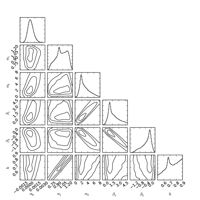
Figure 1: The 1D marginalized distribution, and $1\sigma$, $2\sigma$, $3\sigma$ contours in the 2D model parameter spaces. These results are obtained by fitting the Padé parameterization (6) to SN data. See the text for details.

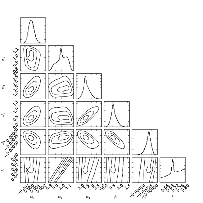
Figure 2: The same as in Fig. 1, except for SN+CMB data.

III $y_{\beta}$-shift cosmography

In this section, we propose another generalization of cosmography inspired by the Padé approximant. We stress that it is completely independent of the one proposed in the previous section. At first, we propose a new $y_{\beta}$-shift inspired by the Padé approximant, and then derive the cosmography of the luminosity distance $d_{L}$ by expanding it as a Taylor series with respect to this new $y_{\beta}$-shift. We will also confront it with the observational data and see whether it works well.

III.1 The formalism of $y_{\beta}$-shift cosmography

At first, we give the motivation to propose the new $y_{\beta}$-shift. As is well known, the standard cosmography of the luminosity distance $d_{L}$ with respect to the redshift $z$ is given by Weinberg2008 ; Visser:2004bf ; Bamba:2012cp ; Dunsby:2015ers ; Chiba:1998tc ; Neben:2012wc  (nb. Eq. (3))

$$\frac{H_{0}d_{L}}{cz}=1+\frac{1}{2}\left(1-q_{0}\right)z+\dots\,.$$ (13)

One can instead parameterize it based on the Padé approximant,

$$\frac{H_{0}d_{L}}{cz}=\frac{\alpha_{0}+\alpha_{1}z+\cdots+\alpha_{m}z^{m}}{1+\beta_{1}z+\cdots+\beta_{n}z^{n}}\,.$$ (14)

Requiring that Eq. (14) coincides with Eq. (13) at $z\to 0$, we find that $\alpha_{0}\to 1$. So, we consider the Padé approximant up to order $(1,\,1)$,

$$\frac{H_{0}d_{L}}{cz}=\frac{1+\alpha z}{1+\beta z}\,.$$ (15)

When $z\ll 1$, Eq. (15) can be expanded as

$$\frac{H_{0}d_{L}}{cz}=1+(\alpha-\beta)z+{\cal O}\left(z^{2}\right)\,.$$ (16)

Comparing it with Eq. (13), we have $\alpha=(1-q_{0})/2+\beta$. So, Eq. (15) becomes

$$\frac{H_{0}d_{L}}{cz}=1+\frac{1}{2}\left(1-q_{0}\right)\frac{z}{1+\beta z}\,.$$ (17)

Putting Eqs. (13) and (17) together, it is quite interesting to see that the quantity $z/(1+\beta z)$ plays a role similar to the redshift $z$. This inspires us to propose a so-called $y_{\beta}$-shift,

$$y_{\beta}\equiv\frac{z}{1+\beta z}\,,$$ (18)

where $\beta$ is a dimensionless constant. Obviously, $y_{\beta}=z$ if $\beta=0$, and $y_{\beta}=z/(1+z)$ if $\beta=1$. Noting that the redshift $z$ Weinberg2008 ; Visser:2004bf ; Bamba:2012cp ; Dunsby:2015ers ; Chiba:1998tc ; Neben:2012wc and $y$-shift $y=z/(1+z)$ Cattoen:2007id ; Cattoen:2008th are extensively used in the usual cosmography, our $y_{\beta}$ can be regarded as their natural generalization. So, the cosmography with respect to $y_{\beta}$-shift is also a natural generalization of the usual cosmography in fact. We stress that the above discussions are only arguments to justify $y_{\beta}$, rather than strict derivations. Now, let us see how it might overcome the problems of the usual cosmography mentioned in Sec. I. First, $y_{\beta}$ is inspired by the Padé approximant, and hence it is well motivated, not purely written by hand. Second, if $1-\beta\ll 1$, we have $y_{\beta}<1$ even for $z\gg 1$. So, the $y_{\beta}$-shift cosmography can converge safely. Third, it can describe the future evolution of the universe, if $1+\beta z\not=0$ in the redshift range $-1<z<0$. In fact, to ensure $y_{\beta}$ remains regular in not only the past but also in the future of the universe ($-1<z<\infty$), it is required that

$$0<\beta<1\,.$$ (19)

In the following, let us derive the cosmography of the luminosity distance $d_{L}$ with respect to $y_{\beta}$-shift. As in e.g. Weinberg2008 ; Visser:2004bf ; Bamba:2012cp ; Dunsby:2015ers ; Chiba:1998tc ; Neben:2012wc ; Cattoen:2007id ; Cattoen:2008th , it is convenient to introduce the following functions,

$$H(t) \equiv +\frac{1}{a}\frac{da}{dt}\,,$$ (20)

$$q(t) \equiv -\frac{1}{aH^{2}}\frac{d^{2}a}{dt^{2}}\,,$$ (21)

$$j(t) \equiv +\frac{1}{aH^{3}}\frac{d^{3}a}{dt^{3}}\,,$$ (22)

$$s(t) \equiv +\frac{1}{aH^{4}}\frac{d^{4}a}{dt^{4}}\,,$$ (23)

$$l(t) \equiv +\frac{1}{aH^{5}}\frac{d^{5}a}{dt^{5}}\,,$$ (24)

which are usually referred to as the Hubble, deceleration, jerk, snap, and lerk parameters. Using these definitions, the Taylor series expansion of scale factor $a$ up to 5th order around the time $t_{0}$ reads

$$\begin{split}a(t)&=a(t_{0})\left[1+H_{0}(t-t_{0})-\frac{q_{0}}{2}H_{0}^{2}(t-t_{0})^{2}+\frac{j_{0}}{3!}H_{0}^{3}(t-t_{0})^{3}\right.\\ &\left.\quad+\frac{s_{0}}{4!}H_{0}^{4}(t-t_{0})^{4}+\frac{l_{0}}{5!}H_{0}^{5}(t-t_{0})^{5}+\mathcal{O}\left((t-t_{0})^{6}\right)\right]\,,\end{split}$$ (25)

where the subscript “0” indicates the value of the corresponding quantity evaluated at the time $t_{0}$. The physical distance traveled by a photon that is emitted at the time $t$ and absorbed at the current epoch $t_{0}$ is given by

$$D=c\int d\tilde{t}=c\left(t_{0}-t\right)\,,$$ (26)

where the time difference $\delta t=t_{0}-t$ is called the “lookback time”. So, we have

$$1+z=\frac{a(t_{0})}{a(t)}=\frac{a(t_{0})}{a(t_{0}-\delta t)}=\frac{a(t_{0})}{a(t_{0}-D/c)}\,.$$ (27)

Using Eq. (25), its right-hand side can be expanded as a Taylor series with respect to $H_{0}D/c\,$,

$$\frac{a(t_{0})}{a(t_{0}-D/c)} =1+\frac{H_{0}D}{c}+\left(1+\frac{1}{2}q_{0}\right)\left(\frac{H_{0}D}{c}\right)^{2}+\left(1+q_{0}+\frac{1}{6}j_{0}\right)\left(\frac{H_{0}D}{c}\right)^{3}$$

$$+\left(1+\frac{3}{2}q_{0}+\frac{1}{4}q_{0}^{2}+\frac{1}{3}j_{0}-\frac{1}{24}s_{0}\right)\left(\frac{H_{0}D}{c}\right)^{4}$$

$$+\left(1+2q_{0}+\frac{3}{4}q_{0}^{2}+\frac{1}{6}q_{0}j_{0}+\frac{1}{2}j_{0}-\frac{1}{12}s_{0}+\frac{1}{120}l_{0}\right)\left(\frac{H_{0}D}{c}\right)^{5}+\mathcal{O}\left(\left(\frac{H_{0}D}{c}\right)^{6}\right)\,.$$ (28)

Therefore, from Eqs. (27) and (28), we obtain

$$\begin{split}z(D)=\mathcal{Z}_{D}^{(1)}\left(\frac{H_{0}D}{c}\right)&+\mathcal{Z}_{D}^{(2)}\left(\frac{H_{0}D}{c}\right)^{2}+\mathcal{Z}_{D}^{(3)}\left(\frac{H_{0}D}{c}\right)^{3}\\ &+\mathcal{Z}_{D}^{(4)}\left(\frac{H_{0}D}{c}\right)^{4}+\mathcal{Z}_{D}^{(5)}\left(\frac{H_{0}D}{c}\right)^{5}+\mathcal{O}\left(\left(\frac{H_{0}D}{c}\right)^{6}\right)\,,\end{split}$$ (29)

where

$$\mathcal{Z}_{D}^{(1)}=1\,,$$ (30)

$$\mathcal{Z}_{D}^{(2)}=1+\frac{1}{2}q_{0}\,,$$ (31)

$$\mathcal{Z}_{D}^{(3)}=1+q_{0}+\frac{1}{6}j_{0}\,,$$ (32)

$$\mathcal{Z}_{D}^{(4)}=1+\frac{3}{2}q_{0}+\frac{1}{4}q_{0}^{2}+\frac{1}{3}j_{0}-\frac{1}{24}s_{0}\,,$$ (33)

$$\mathcal{Z}_{D}^{(5)}=1+2q_{0}+\frac{3}{4}q_{0}^{2}+\frac{1}{6}q_{0}j_{0}+\frac{1}{2}j_{0}-\frac{1}{12}s_{0}+\frac{1}{120}l_{0}\,.$$ (34)

We can expand $D$ as a Taylor series up to 5th order with respect to $y_{\beta}$,

$$D(y_{\beta})=\frac{c}{H_{0}}\left[\mathcal{D}_{y}^{(1)}y_{\beta}+\mathcal{D}_{y}^{(2)}y_{\beta}^{2}+\mathcal{D}_{y}^{(3)}y_{\beta}^{3}+\mathcal{D}_{y}^{(4)}y_{\beta}^{4}+\mathcal{D}_{y}^{(5)}y_{\beta}^{5}+\mathcal{O}\left(y_{\beta}^{6}\right)\right]\,,$$ (35)

in which we have used $D(y_{\beta}=0)=D(t=t_{0})=0$ from Eq. (26). Substituting Eq. (35) into Eq. (29), and using $z=y_{\beta}/(1-\beta y_{\beta})$ obtained from Eq. (18), we have

$$\begin{split}\frac{y_{\beta}}{1-\beta y_{\beta}}&=\mathcal{Z}_{D}^{(1)}\left(\mathcal{D}_{y}^{(1)}y_{\beta}+\mathcal{D}_{y}^{(2)}y_{\beta}^{2}+\mathcal{D}_{y}^{(3)}y_{\beta}^{3}+\mathcal{D}_{y}^{(4)}y_{\beta}^{4}+\mathcal{D}_{y}^{(5)}y_{\beta}^{5}+\mathcal{O}\left(y_{\beta}^{6}\right)\right)\\ &\quad+\mathcal{Z}_{D}^{(2)}\left(\mathcal{D}_{y}^{(1)}y_{\beta}+\mathcal{D}_{y}^{(2)}y_{\beta}^{2}+\mathcal{D}_{y}^{(3)}y_{\beta}^{3}+\mathcal{D}_{y}^{(4)}y_{\beta}^{4}+\mathcal{D}_{y}^{(5)}y_{\beta}^{5}+\mathcal{O}\left(y_{\beta}^{6}\right)\right)^{2}\\ &\quad+\mathcal{Z}_{D}^{(3)}\left(\mathcal{D}_{y}^{(1)}y_{\beta}+\mathcal{D}_{y}^{(2)}y_{\beta}^{2}+\mathcal{D}_{y}^{(3)}y_{\beta}^{3}+\mathcal{D}_{y}^{(4)}y_{\beta}^{4}+\mathcal{D}_{y}^{(5)}y_{\beta}^{5}+\mathcal{O}\left(y_{\beta}^{6}\right)\right)^{3}\\ &\quad+\mathcal{Z}_{D}^{(4)}\left(\mathcal{D}_{y}^{(1)}y_{\beta}+\mathcal{D}_{y}^{(2)}y_{\beta}^{2}+\mathcal{D}_{y}^{(3)}y_{\beta}^{3}+\mathcal{D}_{y}^{(4)}y_{\beta}^{4}+\mathcal{D}_{y}^{(5)}y_{\beta}^{5}+\mathcal{O}\left(y_{\beta}^{6}\right)\right)^{4}\\ &\quad+\mathcal{Z}_{D}^{(5)}\left(\mathcal{D}_{y}^{(1)}y_{\beta}+\mathcal{D}_{y}^{(5)}y_{\beta}^{2}+\mathcal{D}_{y}^{(3)}y_{\beta}^{3}+\mathcal{D}_{y}^{(4)}y_{\beta}^{4}+\mathcal{D}_{y}^{(5)}y_{\beta}^{5}+\mathcal{O}\left(y_{\beta}^{6}\right)\right)^{5}\,.\\ \end{split}$$ (36)

After some algebra, Eq. (36) becomes

$$0 =\left(\mathcal{D}_{y}^{(1)}-1\right)y_{\beta}+\left[\mathcal{D}_{y}^{(2)}-\beta\mathcal{D}_{y}^{(1)}+\left(\mathcal{D}_{y}^{(1)}\right)^{2}\mathcal{Z}_{D}^{(2)}\right]y_{\beta}^{2}$$

$$\quad+\left\{\mathcal{D}_{y}^{(3)}-\beta\mathcal{D}_{y}^{(2)}+\mathcal{Z}_{D}^{(2)}\left[2\mathcal{D}_{y}^{(1)}\mathcal{D}_{y}^{(2)}-\beta\left(\mathcal{D}_{y}^{(1)}\right)^{2}\right]+\mathcal{Z}_{D}^{(3)}\left(\mathcal{D}_{y}^{(1)}\right)^{3}\right\}y_{\beta}^{3}$$

$$\quad+\left\{\mathcal{D}_{y}^{(4)}-\beta\mathcal{D}_{y}^{(3)}+\mathcal{Z}_{D}^{(2)}\left[\left(\mathcal{D}_{y}^{(2)}\right)^{2}+2\mathcal{D}_{y}^{(1)}\mathcal{D}_{y}^{(3)}-2\beta\mathcal{D}_{y}^{(1)}\mathcal{D}_{y}^{(2)}\right]\right.$$

$$\quad\quad\left.+\mathcal{Z}_{D}^{(3)}\left[3\left(\mathcal{D}_{y}^{(1)}\right)^{2}\mathcal{D}_{y}^{(2)}-\beta\left(\mathcal{D}_{y}^{(1)}\right)^{3}\right]+\mathcal{Z}_{D}^{(4)}\left(\mathcal{D}_{y}^{(1)}\right)^{4}\right\}y_{\beta}^{4}$$

$$\quad+\left\{\mathcal{D}_{y}^{(5)}-\beta\mathcal{D}_{y}^{(4)}+\mathcal{Z}_{D}^{(2)}\left[2\left(\mathcal{D}_{y}^{(2)}\mathcal{D}_{y}^{(3)}+\mathcal{D}_{y}^{(1)}\mathcal{D}_{y}^{(4)}\right)-\beta\left(\left(\mathcal{D}_{y}^{(2)}\right)^{2}+2\mathcal{D}_{y}^{(1)}\mathcal{D}_{y}^{(3)}\right)\right]\right.$$

$$\quad\quad+3\mathcal{Z}_{D}^{(3)}\left[\mathcal{D}_{y}^{(1)}\left(\mathcal{D}_{y}^{(2)}\right)^{2}+\left(\mathcal{D}_{y}^{(1)}\right)^{2}\mathcal{D}_{y}^{(3)}-\beta\left(\mathcal{D}_{y}^{(1)}\right)^{2}\mathcal{D}_{y}^{(2)}\right]$$

$$\quad\quad\left.+\mathcal{Z}_{D}^{(4)}\left(\mathcal{D}_{y}^{(1)}\right)^{3}\left(4\mathcal{D}_{y}^{(2)}-\beta\mathcal{D}_{y}^{(1)}\right)+\mathcal{Z}_{D}^{(5)}\left(\mathcal{D}_{y}^{(1)}\right)^{5}\right\}y_{\beta}^{5}+\mathcal{O}\left(y_{\beta}^{6}\right)\,,$$ (37)

in which we have used ${\cal Z}_{D}^{(1)}=1$ from Eq. (30). Requiring all the coefficients of $y_{\beta}^{i}$ in Eq. (37) to be zero, and using Eqs. (31)—(34), we find that

$$\mathcal{D}_{y}^{(1)} =1\,,$$ (38)

$$\mathcal{D}_{y}^{(2)} =-\left(1+\frac{1}{2}q_{0}-\beta\right)\,,$$ (39)

$$\mathcal{D}_{y}^{(3)} =(\beta-1)^{2}-\left(\beta-1\right)q_{0}+\frac{1}{2}q_{0}^{2}-\frac{1}{6}j_{0}\,,$$ (40)

$$\mathcal{D}_{y}^{(4)} =-1+3\beta-3\beta^{2}+\beta^{3}-\left(\frac{3}{2}\beta^{2}-3\beta+\frac{3}{2}\right)q_{0}-\frac{3}{2}\left(1-\beta\right)q_{0}^{2}$$

$$\quad-\frac{5}{8}q_{0}^{3}+\frac{5}{12}q_{0}j_{0}-\frac{1}{2}\left(\beta-1\right)j_{0}+\frac{1}{24}s_{0}\,,$$ (41)

$$\mathcal{D}_{y}^{(5)} =1-4\beta+6\beta^{2}-4\beta^{3}+\beta^{4}+2\left(1-3\beta+3\beta^{2}-\beta^{3}\right)q_{0}+3\left(1-2\beta+\beta^{2}\right)q_{0}^{2}$$

$$\quad+\frac{5}{2}\left(1-\beta\right)q_{0}^{3}+\frac{7}{8}q_{0}^{2}j_{0}+\frac{5}{3}\left(\beta-1\right)q_{0}j_{0}-(\beta-1)^{2}j_{0}$$

$$\quad+\frac{1}{12}j_{0}^{2}+\frac{1}{6}\left(\beta-1\right)s_{0}-\frac{1}{8}q_{0}s_{0}-\frac{1}{120}l_{0}\,.$$ (42)

The role of the observable physical quantity is played by the luminosity distance. Let the photon be emitted at $r$-coordinate $r=0$ at the time $t$, and absorbed at $r$-coordinate $r=r_{0}$ at the time $t_{0}$. Then, the luminosity distance $d_{L}$ is given by (see e.g. the textbooks in Weinberg2008 )

$$d_{L}=\frac{a(t_{0})}{a(t_{0}-D/c)}\,\left(a(t_{0})\,r_{0}\right)\,.$$ (43)

To calculate $d_{L}(D)$, we need $r_{0}(D)$. From Eq. (1), it is easy to obtain Visser:2004bf ; Weinberg2008

$$r_{0}(D)=\begin{cases}\displaystyle\sin\left(\int_{t_{0}-D/c}^{t_{0}}\,\frac{c\,dt}{a(t)}\right)&\ {\rm for}\ \ k=+1\,,\\ &\\ \displaystyle\int_{t_{0}-D/c}^{t_{0}}\,\frac{c\,dt}{a(t)}&\ {\rm for}\ \ k=0\,,\\ &\\ \displaystyle\sinh\left(\int_{t_{0}-D/c}^{t_{0}}\,\frac{c\,dt}{a(t)}\right)&\ {\rm for}\ \ k=-1\,.\end{cases}$$ (44)

Using Eq. (25), we can calculate the integration Bamba:2012cp

$$\int_{t_{0}-D/c}^{t_{0}}\,\frac{c\,dt}{a(t)} =\frac{D}{a_{0}}\left\{1+\frac{1}{2}\left(\frac{H_{0}D}{c}\right)+\frac{1}{6}\left(2+q_{0}\right)\left(\frac{H_{0}D}{c}\right)^{2}+\frac{1}{24}\Big{[}6\big{(}1+q_{0}\big{)}+j_{0}\Big{]}\left(\frac{H_{0}D}{c}\right)^{3}\right.$$

$$\quad+\left.\frac{1}{120}\left(24+36q_{0}+6q_{0}^{2}+8j_{0}-s_{0}\right)\left(\frac{H_{0}D}{c}\right)^{4}+\mathcal{O}\left(\left(\frac{H_{0}D}{c}\right)^{5}\right)\right\}\,,$$ (45)

where $a_{0}=a(t_{0})$. At first glance, we should deal with three cases with space curvature $k=+1$, $0$, $-1$ separately. Fortunately, we need not to do so. As is well known, the Taylor series expansions of $\sin x$ and $\sinh x$ are given by $\sin x=x-x^{3}/3!+x^{5}/5!-x^{7}/7!+\dots$ and $\sinh x=x+x^{3}/3!+x^{5}/5!+x^{7}/7!+\dots$, respectively. Noting that $r_{0}(D)\to\sin(\ast)$ for $k=+1$, and $r_{0}(D)\to\sinh(\ast)$ for $k=-1$, we can write the Taylor series expansion of $r_{0}(D)$ in Eq. (44) as a uniform expression for $k=+1$, $0$, $-1$, i.e. Bamba:2012cp ; Visser:2004bf

$$r_{0}(D)=\left(\int_{t_{0}-D/c}^{t_{0}}\,\frac{c\,dt}{a(t)}\right)-\frac{k}{3!}\left(\int_{t_{0}-D/c}^{t_{0}}\,\frac{c\,dt}{a(t)}\right)^{3}+\frac{k^{2}}{5!}\left(\int_{t_{0}-D/c}^{t_{0}}\,\frac{c\,dt}{a(t)}\right)^{5}+{\cal O}\left(\left(\int_{t_{0}-D/c}^{t_{0}}\,\frac{c\,dt}{a(t)}\right)^{7}\right).$$ (46)

Substituting Eq. (45) into Eq. (46), we have

$$r_{0}(D) =\frac{D}{a_{0}}\left\{1+\frac{1}{2}\left(\frac{H_{0}D}{c}\right)+\frac{1}{6}\left(2+q_{0}-\frac{kc^{2}}{H_{0}^{2}a_{0}^{2}}\right)\left(\frac{H_{0}D}{c}\right)^{2}\right.+\frac{1}{24}\left[6\left(1+q_{0}\right)+j_{0}-\frac{6kc^{2}}{H_{0}^{2}a_{0}^{2}}\right]\left(\frac{H_{0}D}{c}\right)^{3}$$

$$\quad+\frac{1}{120}\left[24+36q_{0}+6q_{0}^{2}+8j_{0}-s_{0}-\frac{5kc^{2}\left(7+2q_{0}\right)}{H_{0}^{2}a_{0}^{2}}+\left(\frac{kc^{2}}{H_{0}^{2}a_{0}^{2}}\right)^{2}\right]\left(\frac{H_{0}D}{c}\right)^{4}$$

$$\quad+\left.\mathcal{O}\left(\left(\frac{H_{0}D}{c}\right)^{5}\right)\right\}\,.$$ (47)

Substituting Eqs. (28), (47), (35) with (38)—(42) into Eq. (43), we finally obtain the cosmography of the luminosity distance $d_{L}$ with respect to $y_{\beta}$-shift,

$$d_{L}(y_{\beta})=\frac{c}{H_{0}}\Big{[}\mathcal{D}_{L}^{(1)}\,y_{\beta}+\mathcal{D}_{L}^{(2)}\,y_{\beta}^{2}+\mathcal{D}_{L}^{(3)}\,y_{\beta}^{3}+\mathcal{D}_{L}^{(4)}\,y_{\beta}^{4}+\mathcal{D}_{L}^{(5)}\,y_{\beta}^{5}+\mathcal{O}\left(y_{\beta}^{6}\right)\Big{]}\,,$$ (48)

where

$$\mathcal{D}_{L}^{(1)} =1\,,$$ (49)

$$\mathcal{D}_{L}^{(2)} =\frac{1}{2}\left(1-q_{0}\right)+\beta\,,$$ (50)

$$\mathcal{D}_{L}^{(3)} =-\frac{1}{6}+\beta+\beta^{2}+\left(\frac{1}{6}-\beta\right)q_{0}+\frac{1}{2}q_{0}^{2}-\frac{1}{6}j_{0}-\frac{1}{6}\left(\frac{kc^{2}}{H_{0}^{2}a_{0}^{2}}\right)\,,$$ (51)

$$\mathcal{D}_{L}^{(4)} =\frac{1}{12}-\frac{1}{2}\beta+\frac{3}{2}\beta^{2}+\beta^{3}+\left(\frac{1}{2}\beta-\frac{3}{2}\beta^{2}-\frac{1}{12}\right)q_{0}+\left(\frac{3}{2}\beta-\frac{5}{8}\right)q_{0}^{2}-\frac{5}{8}q_{0}^{3}$$

$$\quad+\frac{5}{12}q_{0}j_{0}+\left(\frac{5}{24}-\frac{1}{2}\beta\right)j_{0}+\frac{1}{24}s_{0}+\frac{1}{12}\left(1+3q_{0}-6\beta\right)\left(\frac{kc^{2}}{H_{0}^{2}a_{0}^{2}}\right)\,,$$ (52)

$$\mathcal{D}_{L}^{(5)} =-\frac{1}{20}+\frac{1}{3}\beta-\beta^{2}+2\beta^{3}+\beta^{4}+\left(\frac{1}{20}-\frac{1}{3}\beta+\beta^{2}-2\beta^{3}\right)q_{0}$$

$$\quad+\left(\frac{27}{40}-\frac{5}{2}\beta+3\beta^{2}\right)q_{0}^{2}+\left(\frac{11}{8}-\frac{5}{2}\beta\right)q_{0}^{3}+\frac{7}{8}q_{0}^{4}+\left(\frac{5}{3}\beta-\frac{11}{12}\right)q_{0}j_{0}$$

$$\quad-\frac{7}{8}q_{0}^{2}j_{0}+\left(\frac{5}{6}\beta-\beta^{2}-\frac{9}{40}\right)j_{0}+\frac{1}{12}j_{0}^{2}+\left(\frac{1}{6}\beta-\frac{11}{120}\right)s_{0}-\frac{1}{8}q_{0}s_{0}-\frac{1}{120}l_{0}$$

$$\quad-\frac{1}{24}\left(1+8q_{0}+9q_{0}^{2}-2j_{0}-8\beta-24\beta q_{0}+24\beta^{2}\right)\left(\frac{kc^{2}}{H_{0}^{2}a_{0}^{2}}\right)+\frac{1}{120}\left(\frac{kc^{2}}{H_{0}^{2}a_{0}^{2}}\right)^{2}\,.$$ (53)

One can check that if $\beta=0$ or $\beta=1$, these results reduce to the one of cosmography with respect to redshift $z$ (e.g. Bamba:2012cp ; Visser:2004bf ) or $y$-shift $y=z/(1+z)$ (e.g. Cattoen:2007id ; Cattoen:2008th ; Bamba:2012cp ; Vitagliano:2009et ), respectively. The cosmography with respect to $y_{\beta}$-shift $y_{\beta}=z/(1+\beta z)$ obtained here is more general.

III.2 Cosmological constraints from the observational data

It is natural to confront our new cosmography with the observational data, and see whether this new

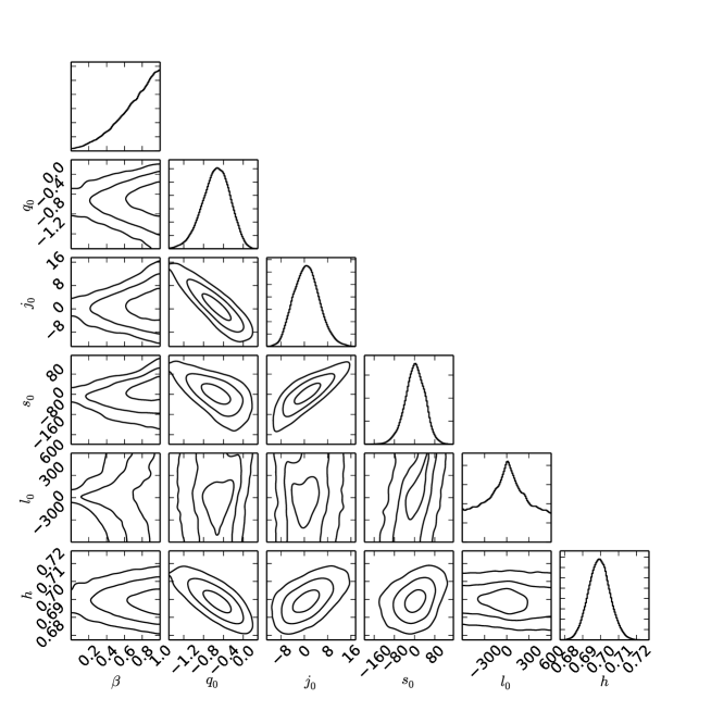
Figure 3: The 1D marginalized distribution, and $1\sigma$, $2\sigma$, $3\sigma$ contours in the 2D model parameter spaces. These results are obtained by fitting the $y_{\beta}$-shift cosmography (48) to SN data with the prior $0<\beta<1$. See the text for details.

cosmography works well. Here, we only consider a flat FRW universe with

$$k=0\,.$$ (54)

Similar to Sec. II, we first consider the constraints from the Union2.1 SNIa dataset Suzuki:2011hu . The $\chi^{2}$ from 580 Union2.1 SNIa is given in Eq. (8), in which $\mu_{th}$ is given by Eq. (7), $D_{L}\equiv H_{0}d_{L}/c$ and $d_{L}$ is given by Eq. (48) in our case. Again, we use the MCMC code emcee ForemanMackey:2012ig to find the best fits and the corresponding $68.3\%$, $95.4\%$ and $99.7\%$ confidence levels to SN data. Note that the prior $0<\beta<1$ is required in Eq. (19). We present the best-fit parameters with $1\sigma$, $2\sigma$, $3\sigma$ uncertainties and the corresponding $\chi^{2}_{min}$ in Table 2. The 1D marginalized distribution, and $1\sigma$, $2\sigma$, $3\sigma$ contours in the 2D model parameter spaces are also given in Fig. 3. It is easy to see that the parameter $\beta$ cannot be well constrained, and its 1D marginalized distribution is not Gaussian. So, we temporarily relax the prior to $0<\beta<2$. In this case, the best-fit parameters with $1\sigma$, $2\sigma$, $3\sigma$ uncertainties and the corresponding $\chi^{2}_{min}$ are given in the last column of Table 2, while the 1D marginalized distribution, and $1\sigma$, $2\sigma$, $3\sigma$ contours in the 2D model parameter spaces are also given in Fig. 4. Now, the constraint on $\beta$ looks well. The following discussions hold for both cases with $0<\beta<1$ and $0<\beta<2$ in fact. It is easy to see that SN data favor a best-fit $\beta$ close to $1$, and hence $y_{\beta}$ is close to the usual $y$-shift $y=z/(1+z)$. However, $\beta$ can still significantly deviate from $1$ in the wide $1\sigma$, $2\sigma$, $3\sigma$ regions. In particular, $\beta$ can even be close to $0$ in the $3\sigma$ region. On the other hand, we find that $q_{0}<0$ at $1\sigma$ confidence level, which indicates the cosmic expansion is accelerating (nb. the definition in Eq. (21)). Of course, it is not surprising that the constraints on $l_{0}$ and $s_{0}$ are fairly loose, since we use only SN data here.

Let us further consider the constraints from the combined SN+CMB data. The corresponding $\chi^{2}$ is given by Eq. (12), in which $\chi^{2}_{SN}$ is given by Eq. (8) and $\chi^{2}_{CMB}=(R-R_{obs})^{2}/\sigma_{R}^{2}$, while $D_{L}\equiv H_{0}d_{L}/c$ and $d_{L}$ is given by Eq. (48) in our case. Note that the prior $0<\beta<1$ is still required in Eq. (19). We present the best-fit parameters with $1\sigma$, $2\sigma$, $3\sigma$ uncertainties and the corresponding $\chi^{2}_{min}$ in Table 3. The 1D marginalized distribution, and $1\sigma$, $2\sigma$, $3\sigma$ contours in the 2D model parameter spaces are also given in Fig. 5. Obviously, the constraints on all parameters are significantly tightened, mainly thanks to the CMB data. It is interesting to see that the combined SN+CMB data favor a best-fit $\beta$ close to $0$, and hence $y_{\beta}$ is close to the usual redshift $z$. Noting that SN data favors a best-fit $\beta$ close to $1$ as mentioned above, this indicates that there is tension between the SN and the CMB data. However, we stress that the constraints from SN and SN+CMB data are still consistent within the $3\sigma$ confidence level. On the other hand, we see that $q_{0}<0$, $j_{0}>0$ beyond $3\sigma$ confidence level, which strongly indicates the cosmic expansion is accelerating, and the acceleration is increasing (nb. the definitions in Eqs. (21) and (22)).

Dataset	SN ($0<\beta<1$)	SN ($0<\beta<2$)
$\chi^{2}_{min}$	565.317	564.668
$\chi^{2}_{min}/dof$	0.985	0.984
$\beta$	$<1$	$0.94516_{-0.42111}^{+0.21990}\,(1\sigma)\,_{-0.75642}^{+0.44858}\,(2\sigma)\,_{-0.92425}^{+0.63060}\,(3\sigma)$
$h$	$0.69932_{-0.00600}^{+0.00589}\,(1\sigma)\,_{-0.01170}^{+0.01221}\,(2\sigma)\,_{-0.01709}^{+0.01819}\,(3\sigma)$	$0.69818_{-0.00581}^{+0.00682}\,(1\sigma)\,_{-0.01208}^{+0.01338}\,(2\sigma)\,_{-0.01847}^{+0.01938}\,(3\sigma)$
$q_{0}$	$-0.55618_{-0.26980}^{+0.28353}\,(1\sigma)\,_{-0.57862}^{+0.50908}\,(2\sigma)_{-0.85393}^{+0.68637}\,(3\sigma)$	$-0.52943_{-0.32969}^{+0.34475}\,(1\sigma)\,_{-0.67578}^{+0.65817}\,(2\sigma)\,_{-0.91769}^{+1.01555}\,(3\sigma)$
$j_{0}$	$0.55909_{-4.21374}^{+4.59544}\,(1\sigma)_{-7.76870}^{+9.48256}\,(2\sigma)_{-11.10038}^{+14.08874}\,(3\sigma)$	$0.39037_{-5.56827}^{+6.47105}\,(1\sigma)\,_{-11.19167}^{+13.46629}\,(2\sigma)\,_{-16.72432}^{+17.82005}\,(3\sigma)$
$s_{0}$	$1.90756_{-39.1773}^{+38.9127}\,(1\sigma)_{-87.1962}^{+75.4962}\,(2\sigma)_{-151.8190}^{+116.3544}\,(3\sigma)$	$3.97831_{-52.4932}^{+63.2142}\,(1\sigma)\,_{-127.5164}^{+145.1346}\,(2\sigma)\,_{-191.6690}^{+191.0794}\,(3\sigma)$
$l_{0}$	$-6.32885_{-342.262}^{+344.384}\,(1\sigma)_{-554.510}^{+563.219}\,(2\sigma)\,_{-591.835}^{+604.266}\,(3\sigma)$	$0.02741_{-360.915}^{+357.489}\,(1\sigma)\,_{-562.618}^{+562.259}\,(2\sigma)\,_{-597.821}^{+597.730}\,(3\sigma)$

Table 2: The best-fit model parameters with $1\sigma$, $2\sigma$, $3\sigma$ uncertainties. The corresponding $\chi^{2}_{min}$ and $\chi^{2}_{min}/dof$ are also given. These results are obtained by fitting the $y_{\beta}$-shift cosmography (48) to SN data with the priors $0<\beta<1$ and $0<\beta<2$, respectively. See the text for details.

Dataset	SN+CMB
$\chi^{2}_{min}$	562.654
$\chi^{2}_{min}/dof$	0.979
$\beta$	$0.13891_{-0.01202}^{+0.01050}\,(1\sigma)\,_{-0.03229}^{+0.02126}\,(2\sigma)\,_{-0.05907}^{+0.03294}\,(3\sigma)$
$h$	$0.70236_{-0.00556}^{+0.00611}\,(1\sigma)\,_{-0.01938}^{+0.01844}\,(2\sigma)\,_{-0.07461}^{+0.07016}\,(3\sigma)$
$q_{0}$	$-0.70925_{-0.07971}^{+0.09912}\,(1\sigma)\,_{-0.19356}^{+0.27603}\,(2\sigma)_{-0.27210}^{+0.55496}\,(3\sigma)$
$j_{0}$	$1.98747_{-0.35293}^{+0.31463}\,(1\sigma)_{-0.92251}^{+1.03983}\,(2\sigma)_{-1.50048}^{+2.07407}\,(3\sigma)$
$s_{0}$	$0.69908_{-1.11125}^{+0.99476}\,(1\sigma)_{-3.04250}^{+3.71175}\,(2\sigma)_{-6.00546}^{+7.70008}\,(3\sigma)$
$l_{0}$	$-1.31401_{-3.56927}^{+3.29455}\,(1\sigma)_{-12.98544}^{+17.06251}\,(2\sigma)\,_{-35.29680}^{+38.88782}\,(3\sigma)$

Table 3: The same as in Table 2, except for SN+CMB data and the prior $0<\beta<1$ only.

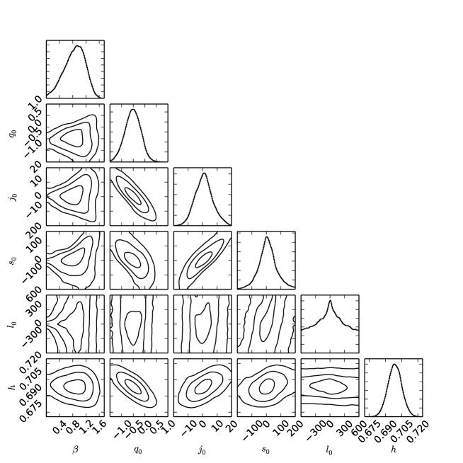
Figure 4: The same as in Fig. 3, except for the prior $0<\beta<2$.

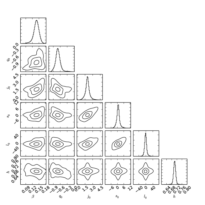
Figure 5: The same as in Fig. 3, except for SN+CMB data, and the prior $0<\beta<1$ is required.

IV Concluding remarks

The current accelerated expansion of the universe has been one of the most important fields in physics and astronomy since 1998. Many cosmological models have been proposed in the literature to explain this mysterious phenomenon. Since the nature and cause of the cosmic acceleration are still unknown, model-independent approaches to study the evolution of the universe are welcome. One of the powerful model-independent approaches is the so-called cosmography. It only relies on the cosmological principle, without postulating any underlying theoretical model. However, there are several shortcomings in the usual cosmography. In the present work, we try to overcome or at least alleviate these problems, and propose two new generalizations of cosmography inspired by the Padé approximant. We also confront them with the observational data with the help of the Markov chain Monte Carlo (MCMC) code emcee ForemanMackey:2012ig , and find that they work fairly well.

In the literature (e.g. Weinberg2008 ; Visser:2004bf ; Bamba:2012cp ; Dunsby:2015ers ; Chiba:1998tc ; Neben:2012wc ; Cattoen:2007id ; Cattoen:2008th ; Aviles:2012ay ; Capozziello:2008tc ; Vitagliano:2009et ; Luongo:2011zz ; Busti:2015xqa ; Semiz:2015gga ), there exist a number of works on cosmography. They focused on various issues in cosmology and made much significant progress. However, the previous works used ordinary cosmography mainly with respect to the redshift $z$ or the so-called $y$-shift $y=z/(1+z)$. We stress that they are all plagued with the problem of divergence (or the unacceptably large error when $y\sim 1$), and all fail to predict the future evolution of the universe (especially when $z\sim-1$ or $y<-1$), as mentioned in Sec. I. In the present work, the two new generalizations of cosmography proposed in Secs. II and III can instead avoid or at least alleviate these problems of ordinary cosmography. In addition, our new generalizations of cosmography are well motivated by the Padé approximant, rather than written purely by hand. In fact, it has been solidly proved by mathematicians that any (even unknown) function can be well approximated by a Padé approximant r3 ; r4 ; r5 , and the Padé approximant often gives a better approximation of the function than truncating its Taylor series, and it may still work where the Taylor series does not converge r4 . Noting that ordinary cosmography is actually based on a Taylor series, the advantages of the Padé approximant mentioned above make our new generalizations better than the ordinary cosmography used in the literature. Although the Padé approximant has been considered in cosmology (see e.g. Adachi:2011vu ; Gruber:2013wua ; Wei:2013jya ; Liu:2014vda ; padeworks ), here we instead use it in a fairly different issue. For example, in e.g. Wei:2013jya ; Liu:2014vda the Padé approximant was used to study the issues of an analytical approximation of the luminosity distance in the XCDM model, EoS parameterizations, and gamma-ray burst cosmology, while we use it to generalize cosmography in this work. By all the above arguments, we stress that the present work is significantly different from the previous works on both cosmography and the Padé approximant in the literature.

The key to avoid or at least alleviate the problems of ordinary cosmography is the denominator of the Padé approximant. Considering Eqs. (5) or (4), if the order $n$ of the denominator is larger than or equal to the order $m$ of the numerator, this Padé approximant with $n\geq m$ will not diverge even for $z\gg 1$. In fact, this is just the case of our two generalizations (nb. Eqs. (6) and (18)). On the other hand, for suitable parameters $\beta_{i}$, it is easy to ensure the denominator not to equal zero for the very wide redshift range $-1<z<\infty$, and hence the Padé approximant can avoid divergence. The shortcomings of ordinary cosmography mainly have their roots in the Taylor series. So, generalizing a Taylor series to the Padé approximant brings about a possible way out. If all $\beta_{i}=0$ in the denominator of the Padé approximant, it reduces to the usual Taylor series. However, a denominator not equal to $1$ and $0$ makes a big difference.

Here, we would like to clarify the main difference between the two new generalizations proposed in Secs. II and III. Noting that ordinary cosmography is based on a Taylor series, the first one generalizes cosmography by directly generalizing the Taylor series to the Padé approximant when we expand the luminosity distance $d_{L}$ (nb. Eq. (5)). On the other hand, the second one instead generalizes cosmography by generalizing the redshift $z$ or the $y$-shift $y=z/(1+z)$ to the so-called $y_{\beta}$-shift $y_{\beta}=z/(1+\beta z)$ (which is inspired by the Padé approximant), but we still expand the luminosity distance $d_{L}$ in a Taylor series (nb. Eq. (48)), rather than the Padé approximant itself. This is the main difference. Noting that $y_{\beta}=z$ and $z/(1+z)$ when $\beta=0$ and $1$ respectively, we call $y_{\beta}=z/(1+\beta z)$ the “$y_{\beta}$-shift” in analogy to the well-known terminology of the “$y$-shift” $y=z/(1+z)$ used in the literature, while the terminology “$y$-shift” comes from the terminology “red-shift” in fact.

It is of interest to quantitatively compare our two new generalizations of cosmography, and also compare them with the ordinary cosmography (we thank the referee for pointing out this issue). Let us compare our $y_{\beta}$-shift cosmography with the ordinary cosmography first. The observational constraints on our $y_{\beta}$-shift cosmography from the SN+CMB data are presented in Table 3 and Fig. 5. It is easy to see that $\beta=0$ and $\beta=1$ deviate from the best fit far beyond the $3\sigma$ confidence level, see especially the leftmost column of Fig. 5. Note that our $y_{\beta}$-shift reduces to the ordinary redshift $z$ and the $y$-shift $y=z/(1+z)$ when $\beta=0$ and $1$, respectively. Therefore, our $y_{\beta}$-shift cosmography can fit the SN+CMB data significantly better than ordinary cosmography. On the other hand, from the last column of Table 1 and Table 3, $\chi^{2}_{min}=562.171$ and $\chi^{2}_{min}/dof=0.978$ by fitting the Padé parameterization to the SN+CMB data, while $\chi^{2}_{min}=562.654$ and $\chi^{2}_{min}/dof=0.979$ by fitting the $y_{\beta}$-shift cosmography to the SN+CMB data. Therefore, our first generalization of cosmography is slightly better than the second one.

Other remarks are in order. First, the Padé approximant has been used previously in cosmology, e.g. in slow-roll inflation, the reconstruction of the scalar field potential, data fitting and analytical approximation of the luminosity distance, EoS parameterizations, gamma-ray burst cosmology, and cosmological perturbations in LSS (see e.g. Adachi:2011vu ; Gruber:2013wua ; Wei:2013jya ; Liu:2014vda ; padeworks ). We advocate further uses of the Padé approximant in cosmology. Second, in the present work we only derive the generalized cosmography of the luminosity distance $d_{L}$. In fact, one can easily obtain the corresponding cosmography of other observable quantities, such as the angular diameter distance $d_{A}$, the photon flux distance $d_{F}$, the photon count distance $d_{P}$, and the deceleration distance $d_{Q}$, since they can be readily related to the luminosity distance $d_{L}$ (see e.g. Cattoen:2008th ). Third, we confront the generalized cosmography with the observational data only for the spatially flat FRW universe ($k=0$). In fact, one can do this for the $k\not=0$ cases easily, and hence we do not present them here. Finally, the usual cosmography with respect to the redshift $z$ and $y$-shift $y=z/(1+z)$ has been extensively applied to various cosmological issues, for instance, the EoS of dark energy, modified gravity theories like $f(R)$ and $f(T)$ theories, gamma-ray burst cosmology, and so on (see e.g. Weinberg2008 ; Visser:2004bf ; Bamba:2012cp ; Dunsby:2015ers ; Chiba:1998tc ; Neben:2012wc ; Cattoen:2007id ; Cattoen:2008th ; Aviles:2012ay ; Capozziello:2008tc ; Vitagliano:2009et ; Luongo:2011zz ; Busti:2015xqa ; Semiz:2015gga ). The new generalizations of cosmography proposed in the present work can also be used in these cosmological issues, and we leave it to the future works.

References

- (1) A. G. Riess et al., Astron. J. 116, 1009 (1998) [astro-ph/9805201].
- (2) S. Perlmutter et al., Astrophys. J. 517, 565 (1999) [astro-ph/9812133].
- (3) L. Page et al. [WMAP Collaboration], Astrophys. J. Suppl. 148, 233 (2003) [astro-ph/0302220].
- (4) D. N. Spergel et al. [WMAP Collaboration], Astrophys. J. Suppl. 170, 377 (2007) [astro-ph/0603449].
- (5) E. Komatsu et al. [WMAP Collaboration], Astrophys. J. Suppl. 180, 330 (2009) [arXiv:0803.0547].
- (6) E. Komatsu et al. [WMAP Collaboration], Astrophys. J. Suppl. 192, 18 (2011) [arXiv:1001.4538].
- (7) M. Tegmark et al. [SDSS Collaboration], Phys. Rev. D 69, 103501 (2004) [astro-ph/0310723].
- (8) U. Seljak et al. [SDSS Collaboration], Phys. Rev. D 71, 103515 (2005) [astro-ph/0407372].
-
(9)
E. J. Copeland, M. Sami and S. Tsujikawa,
Int. J. Mod. Phys. D 15, 1753 (2006)
[hep-th/0603057];
J. Frieman, M. Turner and D. Huterer, Ann. Rev. Astron. Astrophys. 46, 385 (2008) [arXiv:0803.0982];
S. Tsujikawa, arXiv:1004.1493 [astro-ph.CO];
M. Li et al., Commun. Theor. Phys. 56, 525 (2011) [arXiv:1103.5870];
A. De Felice and S. Tsujikawa, Living Rev. Rel. 13, 3 (2010) [arXiv:1002.4928]. - (10) K. Bamba et al., Astrophys. Space Sci. 342, 155 (2012) [arXiv:1205.3421].
-
(11)
M. Kunz and D. Sapone,
Phys. Rev. Lett. 98, 121301 (2007)
[astro-ph/0612452];
E. Bertschinger and P. Zukin, Phys. Rev. D 78, 024015 (2008) [arXiv:0801.2431]. -
(12)
H. Wei and S. N. Zhang,
Phys. Rev. D 78, 023011 (2008)
[arXiv:0803.3292];
B. Jain and P. Zhang, Phys. Rev. D 78, 063503 (2008) [arXiv:0709.2375];
H. Wei, J. Liu, Z. C. Chen and X. P. Yan, Phys. Rev. D 88, 043510 (2013) [arXiv:1306.1364]. -
(13)
I. Maor, R. Brustein and P. J. Steinhardt,
Phys. Rev. Lett. 86, 6 (2001)
[astro-ph/0007297];
A. G. Riess et al. [Supernova Search Team Collaboration], Astrophys. J. 607, 665 (2004) [astro-ph/0402512]. -
(14)
M. Chevallier and D. Polarski,
Int. J. Mod. Phys. D 10, 213 (2001)
[gr-qc/0009008];
E. V. Linder, Phys. Rev. Lett. 90, 091301 (2003) [astro-ph/0208512]. -
(15)
P. K. S. Dunsby and O. Luongo,
Int. J. Geom. Meth. Mod. Phys. 13, 1630002
(2016) [arXiv:1511.06532];
S. Capozziello, M. De Laurentis, O. Luongo and A. Ruggeri, Galaxies 1, 216 (2013) [arXiv:1312.1825]. - (16) C. Cattoen and M. Visser, Phys. Rev. D 78, 063501 (2008) [arXiv:0809.0537].
-
(17)
S. Weinberg, Gravitation and Cosmology,
John Wiley & Sons, Inc., New York (1972);
S. Weinberg, Cosmology, Oxford University Press, Oxford (2008). -
(18)
M. Visser,
Class. Quant. Grav. 21, 2603 (2004)
[gr-qc/0309109];
M. Visser, Gen. Rel. Grav. 37, 1541 (2005) [gr-qc/0411131]. - (19) T. Chiba and T. Nakamura, Prog. Theor. Phys. 100, 1077 (1998) [astro-ph/9808022].
- (20) A. R. Neben and M. S. Turner, Astrophys. J. 769, 133 (2013) [arXiv:1209.0480].
-
(21)
C. Cattoen and M. Visser,
gr-qc/0703122;
C. Cattoen and M. Visser, Class. Quant. Grav. 24, 5985 (2007) [arXiv:0710.1887];
M. Visser and C. Cattoen, arXiv:0906.5407 [gr-qc]. - (22) A. Aviles, C. Gruber, O. Luongo and H. Quevedo, Phys. Rev. D 86, 123516 (2012) [arXiv:1204.2007].
-
(23)
D. Foreman-Mackey et al.,
Publ. Astron. Soc. Pac. 125, 306 (2013)
[arXiv:1202.3665];
The code emcee is available at http://dan.iel.fm/emcee/current & https://github.com/dfm/emcee -
(24)
H. Padé,
Ann. Sci. Ecole Norm. Sup. 9 (3), 1-93 (1892);
S. G. Krantz and H. R. Parks, A Primer of Real Analytic Functions, Birkhäuser (1992);
G. A. Baker, Jr. and P. Graves-Morris, Padé Approximants, Cambridge University Press (1996). - (25) http:en.wikipedia.org/wiki/Pade-approximant
-
(26)
http:www.scholarpedia.org/article/Pade-approximant
http:www-sop.inria.fr/apics/anap03/PadeTalk.pdf - (27) M. Adachi and M. Kasai, Prog. Theor. Phys. 127, 145 (2012) [arXiv:1111.6396].
-
(28)
C. Gruber and O. Luongo,
Phys. Rev. D 89, 103506 (2014)
[arXiv:1309.3215];
A. Aviles, A. Bravetti, S. Capozziello and O. Luongo, Phys. Rev. D 90, 043531 (2014) [arXiv:1405.6935]. - (29) H. Wei, X. P. Yan and Y. N. Zhou, JCAP 1401, 045 (2014) [arXiv:1312.1117].
- (30) J. Liu and H. Wei, Gen. Rel. Grav. 47, 141 (2015) [arXiv:1410.3960].
-
(31)
N. Suzuki et al.,
Astrophys. J. 746, 85 (2012)
[arXiv:1105.3470];
The numerical data of the full Union2.1 sample are available at http://supernova.lbl.gov/Union -
(32)
S. Nesseris and L. Perivolaropoulos,
Phys. Rev. D 72, 123519 (2005)
[astro-ph/0511040];
L. Perivolaropoulos, Phys. Rev. D 71, 063503 (2005) [astro-ph/0412308]. - (33) E. Di Pietro and J. F. Claeskens, Mon. Not. Roy. Astron. Soc. 341, 1299 (2003) [astro-ph/0207332].
-
(34)
H. Wei, N. N. Tang and S. N. Zhang,
Phys. Rev. D 75, 043009 (2007)
[astro-ph/0612746];
H. Wei and R. G. Cai, Phys. Lett. B 663, 1 (2008) [arXiv:0708.1894];
H. Wei, Phys. Lett. B 687, 286 (2010) [arXiv:0906.0828];
H. Wei, Phys. Lett. B 692, 167 (2010) [arXiv:1005.1445];
H. Wei, JCAP 1104, 022 (2011) [arXiv:1012.0883];
H. Wei, Z. C. Chen and J. Liu, Phys. Lett. B 720, 271 (2013) [arXiv:1302.0643];
Y. Wu, Z. C. Chen, J. Wang and H. Wei, Commun. Theor. Phys. 63, 701 (2015) [arXiv:1503.05281]. - (35) P. A. R. Ade et al. [Planck Collaboration], arXiv:1502.01589 [astro-ph.CO].
- (36) P. A. R. Ade et al. [Planck Collaboration], arXiv:1502.01590 [astro-ph.CO].
-
(37)
J. R. Bond, G. Efstathiou and M. Tegmark,
Mon. Not. Roy. Astron. Soc. 291, L33 (1997)
[astro-ph/9702100];
G. Efstathiou and J. R. Bond, Mon. Not. Roy. Astron. Soc. 304, 75 (1999) [astro-ph/9807103]. - (38) Y. Wang and P. Mukherjee, Astrophys. J. 650, 1 (2006) [astro-ph/0604051].
- (39) Y. Wang and S. Wang, Phys. Rev. D 88, 043522 (2013) [arXiv:1304.4514].
- (40) D. L. Shafer and D. Huterer, Phys. Rev. D 89, 063510 (2014) [arXiv:1312.1688].
- (41) R. G. Cai, Z. K. Guo and B. Tang, Phys. Rev. D 89, 123518 (2014) [arXiv:1312.4309].
-
(42)
A. R. Liddle, P. Parsons and J. D. Barrow,
Phys. Rev. D 50, 7222 (1994)
[astro-ph/9408015];
T. D. Saini et al., Phys. Rev. Lett. 85, 1162 (2000) [astro-ph/9910231];
D. Huterer and M. S. Turner, Phys. Rev. D 64, 123527 (2001) [astro-ph/0012510];
J. Jonsson, A. Goobar, R. Amanullah and L. Bergstrom, JCAP 0409, 007 (2004) [astro-ph/0404468];
D. Blas, M. Garny and T. Konstandin, JCAP 1401, 010 (2014) [arXiv:1309.3308];
A. Yoshisato, T. Matsubara and M. Morikawa, Astrophys. J. 498, 48 (1998) [astro-ph/9707296]. -
(43)
S. Capozziello and L. Izzo,
Astron. Astrophys. 490, 31 (2008)
[arXiv:0806.1120];
S. Capozziello and L. Izzo, Astron. Astrophys. 519, A73 (2010) [arXiv:1003.5319];
V. F. Cardone, M. Perillo and S. Capozziello, Mon. Not. Roy. Astron. Soc. 417, 1672 (2011) [arXiv:1105.1122];
H. Gao, N. Liang and Z. H. Zhu, Int. J. Mod. Phys. D 21, 1250016 (2012) [arXiv:1003.5755]. -
(44)
V. Vitagliano, J. Q. Xia, S. Liberati and M. Viel,
JCAP 1003, 005 (2010)
[arXiv:0911.1249];
J. Q. Xia, V. Vitagliano, S. Liberati and M. Viel, Phys. Rev. D 85, 043520 (2012) [arXiv:1103.0378]. -
(45)
O. Luongo,
Mod. Phys. Lett. A 26, 1459 (2011);
A. Aviles, A. Bravetti, S. Capozziello and O. Luongo, Phys. Rev. D 87, 064025 (2013) [arXiv:1302.4871];
A. Aviles, A. Bravetti, S. Capozziello and O. Luongo, Phys. Rev. D 87, 044012 (2013) [arXiv:1210.5149];
S. Capozziello, M. De Laurentis and O. Luongo, Annalen Phys. 526, 309 (2014) [arXiv:1406.6996];
O. Luongo, G. B. Pisani and A. Troisi, arXiv:1512.07076 [gr-qc]. - (46) V. C. Busti et al., Phys. Rev. D 92, 123512 (2015) [arXiv:1505.05503].
- (47) I. Semiz and A. K. Camlibel, JCAP 1512, 038 (2015) [arXiv:1505.04043].