High-order time stepping for the Navier-Stokes equations with minimal computational complexity

Abstract.

In this paper we present extensions of the schemes proposed in Guermond and Minev [2] that lead to a decoupling of the velocity components in the momentum equation. The new schemes reduce the solution of the incompressible Navier-Stokes equations to a set of classical uncoupled parabolic problems for each Cartesian component of the velocity. The pressure is explicitly recovered after the velocity is computed.

1. Introduction

In Guermond and Minev [2], we considered the possibility to construct high order artificial compressibility schemes for incompressible flow. The resulting schemes require the solution of problems of the type $\mathbf{u}-\nu\tau{\Delta}\mathbf{u}-\tau\nabla\nabla\!{\cdot}\mathbf{u}=\tau{\bf f}$, $\tau$ being the time step. The corresponding discrete problem clearly has a condition number of the order of $\tau h^{-2}$, $h$ being the spatial step. In this paper we consider some possibilities to improve this algorithm by discretizing the $\nabla\nabla\!{\cdot}$ operator in an implicit-explicit fashion in order to decouple the Cartesian components of the velocity and thereby reducing the problem to a series of scalar-valued parabolic problems. In fact, such strategies based on the direction splitting approach, which was popular at that time, have been proposed in the literature in the 1960s and 70s. For instance, a direction splitting scheme that includes the splitting of the $\nabla\nabla\!{\cdot}$ operator has been proposed in the Russian literature by the groups of Yanenko (see Vladimirova et al. [7], Yanenko [8], section 8.3) and Ladizhenskaya ( see Ladyzhenskaya [4], chapter VI, section 9.2, and the references therein). In the Western literature, such schemes have been proposed and analyzed by Temam [5], chapter III, section 8.3. In the present paper we generalize the approach to make it applicable to non-Cartesian grids without splitting, and we combine it with the defect correction approach discussed in Guermond and Minev [2] to increase the order. Furthermore, we propose new direction splitting schemes that allow the use of direct methods for three dimensional problems.

2. Preliminaries

2.1. Formulation of the problem

We consider the time-dependent Navier-Stokes equations on a finite time interval $[0,T]$ and in a domain $\Omega$ in $\mathbb{R}^{d}$ with a Lipschitz boundary. Since the nonlinear term in the Navier-Stokes equations has no significant influence on the pressure-velocity coupling and since this term is usually made explicit, we henceforth mostly consider the time-dependent Stokes equations written in terms of velocity $\boldsymbol{u}$ and pressure $p$:

(2.1) $$\left\{\begin{aligned} &\partial_{t}\boldsymbol{u}+{\mathbb{A}}\boldsymbol{u}+\nabla p={\bf f}\quad\text{in $\Omega\times[0,T]$},\\ &\nabla\!{\cdot}\boldsymbol{u}=0\quad\text{in $\Omega\times[0,T]$},\\ &\boldsymbol{u}|_{\partial\Omega}=0\quad\text{in [0,T]},\quad\text{ and }\boldsymbol{u}|_{t=0}=\boldsymbol{u}_{0}\quad\text{in $\Omega$},\end{aligned}\right.$$

where ${\bf f}$ is a smooth source term and $\boldsymbol{u}_{0}$ is a solenoidal initial velocity field with zero normal trace at the boundary of $\Omega$. The operator ${\mathbb{A}}$ is assumed to be linear, ${\bf H}^{1}$-coercive and bounded, i.e., there are two constants $\nu>0$ and $M<\infty$ such that $\int_{\Omega}{\mathbb{A}}\mathbf{u}{\cdot}\mathbf{u}\,\mbox{\rm d}{\bf x}\geq\nu\|\mathbf{u}\|_{{\bf H}^{1}(\Omega)}^{2}$ and $|\int_{\Omega}{\mathbb{A}}\mathbf{u}{\cdot}{\bf v}\,\mbox{\rm d}{\bf x}|\leq M\|\mathbf{u}\|_{{\bf H}^{1}(\Omega)}\|{\bf v}\|_{{\bf H}^{1}(\Omega)}$, for all $\mathbf{u},{\bf v}\in{\bf H}^{1}_{0}(\Omega)$. For the sake of simplicity, we consider homogeneous Dirichlet boundary conditions on the velocity.

We are going to be mainly concerned with time discretizations of the above problem. Let $\tau>0$ be a time step and set $t^{n}=n\tau$ for $0\leq n\leq N=\lfloor T/\tau\rfloor$, where $\lfloor\cdot\rfloor$ is the floor function. Let $\phi^{0},\phi^{1},\ldots\phi^{N}$ be some sequence of functions in a Hilbert space $E$. We denote by $\phi_{\tau}$ this sequence, and we define the following discrete norms: $\|\phi_{\tau}\|_{\ell^{2}(E)}:=\big{(}\tau\sum_{n=0}^{N}\|\phi^{n}\|_{E}^{2}\big{)}^{\frac{1}{2}}$, $\|\phi_{\tau}\|_{\ell^{\infty}(E)}:=\max_{0\leq n\leq N}\left(\|\phi^{n}\|_{E}\right)$. In addition, we denote the first differences of the elements of the sequence by $\displaystyle\delta_{t}\phi^{n}=(\phi^{n}-\phi^{n-1}),n=1,\dots,N$, and their average $\displaystyle\bar{\phi}^{n}=(\phi^{n}+\phi^{n-1})/2,n=1,\dots,N$. The sequences $\delta_{t}\phi^{1},\ldots\delta_{t}\phi^{N}$ and $\bar{\phi}^{1},\ldots\bar{\phi}^{N}$ are denoted by $\delta_{t}\phi_{\tau}$ and $\bar{\phi}_{\tau}$ correspondingly. We also denote by $c$ a generic constant that is independent of $\tau$ and $\epsilon$ but possibly depends on the data, the domain, and the solution.

2.2. High-order artificial compressibility

In Guermond and Minev [2] we introduced a series of second and third-order schemes based on the following elementary first-order artificial compressibility algorithm:

(2.2) $$\frac{\mathbf{u}^{n+1}-\mathbf{u}^{n}}{\tau}+{\mathbb{A}}\mathbf{u}^{n+1}+\nabla p^{n+1}={\bf f}^{n+1},\quad\frac{\epsilon}{\tau}(p^{n+1}-p^{n})+\nabla\!{\cdot}\mathbf{u}^{n+1}=0,$$

where $\epsilon>0$ is a user-dependent parameter that is usually chosen to be proportional to $\tau$, i.e., $\epsilon=\tau/\chi$ where $\chi$ is of order one. One interesting property of this scheme is that it decouples the velocity and the pressure; more precisely, the algorithm can be recast as follows:

(2.3) $$\frac{\mathbf{u}^{n+1}-\mathbf{u}^{n}}{\tau}+{\mathbb{A}}\mathbf{u}^{n+1}-\chi\nabla\nabla\!{\cdot}\mathbf{u}^{n+1}={\bf f}^{n+1}-\nabla p^{n},\quad p^{n+1}=-p^{n}-\chi\nabla\!{\cdot}\mathbf{u}^{n+1}.$$

The above algorithm has been extended to third-order accuracy in time in [2] by using a defect correction method. Denoting by $B\mathbf{u}$ the nonlinear term in the Navier-Stokes equations, the full third order scheme is as follows:

(2.4) $$n\geq 0,\qquad\begin{cases}\textbf{nl}_{0}^{n+1}=B\mathbf{u}_{0}^{n},\\ \displaystyle\frac{\mathbf{u}_{0}^{n+1}-\mathbf{u}_{0}^{n}}{\tau}+{\mathbb{A}}\mathbf{u}_{0}^{n+1}-\chi\nabla\nabla\!{\cdot}\mathbf{u}_{0}^{n+1}+\nabla p_{0}^{n}={\bf f}^{n+1}-\textbf{nl}_{0}^{n+1}\\ p_{0}^{n+1}=p_{0}^{n}-\chi\nabla\!{\cdot}\mathbf{u}_{0}^{n+1},\\ d\mathbf{u}_{0}^{n+1}=(\mathbf{u}_{0}^{n+1}-\mathbf{u}_{0}^{n})/\tau,\quad dp_{0}^{n+1}=(p_{0}^{n+1}-p_{0}^{n})/\tau\end{cases}$$

(2.5) $$n\geq 1,\qquad\begin{cases}d^{2}\mathbf{u}_{0}^{n+1}=(d\mathbf{u}_{0}^{n+1}-d\mathbf{u}_{0}^{n})/\tau,\\ \textbf{nl}_{1}^{n}=B(\mathbf{u}_{0}^{n}+\tau\mathbf{u}_{1}^{n-1}),\\ \displaystyle\frac{\mathbf{u}_{1}^{n}-\mathbf{u}_{1}^{n-1}}{\tau}+{\mathbb{A}}\mathbf{u}_{1}^{n}-\chi\nabla\nabla\!{\cdot}\mathbf{u}_{1}^{n}+\nabla(p_{1}^{n-1}+dp_{0}^{n})\displaystyle=-\frac{1}{2}d^{2}\mathbf{u}_{0}^{n+1}-\frac{\textbf{nl}_{1}^{n}-\textbf{nl}_{0}^{n}}{\tau},\\ p_{1}^{n}=p_{1}^{n-1}+dp_{0}^{n}-\chi\nabla\!{\cdot}\mathbf{u}_{1}^{n},\\ d\mathbf{u}_{1}^{n}=(\mathbf{u}_{1}^{n}-\mathbf{u}_{1}^{n-1})/\tau,\quad dp_{1}^{n}=(p_{1}^{n}-p_{1}^{n-1})/\tau,\end{cases}$$

(2.6) $$n\geq 2,\quad\begin{cases}d^{2}\mathbf{u}_{1}^{n}=(d\mathbf{u}_{1}^{n}-d\mathbf{u}_{1}^{n-1})/\tau,\qquad d^{3}\mathbf{u}_{0}^{n+1}=(d^{2}\mathbf{u}_{0}^{n+1}-d^{2}\mathbf{u}_{0}^{n})/\tau,\\ \textbf{nl}_{2}^{n-1}=B(\mathbf{u}_{0}^{n-1}+\tau\mathbf{u}_{1}^{n-1}+\tau^{2}\mathbf{u}_{2}^{n-2})\\ \displaystyle\frac{\mathbf{u}_{2}^{n-1}-\mathbf{u}_{2}^{n-2}}{\tau}+{\mathbb{A}}\mathbf{u}_{2}^{n-1}-\chi\nabla\nabla\!{\cdot}\mathbf{u}_{2}^{n-1}+\nabla(p_{2}^{n-2}+dp_{1}^{n-1})\\ \displaystyle\hskip 113.81102pt=-\frac{1}{2}d^{2}\mathbf{u}_{1}^{n}+\frac{1}{6}d^{3}\mathbf{u}_{0}^{n+1}-\frac{\textbf{nl}_{2}^{n-1}-\textbf{nl}_{1}^{n-1}}{\tau^{2}}\\ p_{2}^{n-1}=p_{2}^{n-2}+dp_{1}^{n-1}-\chi\nabla\!{\cdot}\mathbf{u}_{2}^{n-1},\\ \mathbf{u}^{n-1}=\mathbf{u}_{0}^{n-1}+\tau\mathbf{u}_{1}^{n-1}+\tau^{2}\mathbf{u}_{2}^{n-1},\quad p^{n-1}=p_{0}^{n-1}+\tau p_{1}^{n-1}+\tau^{2}p_{2}^{n-1},\end{cases}$$

The stage (2.4) yields a first order approximation of the velocity and the pressure, the second stage (2.5) yields a second order approximation of the velocity and the pressure, and the third stage (2.6) yields a third order approximation of the velocity and the pressure.

One drawback of the above scheme is the presence of the $\nabla\nabla\!{\cdot}$ operator since this operator couples all the Cartesian components of the velocity and can lead to locking if not discretized properly. In the next section we introduce a first order artificial compressibility scheme that decouples the different components of the velocity, i.e., we develop a decoupled version of the first stage (2.4). We will use this approach later in the paper to modify the subsequent two stages and create a high-order time stepping for the Navier-Stokes equations that requires only the solution of a set of scalar-valued parabolic problems for each Cartesian component of the velocity. Since the proofs of stability of these schemes in two and three dimensions differ somewhat, we will consider these two cases separately.

3. Splitting of the grad-div operator

3.1. Splitting of ${\mathbb{A}}$

To be general we are going to assume that the operator ${\mathbb{A}}$ admits the following decomposition ${\mathbb{A}}\mathbf{u}=Au-\nabla(\lambda\nabla\!{\cdot}\mathbf{u})$ where $\lambda$ is a smooth positive scalar field. We assume also that $A$ is block diagonal, ${\bf H}^{1}$-coercive and bounded, i.e., $A\mathbf{u}=(A_{1}u_{1},\ldots,A_{d}u_{d})^{\sf T}$, $\int_{\Omega}A\mathbf{u}{\cdot}\mathbf{u}\,\mbox{\rm d}{\bf x}\geq\nu\|\mathbf{u}\|_{{\bf H}^{1}(\Omega)}^{2}$ and $|\int_{\Omega}A\mathbf{u}{\cdot}{\bf v}\,\mbox{\rm d}{\bf x}|\leq M\|\mathbf{u}\|_{{\bf H}^{1}(\Omega)}\|{\bf v}\|_{{\bf H}^{1}(\Omega)}$, for all $\mathbf{u},{\bf v}\in{\bf H}^{1}_{0}(\Omega)$, where $u_{1},\ldots,u_{d}$ are the Cartesian components of $\mathbf{u}$. This decomposition holds for instance when ${\mathbb{A}}\mathbf{u}=-\nabla\!{\cdot}(\mu(\nabla\mathbf{u}+(\nabla\mathbf{u})^{\sf T})+\kappa\nabla\!{\cdot}u{\mathbb{I}})$ where ${\mathbb{I}}$ is the $d{\times}d$ identity matrix. Assuming in this case that $\mu$ is constant over $\Omega$, we have $A\mathbf{u}=-\nabla\!{\cdot}(\mu\nabla\mathbf{u})$ and $\lambda=\mu+\kappa$.

The first-order algorithm (2.3) can be rewritten as follows in this new context:

(3.1) $$\frac{\mathbf{u}^{n+1}-\mathbf{u}^{n}}{\tau}+A\mathbf{u}^{n+1}-\nabla(\varpi\nabla\!{\cdot}\mathbf{u}^{n+1})={\bf f}^{n+1}-\nabla p^{n},\quad p^{n+1}=-p^{n}-\varpi\nabla\!{\cdot}\mathbf{u}^{n+1},$$

where $\varpi:=\lambda+\chi$ and we recall that $\chi=\tau/\epsilon$.

3.2. Two-dimensional problems

Let us denote by $u_{1},u_{2}$ the Cartesian components of $\mathbf{u}$, i.e., $\mathbf{u}=(u_{1},u_{2})^{\sf T}$. We revisit the algorithm (3.1) and propose to consider the following decoupled version thereof

(3.2) $$\frac{\mathbf{u}^{n+1}-\mathbf{u}^{n}}{\tau}+A\mathbf{u}^{n+1}-\left(\begin{aligned} &\partial_{x_{1}}(\varpi(\partial_{x_{1}}u_{1}^{n+1}+\partial_{x_{2}}u_{2}^{n\phantom{+1}}))\\[-5.0pt] &\partial_{x_{2}}(\varpi(\partial_{x_{1}}u_{1}^{n+1}+\partial_{x_{2}}u_{2}^{n+1}))\end{aligned}\right)={\bf f}^{n+1}-\nabla p^{n}$$

with $p^{n+1}=p^{n}-\varpi\nabla\!{\cdot}\mathbf{u}^{n+1}$. Note that since we assumed that $A$ is block diagonal, meaning that $A\mathbf{u}=(A_{1}u_{1},A_{2}u_{2})$, the Cartesian components of $\mathbf{u}$ are indeed decoupled because the algorithm can be recast as follows:

(3.3) $$\begin{cases}&\displaystyle\frac{u_{1}^{n+1}-u_{1}^{n}}{\tau}+A_{1}u_{1}^{n+1}-\partial_{x_{1}}(\varpi\partial_{x_{1}}u_{1}^{n+1})=f_{1}^{n+1}-\partial_{x_{1}}\left(p^{n}-\varpi\partial_{x_{2}}u_{2}^{n}\right)\\ &\displaystyle\frac{u_{2}^{n+1}-u_{2}^{n}}{\tau}+A_{2}u_{2}^{n+1}-\partial_{x_{2}}(\varpi\partial_{x_{2}}u_{2}^{n+1})=f_{2}^{n+1}-\partial_{x_{2}}\left(p^{n}-\varpi\partial_{x_{1}}u_{1}^{n+1}\right).\end{cases}$$

These two problems only require to solve classical scalar-valued parabolic equations. Before going through the stability analysis, let us first observe that (3.2) can be rewritten as follows:

(3.4) $$\frac{\mathbf{u}^{n+1}-\mathbf{u}^{n}}{\tau}+A\mathbf{u}^{n+1}-\nabla(\varpi\nabla\!{\cdot}\widetilde{\mathbf{u}}^{n+1})-(0,\partial_{x_{2}}(\varpi\partial_{x_{2}}\delta_{t}u_{2}^{n+1}))^{\sf T}={\bf f}^{n+1}-\nabla p^{n}$$

where $\widetilde{\mathbf{u}}^{n+1}=(u_{1}^{n+1},u_{2}^{n})^{\sf T}$. We assume that ${\bf f}=(f_{1},f_{2})=0$ in order to establish the stability of the scheme with respect to the initial data. The case of a non-zero source term can be considered similarly, but since this unnecessarily introduces irrelevant technicalities we will omit the source term in the rest of the paper. The scheme (3.2) is unconditionally stable as stated by the following theorem.

Theorem 3.1.

Under suitable initialization and smoothness assumptions, the algorithm (3.2) is unconditionally stable, i.e., for any finite time interval $(0,T]$ we have:

(3.5) $$\|\mathbf{u}_{\tau}\|^{2}_{\ell^{\infty}({{\bf L}^{2}(\Omega)})}+\tau\|\varpi^{-\frac{1}{2}}p_{\tau}\|_{\ell^{\infty}({{L}^{2}(\Omega)})}^{2}+\tau\|\varpi^{\frac{1}{2}}\partial_{x_{2}}u_{2,{\tau}}\|_{\ell^{\infty}({{L}^{2}(\Omega)})}^{2}+\tau^{-1}\|\delta_{t}\mathbf{u}_{\tau}\|^{2}_{\ell^{2}({{\bf L}^{2}(\Omega)})}\\ +2\nu\|\mathbf{u}_{\tau}\|^{2}_{\ell^{2}({\bf H}^{1}(\Omega))}+\|\varpi^{\frac{1}{2}}\nabla\!{\cdot}\widetilde{\mathbf{u}}\|_{\ell^{2}(L^{2}(\Omega))}^{2}\leq c(\|\mathbf{u}^{0}\|^{2}_{{{\bf L}^{2}(\Omega)}}+\tau\|\varpi^{-\frac{1}{2}}p^{0}\|^{2}_{L^{2}(\Omega)}+\tau\|\varpi^{\frac{1}{2}}\partial_{x_{2}}u_{2}^{0}\|^{2}_{{{\bf L}^{2}(\Omega)}}).$$

Proof.

We first multiply the momentum equation in (3.4) by $2\tau\mathbf{u}^{n+1}$, then, using the identity $2(a-b,a)=\|a\|^{2}+\|a-b\|^{2}-\|b\|^{2}$ and the coerciveness of $A$ in ${\bf H}^{1}(\Omega)$, we obtain:

$$\|\mathbf{u}^{n+1}\|^{2}_{{{\bf L}^{2}(\Omega)}}+\|\delta_{t}\mathbf{u}^{n+1}\|^{2}_{{{\bf L}^{2}(\Omega)}}-\|\mathbf{u}^{n}\|^{2}_{{{\bf L}^{2}(\Omega)}}+2\nu\tau\|\mathbf{u}^{n+1}\|^{2}_{{\bf H}^{1}(\Omega)}+2\tau(\varpi\nabla\!{\cdot}\widetilde{\mathbf{u}}^{n+1},\nabla\!{\cdot}\mathbf{u}^{n+1})\\ +\tau(\|\varpi^{\frac{1}{2}}\partial_{x_{2}}u_{2}^{n+1}\|_{{{\bf L}^{2}(\Omega)}}^{2}+\|\varpi^{\frac{1}{2}}\partial_{x_{2}}\delta_{t}u_{2}^{n+1}\|_{{{\bf L}^{2}(\Omega)}}^{2}-\|\varpi^{\frac{1}{2}}\partial_{x_{2}}u_{2}^{n}\|_{{{\bf L}^{2}(\Omega)}}^{2})-2\tau(p^{n},\nabla\!{\cdot}\mathbf{u}^{n+1})\leq 0.$$

Now taking the square of the pressure equation $\varpi^{-\frac{1}{2}}p^{n+1}=\varpi^{-\frac{1}{2}}p^{n}-\varpi^{\frac{1}{2}}\nabla\!{\cdot}\mathbf{u}^{n+1}$ gives

$$\tau\|\varpi^{-\frac{1}{2}}p^{n+1}\|_{L^{2}(\Omega)}^{2}=\tau\|\varpi^{-\frac{1}{2}}p^{n}\|_{L^{2}(\Omega)}^{2})-2\tau(\nabla\!{\cdot}\mathbf{u}^{n+1},p^{n})+\tau\|\varpi^{\frac{1}{2}}\nabla\!{\cdot}\mathbf{u}^{n+1}\|_{{{L}^{2}(\Omega)}}^{2}.$$

Adding the above inequality and equation, we obtain:

$$\|\mathbf{u}^{n+1}\|^{2}_{{{\bf L}^{2}(\Omega)}}+\|\delta_{t}\mathbf{u}^{n+1}\|^{2}_{{{\bf L}^{2}(\Omega)}}+2\nu\tau\|\mathbf{u}^{n+1}\|^{2}_{{\bf H}^{1}(\Omega)}+\tau\|\varpi^{-\frac{1}{2}}p^{n+1}\|_{L^{2}(\Omega)}^{2}\\ +\tau\|\varpi^{\frac{1}{2}}\nabla\!{\cdot}\widetilde{\mathbf{u}}^{n+1}\|_{{{L}^{2}(\Omega)}}^{2}-\tau\|\varpi^{\frac{1}{2}}\nabla\!{\cdot}(\mathbf{u}^{n+1}-\widetilde{\mathbf{u}}^{n+1})\|_{{{L}^{2}(\Omega)}}^{2}+\tau\|\varpi^{\frac{1}{2}}\partial_{x_{2}}\delta_{t}u_{2}^{n+1}\|_{L^{2}(\Omega)}^{2}\\ \tau\|\varpi^{\frac{1}{2}}\partial_{x_{2}}u_{2}^{n+1}\|_{L^{2}(\Omega)}^{2}\leq\|\mathbf{u}^{n}\|^{2}_{{{\bf L}^{2}(\Omega)}}+\tau\|\varpi^{-\frac{1}{2}}p^{n}\|_{L^{2}(\Omega)}^{2}+\tau\|\varpi^{\frac{1}{2}}\partial_{x_{2}}u_{2}^{n}\|_{L^{2}(\Omega)}^{2}.$$

Note that $\nabla\!{\cdot}(\mathbf{u}^{n+1}-\widetilde{\mathbf{u}}^{n+1})=\partial_{x_{2}}\delta_{t}u_{2}^{n+1}$, i.e., $\|\varpi^{\frac{1}{2}}\nabla\!{\cdot}(\mathbf{u}^{n+1}-\widetilde{\mathbf{u}}^{n+1})\|_{{{L}^{2}(\Omega)}}=\|\varpi^{\frac{1}{2}}\partial_{x_{2}}\delta_{t}u_{2}^{n+1}\|_{L^{2}(\Omega)}$. Then summing the above inequality for $n=0,\dots,N-1$, with $N=\lfloor T/\tau\rfloor$, yields the desired result. ∎

The algorithm (3.2) can be thought of as a Gauss-Seidel approximation of (3.1). This observation, then leads us to think of using the Jacobi approximation which consists of replacing $\nabla\nabla\!{\cdot}\mathbf{u}^{n+1}$ in (3.1) by $\nabla(\varpi\nabla\!{\cdot}\mathbf{u}^{n})+(\partial_{x_{1}}(\varpi\partial_{x_{1}}\delta_{t}u_{1}^{n+1}),\partial_{x_{2}}(\varpi\partial_{x_{2}}\delta_{t}u_{2}^{n+1}))^{\sf T}$, that is to say

(3.6) $$\frac{\mathbf{u}^{n+1}-\mathbf{u}^{n}}{\tau}+A\mathbf{u}^{n+1}-\nabla(\varpi\nabla\!{\cdot}\mathbf{u}^{n})-\left(\begin{matrix}\partial_{x_{1}}(\varpi\partial_{x_{1}}\delta_{t}u_{1}^{n+1})\\ \partial_{x_{2}}(\varpi\partial_{x_{2}}\delta_{t}u_{2}^{n+1})\end{matrix}\right)={\bf f}^{n+1}-\nabla p^{n}$$

with $p^{n+1}=p^{n}-\varpi\nabla\!{\cdot}\mathbf{u}^{n+1}$. Let us define $\widecheck{\mathbf{u}}^{n+1}=(u_{1}^{n},u_{2}^{n+1})^{\sf T}$.

Theorem 3.2.

Under suitable initialization and smoothness assumptions, the Jacobi algorithm (3.6) is unconditionally stable, i.e., for any finite time interval $(0,T]$ we have:

(3.7) $$\|\mathbf{u}_{\tau}\|^{2}_{\ell^{\infty}({{\bf L}^{2}(\Omega)})}+\tau\|\varpi^{-\frac{1}{2}}p_{\tau}\|_{\ell^{\infty}({{L}^{2}(\Omega)})}^{2}+\tau\|\varpi^{\frac{1}{2}}\partial_{x_{1}}u_{1,{\tau}}\|_{\ell^{\infty}({{L}^{2}(\Omega)})}^{2}+\tau\|\varpi^{\frac{1}{2}}\partial_{x_{2}}u_{2,{\tau}}\|_{\ell^{\infty}({{L}^{2}(\Omega)})}^{2}\\ +\tau^{-1}\|\delta_{t}\mathbf{u}_{\tau}\|^{2}_{\ell^{2}({{\bf L}^{2}(\Omega)})}+2\nu\|\mathbf{u}_{\tau}\|^{2}_{\ell^{2}({\bf H}^{1}(\Omega))}+\|\varpi^{\frac{1}{2}}\nabla\!{\cdot}\widetilde{\mathbf{u}}\|_{\ell^{2}(L^{2}(\Omega))}^{2}+\|\varpi^{\frac{1}{2}}\nabla\!{\cdot}\widecheck{\mathbf{u}}\|_{\ell^{2}(L^{2}(\Omega))}^{2}\\ \leq c(\|\mathbf{u}^{0}\|^{2}_{{{\bf L}^{2}(\Omega)}}+\tau\|\varpi^{-\frac{1}{2}}p^{0}\|^{2}_{L^{2}(\Omega)}+\tau\|\varpi^{\frac{1}{2}}\partial_{x_{1}}u_{1}^{0}\|^{2}_{{{\bf L}^{2}(\Omega)}}+\tau\|\varpi^{\frac{1}{2}}\partial_{x_{2}}u_{2}^{0}\|^{2}_{{{\bf L}^{2}(\Omega)}}).$$

3.3. Jacobi ansatz in higher dimensions

More generally in $d$ dimension one could think of replacing $\nabla\nabla\!{\cdot}\mathbf{u}^{n+1}$ by $\nabla\nabla\!{\cdot}\mathbf{u}^{n}+(\partial_{x_{1}x_{1}}\delta_{t}u_{1}^{n+1},\ldots,\partial_{x_{d}x_{d}}\delta_{t}u_{d}^{n+1})^{\sf T}$. This approximation may be stable in dimension three but we did not make attempts to verify this. However, the following alternative perturbation is also first-order consistent $\nabla\nabla\!{\cdot}\mathbf{u}^{n}+d(\partial_{x_{1}x_{1}}\delta_{t}u_{1}^{n+1},\ldots,\partial_{x_{d}x_{d}}\delta_{t}u_{d}^{n+1})^{\sf T}$, and we can consider the algorithm

(3.8) $$\frac{\mathbf{u}^{n+1}-\mathbf{u}^{n}}{\tau}+A\mathbf{u}^{n+1}-\nabla(\varpi\nabla\!{\cdot}\mathbf{u}^{n})-d\left(\begin{matrix}\partial_{x_{1}}(\varpi\partial_{x_{1}}\delta_{t}u_{1}^{n+1})\\ \ldots\\ \partial_{x_{d}}(\varpi\partial_{x_{d}}\delta_{t}u_{d}^{n+1})\end{matrix}\right)={\bf f}^{n+1}-\nabla p^{n}$$

with $p^{n+1}=p^{n}-\varpi\nabla\!{\cdot}\mathbf{u}^{n+1}$.

Theorem 3.3.

Under suitable initialization and smoothness assumptions, the Jacobi algorithm (3.8) is unconditionally stable, i.e., for any finite time interval $(0,T]$ we have:

(3.9) $$\|\mathbf{u}_{\tau}\|^{2}_{\ell^{\infty}({{\bf L}^{2}(\Omega)})}+\tau\|\varpi^{-\frac{1}{2}}p_{\tau}\|_{\ell^{\infty}({{L}^{2}(\Omega)})}^{2}+\tau d\sum_{i=1}^{d}\|\varpi^{\frac{1}{2}}\partial_{x_{i}}u_{i,{\tau}}\|_{\ell^{\infty}({{L}^{2}(\Omega)})}^{2}\\ +\tau^{-1}\|\delta_{t}\mathbf{u}_{\tau}\|^{2}_{\ell^{2}({{\bf L}^{2}(\Omega)})}+2\nu\|\mathbf{u}_{\tau}\|^{2}_{\ell^{2}({\bf H}^{1}(\Omega))}+\|\varpi^{\frac{1}{2}}\nabla\!{\cdot}\mathbf{u}\|_{\ell^{2}(L^{2}(\Omega))}^{2}\\ \leq c(\|\mathbf{u}^{0}\|^{2}_{{{\bf L}^{2}(\Omega)}}+\tau\|\varpi^{-\frac{1}{2}}p^{0}\|^{2}_{L^{2}(\Omega)}+\tau d\sum_{i=1}^{d}\|\varpi^{\frac{1}{2}}\partial_{x_{i}}u_{i}^{0}\|_{{{L}^{2}(\Omega)}}^{2}$$

Proof.

Proceeding as in the proof of Theorem 3.1, we obtain

$$\|\mathbf{u}^{n+1}\|^{2}_{{{\bf L}^{2}(\Omega)}}+\|\delta_{t}\mathbf{u}^{n+1}\|^{2}_{{{\bf L}^{2}(\Omega)}}+2\nu\tau\|\mathbf{u}^{n+1}\|^{2}_{{\bf H}^{1}(\Omega)}+\tau\|\varpi^{-\frac{1}{2}}p^{n+1}\|_{L^{2}(\Omega)}^{2}-\tau\|\varpi^{\frac{1}{2}}\nabla\!{\cdot}\mathbf{u}^{n+1}\|_{{{L}^{2}(\Omega)}}^{2}\\ +2\tau(\varpi\nabla\!{\cdot}\mathbf{u}^{n},\nabla\!{\cdot}\mathbf{u}^{n+1})+\tau d\sum_{i=1}^{d}\big{(}\|\varpi^{\frac{1}{2}}\partial_{x_{i}}u_{i}^{n+1}\|_{{{L}^{2}(\Omega)}}^{2}+\|\varpi^{\frac{1}{2}}\partial_{x_{i}}\delta_{t}u_{i}^{n+1}\|_{{{L}^{2}(\Omega)}}^{2}\big{)}\\ \leq\|\mathbf{u}^{n}\|^{2}_{{{\bf L}^{2}(\Omega)}}+\tau\|\varpi^{-\frac{1}{2}}p^{n}\|_{L^{2}(\Omega)}^{2}+\tau d\sum_{i=1}^{d}\|\varpi^{\frac{1}{2}}\partial_{x_{i}}u_{i}^{n}\|_{{{L}^{2}(\Omega)}}^{2}.$$

We now observe that $(\nabla\!{\cdot}\delta_{t}\mathbf{u}^{n+1})^{2}\leq d\sum_{i=1}^{d}(\partial_{x_{i}}\delta_{t}u_{i})^{2}$, which in turn implies that

$$-\|\varpi^{\frac{1}{2}}\nabla\!{\cdot}\mathbf{u}^{n+1}\|_{{{L}^{2}(\Omega)}}^{2}+2(\varpi\nabla\!{\cdot}\mathbf{u}^{n},\nabla\!{\cdot}\mathbf{u}^{n+1})+d\sum_{i=1}^{d}\|\varpi\partial_{x_{i}}\delta_{t}u_{i}\|_{{{L}^{2}(\Omega)}}^{2}\\ =-\|\varpi^{\frac{1}{2}}\nabla\!{\cdot}\delta_{t}\mathbf{u}^{n+1}\|_{{{L}^{2}(\Omega)}}^{2}+\|\varpi^{\frac{1}{2}}\nabla\!{\cdot}\mathbf{u}^{n}\|_{{{L}^{2}(\Omega)}}^{2}+d\sum_{i=1}^{d}\|\varpi\partial_{x_{i}}\delta_{t}u_{i}\|_{{{L}^{2}(\Omega)}}^{2}\geq\|\varpi^{\frac{1}{2}}\nabla\!{\cdot}\mathbf{u}^{n}\|_{{{L}^{2}(\Omega)}}^{2}.$$

The conclusion follows readily. ∎

3.4. Three-dimensional problems

The Gauss-Seidel scheme introduced in the previous section can be directly extended to the three dimensional case:

(3.10) $$\frac{\mathbf{u}^{n+1}-\mathbf{u}^{n}}{\tau}+A\mathbf{u}^{n+1}-\left(\begin{aligned} &\partial_{x_{1}}(\varpi(\partial_{x_{1}}u_{1}^{n+1}+\partial_{x_{2}}u_{2}^{n\phantom{+1}}+\partial_{x_{3}}u_{3}^{n\phantom{+1}}))\\[-5.0pt] &\partial_{x_{2}}(\varpi(\partial_{x_{1}}u_{1}^{n+1}+\partial_{x_{2}}u_{2}^{n+1}+\partial_{x_{3}}u_{3}^{n\phantom{+1}}))\\[-5.0pt] &\partial_{x_{2}}(\varpi(\partial_{x_{1}}u_{1}^{n+1}+\partial_{x_{2}}u_{2}^{n+1}+\partial_{x_{3}}u_{3}^{n+1}))\end{aligned}\right)={\bf f}^{n+1}-\nabla p^{n}$$

with $p^{n+1}=p^{n}-\varpi\nabla\!{\cdot}\mathbf{u}^{n+1}$. Then again the three Cartesian components of the velocity are decoupled. Unfortunately, we have not been able to prove the stability of this scheme, but our numerical experiments lead us to conjecture that it is unconditionally stable. We have found though that stability can be proved by adding the first-order perturbation $-(0,\partial_{x_{2}}(\varpi\partial_{x_{2}}\delta_{t}u_{2}^{n+1}),\partial_{x_{3}}(\varpi(-\partial_{x_{2}}\delta_{t}u_{2}^{n+1}+\partial_{x_{3}}\delta_{t}u_{3}^{n+1})))^{\sf T}$, leading to the following scheme

(3.11) $$\frac{\mathbf{u}^{n+1}-\mathbf{u}^{n}}{\tau}+A\mathbf{u}^{n+1}-\left(\begin{aligned} &\partial_{x_{1}}(\varpi(\partial_{x_{1}}u_{1}^{n+1}+\partial_{x_{2}}u_{2}^{n\phantom{+1}}+\partial_{x_{3}}u_{3}^{n}))\\[-5.0pt] &\partial_{x_{2}}(\varpi(\partial_{x_{1}}u_{1}^{n+1}+\partial_{x_{2}}(2u_{2}^{n+1}-u_{2}^{n})+\partial_{x_{3}}u_{3}^{n}))\\[-5.0pt] &\partial_{x_{2}}(\varpi(\partial_{x_{1}}u_{1}^{n+1}+\partial_{x_{2}}u_{2}^{n}+\partial_{x_{3}}(2u_{3}^{n+1}-u_{3}^{n})))\end{aligned}\right)={\bf f}^{n+1}-\nabla p^{n}.$$

Stability will be established by relying on the following result.

Lemma 3.4.

Let $a_{1},b_{1},c_{1},b_{0},c_{0}$ three real numbers, then the following identity holds:

(3.12) $$2((a_{1}+b_{0}+c_{0})a_{1}+(a_{1}+b_{1}+c_{0})b_{1}+(a_{1}+b_{1}+c_{1})c_{1})\\ +2(b_{1}-b_{0})b_{1}-2(b_{1}-b_{0})c_{1}+2(c_{1}-c_{0})c_{1}=(a_{1}+b_{1}+c_{1})^{2}\\ +(a_{1}+b_{0}+c_{0})^{2}+2(b_{1}^{2}+c_{1}^{2}-b_{0}^{2}-c_{0}^{2})+(b_{1}-b_{0}-c_{1}+c_{0})^{2}.$$

Theorem 3.5.

Under suitable initialization and smoothness assumptions (assuming that ${\bf f}=0$), the algorithm (3.11) is unconditionally stable, i.e., upon setting $\widetilde{\mathbf{u}}^{n+1}=(u_{1}^{n+1},u_{2}^{n},u_{3}^{n})^{\sf T}$, the following holds for any finite time interval $(0,T]$:

(3.13) $$\|\mathbf{u}_{\tau}\|^{2}_{\ell^{\infty}({{\bf L}^{2}(\Omega)})}+\tau\|\varpi^{-\frac{1}{2}}p_{\tau}\|^{2}_{\ell^{\infty}(L^{2}(\Omega))}+2\tau|\varpi^{\frac{1}{2}}\partial_{x_{2}}u_{2,\tau}\|^{2}_{\ell^{\infty}(L^{2}(\Omega))}\\ +2\tau\|\varpi^{\frac{1}{2}}\partial_{x_{3}}u_{3,\tau}\|^{2}_{\ell^{\infty}(L^{2}(\Omega))}+\tau^{-1}\|\delta_{t}\mathbf{u}_{\tau}\|^{2}_{\ell^{2}({{\bf L}^{2}(\Omega)})}+2\nu\|\mathbf{u}_{\tau}\|^{2}_{\ell^{2}({\bf H}^{1}(\Omega))}\\ +\|\varpi^{\frac{1}{2}}\nabla\!{\cdot}\widetilde{\mathbf{u}}_{\tau}\|^{2}_{\ell^{2}(L^{2}(\Omega))}+\|\varpi^{\frac{1}{2}}(\partial_{x_{2}}\delta_{t}u_{2,\tau}-\partial_{x_{3}}\delta_{t}u_{3\tau})\|^{2}_{\ell^{2}(L^{2}(\Omega))}\\ \leq c\left(\|\mathbf{u}^{0}\|^{2}_{{{\bf L}^{2}(\Omega)}}+\|\varpi^{-\frac{1}{2}}p^{0}\|^{2}_{L^{2}(\Omega)}+2\tau\|\varpi^{\frac{1}{2}}\partial_{x_{2}}u_{2}^{0}\|^{2}_{L^{2}(\Omega)}+2\tau\|\varpi^{\frac{1}{2}}\partial_{x_{3}}u_{3}^{0}\|^{2}_{L^{2}(\Omega)}\right).$$

Proof.

The stability is be established by proceeding as in the two dimensional case. Assuming that ${\bf f}=0$, we first multiply the first three equations in (3.11) by $2\tau\mathbf{u}^{n+1}$, then using the identity $2(a-b,a)=\|a\|^{2}+\|a-b\|^{2}-\|b\|^{2}$ and Lemma 3.4 to handle the $\nabla\nabla\!{\cdot}$ term, we have

$$\|\mathbf{u}^{n+1}\|^{2}_{{{\bf L}^{2}(\Omega)}}+\|\delta_{t}\mathbf{u}^{n+1}\|^{2}_{{{\bf L}^{2}(\Omega)}}-\|\mathbf{u}^{n}\|^{2}_{{{\bf L}^{2}(\Omega)}}+2\nu\tau\|\mathbf{u}^{n+1}\|^{2}_{{\bf H}^{1}(\Omega)}-2\tau(p^{n},\nabla\!{\cdot}\mathbf{u}^{n+1})\\ +\tau\|\varpi^{\frac{1}{2}}\nabla\!{\cdot}\mathbf{u}^{n+1}\|_{{{L}^{2}(\Omega)}}^{2}+\tau\|\varpi^{\frac{1}{2}}\nabla\!{\cdot}\widetilde{\mathbf{u}}^{n+1}\|_{{{L}^{2}(\Omega)}}^{2}+2\tau\|\varpi^{\frac{1}{2}}\partial_{x_{2}}u_{2}^{n+1}\|^{2}_{L^{2}(\Omega)}+2\tau\|\partial_{x_{3}}u_{3}^{n+1}\|^{2}_{L^{2}(\Omega)}\\ -2\tau\|\varpi^{\frac{1}{2}}\partial_{x_{2}}u_{2}^{n}\|^{2}_{L^{2}(\Omega)}-2\tau\|\varpi^{\frac{1}{2}}\partial_{x_{3}}u_{3}^{n}\|^{2}_{L^{2}(\Omega)}+\tau\|\varpi^{\frac{1}{2}}(\partial_{x_{2}}\delta_{t}u_{2}^{n+1}-\partial_{x_{3}}\delta_{t}u_{3}^{n+1})\|_{{{L}^{2}(\Omega)}}^{2}\leq 0.$$

Then we add the pressure equation

$$\tau\|\varpi^{-\frac{1}{2}}p^{n+1}\|_{L^{2}(\Omega)}^{2}=\tau\|\varpi^{-\frac{1}{2}}p^{n}\|_{L^{2}(\Omega)}^{2})-2\tau(\nabla\!{\cdot}\mathbf{u}^{n+1},p^{n})+\tau\|\varpi^{\frac{1}{2}}\nabla\!{\cdot}\mathbf{u}^{n+1}\|_{{{L}^{2}(\Omega)}}^{2},$$

and obtain

$$\|\mathbf{u}^{n+1}\|^{2}_{{{\bf L}^{2}(\Omega)}}+\|\delta_{t}\mathbf{u}^{n+1}\|^{2}_{{{\bf L}^{2}(\Omega)}}+2\nu\tau\|\mathbf{u}^{n+1}\|^{2}_{{\bf H}^{1}(\Omega)}+\tau\|\varpi^{-\frac{1}{2}}p^{n+1}\|_{L^{2}(\Omega)}^{2}+\tau\|\varpi^{\frac{1}{2}}\nabla\!{\cdot}\widetilde{\mathbf{u}}^{n+1}\|_{{{L}^{2}(\Omega)}}^{2}\\ +2\tau\|\varpi^{\frac{1}{2}}\partial_{x_{2}}u_{2}^{n+1}\|^{2}_{L^{2}(\Omega)}+2\tau\|\partial_{x_{3}}u_{3}^{n+1}\|^{2}_{L^{2}(\Omega)}+\tau\|\varpi^{\frac{1}{2}}(\partial_{x_{2}}\delta_{t}u_{2}^{n+1}-\partial_{x_{3}}\delta_{t}u_{3}^{n+1})\|_{{{L}^{2}(\Omega)}}^{2}\\ \leq\|\mathbf{u}^{n}\|^{2}_{{{\bf L}^{2}(\Omega)}}+\tau\|\varpi^{-\frac{1}{2}}p^{n}\|_{L^{2}(\Omega)}^{2})+2\tau\|\varpi^{\frac{1}{2}}\partial_{x_{2}}u_{2}^{n}\|^{2}_{L^{2}(\Omega)}+2\tau\|\varpi^{\frac{1}{2}}\partial_{x_{3}}u_{3}^{n}\|^{2}_{L^{2}(\Omega)}.$$

Finally, the result follows by summing the above inequality for $n=0,\dots,N-1$. ∎

4. Direction splitting schemes

Direction splitting algorithms based on the artificial compressibility formulation of the Navier-Stokes equations have been proposed many years ago (see Yanenko [8], section 8.3, Ladyzhenskaya [4], chapter VI, section 9.2, Temam [5], chapter III, section 8.3), and they have largely been abandoned in the last twenty years. Restricting the discussion to two dimensions for simplicity, all of the above direction splitting schemes can be considered as discretizations of the following set of PDEs formulated in [8] and approximating the incompressible Navier-Stokes equations with constant viscosity:

(4.1) $$\left\{\begin{aligned} &\frac{1}{2}\partial_{t}u_{1}+u_{1}\partial_{x_{1}}u_{1}+\partial_{x_{1}}p=\nu\partial_{x_{1}x_{1}}u_{1},\\ &\frac{1}{2}\partial_{t}u_{2}+u_{1}\partial_{x_{1}}u_{2}=\nu\partial_{x_{1}x_{1}}u_{2},\\ &\frac{\epsilon}{2}\partial_{t}p+\epsilon u_{1}\partial_{x_{1}}p+p\partial_{x_{1}}u_{1}=0,\\ \end{aligned}\right.$$

in the first half of a given time interval $[t^{n},t^{n}+\frac{1}{2}\tau]$ and

(4.2) $$\left\{\begin{aligned} &\frac{1}{2}\partial_{t}u_{1}+u_{2}\partial_{x_{2}}u_{1}=\nu\partial_{x_{2}x_{2}}u_{1},\\ &\frac{1}{2}\partial_{t}u_{2}+u_{2}\partial_{x_{2}}u_{2}+\partial_{x_{2}}p=\nu\partial_{x_{2}x_{2}}u_{2},\\ &\frac{\epsilon}{2}\partial_{t}p+\epsilon u_{2}\partial_{x_{2}}p+p\partial_{x_{2}}u_{2}=0,\\ \end{aligned}\right.$$

in the second half $[t^{n}+\frac{1}{2}\tau,t^{n+1}]$. Note that in Ladyzhenskaya [4] and Temam [5] the pressure equations are formulated slightly differently:

(4.3) $$\frac{\epsilon}{2}\partial_{t}p+\partial_{x_{1}}u_{1} =0,\quad\text{ in }[t^{n},t^{n}+\frac{1}{2}\tau],$$

(4.4) $$\frac{\epsilon}{2}\partial_{t}p+\partial_{x_{2}}u_{2} =0,\quad\text{ in }[t^{n}+\frac{1}{2}\tau,t^{n+1}],$$

In the scheme of Yanenko [8] the pressure equations are derived from the compressible mass conservation equation at vanishing Mach number, in [4] and [5] they are derived from the simpler (but less physical) perturbation of the incompressibility constraint: $\epsilon\partial_{t}p+\nabla\!{\cdot}\mathbf{u}=0$. Both algorithms are formally first order accurate in time. However, the actual rate of convergence was not established in the above references, despite that convergence was proven in both cases.

In the present paper we are aiming at the development of artificial compressibility schemes of order two and higher. In Guermond and Minev [2] we proposed two possible approaches for extending the convergence order. The first one uses a bootstrapping perturbation of the incompressibility constraint combined with a high order BDF time stepping for the momentum equation. The second approach is based on a defect (or deferred) correction for both, the momentum and the continuity equations. Since we are presently unable to devise a higher order defect correction scheme based on any of the first order direction splitting methods discussed above (see e.g. (4.1)-(4.2)), we consider here a scheme that is a first order perturbation of the formally second order splitting scheme due to Douglas [1]. For simplicity, we will not consider the nonlinear terms in what follows, however, there is no particular difficulty to extend the scheme to the nonlinear case by using Euler explicit discretization. It is also possible to discretize the nonlinear terms semi-implicitly by proceeding as in [8], [4], and [5]. Denoting by $p^{n+1/2}$ and $\bar{p}_{\tau}$ the approximation of the pressure at time $t^{n+1/2}$ and the time sequence of pressure values, respectively, the derivation of the scheme starts from the Crank-Nicolson discretization of the momentum equation of the artificial compressibility system that is given by:

(4.5) $$\left\{\begin{aligned} &\frac{\delta_{t}\mathbf{u}^{n+1}}{\tau}+\frac{1}{2}A(\mathbf{u}^{n+1}+\mathbf{u}^{n})=-\frac{1}{2}\nabla p^{n+1/2}+{\bf f}^{n+1/2},\\ &(p^{n+1/2}-p^{n-1/2})+\frac{\varpi}{2}\nabla\!{\cdot}(\mathbf{u}^{n+1}+\mathbf{u}^{n})=0,\end{aligned}\right.$$

Let us assume that the operators $A_{1}$ and $A_{2}$ can be split into a sum of two self-adjoint semi-definite positive operators i.e., $A_{1}=A_{11}+A_{12}$ and $A_{2}=A_{21}+A_{22}$. For example, if $A_{1}=-\nu{\Delta}$ and $A_{2}=-\nu{\Delta}$ then the direction splitting algorithm presumes the splitting $A_{11}=-\nu\partial_{x_{1}x_{1}}$, $A_{12}=-\nu\partial_{x_{2}x_{2}}$, $A_{21}=-\nu\partial_{x_{1}x_{1}}$, $A_{22}=-\nu\partial_{x_{2}x_{2}}$. Let us also assume that $\varpi$ is constant over $\Omega$ and introduce the operators: $C_{11}=-\varpi\partial_{x_{1}x_{1}}$, $C_{12}=-\varpi\partial_{x_{1}x_{2}}$, $C_{21}=-\varpi\partial_{x_{2}x_{1}}$, $C_{22}=-\varpi\partial_{x_{2}x_{2}}$. Then the direction splitting scheme is given by:

(4.6) $$\left\{\begin{aligned} &\left(I+\frac{\tau}{2}\left(A_{11}+C_{11}\right)\right)\left(I+\frac{\tau}{2}A_{12}\right)\frac{\delta_{t}u_{1}^{n+1}}{\tau}+\left(A_{11}+C_{11}+A_{12}\right)u_{1}^{n}=\\ &-\frac{1}{2}C_{12}(u_{2}^{n}+u_{2}^{n-1})-\partial_{x_{1}}p^{n-1/2}+f_{1}^{n+1/2},\\ &\displaystyle\left(I+\frac{\tau}{2}\left(A_{22}+C_{22}\right)\right)\left(I+\frac{\tau}{2}A_{21}\right)\frac{\delta_{t}u_{2}^{n+1}}{\tau}+\left(A_{22}+C_{22}+A_{21}\right)u_{2}^{n}=\\ &-\frac{1}{2}C_{21}(u_{1}^{n+1}+u_{1}^{n})-\partial_{x_{2}}p^{n-1/2}+f_{2}^{n+1/2},\\ &(p^{n+1/2}-p^{n-1/2})+\frac{\varpi}{2}\nabla\!{\cdot}\ (\mathbf{u}^{n+1}+\mathbf{u}^{n})=0,\end{aligned}\right.$$

where $I$ is the identity operator. Note that this is a perturbation of the Crank-Nicolson discretization (4.5) that includes the formally second order terms $\tau(A_{11}+C_{11})A_{12}\delta_{t}u_{1}^{n+1}/4,\tau(A_{22}+C_{22})A_{21}\delta_{t}u_{2}^{n+1}/4$, and the term $C_{12}(u_{2}^{n+1}+u_{2}^{n})$ is extrapolated by $C_{12}(u_{2}^{n}+u_{2}^{n-1})$. The last perturbation is first order accurate of course, but since the perturbation of the incompressibility constraint is also first order, it does not change the overall first order approximation of the unsteady Stokes equations. In the next section we will demonstrate how to correct these first order defects of the scheme and lift the accuracy to second order.

Let us now assume that the operator $A_{11}+C_{11}$ commutes with $A_{12}$, and $A_{22}+C_{22}$ commutes with $A_{21}$. Such commutativity conditions are satisfied if, for example, the viscosity $\nu$ is constant and if the domain boundary consists of straight lines parallel to one of the coordinate axes. Then the operator

$${\bf B}=(B_{1},B_{2})^{T}=(A_{11}+C_{11})A_{12},(A_{22}+C_{22})A_{21})^{T}=$$

$$\frac{1}{2}((A_{11}+C_{11})A_{12}+A_{12}(A_{11}+C_{11}),(A_{22}+C_{22})A_{21}+A_{21}(A_{22}+C_{22}))^{T}$$

is a self-adjoint positive semi-definite operator defining a semi-norm that we denote by $|.|_{{\bf B}(\Omega)}$. Under such conditions it is quite straightforward to prove the following theorem providing the stability estimate for the splitting scheme. The stability without the commutativity assumption is significantly more difficult to verify, particularly in 3D, and it is still an open problem (see for example the discussion about splitting schemes for non-commutative operators in Vabishchevich [6]).

Theorem 4.1.

Under suitable initialization and smoothness assumptions, if $(A_{11}+C_{11})A_{12}=A_{12}(A_{11}+C_{11}),A_{22}+C_{22})A_{21}=A_{21}(A_{22}+C_{22})$, and if ${\bf f}=0$, the algorithm (4.6) is unconditionally stable, i.e., for any finite time interval $(0,T]$ we have:

$$\|\mathbf{u}_{\tau}\|^{2}_{\ell^{\infty}({{\bf L}^{2}(\Omega)})}+\tau\|\varpi^{-\frac{1}{2}}\bar{p}_{\tau}\|_{\ell^{\infty}({{L}^{2}(\Omega)})}^{2}+\tau\|\varpi^{\frac{1}{2}}\partial_{x_{2}}\bar{u}_{2,{\tau}}\|_{\ell^{\infty}({{L}^{2}(\Omega)})}^{2}+$$

$$+2\nu\|\bar{\mathbf{u}}_{\tau}\|^{2}_{\ell^{2}({\bf H}^{1}(\Omega))}+\frac{\tau^{2}}{4}|{\mathbf{u}}_{\tau}|^{2}_{\ell^{\infty}({\bf B}(\Omega))}+\|\varpi^{\frac{1}{2}}\nabla\!{\cdot}\widetilde{\mathbf{u}}\|_{\ell^{2}(L^{2}(\Omega))}^{2}\leq$$

$$c(\|\mathbf{u}^{0}\|^{2}_{{{\bf L}^{2}(\Omega)}}+\tau\|\varpi^{-\frac{1}{2}}p^{-1/2}\|^{2}_{L^{2}(\Omega)}+\tau\|\varpi^{\frac{1}{2}}\partial_{x_{2}}\bar{u}_{2}^{0}\|^{2}_{{{\bf L}^{2}(\Omega)}}+\frac{\tau^{2}}{4}|{\mathbf{u}}^{0}|^{2}_{{\bf B}(\Omega)}),$$

where $\bar{u}_{2}^{0}=u_{2}^{0}$, ${p}^{-1/2}=p^{0}$, and $\widetilde{\mathbf{u}}^{n+1}=(\bar{u}_{1}^{n+1},\bar{u}_{2}^{n})^{\sf T}$.

Proof.

We first notice that the momentum equation in (4.6) can be rewritten in a form similar to (3.4):

$$\frac{\mathbf{u}^{n+1}-\mathbf{u}^{n}}{\tau}+A\bar{\mathbf{u}}^{n+1}+\frac{\tau^{2}}{4}B\frac{\mathbf{u}^{n+1}-\mathbf{u}^{n}}{\tau}-\nabla(\varpi\nabla\!{\cdot}\widetilde{\mathbf{u}}^{n+1})-(0,\partial_{x_{2}}(\varpi\partial_{x_{2}}\delta_{t}\bar{u}_{2}^{n+1}))^{\sf T}=-\nabla p^{n-1/2}$$

where $\widetilde{\mathbf{u}}^{n+1}=(\bar{u}_{1}^{n+1},\bar{u}_{2}^{n})^{\sf T}$. Multiplying this equation by $2\tau\bar{\mathbf{u}}^{n+1}$, then using the identities $2(a-b)a=\|a\|^{2}+\|a-b\|^{2}-\|b\|^{2}$ and $(a-b)(a+b)=\|a\|^{2}-\|b\|^{2}$, and the coerciveness of $A$ in ${\bf H}^{1}(\Omega)$, we obtain:

$$\|\mathbf{u}^{n+1}\|^{2}_{{{\bf L}^{2}(\Omega)}}-\|\mathbf{u}^{n}\|^{2}_{{{\bf L}^{2}(\Omega)}}+2\nu\tau\|\bar{\mathbf{u}}^{n+1}\|^{2}_{{\bf H}^{1}(\Omega)}+2\tau(\varpi\nabla\!{\cdot}\widetilde{\mathbf{u}}^{n+1},\nabla\!{\cdot}\bar{\mathbf{u}}^{n+1})+\frac{\tau^{2}}{4}\left(|{\mathbf{u}}^{n+1}|^{2}_{{\bf B}(\Omega)}-|{\mathbf{u}}^{n}|^{2}_{{\bf B}(\Omega)}\right)$$

$$+\tau\left(\|\varpi^{\frac{1}{2}}\partial_{x_{2}}\bar{u}_{2}^{n+1}\|_{{{\bf L}^{2}(\Omega)}}^{2}+\|\varpi^{\frac{1}{2}}\partial_{x_{2}}\delta_{t}\bar{u}_{2}^{n+1}\|_{{{\bf L}^{2}(\Omega)}}^{2}-\|\varpi^{\frac{1}{2}}\partial_{x_{2}}\bar{u}_{2}^{n}\|_{{{\bf L}^{2}(\Omega)}}^{2}\right)-2\tau(p^{n-1/2},\nabla\!{\cdot}\bar{\mathbf{u}}^{n+1})\leq 0.$$

The rest of the proof follows along the same lines as the proof of theorem (3.1). ∎

5. Higher order methods

The first order schemes discussed in the previous two sections can be extended to second order by at least two possible approaches described in Guermond and Minev [2]. The resulting schemes are quite efficient if the linear systems are solved by means of iterative solvers. In order to handle the 2D and 3D case together it is convenient to introduce the following operator corresponding to the mixed second order derivatives appearing in the formulation:

$$C_{\triangle}=\begin{bmatrix}0&C_{12}\\ 0&0\end{bmatrix}\text{ in 2D, and }$$

$$C_{\triangle}=\begin{bmatrix}0&C_{12}&C_{13}\\ 0&0&C_{23}\\ 0&0&0\end{bmatrix}\text{ in 3D,}$$

with $C_{13},C_{23}$ being defined similarly to $C_{12}$ i.e. $C_{i3}=\varpi\partial_{x_{i}x_{3}},i=1,2$. An example of a 2D second order BDF bootstrapping procedure based on (3.3) and analogous to the scheme (5.1)-(5.2) of Guermond and Minev [2] is given by:

(5.1) $$\begin{cases}&\displaystyle\frac{\widetilde{\mathbf{u}}^{n+1}-\widetilde{\mathbf{u}}^{n}}{\tau}+A\widetilde{\mathbf{u}}^{n+1}+\nabla{{\tilde{p}}}_{1}^{n+1}-C_{\triangle}(\widetilde{\mathbf{u}}^{n+1}-\widetilde{\mathbf{u}}^{n})={\bf f}^{n+1},\\ &\displaystyle{{\tilde{p}}}^{n+1}-{{\tilde{p}}}^{n}+\varpi\nabla\!{\cdot}\widetilde{\mathbf{u}}^{n+1}=0,\\ &\displaystyle\frac{3{\mathbf{u}}^{n+1}-4{\mathbf{u}}^{n}+{\mathbf{u}}^{n-1}}{2\tau}+A\mathbf{u}^{n+1}+\nabla p^{n+1}-C_{\triangle}({\mathbf{u}}^{n+1}-2{\mathbf{u}}^{n}+\mathbf{u}^{n-1})={\bf f}^{n+1},\\ &\displaystyle p^{n+1}-p^{n}-({\tilde{p}}^{n+1}-{\tilde{p}}^{n})+\varpi\nabla\!{\cdot}{\mathbf{u}}^{n+1}=0.\\ \end{cases}$$

Note that the only difference with the scheme (5.1)-(5.2) of Guermond and Minev [2] is the presence of the terms $C_{\triangle}(\widetilde{\mathbf{u}}^{n+1}-\widetilde{\mathbf{u}}^{n})$ and $C_{\triangle}({\mathbf{u}}^{n+1}-2{\mathbf{u}}^{n}+\mathbf{u}^{n-1})$ in the two momentum equations. Presuming enough smoothness of the exact solution, these terms are of order $\tau$ and $\tau^{2}$ respectively, and their presence is compatible with the overall second order of consistency of the scheme. In the case of the Navier-Stokes equations the advection terms can be approximated by means of a first and second order Adams-Bashfort (AB2) schemes in the first and second stage of the bootstrapping procedure in (5.1).

As shown in Guermond and Minev [2], in the case of the full Navier-Stokes equations, the defect correction schemes have better stability properties than the high order schemes based on BDF time stepping. Using the third order approximation to the velocity and pressure $\mathbf{u}_{0}^{n}+\tau\mathbf{u}_{1}^{n}+\tau^{2}\mathbf{u}_{2}^{n}$, $p_{0}^{n}+\tau p_{1}^{n}+\tau^{2}p_{2}^{n}$, we can write the third order scheme with a decoupled grad-div operator, analogous to the scheme (2.4)-(2.6), as:

(5.2) $$\text{for }n\geq 0,\qquad\begin{cases}\textbf{nl}_{0}^{n+1}=B\mathbf{u}_{0}^{n},\\ \displaystyle\frac{\mathbf{u}_{0}^{n+1}-\mathbf{u}_{0}^{n}}{\tau}+A\mathbf{u}_{0}^{n+1}-\varpi\nabla\nabla\!{\cdot}\mathbf{u}_{0}^{n+1}+C_{\triangle}(\mathbf{u}_{0}^{n+1}-\mathbf{u}_{0}^{n})+\nabla p_{0}^{n}={\bf f}^{n+1}-\textbf{nl}_{0}^{n+1}\\ p_{0}^{n+1}=p_{0}^{n}-\varpi\nabla\!{\cdot}\mathbf{u}_{0}^{n+1},\\ d\mathbf{u}_{0}^{n+1}=(\mathbf{u}_{0}^{n+1}-\mathbf{u}_{0}^{n})/\tau,\quad dp_{0}^{n+1}=(p_{0}^{n+1}-p_{0}^{n})/\tau\end{cases}$$

(5.3) $$\text{for }n\geq 1,\qquad\begin{cases}d^{2}\mathbf{u}_{0}^{n+1}=(d\mathbf{u}_{0}^{n+1}-d\mathbf{u}_{0}^{n})/\tau,\\ \textbf{nl}_{1}^{n}=B(\mathbf{u}_{0}^{n}+\tau\mathbf{u}_{1}^{n-1}),\\ \displaystyle\frac{\mathbf{u}_{1}^{n}-\mathbf{u}_{1}^{n-1}}{\tau}+A\mathbf{u}_{1}^{n}-\varpi\nabla\nabla\!{\cdot}\mathbf{u}_{1}^{n}+C_{\triangle}(\mathbf{u}_{1}^{n}-\mathbf{u}_{1}^{n-1})-C_{\triangle}(\mathbf{u}_{0}^{n}-\mathbf{u}_{0}^{n-1})+\\ \displaystyle\nabla(p_{1}^{n-1}+dp_{0}^{n})=-\frac{1}{2}d^{2}\mathbf{u}_{0}^{n+1}-\frac{\textbf{nl}_{1}^{n}-\textbf{nl}_{0}^{n}}{\tau}+\varpi Cd\mathbf{u}_{0}^{n+1},\\ p_{1}^{n}=p_{1}^{n-1}+dp_{0}^{n}-\varpi\nabla\!{\cdot}\mathbf{u}_{1}^{n},\\ d\mathbf{u}_{1}^{n}=(\mathbf{u}_{1}^{n}-\mathbf{u}_{1}^{n-1})/\tau,\quad dp_{1}^{n}=(p_{1}^{n}-p_{1}^{n-1})/\tau,\end{cases}$$

(5.4) $$\text{for }n\geq 2,\quad\begin{cases}d^{2}\mathbf{u}_{1}^{n}=(d\mathbf{u}_{1}^{n}-d\mathbf{u}_{1}^{n-1})/\tau,\qquad d^{3}\mathbf{u}_{0}^{n+1}=(d^{2}\mathbf{u}_{0}^{n+1}-d^{2}\mathbf{u}_{0}^{n})/\tau,\\ \textbf{nl}_{2}^{n-1}=B(\mathbf{u}_{0}^{n-1}+\tau\mathbf{u}_{1}^{n-1}+\tau^{2}\mathbf{u}_{2}^{n-2})\\ \displaystyle\frac{\mathbf{u}_{2}^{n-1}-\mathbf{u}_{2}^{n-2}}{\tau}+A\mathbf{u}_{2}^{n-1}-\varpi\nabla\nabla\!{\cdot}\mathbf{u}_{2}^{n-1}+C_{\triangle}(\mathbf{u}_{2}^{n-1}-\mathbf{u}_{2}^{n-2})-C_{\triangle}(\mathbf{u}_{1}^{n-1}-\mathbf{u}_{1}^{n-2})+\\ \displaystyle\nabla(p_{2}^{n-2}+dp_{1}^{n-1})=-\frac{1}{2}d^{2}\mathbf{u}_{1}^{n}+\frac{1}{6}d^{3}\mathbf{u}_{0}^{n+1}-\frac{\textbf{nl}_{2}^{n-1}-\textbf{nl}_{1}^{n-1}}{\tau^{2}}+\varpi Cd\mathbf{u}_{1}^{n+1},\\ p_{2}^{n-1}=p_{2}^{n-2}+dp_{1}^{n-1}-\varpi\nabla\!{\cdot}\mathbf{u}_{2}^{n-1},\\ \mathbf{u}^{n-1}=\mathbf{u}_{0}^{n-1}+\tau\mathbf{u}_{1}^{n-1}+\tau^{2}\mathbf{u}_{2}^{n-1},\quad p^{n-1}=p_{0}^{n-1}+\tau p_{1}^{n-1}+\tau^{2}p_{2}^{n-1}.\end{cases}$$

In 3D, this scheme is the defect correction extension of the scheme (3.10). Although we are presently unable to prove its stability, we use it in the numerical experiments presented below. Our tests show that this scheme is unconditionally stable in the case of the unsteady Stokes equations.

Note that all these schemes require only the solution of problems of the type

$$v-\tau\nabla\!{\cdot}(\kappa\nabla v)=r,$$

for each component of the velocity, where $\kappa$ is a diagonal matrix. For example, in 2D either

$$\kappa=\left[\begin{matrix}\displaystyle\nu+\varpi&0\\ 0&\displaystyle\nu\end{matrix}\right]\quad\text{or}\quad\kappa=\left[\begin{matrix}\displaystyle\nu&0\\ 0&\displaystyle\nu+\varpi\end{matrix}\right],$$

when we solve for the first or the second Cartesian component of the velocity, respectively. The solution process for the incompressible unsteady Navier-Stokes equations is thereby reduced to the solution of a fixed number of classical parabolic problems.

Using the defect correction approach of Guermond and Minev [2] the direction splitting scheme (4.6) can also be extended to second order as follows:

(5.5) $$\begin{cases}&\displaystyle\left(I+\frac{\tau}{2}(A_{11}+C_{11})\right)\left(I+\frac{\tau}{2}A_{12}\right)\frac{{\tilde{u}}_{1}^{n+1}-{\tilde{u}}_{1}^{n}}{\tau}+(A_{11}+C_{11}+A_{12}){\tilde{u}}_{1}^{n}=\\ &\displaystyle\hskip 142.26378pt-\frac{1}{2}C_{12}({\tilde{u}}_{2}^{n}+{\tilde{u}}_{2}^{n-1})-\partial_{x_{1}}{\tilde{p}}^{n-1/2}+f_{1}^{n+1/2},\\ &\displaystyle\left(I+\frac{\tau}{2}(A_{22}+C_{22})\right)\left(I+\frac{\tau}{2}A_{21}\right)\frac{{\tilde{u}}_{2}^{n+1}-{\tilde{u}}_{2}^{n}}{\tau}+(A_{22}+C_{22}+A_{21}){\tilde{u}}_{2}^{n}=\\ &\displaystyle\hskip 142.26378pt-\frac{1}{2}C_{21}({\tilde{u}}_{1}^{n+1}+{\tilde{u}}_{1}^{n})-\partial_{x_{2}}{\tilde{p}}^{n-1/2}+f_{2}^{n+1/2},\\ &\displaystyle{\tilde{p}}^{n+1/2}-{\tilde{p}}^{n-1/2}+\frac{\varpi}{2}\nabla\!{\cdot}(\tilde{\mathbf{u}}^{n+1}+\tilde{\mathbf{u}}^{n})=0,\end{cases}$$

(5.6) $$\begin{cases}&d{\tilde{u}}^{n+1}=({\tilde{u}}_{2}^{n+1}-{\tilde{u}}_{2}^{n})/\tau,\\ &\displaystyle\left(I+\frac{\tau}{2}(A_{11}+C_{11})\right)\left(I+\frac{\tau}{2}A_{12}\right)\frac{u_{1}^{n+1}-u_{1}^{n}}{\tau}+(A_{11}+C_{11}+A_{12}))u_{1}^{n}=\\ &\displaystyle\hskip 113.81102pt-C_{12}\left(\frac{1}{2}(u_{2}^{n}+u_{2}^{n-1})+\tau d{\tilde{u}}^{n+1}\right)-\partial_{x_{1}}p^{n-1/2}+f_{1}^{n+1/2},\\ &\displaystyle\left(I+\frac{\tau}{2}(A_{22}+C_{22})\right)\left(I+\frac{\tau}{2}A_{21}\right)\frac{u_{2}^{n+1}-u_{2}^{n}}{\tau}+(A_{22}+C_{22}+A_{21})u_{2}^{n}=\\ &\displaystyle\hskip 113.81102pt-\frac{1}{2}C_{21}(u_{1}^{n+1}+u_{1}^{n})-\partial_{x_{2}}p^{n-1/2}+f_{2}^{n+1/2},\\ &\displaystyle p^{n+1/2}-p^{n-1/2}-({\tilde{p}}^{n+1/2}-{\tilde{p}}^{n-1/2})+\frac{\varpi}{2}\nabla\!{\cdot}(\mathbf{u}^{n+1}+\mathbf{u}^{n})=0.\end{cases}$$

The nonlinear terms of the Navier-Stokes equations can be included in the above algorithm exactly as in the scheme (5.2)-(5.3).

6. Numerical results

We first present some two dimensional numerical results comparing the performance of the third order artificial compressibility method in Guermond and Minev [2], (2.4)-(2.6) and the scheme with the explicit mixed derivatives (5.2)-(5.4). The spatial discretization is done by means of the classical MAC finite volume stencil. The accuracy is tested on the following manufactured solution of the unsteady Stokes equations:

(6.1) $$\mathbf{u}=(\sin x\sin(y+t),\cos x\cos(y+t)),\quad p=\cos x\sin(y+t).$$

and the problem is solved in $\Omega=(0,1){\times}(0,1)$, for $0\leq t\leq T:=10$ with Dirichlet boundary conditions (given by the pointwise values of the exact solution). The initial condition is the exact solution at $t=0$. In figure 1 we present the $L^{2}$ norm of the errors in the velocity, pressure, and the divergence for the unsteady Stokes equations . The results with both schemes are very similar, however, the equations in (5.2)-(5.4) are much easier to solve since all velocity components are decoupled.

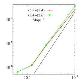
(a) $\|\mathbf{u}-{\bf w}\|_{{\bf L}^{2}}$ versus $\tau$

(b) $\|p-q\|_{L^{2}}$ versus $\tau$

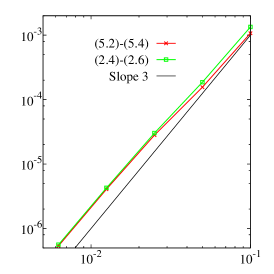
(c) $\|\nabla\!{\cdot}{\bf w}\|_{L^{2}}$ versus $\tau$

Figure 1. Log-log plot of the ${\bf L}^{2}$-norm of the error at $T=10$ of the 2D unsteady Stokes equations on a $200\times 200$ MAC grid. Continuous lines represent the slope 3, solid lines with $\times$ symbols represent the results with (5.2)-(5.4), solid lines with $\Box$ symbols represent the results with (2.4)-(2.6).

Next, we compare the accuracy of the second order scheme (5.2)-(5.3) and the second order direction-splitting bootstrapping scheme (5.5)-(5.6) in figure 2. Although being slightly less accurate in the pressure, the direction splitting scheme clearly has a good potential since it is less computationally demanding; we recall that this schemes only requires the solution of tridiagonal problems and thus can be massively parallelized as in Guermond and Minev [3].

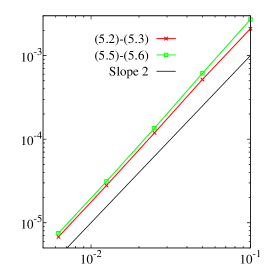
(a) $\|\mathbf{u}-{\bf w}\|_{{\bf L}^{2}}$ versus $\tau$

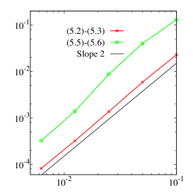
(b) $\|p-q\|_{L^{2}}$ versus $\tau$

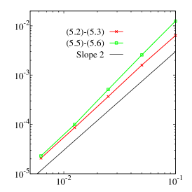
(c) $\|\nabla\!{\cdot}{\bf w}\|_{L^{2}}$ versus $\tau$

Figure 2. Log-log plot of the ${\bf L}^{2}$-norm of the error at $T=10$ of the 2D unsteady Stokes equations on a $200\times 200$ MAC grid. Continuous lines represent the slope 2, solid lines with $\times$ symbols represent the results with (5.2)-(5.3), solid lines with $\Box$ symbols represent the results with (5.5)-(5.6).

Finally we present 3D numerical results that demonstrate the accuracy of (5.2)-(5.3) in the case of the unsteady Stokes and the Navier-Stokes problem at Re=100. The 3D manufactured solution is given by: $u_{1}=\cos x\sin y\sin(z+t),u_{2}=\sin x\cos y\sin(z+t),u_{3}=-2\sin x\sin y\cos(z+t),p=\cos(x+y+z+t)$. The results on a grid of $20\times 20\times 20$ MAC cells are presented in figure 3. Again, the defect correction method (5.2)-(5.3) demonstrates good accuracy and robustness, maintaing stability even at relatively large time steps $dt=0.1$.

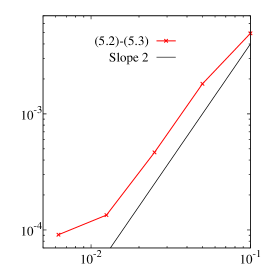
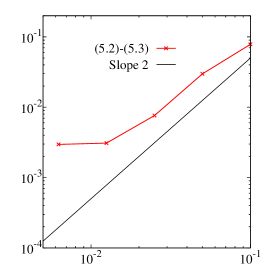
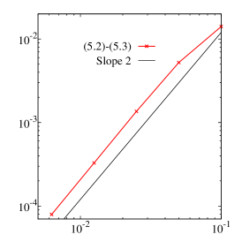
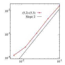
(a) $\|\mathbf{u}-{\bf w}\|_{{\bf L}^{2}}$ versus $\tau$

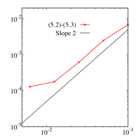
(b) $\|p-q\|_{L^{2}}$ versus $\tau$

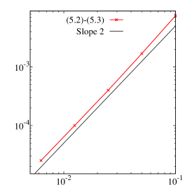
(c) $\|\nabla\!{\cdot}{\bf w}\|_{L^{2}}$ versus $\tau$

Figure 3. Log-log plot of the ${\bf L}^{2}$-norm of the error at $T=10$ on a $20\times 20\times 20$ MAC grid. Top row: 3D unsteady Stokes equations, bottom row: 3D Navier-Stokes equations at Re=100. Continuous lines represent the slope of 2, solid lines with $\times$ symbols represent the results with (5.2)-(5.3).

7. Conclusions

In this paper we have revisited the high-order artificial compressibility methods for incompressible flow of Guermond and Minev [2] and we have demonstrated that the coupling of the Cartesian components of the velocity, which is due to the presence of the implicit $\nabla\nabla\!{\cdot}$ operator, can be avoided. The resulting schemes thus require only the solution of a set of classical scalar parabolic problems of the type: $u_{k}-\tau\nabla\!{\cdot}\left(\kappa\nabla u_{k}\right)=f$. These schemes can also be factorized direction-wise to yield computationally very simple, and yet accurate direction splitting schemes.

When compared to the classical Chorin-Temam-type projection schemes, the algorithms proposed in this paper are computationally more efficient since they require the solution of problems with conditioning scaling like $\tau h^{-2}$ whereas projection methods require the solution of an elliptic problem for the pressure whose conditioning scales like $h^{-2}$. In addition, the present approach allows to develop schemes of any order in time unlike the projection methods whose accuracy is limited to second order.

References

- Douglas [1962] J. Douglas, Jr. Alternating direction methods for three space variables. Numer. Math., 4:41–63, 1962.
- Guermond and Minev [2015] J.-L. Guermond and P. Minev. High-order time stepping for the incompressible Navier-Stokes equations. SIAM J. Sci. Comput., 37(6):A2656–A2681, 2015.
- Guermond and Minev [2011] J.-L. Guermond and P. D. Minev. A new class of massively parallel direction splitting for the incompressible Navier-Stokes equations. Computer Methods in Applied Mechanics and Engineering, 200(23-24):2083–2093, 2011.
- Ladyzhenskaya [1970] O. A. Ladyzhenskaya. The mathematical theory of viscous incompressible flow (in Russian). Second Russian Edition, revised and extended. Nauka, Moscow, 1970.
- Temam [1977] R. Temam. Navier–Stokes Equations, volume 2 of Studies in Mathematics and its Applications. North-Holland, 1977.
- Vabishchevich [2014] P. Vabishchevich. Additive operator-difference schemes: splitting schemes. De Gruyter, Berlin, Boston, 2014.
- Vladimirova et al. [1966] N. Vladimirova, B. Kuznetsov, and N. Yanenko. Numerical calculation of the symmetrical flow of viscous incompressible liquid around a plate (in Russian). In Some Problems in Computational and Applied Mathematics. Nauka, Novosibirsk, 1966.
- Yanenko [1971] N. N. Yanenko. The method of fractional steps. The solution of problems of mathematical physics in several variables. Springer-Verlag, New York, 1971.