HectoMAP and Horizon Run 4: Dense Structures and Voids in the Real and Simulated Universe

Abstract

HectoMAP is a dense redshift survey of red galaxies covering a 53 deg² strip of the northern sky. HectoMAP is 97% complete for galaxies with $r<20.5$, $(g-r)>1.0$, and $(r-i)>0.5$. The survey enables tests of the physical properties of large-scale structure at intermediate redshift against cosmological models. We use the Horizon Run 4, one of the densest and largest cosmological simulations based on the standard $\Lambda$ Cold Dark Matter ($\Lambda$CDM) model, to compare the physical properties of observed large-scale structures with simulated ones in a volume-limited sample covering 8$\times 10^{6}$ $h^{-3}$ Mpc³ in the redshift range $0.22<z<0.44$. We apply the same criteria to the observations and simulations to identify over- and under-dense large-scale features of the galaxy distribution. The richness and size distributions of observed over-dense structures agree well with the simulated ones. Observations and simulations also agree for the volume and size distributions of under-dense structures, voids. The properties of the largest over-dense structure and the largest void in HectoMAP are well within the distributions for the largest structures drawn from 300 Horizon Run 4 mock surveys. Overall the size, richness and volume distributions of observed large-scale structures in the redshift range $0.22<z<0.44$ are remarkably consistent with predictions of the standard $\Lambda$CDM model.

1. INTRODUCTION

Galaxy redshift surveys are a powerful tool of modern cosmology. The large-scale three-dimensional distribution of galaxies on scales ranging from a few Mpc to a few hundreds Mpc contains important information about the initial fluctuations that shape structure in the universe. The physical properties of the observed large-scale structure including size, richness and density distributions are useful probes of the physics of structure formation, and they contribute to the determination of cosmological parameters including the matter density and dark energy (e.g., Tegmark et al. 2004; Eisenstein et al. 2005). Recent analysis of large-scale galaxy clustering in combination with other observations including the cosmic microwave background and Type Ia Supernovae suggests that we live in a universe consistent with the $\Lambda$ Cold Dark Matter ($\Lambda$CDM) model, a homogeneous, isotropic universe with Gaussian primordial fluctuations dominated by dark energy and with the matter density of $\sim 30\%$ (see Weinberg et al. 2013 for references).

The largest structures in the local universe revealed by galaxy redshift surveys (e.g., the CfA Great Wall by Geller & Huchra 1989) are an additional test of the standard paradigm (Park, 1990). As the volume covered by redshift surveys has increased, larger structures were identified including the Sloan Great Wall at $z\sim 0.08$ and extending for $\sim$320 $h^{-1}$ Mpc (Gott et al., 2005). The existence of these large structures, especially if there are even larger structures, might be a challenge to current models of structure formation (Springel et al., 2006; Sheth & Diaferio, 2011; Park et al., 2012, 2015).

Cosmic voids, vast low density space in the universe, are also an important probe of structure formation models (Kim & Park, 1998; Sheth & van de Weygaert, 2004; Park et al., 2012; Cai et al., 2015). Identification of voids and comparison of their properties with simulations is a large-scale measure of the galaxy distribution that is less sensitive than dense structures to complex baryonic physics. The statistics of the physical properties of voids (e.g., distributions of size, shape, or volume) can provide useful constraints on the cosmological parameters (Sutter et al., 2012a; Jennings et al., 2013), modified gravity models (Clampitt et al., 2013), and dark energy models (Bos et al., 2012; Pisani et al., 2015). However, identification of voids and their measured properties are sensitive to the survey parameters, particularly the sampling density (Sutter et al., 2014a). When the sampling density of surveys is lower, small voids disappear; the remaining voids become larger and more spherical, and tend to have slightly steeper radial density profiles (Sutter et al., 2014a). These issues can have an important impact on the comparison with cosmological models.

Several numerical simulations follow void evolution in the context of hierarchical structure formation (Colberg et al., 2005; Padilla et al., 2005). However, there are few observational studies of void evolution as a result of the lack of dense redshift surveys beyond the local universe. Conroy et al. (2005) used the Deep Extragalactic Evolutionary Probe 2 (DEEP2, Davis et al. 2005) redshift survey to show that the voids at $z\sim 0.1$ are larger than those at $z\sim 1$, approximately as expected. Micheletti et al. (2014) have identified voids at $0.55<z<0.9$ in the VIMOS Public Extragalactic Redshift Survey (VIPERS; Guzzo et al. 2014), but complex selection effects prevent detailed study of size evolution of these voids (see also Sutter et al. 2014b for the voids at $z=0.43-0.7$ from the Sloan Digital Sky Survey (SDSS; York et al. 2000)). As Sutter et al. (2014a) emphasize the importance of sampling density in characterizing the physical properties of voids, a redshift survey that is both dense enough and extensive enough to study the evolution of voids and over-dense structures is necessary for exploring the properties of these structures at a range of cosmic epochs.

Here we use a new survey, HectoMAP, to investigate the characteristics of large-scale dense structures and voids. HectoMAP covers a 52.97 deg² region of the sky (Geller et al., 2011; Geller & Hwang, 2015). HectoMAP is a dense redshift survey of red galaxies designed to explore large-scale structure in the redshift range $0.2<z<0.7$. The ultimate limiting magnitude of the survey will be $r=21.3$. We focus the 97% complete sample with a limiting $r=20.5$. For the redshift range it covers, HectoMAP currently offers a unique combination of high sampling density ($\sim 600$ galaxies deg^-2 for the galaxies at $r<20.5$) and large volume ($3.1\times 10^{7}$ $h^{-3}$ Mpc³). Eventual completion of the HectoMAP survey to $r=21.3$ will nearly double the sampling density on the sky to $\sim 1200$ galaxies deg^-2.

HectoMAP complements the Baryon Oscillation Spectroscopic Survey (BOSS; Dawson et al. 2013), a similar color-selected redshift survey, covering a much larger volume for the galaxies at $z<0.7$ ($5.4\times 10^{9}$ $h^{-3}$ Mpc³ in a 9376 deg² region). BOSS is designed to measure the scale of baryon acoustic oscillations (BAO; Eisenstein et al. 2001; Dawson et al. 2013). Many studies have reported impressive detections of the baryon oscillation scale based on the BOSS data (e.g. Kazin et al. 2010; Percival et al. 2010; Padmanabhan et al. 2012).

The sampling in the BOSS survey is significantly sparser than HectoMAP. BOSS includes redshifts of 1.5 million luminous galaxies at $i\leq 19.9$ over 10,000 deg^-2 (i.e. $\sim 150$ galaxies per square degrees). The denser sampling of the HectoMAP survey allows study of the individual rich clusters, voids and the surrounding large-scale structures.

Over the next few years the HectoMAP regions will be surveyed with Hyper Suprime-Cam (HSC, Miyazaki et al. 2012) on Subaru. The resulting weak lensing map will complement the redshift survey in mapping the dark matter distribution. In a pilot survey (Kurtz et al., 2012), we demonstrate that HectoMAP matches the sensitivity of the expected Subaru weak-lensing maps. The comparison of weak-lensing peaks with system identified in redshift surveys is an important test of the issues limiting applications to the measurement of cluster masses and to the application of weak lensing cluster counts as a cosmological tool (Geller et al., 2010, 2014a; Van Waerbeke et al., 2013; Hwang et al., 2014).

Here we use HectoMAP to delineate large-scale features in a volume-limited subsample of the survey covering the redshift range $0.22<z<0.44$. We compare the results with structures identified in exactly the same way from the Horizon Run 4 cosmological $N$-body simulations (Kim et al., 2015). We compare distributions of the characteristics of dense structures and voids. We also investigate the properties of the largest dense structure and the largest void in both the real universe and the simulations.

The Horizon Run 4 is one of the densest and largest simulations; there are 6300³ particles in a cubic box of $L_{\rm box}=3150$ $h^{-1}$ Mpc with a minimum subhalo mass of 2.7$\times$10¹¹ $h^{-1}$ M_⊙ (30 dark matter particles). The simulations are large enough to provide 300 independent mock surveys for comparison with the data. The Horizon Run 4 simulations are dark matter only, but the comparison with galaxy distribution on large scales ($\gtrsim 10$ Mpc) is insensitive to baryonic physics (Kazin et al., 2010; van Daalen et al., 2011, 2014).

We describe the HectoMAP observations in Section 2 and the Horizon Run 4 simulations in Section 3. We explain the method and the sample where we identify large-scale structure in HectoMAP in Section 4. We apply the same procedure we use for the HectoMAP data to the Horizon Run 4 data in Section 5. Statistical comparisons between the observations and simulations are in Section 6. We compare the largest structures in HectoMAP and Horizon Run 4 in Section 7. We discuss the results and conclude in Sections 8 and 9, respectively. Throughout, we adopt flat $\Lambda$CDM cosmological parameters: $H_{0}=100$ $h$ km s^-1 Mpc^-1, $\Omega_{\Lambda}=0.74$, and $\Omega_{m}=0.26$ (WMAP 5-year data, Dunkley et al. 2009). All quoted errors in measured quantities are 1$\sigma$.

2. HectoMAP OBSERVATIONS

HectoMAP is a redshift survey of red galaxies, covering a 52.97 deg² strip of the sky with 200$\arcdeg\leq$ R.A.(J2000) $\leq$ 250$\arcdeg$ and 42.5$\arcdeg\leq$ Decl.(J2000) $\leq$ 44.0$\arcdeg$. Geller et al. (2011) and Geller & Hwang (2015) preview the survey and describe its initial goals. The ultimate goal of the survey is completion to $r=21.3$. Here we analyze the complete brighter portion of the survey for galaxies with $r<20.5$.

2.1. Photometry

We used SDSS DR7 photometry (DR7, Abazajian et al. 2009) to select targets for spectroscopic observations in 2010. Since 2013 we have used the updated DR9 photometric catalog (Ahn et al., 2012). Targets are red galaxies with $r_{\rm Petro,0}<21.3$, $(g-r)_{\rm fiber,0}>1.0$, $(r-i)_{\rm fiber,0}>0.5$, and $r_{\rm fiber,0}<22.0$. We examined a somewhat broader color selection in a pilot survey ($g-r>1.0$, $r-i>0.4$ and $r_{\rm Petro}<21.3$; Kurtz et al. 2012) where we compared apparent clusters in the redshift survey with weak-lensing peaks. Red galaxies satisfying the color selection we used are certainly a robust basis for cluster identification (see also Geller & Hwang 2015 for detailed discussion on the color selection criteria). In general, red galaxies are more clustered and the contrast of the large-scale structure is greater than blue galaxies (e.g., Madgwick et al. 2003; Park et al. 2007; Zehavi et al. 2011). The color selection efficiently rejects nearby galaxies at $z\leq 0.2$ where the overlap with the SDSS is substantial and where the lensing sensitivity drops steeply (see Geller et al. 2010).

Table 1HectoMAP Redshift Survey Properties

Parameter	Value
Survey Area (deg2)	52.97
Nphot,20.5,mag	32808
Nz,20.5,mag	31721
$z_{\rm med,20.5,mag}$	0.34
Nz,20.5,vol	9881

2.2. Spectroscopy

We obtained galaxy spectra with the Hectospec on the MMT 6.5m telescope (Fabricant et al., 1998, 2005). The Hectospec is a robotic instrument with 300 fibers deployable over 1$\arcdeg$ field of view. We used the 270 line mm^-1 grating of Hectospec that provides a dispersion of 1.2 $\AA$ pixel^-1 and a resolution of $\sim$6 $\AA$. Typical exposures were 0.75$-$1.5 hours. The resulting spectra cover the wavelength range 3650$-$9150 $\AA$.

We chose the HectoMAP strip at high declination (i.e. 42.5$\arcdeg\leq$ Decl. $\leq$ 44.0$\arcdeg$) so that it is always 30$\arcdeg$ away from the moon. Thus we can observe target galaxies in gray or even in bright time. The advantage of this high declination location is particularly favorable for the brighter portion of the survey we consider here.

To obtain a high, uniform spectroscopic completeness within the survey region down to the ultimate limiting magnitude of $r_{\rm Petro,0}=21.3$, we weighted the spectroscopic targets with their apparent magnitudes within the color range. We used the Hectospec observation planning software (Roll et al., 1998) to assign the fibers efficiently. We filled unused fibers with targets bluer than the color limits.

We reduced the Hectospec spectra obtained before 2013 with the Mink et al. (2007) pipeline. Beginning in 2014, we used HSRED v2.0, an updated reduction pipeline originally developed by Richard Cool. There is no systematic offset between redshifts derived from the two pipelines. We determined the redshifts by using RVSAO (Kurtz & Mink, 1998) to cross-correlate the spectra with templates. We visually inspected all of the spectra, and assigned a quality flag to the spectral fits with “Q” for high-quality redshifts, “?” for marginal cases, and “X” for poor fits. We use only the spectra with “Q” redshifts. Repeat observations of 1651 separate absorption-line and 238 separate emission-line objects provide mean internal errors normalized by $(1+z)$ of 48 and 24 km s^-1, respectively (Geller et al., 2014b).

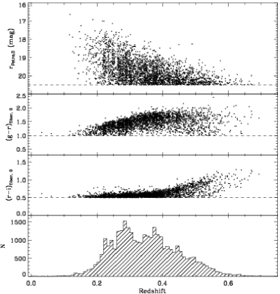
Figure 1.— (Top) $r$-band magnitudes, (Middle) ($g-r$) and ($r-i$) colors as a function of redshift for HectoMAP galaxies with $(g-r)_{\rm fiber,0}>1.0$, $(r-i)_{\rm fiber,0}>0.5$, $r_{\rm fiber,0}<22.0$, and $r_{\rm Petro,0}<20.5$. The horizontal line in each panel indicates these selection criteria. All magnitudes are Galactic-extinction corrected. We display only 10% of the data for clarity. (Bottom) Redshift distribution for HectoMAP.

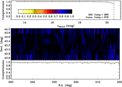
Figure 2.— Spectroscopic completeness for the sample of galaxies with $r_{\rm Petro,0}<20.5$ as a function of $r$-band magnitude (Top) and of right ascension (Bottom). Vertical line in the top panel is the magnitude limit, $r_{\rm Petro,0}=20.5$. (Middle) Two-dimensional spectroscopic completeness as a function of right ascension and of declination.

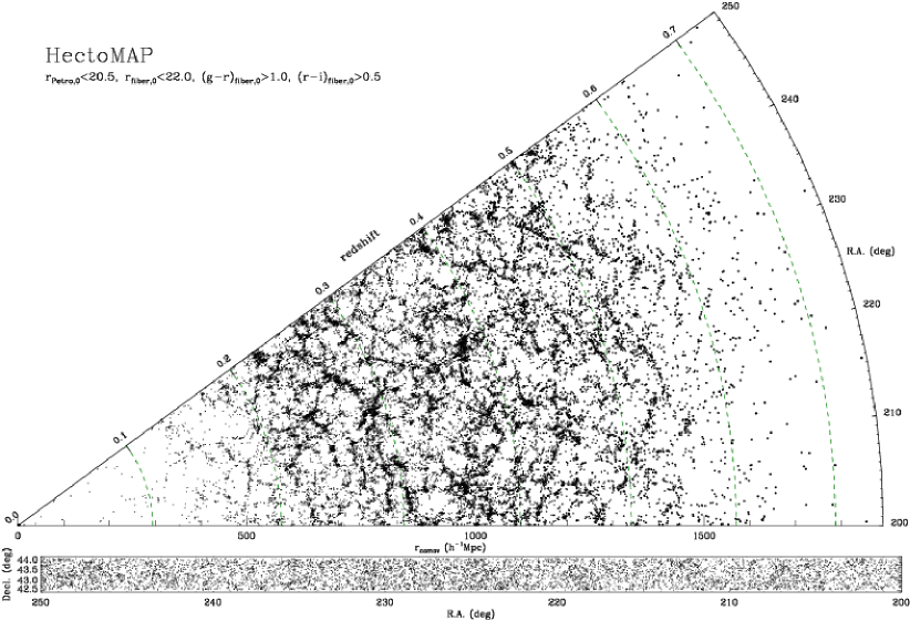
Figure 3.— (Top) Cone diagram for HectoMAP galaxies with $r_{\rm Petro,0}<20.5$. (Bottom) Distribution on the sky as a function of right ascension and declination. We display all the data in the top panel, but only 30% of the data for clarity in the bottom panel.

We observed the HectoMAP region in queue mode beginning in 2010. We expect to complete the survey to the deeper limiting magnitude $r=21.3$ in Spring 2016. We supplement the data with redshifts from the SDSS DR12 (Alam et al., 2015) and the NASA/IPAC Extragalactic Database (NED) including the literature (Gronwall et al., 2004; Jaffé et al., 2013). HectoMAP is now 97% complete to $r=20.5$ and includes 31721 redshifts. Among them, 30555 were acquired with Hectospec, 1165 were measured by the SDSS DR12 (Alam et al., 2015), and one was from Gronwall et al. (2004). Table 1 lists the number of galaxies in the photometric sample with $r_{\rm Petro,0}<20.5$ and the number of measured redshifts in the sample.

Figure 1 shows the HectoMAP color selection. Beginning from the top panel, we display, sequentially, the distributions of $r$-band apparent magnitudes, $(g-r)_{\rm fiber,0}$ and $(r-i)_{\rm fiber,0}$ colors. We plot only the galaxies satisfying the color selection. The histogram clearly demonstrates that the color selection efficiently rejects nearby galaxies with $z<0.2$. The median redshift of the red galaxy sample is $z\sim 0.34$.

The upper panel of Figure 2 shows the spectroscopic completeness for the sample with $(g-r)_{\rm fiber,0}>1.0$, $(r-i)_{\rm fiber,0}>0.5$, $r_{\rm fiber,0}<22.0$ and $r_{\rm Petro,0}<20.5$ as a function of apparent magnitude. The completeness curve is nearly flat and decreases only slightly at $r_{\rm Petro,0}>20$. The cumulative spectroscopic completeness for $r_{\rm Petro,0}<20.5$ is 97% with a differential completeness of 89% at $r_{\rm Petro,0}=20.5$. The middle panel shows a two-dimensional map of the completeness at $r_{\rm Petro,0}<20.5$ as a function of R.A. and decl. The two-dimensional map shows 200$\times$6 pixels for the survey region of 200$\arcdeg\leq$ R.A.(J2000) $\leq$ 250$\arcdeg$ and 42.5$\arcdeg\leq$ Decl.(J2000) $\leq$ 44.0$\arcdeg$. The map shows that the survey is highly complete over the survey region; there are only 37 pixels (3.1%) with completeness less than 85%. The bottom panel shows the integrated completeness as a function of R.A.

Figure 3 shows a cone diagram for the sample with $r_{\rm Petro,0}<20.5$ projected along the declination direction. The diagram shows the characteristic features of large-scale structure at intermediate redshift; fingers corresponding to clusters are obvious at $z<0.55$, and there are many voids delimited by thin walls and filaments. At $z>0.45$, the structures are less sharply defined than those at lower redshift because we have only very luminous galaxies at this redshift range (see Figure 4) and because the physical size of the survey slice is thicker at higher redshift than for lower redshift; the 1.5 degree slice corresponds to 25.7 and 12.6 $h^{-1}$ Mpc at $z=0.6$ and $z=0.2$, respectively.

3. HORIZON RUN 4 $N$-BODY SIMULATION

We use the Horizon Run 4 $N$-body simulation (Kim et al., 2015) as a foundation for comparing the large-scale features of HectoMAP with the predictions of structure formation models. This dark matter only simulation is one of the densest and largest available. It is large enough to contain many independent mock HectoMAP surveys and is thus ideal for the comparison.

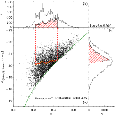
Figure 4.— $K$-corrected (to $z=0.4$) $r$-band absolute magnitudes for galaxies in HectoMAP as a function of redshift. The green curve indicates the apparent magnitude limit, $r_{\rm Petro,0}=20.5$. The orange solid line defines the lower limit for the galaxy sample that has a constant galaxy number density over the redshift range $0.22<z<0.44$ ($n_{\rm gal}=1.36\times 10^{-3}$ $h^{3}$ Mpc^-3 or $d_{\rm mean}=9.01$ $h^{-1}$ Mpc). The slanted red dashed line is the best fit to the orange line (see the equation in the panel); it defines a volume-limited sample of galaxies delimited by the vertical dashed lines. We display only 20% of the data for clarity. The open and red hatched histograms in top and right panels show the distributions of galaxies in the entire and volume-limited samples, respectively.

The Horizon Run is a series of cosmological $N$-body simulation run by Kim et al. (2011). Horizon Run 4 is the densest of these simulations with 6300³ particles in a cubic box of $L_{\rm box}=3150$ $h^{-1}$ Mpc. The simulation adopts a standard $\Lambda$CDM cosmology in accord with the WMAP 5-year data (Dunkley et al., 2009). The particle mass is $m_{p}\sim 9\times 10^{9}$ $h^{-1}$ M_⊙. The subhalos are identified with the physically self-bound (PSB) subhalo finding method (Kim & Park, 2006). The minimum mass of subhalos with 30 member particles is 2.7$\times$10¹¹ $h^{-1}$ M_⊙.

Horizon Run 4 provides past lightcone data up to $z\sim 1.5$. The true lightcones are important for comparison with a deep redshift survey like HectoMAP. Using simulated light cone data in redshift space, we first construct 300 non-overlapping mock surveys. Each mock survey has the same survey geometry as HectoMAP.

When we compare HectoMAP with Horizon Run 4, we assume that each dark matter subhalo contains only one galaxy. This subhalo-galaxy one-to-one correspondence assumption has worked successfully in many applications including the one-point function and its local density distribution (Kim et al., 2008), the two-point function (Kim et al., 2009; Nuza et al., 2013), the topology of galaxy distribution (Gott et al., 2009; Choi et al., 2010; Parihar et al., 2014), estimates of large-scale velocity moments (Agarwal et al., 2012), and identification of the largest structures (Park et al., 2012). We also match the halo number density of the mock data with the galaxy number density in HectoMAP (i.e. abundance matching, Kravtsov et al. 2004; Vale & Ostriker 2004; Conroy et al. 2006; Kim et al. 2008; Guo et al. 2010).

To test the sensitivity of structure identification to the method of matching the simulated halos to the HectoMAP galaxies, we construct two types of volume-limited samples of halos based on two different sampling methods. In the first method, we match the halo number density with the galaxy number density by assuming that more massive halos correspond to more luminous galaxies (Kravtsov et al., 2004; Vale & Ostriker, 2004; Conroy et al., 2006; Kim et al., 2008; Guo et al., 2010). A second approach mimics the known observational selection effects that exist in a red-selected sample like HectoMAP. Red galaxies are generally in denser regions (e.g., Blanton et al. 2005; Cooper et al. 2006; Park et al. 2007), and the more massive they are, the denser the surroundings (e.g., Lemson & Kauffmann 1999; Park et al. 2007; Haas et al. 2012). Obviously we do not have color information for halos in the simulation. Thus, we use the local density around red galaxies as a proxy for color. We measure the local density around galaxies in HectoMAP and match it to the local density distribution around halos in the simulation.

4. ANALYSIS OF HectoMAP

We construct a volume-limited sample of HectoMAP galaxies in Section 4.1 for robust comparison with the $N$-body simulations. We then identify over-dense large-scale features in Section 4.2 and under-dense structures in Section 4.3.

4.1. A Volume-Limited Sample of HectoMAP

To identify large-scale structures in HectoMAP for robust comparison with the $N$-body simulations, we first construct a volume-limited sample of galaxies with constant comoving number density. This approach is similar to the construction of the sample of luminous red galaxies for the study of large-scale structure in SDSS/BOSS (e.g., Eisenstein et al. 2001; Dawson et al. 2013). This procedure is the foundation for a fair comparison with the simulations based on the same comoving number density of halos (i.e. $1.36\times 10^{-3}$ $h^{3}$ Mpc^-3 or mean halo separation of 9.01 $h^{-1}$ Mpc), and for unbiased identification of large-scale structures within the redshift range of the sample.

To construct a volume-limited sample, we first plot the $r$-band absolute magnitudes for the $r_{\rm Petro,0}<20.5$ sample as a function of redshift (Figure 4). We use the Kcorrect software (ver. 4.2) of Blanton & Roweis (2007) for $K$-corrections. We then compute galaxy number densities by changing the lower limit in absolute magnitude as a function of redshift. The orange contour indicates the magnitude limit that yields a comoving number density of $1.36\times 10^{-3}$ $h^{3}$ Mpc^-3 at each redshift. To remove the effect of small-scale fluctuations, we fit the contour with a linear relation (slanted red dashed line). The vertical red dashed lines show the lower and upper redshift limits defining the volume-limited sample we analyze. The upper redshift limit of $z=0.44$ is set by the $r_{\rm Petro,0}=20.5$ (green solid line) magnitude limit of the redshift survey; the lower redshift limit is set by the ($r-i$) selection that eliminates low redshift objects.

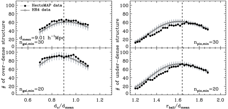
Figure 5.— (Top left) Number of over-dense structures with more than 30 member galaxies as a function of linking length in units of galaxy mean separation for HectoMAP (filled circles) and Horizon Run 4 (open circles). The error bars indicate the standard deviation in the number of structures derived from the 300 mock samples of Horizon Run 4. The vertical lines indicate the critical linking length we adopt (i.e. $d_{c}=0.9d_{\rm mean}$). (Bottom left) Same as top left panel, but for over-dense structures with more than 20 members. (Top right) Number of under-dense structures with more than 30 connected pixels as a function of the ball radius for HectoMAP (filled circles) and Horizon Run 4 (open circles). The vertical lines indicate the critical ball radius we adopt (i.e. $r_{\rm ball}=1.64d_{\rm mean}$). (Bottom right) Same as top right panel, but for under-dense structures with more than 20 connected pixels.

4.2. Identification of Over-dense Large-Scale Structures

We identify over- and under-dense large-scale structures using the method in Park et al. (2012). This method is similar to the application of a friends-of-friends algorithm (Aikio & Mähönen, 1998; Berlind et al., 2006) for identifying galaxy groups/clusters and cosmic voids. We explain the details in this section.

We apply a friends-of-friends algorithm (Huchra & Geller, 1982) to the volume-limited sample of HectoMAP galaxies to identify over-dense large-scale structures by connecting galaxies with a fixed linking length. To reduce the fingers along the line of sight resulting from peculiar motions in galaxy systems, we adopt a method similar to the ones used for SDSS galaxies in Tegmark et al. (2004) and Park et al. (2012). We first run the friends-of-friends algorithm with a short linking length of 3 $h^{-1}$ Mpc comparable with the diameter of a rich cluster. We then compare the dispersion of the linked structures along the line of sight with the dispersion in projected separation perpendicular to the line of sight. If the dispersion along the line of sight exceeds the perpendicular spread, we adjust the radial velocities of the member galaxies to have the same effective velocity dispersion in the two directions.

We again apply the friends-of-friends algorithm to the data after the correction for extension along the line-of-sight. This time we explore several linking lengths to identify the optimal linking length that gives the maximum number of structures (Basilakos, 2003). The left panels of Figure 5 show the number of over-dense structures identified as a function of linking length. The upper and lower panels show the numbers of structures containing more than 30 and 20 member galaxies, respectively (see filled circles for the HectoMAP data). The number of over-dense structures first increases with linking length and then decreases for a large enough linking length. We choose the length $d_{c}=0.9d_{\rm mean}=8.11$ $h^{-1}$ Mpc that gives the maximum number of structures as the critical linking length, and set 20 as the minimum number of member galaxies defining an over-dense structure. We explore different linking lengths further in Section 6.

The top panel of Figure 6 shows a cone diagram for the volume-limited sample of galaxies at $0.22<z<0.44$ (black dots). We mark the members of over-dense structures identified with the critical linking length of $d_{c}=0.9d_{\rm mean}$ with colored symbols. Many structures we identify are filamentary.

The richest and largest structure in this diagram is at R.A.$=$205.5 (deg), Decl.$=$43.2 (deg) and $z=0.36$; the maximum extent is 181.1 $h^{-1}$ Mpc with 443 members. The maximum extent is the maximum separation of member galaxies in a structure. We compute this extent in real space after reducing the extension of fingers in redshift space. For comparison, Park et al. (2012) derive a length of $\sim$150 $h^{-1}$ Mpc for the Sloan Great Wall using the SDSS galaxies. However, the linking length used in Park et al. is not the same as the one we use here. They used a sample of SDSS galaxies with $M_{r}\leq-21.6$, $z<0.17$, and $d_{\rm mean}=9$ $h^{-1}$ Mpc with a linking length of $0.622d_{\rm mean}$ ($=5.6$ $h^{-1}$ Mpc). If we use a linking length of $0.622d_{\rm mean}$, the largest structure in HectoMAP has a maximum extent of only 60.3 $h^{-1}$ Mpc with 135 members. Thus the extent of the apparently largest structure is a sensitive function of the linking length. Although the difference between HectoMAP and SDSS may result partly from differences in survey geometry (HectoMAP is essentially a 2D thin-slice survey whereas the SDSS is 3D), this comparison underscores the necessity of using identical procedures when comparing different redshift surveys or when comparing the data with a simulation.

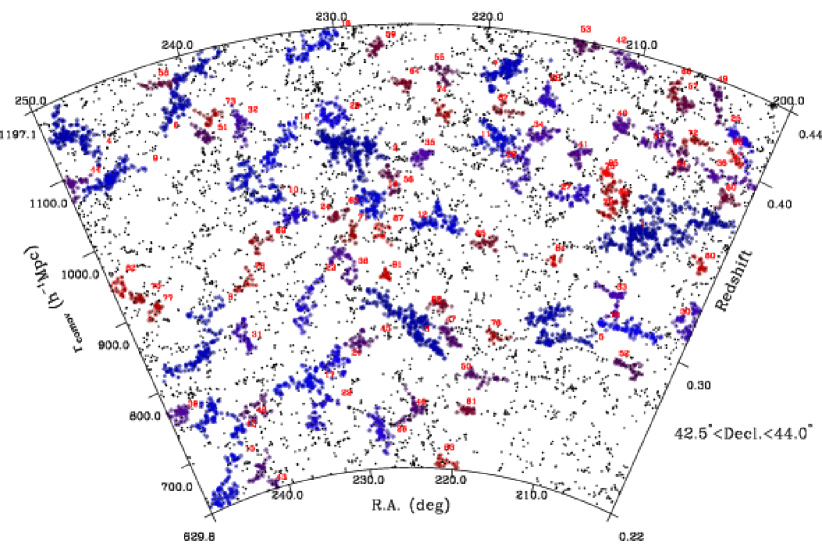
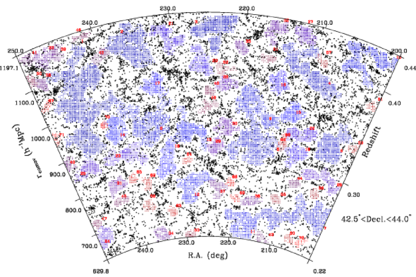
Figure 6.— (Top) Distribution of galaxies in the volume-limited sample derived from HectoMAP. The colored circles with numbers indicate over-dense structures identified with the friends-of-friends algorithm. (Bottom) Same as top panel, but for under-dense structures.

4.3. Identification of Voids: Under-Dense Structures

We also identify under-dense large-scale features or voids in HectoMAP. We begin by tessellating the three-dimensional survey region with cubic 4 $h^{-1}$ Mpc pixels ; we then count the number of galaxies within a radius of $r_{\rm ball}$ centered on each pixel. When we find $\leq 1$ galaxy within $r_{\rm ball}$, the pixel is a void pixel. We next connect the void pixels using a friends-of-friends algorithm to identify connected under-dense regions. We expand the void only to a distance of $r_{\rm ball}-d_{c}$ to account for a buffer region neighboring the over-dense structures (Park et al., 2012). The length $d_{c}$ is linking length we use to identify over-dense structures.

The right panels of Figure 5 show the number of under-dense structures we identify as a function of the ball radius, $r_{\rm ball}$. The upper and lower panels show the numbers of structures with more than 30 and 20 connected void pixels, respectively (see filled circles for the HectoMAP data). Similar to the over-dense case, the number of under-dense structures generally first increases with ball radius, but decreases when the ball radius is large enough. The change in the number of under-dense structures appears more sensitive to the change in effective linking length than the number of over-dense structures (left panel). We choose a ball radius of $r_{\rm ball}=1.64d_{\rm mean}=$ 14.78 $h^{-1}$ Mpc as the critical ball radius and a minimum of 20 pixels; this radius yields the maximal number of under-dense regions. We examine the impact of different ball radii in Section 6.

The bottom panel of Figure 6 highlights the under-dense structures with colored symbols. Many of the voids are elongated with complex morphologies. The largest under-dense region in both size and volume is at R.A.$=$244.0 (deg), Decl.$=$43.3 (deg) and $z=0.37$; with a maximum extent of 300.8 $h^{-1}$ Mpc and a volume of $3.80\times 10^{5}$ $h^{-3}$ Mpc³. The maximum extent of voids is the maximum separation of the void pixels in the structure. We compute this separation in real space. The largest SDSS void complex in Park et al. (2012) has a volume of $1.44\times 10^{6}$ $h^{-3}$ Mpc³ with a maximum extent of 334 $h^{-1}$ Mpc, apparently larger than the one in HectoMAP. However, the ball radius used in Park et al. is 1.45 $d_{\rm mean}$ ($=$13.06 $h^{-1}$ Mpc) for the sample of SDSS galaxies with $M_{r}\leq-21.6$, $z<0.17$, and $d_{\rm mean}=9$ $h^{-1}$ Mpc. If we use the same ball radius as in Park et al. (i.e. $1.45d_{\rm mean}$), the largest void in HectoMAP has a maximum extent of 883.6 $h^{-1}$ Mpc with a volume of $2.01\times 10^{6}$ $h^{-3}$ Mpc³, larger than the largest void in the SDSS (Park et al. 2012, see also Pan et al. 2012; Sutter et al. 2012b for size distribution of SDSS voids). As for the dense structures, differences between HectoMAP and SDSS may result partly from differences in survey geometry, but this exercise again emphasizes the necessity of using identical procedures when comparing physical properties of large-scale structure in different redshift surveys or when comparing the data with a simulation.

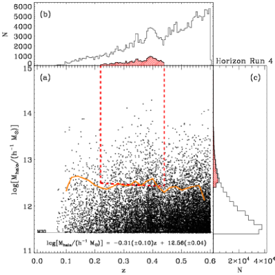
Figure 7.— Halo masses as a function of redshift in one mock sample from the Horizon Run 4 simulation. The orange solid line is the lower limit for the halo sample that provides a constant halo number density over the redshift range $0.1<z<0.57$ ($n_{\rm halo}=1.36\times 10^{-3}$ $h^{3}$ Mpc^-3 or $d_{\rm mean}=9.01$ $h^{-1}$ Mpc). The slanted red dashed line is the best fit to the orange line, and defines a volume-limited sample of halos delimited by the vertical dashed lines. The horizontal solid line indicates a minimum subhalo mass of 2.7$\times$10¹¹ $h^{-1}$ M_⊙ with 30 dark matter particles. We display only 5% of the data for clarity. The open and red hatched histograms in top and right panels show the distributions of halos in the entire and volume-limited samples, respectively.

5. ANALYSIS OF HORIZON RUN 4

Here we identify large-scale structures in the Horizon Run 4 simulation data using the same procedure we use for the observations. Sections 5.1 and 5.2 describe two methods of sampling the halos from the mock surveys.

5.1. Large-Scale Structures in Horizon Run 4: Sampling Based on Halo Mass

Figure 7 shows the distribution of halo masses as a function of redshift for one Horizon Run 4 mock survey. As for the HectoMAP data (Figure 4), we first determine the lower mass limit that gives a constant comoving number density of $1.36\times 10^{-3}$ $h^{3}$ Mpc^-3 at each redshift (orange solid line). We then derive the best-fit linear approximation to the contour (slanted red dashed line). The red dashed lines define the volume-limited sample of halos we use for a statistical comparison with the HectoMAP data. The limiting redshifts are the same as for HectoMAP.

To take the effect of our small spectroscopic incompleteness into account in the simulated data, we compute the spectroscopic completeness at each redshift and absolute magnitude in Figure 4 based on the completeness curve as a function of apparent magnitude (i.e. top panel of Figure 2). Because the galaxy number density at each redshift and absolute magnitude in Figure 4 corresponds to the halo number density at each redshift and halo mass in Figure 7, we remove halos in the appropriate bins of the simulations to match the data. By considering the spectroscopic completeness at each redshift and halo mass in Figure 7, we ensure that the number and distribution of halos we select from the simulations match number of observed galaxies in the volume-limited sample (i.e. 9881 galaxies).

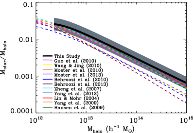
Figure 8.— Stellar-to-halo mass ratio as a function of halo mass for the volume-limited samples of HectoMAP galaxies and Horizon Run 4 subhalos. The black solid line is the best-fit relation in the halo mass range $2.3\times 10^{12}-9.9\times 10^{14}$ $h^{-1}$ $M_{\odot}$. The gray shaded region indicates the 1$\sigma$ dispersion of the distribution of galaxies and halos around the best-fit relation. For comparison, we show (colored dashed lines) relations from other studies with different methods: abundance matching (Guo et al., 2010; Wang & Jing, 2010; Moster et al., 2010, 2013; Behroozi et al., 2010, 2013), the halo occupation distribution (Zheng et al., 2007), the conditional luminosity function (Yang et al., 2012), and cluster catalogs (Lin & Mohr, 2004; Yang et al., 2009; Hansen et al., 2009). See Behroozi et al. (2013) for a more complete list of the relation with a detailed discussion.

To show the relationship between the subhalos in Horizon Run 4 and the galaxies in HectoMAP, we plot the stellar-to-halo mass ratio as a function of halo mass in Figure 8 for the volume-limited samples. We compute stellar masses using the SDSS five-band photometric data with the Le Phare code (Arnouts et al., 1999; Ilbert et al., 2006). Details of the stellar mass estimates are in Zahid et al. (2014). Because we use $r$-band absolute magnitudes to define the HectoMAP volume-limited sample (see Figure 4), we first sort the galaxies according to their $r$-band absolute magnitudes. We then sort the subhalos by mass (see Figure 7), and associate them with the galaxies in HectoMAP sample according to their rank. We combine all the subhalo-galaxy association from the 300 mock surveys, and fit to the data with the functional form in Moster et al. (2010, 2013),

$$\frac{M_{\rm star}}{M_{\rm halo}}=2N{\left[{\left(M_{\rm halo}/M_{1}\right)}^{-\beta}+{\left(M_{\rm halo}/M_{1}\right)}^{\gamma}\right]}^{-1}.$$ (1)

Because we cannot provide a good constraint on the slope at a small mass range (i.e. $M_{\rm halo}<10^{12}$ M_⊙), we fix $\beta=1$ (Moster et al., 2010, 2013). The best-fit parameters for the halo mass range $2.3\times 10^{12}-9.9\times 10^{14}$ $h^{-1}$ M_⊙ are $N=0.026$, $M_{1}=1.38\times 10^{12}$ $h^{-1}$ M_⊙, and $\gamma=0.664$. We plot the best-fit relation in Figure 8 as a black solid line; the stellar-to-halo mass ratio decreases with increasing subhalo mass. The gray shaded region indicates the 1$\sigma$ dispersion of the distribution of the data around the best-fit relation. For comparison, we show the relations (colored dashed lines) from other studies with different methods: abundance matching (e.g., Guo et al. 2010), the halo occupation distribution (e.g., Zheng et al. 2007), the conditional luminosity function (e.g., Yang et al. 2012), and cluster catalogs (e.g., Lin & Mohr 2004). This comparison substantiates our approach; our relation is consistent with a range of previous studies. There are several effects that may contribute to the large scatter among the relations (e.g., different simulation resolution, large uncertainty in stellar mass estimates, different galaxy samples, or different halo identification methods), but a detailed discussion is beyond the scope of this paper (see Behroozi et al. 2013 for a more complete list of the relation with a detailed discussion).

We now apply the friends-of-friends algorithm to the volume-limited samples of halos from the 300 mock surveys to identify over-dense large-scale structure. We also reduce fingers as in the HectoMAP data. The left panels of Figure 5 (open circles) show the number of over-dense structures from 300 mock surveys as a function of linking length (mean at each linking length). The overall behavior is similar to the one for the HectoMAP data. Using the same critical linking length as for the HectoMAP data, $d_{c}=0.9d_{\rm mean}$, we show the spatial distribution of structures marked by member halos in the top panel of Figure 9. The structures are similar to the over-dense structures in HectoMAP (Figure 6).

To identify under-dense features in the simulation, we again tessellate the three-dimensional survey region with cubic pixels, and count the number of halos within a radius of $r_{\rm ball}$ centered on each pixel. By connecting the void pixels with $\leq 1$ halo inside $r_{\rm ball}$, we obtain a list of under-dense regions.

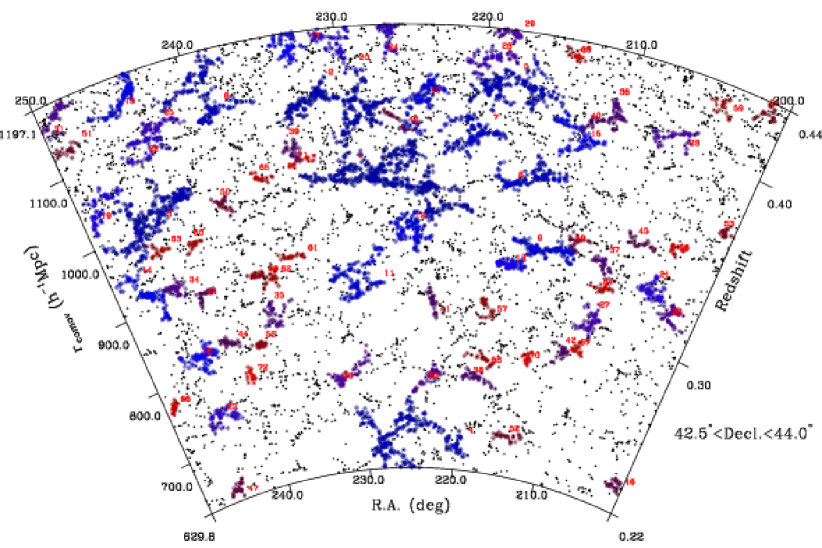
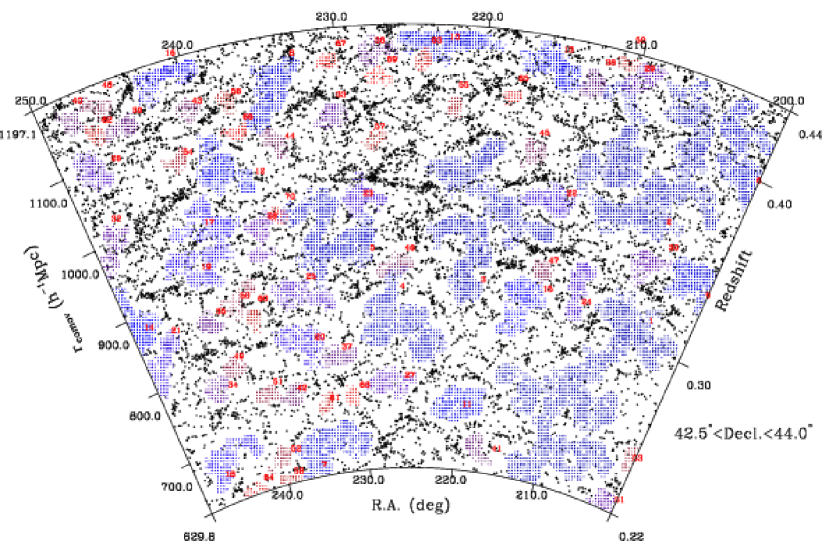
Figure 9.— Same as Figure 6, but for one of the mock surveys from Horizon Run 4.

The right panels of Figure 5 show the number of simulated under-dense structures (open circles) as a function of ball radius, $r_{\rm ball}$. Again, the numbers of under-dense regions in the simulation and observations behave similarly. We adopt the same ball radius of $r_{\rm ball}=1.64d_{\rm mean}$ as for HectoMAP because of the known sensitivity of the structures we identify to this scale (see the discussion of the comparison of the largest HectoMAP structures with the SDSS results at the end of Sections 4.2 and 4.3). The bottom panel of Figure 9 shows the Horizon Run 4 under-dense regions from one mock survey. Again, the morphologies are diverse and often complex. Section 6 contains a further discussion of the physical properties of these voids.

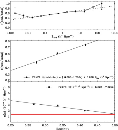
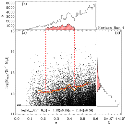
Figure 10.— (Bottom left) Galaxy number density in the combined data of F1 and F2 as a function of redshift using all the galaxies regardless of color (filled circles). The black solid line is the best-fit to the data. The red solid line indicates a constant number density of galaxies satisfying the HectoMAP color selection. (Top left) Fraction of HectoMAP selected galaxies as a function of surface galaxy number density in the combined F1 and F2 data at $0.22<z<0.44$. The dashed line is the best fit to the data. (Middle left) Change in HectoMAP selected galaxy fraction as a function of redshift for the combined F1 and F2 data (filled circles). The black solid line is the best-fit to the data. (Right) Same as Figure 7, but for one mock survey from Horizon Run 4. Note that the sampling of halos here is based on local density; it differs from the halo sample in Figure 7. We display only 5% of the data for clarity.

5.2. Horizon Run 4 Large-Scale Structures: Sampling Halos Based on Local Density

5.2.1 Sampling Halos

When we construct a volume-limited sample of halos in Section 5.1, we match the number density of observed galaxies with that of halos by assuming that more luminous massive halos correspond to more luminous galaxies without considering the HectoMAP red selection in detail. Although this approach is acceptable because the red galaxies are generally good tracers of matter distribution (e.g., Madgwick et al. 2003; Park et al. 2007; Zehavi et al. 2011; Kurtz et al. 2012), here we use local densities around halos to mimic the HectoMAP red selection. To evaluate the density distribution around the observed galaxies in HectoMAP, we use the SHELS (Smithsonian Hectospec Lensing Survey) survey. SHELS covers two separate 4 square degree fields of the Deep Lens Survey (F1 and F2) (Wittman et al., 2002, 2006). Currently SHELS is the densest redshift survey to its limiting apparent magnitude, $R=20.6$ (or $r\sim 20.9$). Unlike HectoMAP, SHELS is a complete magnitude-limited survey (Geller et al., 2005, 2010, 2014b, 2015). In other words, there is no color selection. Thus it can be used as a base for examining the HectoMAP color selection (Geller & Hwang, 2015).

We use the complete magnitude-limited survey, SHELS, to compute the fraction of red galaxies satisfying the HectoMAP selection as a function of surrounding local density and redshift. We then apply the relation we determine from SHELS to the simulation to select the fraction of halos that mimics the fraction of red galaxies with a given surrounding local density and redshift.

The steps in our construction of a sample of halos matching the red selection of HectoMAP are:

1. Using SHELS, we first construct a volume-limited sample of galaxies with $0.22<z<0.44$, similar to the sample in HectoMAP. We define the absolute magnitude limit as a function of redshift so that the number density of galaxies satisfying the HectoMAP color selection is constant with redshift as in HectoMAP (i.e. $d_{\rm mean}=9.01$ $h^{-1}$ Mpc). Because the fraction of HectoMAP selected galaxies changes with redshift, the number density of all the galaxies regardless of color in this volume-limited sample changes with redshift; the bottom left panel in Figure 10 shows this change.

2. Next we compute the surface galaxy number density around each galaxy using all the galaxies regardless of color with relative velocities $\Delta v\leq 1000$ km s^-1. We compute $\Sigma_{3}=3(\pi D^{2}_{p,3})^{-1}$ where $D_{p,3}$ is the projected distance to the 3rd-nearest neighbor galaxy. The typical physical scale of this $\Sigma_{3}$ probes is $2-3$ $h^{-1}$ Mpc, and our results do not change even if we use 5th-nearest neighbor galaxy.

3. We compute the fraction of HectoMAP selected galaxies as a function of $\Sigma_{3}$ in three redshift bins ($0.22<z<0.3$, $0.3<z<0.37$, and $0.37<z<0.44$), and determine the best-fit relation between this fraction and $\Sigma_{3}$ at each redshift: f(red/total)$=a+b\Sigma_{3}$. Figure 10 (upper left panel) shows an example of this fit at $0.22<z<0.44$.

4. We combine the best-fit relations in the three redshift bins to determine a global relation among the red galaxy fraction, redshift and local density: f(red/total)$=a_{0}+a_{1}z+b\Sigma_{3}$ where $a_{0}=0.003\pm 0.058$, $a_{1}=1.768\pm 0.158$ and $b=0.098\pm 0.013$ are the coefficients derived for the best-fit relation. Figure 10 (middle left panel) shows the redshift dependence of this relation when $b=0$ as an example.

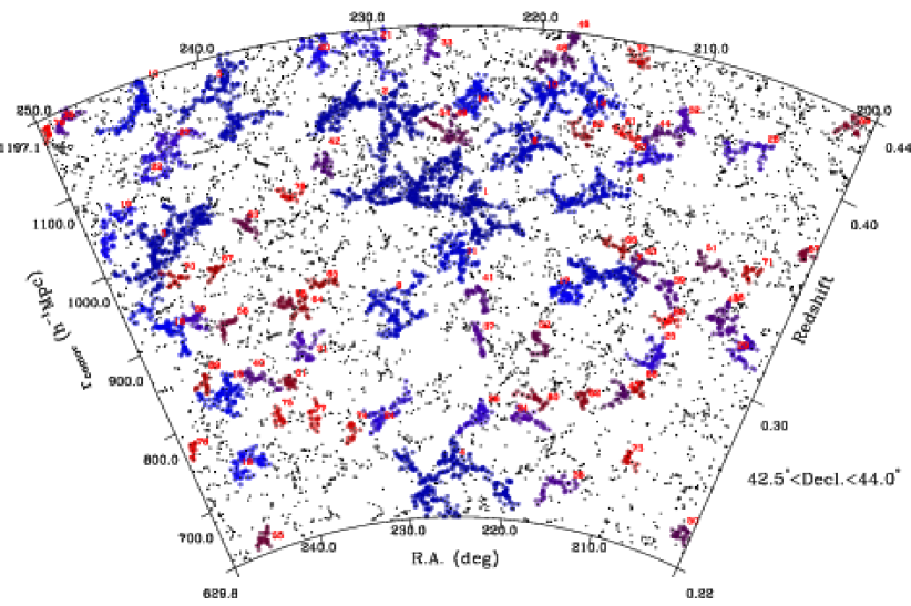
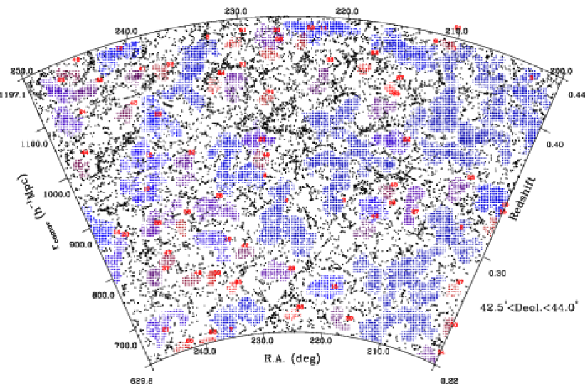
Figure 11.— Same as Figure 6, but for one of the mock surveys from Horizon Run 4. The sampling of halos here is based on local density; it differs from the halo sample in Figure 9.

For a galaxy sample following the relation, f(red/total)$=0.003+1.768z+0.098\Sigma_{3}$, the number density of red galaxies is independent of redshift as in the volume-limited sample of HectoMAP galaxies. We thus apply this relation to the Horizon Run 4 mock surveys next.

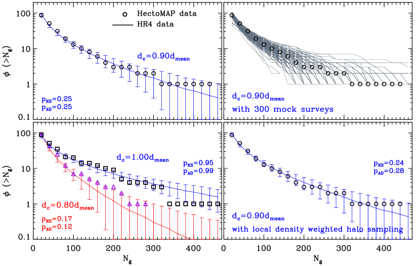
Figure 12.— (Top left) Cumulative richness distribution of over-dense large-scale structures identified with the critical linking length of $d_{c}=0.9d_{\rm mean}$ (HectoMAP: open circles, Horizon Run 4: blue solid lines). The error bars indicate the standard deviation in the richness distributions from the 300 mock surveys of Horizon Run 4. Two numbers in the left corner indicate $p$-values from the K-S and A-D k-sample tests on the distributions of the HectoMAP and Horizon Run 4 data. The sampling of halos is based on halo mass (see Section 5.1). The gray curve in the top right panel indicates the distribution for each mock survey, and the open circles are the same as in the left panel. (Bottom left) Same as top left panel, but for the distributions with two different linking lengths ($d_{c}=1.0d_{\rm mean}$: squares and blue solid line, $d_{c}=0.8d_{\rm mean}$: triangles and red solid line). (Bottom right) Same as top left panel, but for the distribution from different mock surveys of the Horizon Run 4, based on local density weighted halo sampling (see Section 5.2).

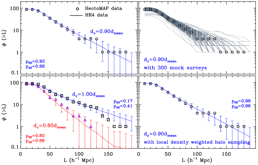
Figure 13.— Same as Figure 12, but for the cumulative size distribution of over-dense large-scale structures.

1. In the plot of halo mass and redshift for a mock survey, we determine the lower mass limit that follows the change of galaxy number density with redshift determined at (1.1); the orange line in the right panel of Figure 10 shows this limit. The best-fit relation to the orange line (slant red dashed line) defines the volume-limited sample of halos at $0.22<z<0.44$.

2. With the volume-limited sample of halos defined at (2.1), we compute the surface number density around each halo using the 3rd-nearest neighbor halo: $\Sigma_{3}=3(\pi D^{2}_{p,3})^{-1}$.

3. We select a fraction of halos at each redshift and local density from the mock survey that matches the fraction of HectoMAP selected galaxies determined from the relation among the HectoMAP selected galaxy fraction, redshift and local density at (1.4). We keep the total number of selected halos in a mock survey the same as the total number of HectoMAP galaxies in the volume-limited sample at $0.22<z<0.44$ (i.e. $N=9881$).

5.2.2 Horizon Run 4 Large-Scale Structure with Local Density Selection

We again apply the friends-of-friends algorithm to the 300 volume-limited samples of halos selected to mimic the observational selection. We identify over-dense large-scale structures. Figure 11 (upper panel) shows the spatial distribution of structures marked by these halos in one mock sample based with a linking length of $d_{c}=0.9d_{\rm mean}$. The bottom panel shows the distribution of under-dense regions using the void-finding algorithm of Section 4.3. Both the over-dense and under-dense structures in the simulations and observations are indistinguishable by eye. We compare the simulations and the observations quantitatively in the next section.

6. COMPARISON OF OBSERVED AND SIMULATED LARGE-SCALE STRUCTURES

Here we make a quantitative comparison between the over-dense and under-dense structures in HectoMAP and the Horizon Run 4 simulations. We first compare over-dense structures, and then under-dense structures. We use several measures to compare distributions of the properties of these structures. For the non-parametric measures, the Kolmogorov-Smirnov (K-S) test and the Anderson-Darling (A-D) k-sample test, we list the relevant $p$-value in each figure. The $p$-values indicate the probability that the data and the simulations are drawn from the same parent distribution.

The physical properties of the observed large-scale structures depend strongly on (or are restricted by) the survey geometry. The HectoMAP is a thin slice survey, covering a 53 deg² strip that is only 1.5 deg wide. Although the extent of a structure along the declination direction is essentially unconstrained by the data, there is no bias in our comparison between observations and simulations because the Horizon Run 4 mock surveys have the same geometry as HectoMAP.

6.1. Over-dense Large-Scale Structures

Figure 12 (upper left) shows the cumulative richness distribution of over-dense structures in HectoMAP (open circles) and in the Horizon Run 4 simulation (blue solid curve). More precisely, the cumulative distribution is the number of structures per survey volume ($7.89\times 10^{6}$ $h^{-3}$ Mpc³) that include $\geq n_{g}$ member galaxies. The critical linking length is $d_{c}=0.9d_{\rm mean}$. The error bar indicates the dispersion in the richness distribution based on the 300 mock surveys. The plot shows that the richness distributions of over-dense structures in both the observations and simulations data agree within the 1$\sigma$ error bars.

To highlight the richness distribution from the 300 mock surveys, we show the distribution for each mock survey with a gray curve in the top right panel. The distribution of the observations (open circles) lies well within the range of the distributions for the 300 mock surveys.

To examine the sensitivity of our results to the linking length, we show the richness distributions for the observations and simulations based on two different linking lengths (bottom left panel). The differences between the observations and simulations, particularly for the $d_{c}=0.8d_{\rm mean}$, appear to be slightly larger than for $d_{c}=0.9d_{\rm mean}$ but the observations still agree with the simulations within the error bars.

The bottom right panel shows the analogous richness distribution for the simulation data based on local density sampling and $d_{c}=0.9d_{\rm mean}$ (see Section 5.2). The correspondence between the observations and the simulations is excellent.

In all panels of Figure 12, the K-S and A-D $p$-values reject the null hypothesis at the $\lesssim 1.5\sigma$ level. This weak rejection is consistent with the comparison of the data and simulations based on the error bars.

Figure 13 shows the cumulative size distribution of over-dense structures (i.e. number of structures with maximum extent larger than $L$). As in the previous plots, the top left panel shows the distributions of structures in the HectoMAP (open circles) and Horizon Run 4 data (blue solid curve) based on the critical linking length of $d_{c}=0.9d_{\rm mean}$. The two distributions agree well.

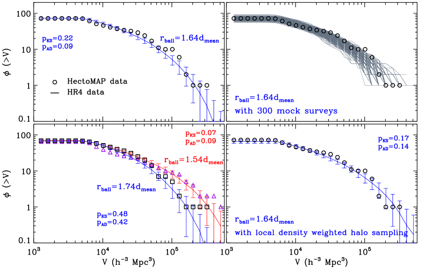
Figure 14.— (Top left) Cumulative volume distribution of under-dense large-scale structures identified with the critical ball radius of $r_{\rm ball}=1.64d_{\rm mean}$ (HectoMAP: open circles, Horizon Run 4: blue solid lines). The error bars indicate the standard deviation in the size distributions from the 300 mock surveys of Horizon Run 4. Two numbers in the left corner indicate $p$-values from the K-S and A-D k-sample tests on the distributions of the HectoMAP and Horizon Run 4 data. The sampling of halos is based on halo mass (see Section 5.1). The gray curve in the top right panel indicates the distribution from each mock survey, and the open circles are the same as in the top left panel. (Bottom left) Same as top left panel, but for distributions with two different ball radii ($r_{\rm ball}=1.74d_{\rm mean}$: squares and blue solid line, $r_{\rm ball}=1.54d_{\rm mean}$: triangles and red solid line). (Bottom right) Same as top left panel, but for the distribution from different mock surveys of the Horizon Run 4, based on local density weighted halo sampling (see Section 5.2).

The top right panel compares the distribution from the observations (open circles) with the 300 mock surveys (gray curves). The bottom left panel shows the result of using different linking lengths (i.e. $d_{c}=0.8d_{\rm mean}$ and $1.0d_{\rm mean}$). The bottom right panel shows the impact of sampling the simulation based on local density sampling of halos (see Section 5.2). All panels show that the observed and simulated universes are remarkably similar. The K-S and A-D $p$-values reject the null hypothesis for these distributions at an even weaker level than for the distributions in Figure 12. Because the match between the two is excellent, the dispersion in the 300 mock surveys can give us a robust measure of the probable error in the physical properties of observed large-scale structures.

6.2. Voids: Under-dense Structure

Here we compare the volume and size distributions of under-dense large-scale structures (voids) in HectoMAP and the Horizon Run 4 simulation. Figure 14 (top left panel) shows the cumulative volume distribution of under-dense structures in HectoMAP (open circles) and in the Horizon Run 4 simulation (blue solid curve). The cumulative distribution tracks the number of structures with volume $>V$. We use a critical ball radius, $r_{\rm ball}=1.64d_{\rm mean}$. The error bar indicates the dispersion among the 300 mock surveys. The two distributions agree well even though there is a small offset between the two around $V\sim 10^{5}$ ($h^{-3}$ Mpc³). The distributions from the individual 300 mock surveys (gray curves in the top right panel) suggest that the small offset is statistically insignificant; The planned deeper HectoMAP survey with $r_{\rm Petro,0}<21.3$ will roughly double the galaxy number density. With this denser sample, we will be able to study any systematic issue that might be responsible for this small difference.

The bottom left panel shows the volume distribution of under-dense structures based on two different ball radii ($r_{\rm ball}=1.74d_{\rm mean}$: squares and blue solid line, $r_{\rm ball}=1.54d_{\rm mean}$: triangles and red solid line). The distributions of observations and simulations agree well within the error bars. The bottom right panel shows a similar volume distribution with $r_{\rm ball}=1.64d_{\rm mean}$, but for simulated halos based on local density sampling (see Section 5.2). The correspondence between the observations and simulations appears better than the case based on halo mass sampling (top left panel).

In the panels of Figure 14, the K-S and A-D $p$-values reject the null hypothesis at a significance $\lesssim 1.8\sigma$. This weak rejection is again consistent with the correspondence between observations and simulations based on the error bars.

Figure 15 shows the cumulative size distribution of under-dense structures (i.e. number of structures with maximum extent $>L$). The top left panel shows the agreement between the distribution of HectoMAP (open circles) and Horizon Run 4 data (blue solid curve) based on a critical ball radius of $r_{\rm ball}=1.64d_{\rm mean}$.

The top right panel shows the distribution from the observations compared with the 300 mock surveys. The bottom left panel shows results for two different ball radii (i.e. $r_{\rm ball}=1.54d_{\rm mean}$ and $r_{\rm ball}=1.74d_{\rm mean}$). Here we see the only case where one of the statistical tests (the K-S test) rejects the null hypothesis at the $2\sigma$ level. Even this rejection, limited to only one of the two tests, is weak.

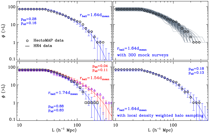
Figure 15.— Same as Figure 14, but for the cumulative size distribution of under-dense large-scale structures.

The bottom right panel shows the result for the simulations with halos selected on the basis of local density sampling (see Section 5.2). Here the K-S and A-D statistics reject the null hypothesis at the $\lesssim 1.5\sigma$ level. The correspondence between the observations and simulations is impressive in all of the comparisons we make.

7. THE LARGEST STRUCTURES IN HectoMAP and HORIZON RUN 4

The largest structures known in the universe, the CfA Great Wall (Geller & Huchra, 1989) and the Sloan Great Wall (Gott et al., 2005), led to interesting tests of models of structure formation. Several studies asked whether the existence of such structures is compatible with a universe that is homogeneous and isotropic on large scales (e.g., Clowes et al. 2012; Horvath et al. 2013). This issue has been tested and resolved several times through careful statistical comparison of the physical properties of large-scale structure in the observations and simulations, particularly in the nearby universe (Springel et al., 2006; Sheth & Diaferio, 2011; Park et al., 2012, 2015; Alpaslan et al., 2014). Here we revisit the issue by comparing the properties of the largest structures in HectoMAP with results from the 300 Horizon Run 4 mock surveys.

Figure 16 shows the distributions of the characteristics of over-dense structures and under-dense structures (voids) derived from the 300 Horizon Run 4 mock surveys. The left four panels show the results for sampling based on halo mass. The distributions are obviously not Gaussian; they have long tails stretching toward large values of the parameter. They resemble log-normal distributions as expected on theoretical grounds (Sheth & Diaferio, 2011). In each panel the arrow indicates the parameter for the largest structure in HectoMAP. We also indicate the fraction of mock surveys that contain a structure exceeding the scale for the observed structure. It is striking that the void parameters lie in the tails of the distribution whereas the dense structures lie relatively near the median for the mock surveys. This conclusion is consistent with the results of statistical comparisons between observations and simulations in Figures 12-15; the only $\sim$2$\sigma$ rejection of similarity between the observations and simulations occurs for under-dense structures with sampling based on halo mass (see bottom left panels in Figures 14 and 15).

Figure 16.— (Left) Distributions of the characteristics of the largest structures derived from the 300 Horizon Run 4 mock surveys. The halo sampling is based on halo mass. The top two panels show the richness and size distributions of over-dense structures. The bottom two panels show the volume and size distributions of under-dense structures. In each panel, the arrow indicates the parameter for the largest structure in HectoMAP. The number in each panel indicates the fraction of mock surveys that contain a structure exceeding the scale for the observed structure. (Right) Same as left panels, but for local density weighted sampling of simulated halos.

The right four panels of Figure 16 show the same distributions but for local density weighted sampling of simulated halos. For the largest over-dense structure, the relationship between the real universe and the mock surveys is clearly insensitive to the method of matching the mock surveys to the data. However, the lower two panels show that a comparison based on local density weighted halo sampling has a substantial effect on the parameters characterizing under-dense structures. Here the largest voids in HectoMAP are well within the range of the distribution for the mock surveys. In the results based on a match of halo mass to stellar mass, the parameters of the largest observed low density region are in the upper 10$-$16% of the simulated distribution: when the selection of simulated halos is weighted by local density to mimic the observational selection, the characteristics of the largest low density region are in the upper 31$-$33% of the simulated distribution. This result is similar to the results of Section 6.2 where the distribution of parameters characterizing the low density regions is more similar to local density weighted halo matching. For example, in Figure 14 (upper right) the cumulative distribution of void volumes for the data lies near the edge of the distribution for the mock surveys; in Figure 14 (lower right), the HectoMAP distribution is very close to the distribution for the mock surveys analyzed with local density weighted halo sampling.

Use of the largest structures as a test of the models is limited by the extended tails of the parameter distributions. The largest dense structure in the mock surveys (maximum extent: 560 $h^{-1}$ Mpc from mass weighted halo sampling) is essentially as large as it can be to still fit within the HectoMAP region. Although this structure is clearly an outlier in the simulated distribution, its mere presence is a warning about the robustness of apparent inconsistencies based on observations of a single large structure. With local density weighted halo sampling, the maximum extent of the largest structure is much smaller, 310 $h^{-1}$ Mpc.

Use of the largest structure as a robust test of the models would require observations of several well-separated (independent) volumes comparable with HectoMAP. As emphasized in Sections 4.2 and 4.3, comparisons of different surveys of the real universe and comparison between the models and the observations are sensitive to the details of the analysis method; the approach must be identical for clean comparisons.

8. DISCUSSION

The combination of HectoMAP and Horizon Run 4 enables extension of statistical comparisons between the real and simulated universe to regions at $z>0.2$. Surprisingly, the richness and size distributions of over-dense large-scale structures in HectoMAP agree impressively with the Horizon Run 4 simulations. The agreement also holds for under-dense structures or voids. Thus the standard $\Lambda$CDM model based on large-scale isotropy and homogeneity with Gaussian primordial fluctuations successfully accounts for the observed large-scale structure in the galaxy distribution up to $z=0.44$.

We note that the Horizon Run 4 simulations are dark matter only. Thus the remarkable agreement between the observed and simulated universes suggests that baryonic physics does not play a major role on the scales we explore. This conclusion is consistent with previous successful comparisons of the observed large-scale galaxy distribution with halo distribution of dark matter only simulations. The SDSS/BOSS red galaxy samples, for example, imply a similar conclusion (e.g., Sánchez et al. 2012; Manera et al. 2013; Nuza et al. 2013; Parihar et al. 2014). The dense sampling of HectoMAP and the huge volume covered by SDSS/BOSS are complementary tests of the consistency between the models and the data.

Compared to previous studies, there are several improvements in the comparison of the data with the simulations here. We examine the physical properties of both over- and under-dense large-scale structures at intermediate redshift (i.e. $0.22<z<0.44$) by combining the dense, wide-field redshift survey data (i.e. HectoMAP) with similarly dense, large simulation data (i.e. Horizon Run 4).

We use simulated true lightcones drawn from the Horizon Run 4 simulation. Most other comparisons are based on snapshots from the simulations. Because HectoMAP measures large-scale structure beyond the local universe, it is important to use true lightcones analogous to the observed universe (see Section 3.1 in Kim et al. 2015 for details on the construction of lightcone and snapshots for Horizon Run 4).

The volume of Horizon Run 4 is about 3300 times larger than the volume of HectoMAP at $0<z<0.44$. We thus can generate 300 non-overlapping HectoMAP-like mock surveys from the Horizon Run 4 simulation. These non-overlapping mock surveys from a huge simulation volume reinforce the statistical accuracy in the comparison between observations and simulations. Because the match between the observations and the simulations is excellent, the dispersion in the properties of the 300 simulations gives us a robust measure of the probable error in the HectoMAP assessment of the properties of large-scale structure. These 300 mock surveys enable exploration of the largest over-dense structure and the largest void for comparison with their HectoMAP counterparts. The observed structures are well within the range spanned by the mock surveys.

The physical properties of observed large-scale structures including richness, size and volume distributions strongly depend on the tracers and the method of identifying the tracers (Park et al., 2012, 2015). We thus emphasize the use of the same criteria in identifying large-scale structures in the observations and simulations (i.e. friends-of-friends algorithm with the same linking length and the void-finding algorithm with the same ball radius) using comparable volume-limited samples of galaxies and halos matched according to number densities averaged over large volumes. We also mimic the observational selection effects (i.e. the choice of red galaxies) in the simulations by matching the local density surrounding halos with those around the observed galaxies. These controls enable a fair, reliable comparison of the physical properties of large-scale structures in the real and simulated universe.

9. CONCLUSIONS

HectoMAP is a red-selected dense redshift survey, covering 53 deg² region of the sky to a limiting magnitude of $r_{\rm Petro,0}=20.5$. Its high sampling density and large volume provides a new basis for comparing large-scale structures in the real and simulated universe in the redshift range $0.22<z<0.44$, covering a volume of $7.89\times 10^{6}$ $h^{-3}$ Mpc³. We identify over- and under-dense large-scale structures in HectoMAP and in 300 non-overlapping matched mock surveys drawn from the Horizon Run 4 simulations. These observations and mock surveys provide a well-controlled comparison of over-dense and under-dense large scale features of the galaxy distribution beyond the local universe.

We identify over-dense large-scale structure in HectoMAP using the volume-limited sample of red galaxies with $0.22<z<0.44$. There are 87 over-dense structures with $N_{\rm member}\geq 20$ derived with a friends-of-friends algorithm and a linking length of $d_{c}=0.9d_{\rm mean}$ where $d_{\rm mean}$ is 9.01 $h^{-1}$ Mpc. The richest and largest structure is at $z=0.36$ with a maximum extent of 181.1 $h^{-1}$ Mpc and 443 member galaxies. We construct 300 non-overlapping mock surveys from the Horizon Run 4 cosmological $N$-body simulation with the same halo number density as in the HectoMAP volume-limited sample. We identify over-dense large-scale structures in these mock surveys using the same criteria as in HectoMAP. The richness and size distributions of the observed and simulated large-scale structures agree. The agreement is insensitive to reasonable changes in the linking length or in the method constructing volume-limited sample of halos to mimic the data.

We also identify under-dense large-scale structures using the same volume-limited samples of galaxies. There are 72 under-dense structures with $N_{\rm pixel}\geq 20$ in the sample based on a ball radius of $r_{\rm ball}=1.64d_{\rm mean}$. The largest structure is at $z=0.37$ with a maximum extent of 300.8 $h^{-1}$ Mpc and a volume of $3.8\times 10^{5}$ $h^{-3}$ Mpc³. We also identify under-dense structures in the 300 mock surveys using the same criteria as in HectoMAP. The volume and size distributions of observed and simulated voids are essentially identical and insensitive to reasonable changes in halo selection or in ball radius.

The size and richness (volume) distributions of observed over- and under-dense structures at $0.22<z<0.44$ in HectoMAP match those in the Horizon Run 4 dark matter only simulations. The largest structures seen in HectoMAP are well within the range of comparable structures identified in the 300 Horizon Run 4 mock surveys. Thus on large scales, the features of the galaxy distribution are insensitive to baryonic physics. The standard $\Lambda$CDM cosmological model accounts remarkably well for the structure we observe.

HectoMAP will eventually extend to $r_{\rm Petro,0}<21.3$. The surface number density of galaxies will roughly double ($\sim 1200$ per square degree). We then expect to identify large-scale structures to $z\sim 0.7$ thus enabling exploration of the evolution of large-scale structures. To set the stage for the evolutionary considerations it would be interesting to use the SDSS to construct local analogs to the HectoMAP sample that could be analyzed with essentially identical methods as a basis for the assessment of evolution from redshift zero to $z=0.7$.

Facility: MMT Hectospec

We thank the referee for a helpful and prompt report. The Smithsonian Institution supports the research of M.J.G., D.G.F., M.J.K., P.B., M.C., S.T., and S.M.. H.J.Z. is supported by the Clay Postdoctoral Fellowship. This work was supported by the Supercomputing Center/Korea Institute of Science and Technology Information with supercomputing resources including technical support (KSC-2013-G2-003). We thank Korea Institute for Advanced Study for providing computing resources (KIAS Center for Advanced Computation) for this work. Funding for SDSS-III has been provided by the Alfred P. Sloan Foundation, the Participating Institutions, the National Science Foundation, and the U.S. Department of Energy Office of Science. The SDSS-III web site is http://www.sdss3.org/. SDSS-III is managed by the Astrophysical Research Consortium for the Participating Institutions of the SDSS-III Collaboration including the University of Arizona, the Brazilian Participation Group, Brookhaven National Laboratory, Carnegie Mellon University, University of Florida, the French Participation Group, the German Participation Group, Harvard University, the Instituto de Astrofisica de Canarias, the Michigan State/Notre Dame/JINA Participation Group, Johns Hopkins University, Lawrence Berkeley National Laboratory, Max Planck Institute for Astrophysics, Max Planck Institute for Extraterrestrial Physics, New Mexico State University, New York University, Ohio State University, Pennsylvania State University, University of Portsmouth, Princeton University, the Spanish Participation Group, University of Tokyo, University of Utah, Vanderbilt University, University of Virginia, University of Washington, and Yale University. This research has made use of the NASA/IPAC Extragalactic Database (NED) which is operated by the Jet Propulsion Laboratory, California Institute of Technology, under contract with the National Aeronautics and Space Administration.

References

- Abazajian et al. (2009) Abazajian, K. N., Adelman-McCarthy, J. K., Agüeros, M. A., et al. 2009, ApJS, 182, 543
- Agarwal et al. (2012) Agarwal, S., Feldman, H. A., & Watkins, R. 2012, MNRAS, 424, 2667
- Ahn et al. (2012) Ahn, C. P., Alexandroff, R., Allende Prieto, C., et al. 2012, ApJS, 203, 21
- Aikio & Mähönen (1998) Aikio, J., & Mähönen, P. 1998, ApJ, 497, 534
- Alam et al. (2015) Alam, S., Albareti, F. D., Allende Prieto, C., et al. 2015, ApJS, 219, 12
- Alpaslan et al. (2014) Alpaslan, M., Robotham, A. S. G., Driver, S., et al. 2014, MNRAS, 438, 177
- Arnouts et al. (1999) Arnouts, S., Cristiani, S., Moscardini, L., et al. 1999, MNRAS, 310, 540
- Basilakos (2003) Basilakos, S. 2003, MNRAS, 344, 602
- Behroozi et al. (2010) Behroozi, P. S., Conroy, C., & Wechsler, R. H. 2010, ApJ, 717, 379
- Behroozi et al. (2013) Behroozi, P. S., Wechsler, R. H., & Conroy, C. 2013, ApJ, 770, 57
- Berlind et al. (2006) Berlind, A. A., Frieman, J., Weinberg, D. H., et al. 2006, ApJS, 167, 1
- Blanton et al. (2005) Blanton, M. R., Eisenstein, D., Hogg, D. W., Schlegel, D. J., & Brinkmann, J. 2005, ApJ, 629, 143
- Blanton & Roweis (2007) Blanton, M. R., & Roweis, S. 2007, AJ, 133, 734
- Bos et al. (2012) Bos, E. G. P., van de Weygaert, R., Dolag, K., & Pettorino, V. 2012, MNRAS, 426, 440
- Cai et al. (2015) Cai, Y.-C., Padilla, N., & Li, B. 2015, MNRAS, 451, 1036
- Choi et al. (2010) Choi, Y.-Y., Park, C., Kim, J., et al. 2010, ApJS, 190, 181
- Clampitt et al. (2013) Clampitt, J., Cai, Y.-C., & Li, B. 2013, MNRAS, 431, 749
- Clowes et al. (2012) Clowes, R. G., Campusano, L. E., Graham, M. J., & Söchting, I. K. 2012, MNRAS, 419, 556
- Colberg et al. (2005) Colberg, J. M., Sheth, R. K., Diaferio, A., Gao, L., & Yoshida, N. 2005, MNRAS, 360, 216
- Conroy et al. (2006) Conroy, C., Wechsler, R. H., & Kravtsov, A. V. 2006, ApJ, 647, 201
- Conroy et al. (2005) Conroy, C., Coil, A. L., White, M., et al. 2005, ApJ, 635, 990
- Cooper et al. (2006) Cooper, M. C., Newman, J. A., Croton, D. J., et al. 2006, MNRAS, 370, 198
- Davis et al. (2005) Davis, M., Gerke, B. F., Newman, J. A., & Deep2 Team. 2005, in Astronomical Society of the Pacific Conference Series, Vol. 339, Observing Dark Energy, ed. S. C. Wolff & T. R. Lauer, 128
- Dawson et al. (2013) Dawson, K. S., Schlegel, D. J., Ahn, C. P., et al. 2013, AJ, 145, 10
- Dunkley et al. (2009) Dunkley, J., Komatsu, E., Nolta, M. R., et al. 2009, ApJS, 180, 306
- Eisenstein et al. (2001) Eisenstein, D. J., Annis, J., Gunn, J. E., et al. 2001, AJ, 122, 2267
- Eisenstein et al. (2005) Eisenstein, D. J., Zehavi, I., Hogg, D. W., et al. 2005, ApJ, 633, 560
- Fabricant et al. (2005) Fabricant, D., Fata, R., Roll, J., et al. 2005, PASP, 117, 1411
- Fabricant et al. (1998) Fabricant, D. G., Hertz, E. N., Szentgyorgyi, A. H., et al. 1998, in Society of Photo-Optical Instrumentation Engineers (SPIE) Conference Series, Vol. 3355, Optical Astronomical Instrumentation, ed. S. D’Odorico, 285–296
- Geller et al. (2005) Geller, M. J., Dell’Antonio, I. P., Kurtz, M. J., et al. 2005, ApJ, 635, L125
- Geller et al. (2011) Geller, M. J., Diaferio, A., & Kurtz, M. J. 2011, AJ, 142, 133
- Geller & Huchra (1989) Geller, M. J., & Huchra, J. P. 1989, Science, 246, 897
- Geller & Hwang (2015) Geller, M. J., & Hwang, H. S. 2015, Astronomische Nachrichten, 336, 428
- Geller et al. (2015) Geller, M. J., Hwang, H. S., Dell’Antonio, I. P., et al. 2015, ApJS, submitted
- Geller et al. (2014a) Geller, M. J., Hwang, H. S., Diaferio, A., et al. 2014a, ApJ, 783, 52
- Geller et al. (2014b) Geller, M. J., Hwang, H. S., Fabricant, D. G., et al. 2014b, ApJS, 213, 35
- Geller et al. (2010) Geller, M. J., Kurtz, M. J., Dell’Antonio, I. P., Ramella, M., & Fabricant, D. G. 2010, ApJ, 709, 832
- Gott et al. (2009) Gott, J. R., Choi, Y.-Y., Park, C., & Kim, J. 2009, ApJ, 695, L45
- Gott et al. (2005) Gott, III, J. R., Jurić, M., Schlegel, D., et al. 2005, ApJ, 624, 463
- Gronwall et al. (2004) Gronwall, C., Salzer, J. J., Sarajedini, V. L., et al. 2004, AJ, 127, 1943
- Guo et al. (2010) Guo, Q., White, S., Li, C., & Boylan-Kolchin, M. 2010, MNRAS, 404, 1111
- Guzzo et al. (2014) Guzzo, L., Scodeggio, M., Garilli, B., et al. 2014, A&A, 566, A108
- Haas et al. (2012) Haas, M. R., Schaye, J., & Jeeson-Daniel, A. 2012, MNRAS, 419, 2133
- Hansen et al. (2009) Hansen, S. M., Sheldon, E. S., Wechsler, R. H., & Koester, B. P. 2009, ApJ, 699, 1333
- Horvath et al. (2013) Horvath, I., Hakkila, J., & Bagoly, Z. 2013, arXiv:1311.1104
- Huchra & Geller (1982) Huchra, J. P., & Geller, M. J. 1982, ApJ, 257, 423
- Hwang et al. (2014) Hwang, H. S., Geller, M. J., Diaferio, A., Rines, K. J., & Zahid, H. J. 2014, ApJ, 797, 106
- Ilbert et al. (2006) Ilbert, O., Arnouts, S., McCracken, H. J., et al. 2006, A&A, 457, 841
- Jaffé et al. (2013) Jaffé, Y. L., Poggianti, B. M., Verheijen, M. A. W., Deshev, B. Z., & van Gorkom, J. H. 2013, MNRAS, 431, 2111
- Jennings et al. (2013) Jennings, E., Li, Y., & Hu, W. 2013, MNRAS, 434, 2167
- Kazin et al. (2010) Kazin, E. A., Blanton, M. R., Scoccimarro, R., et al. 2010, ApJ, 710, 1444
- Kim & Park (2006) Kim, J., & Park, C. 2006, ApJ, 639, 600
- Kim et al. (2008) Kim, J., Park, C., & Choi, Y.-Y. 2008, ApJ, 683, 123
- Kim et al. (2009) Kim, J., Park, C., Gott, III, J. R., & Dubinski, J. 2009, ApJ, 701, 1547
- Kim et al. (2015) Kim, J., Park, C., L’Huillier, B., & Hong, S. E. 2015, Journal of Korean Astronomical Society, 48, 213
- Kim et al. (2011) Kim, J., Park, C., Rossi, G., Lee, S. M., & Gott, III, J. R. 2011, Journal of Korean Astronomical Society, 44, 217
- Kim & Park (1998) Kim, M., & Park, C. 1998, Journal of Korean Astronomical Society, 31, 109
- Kravtsov et al. (2004) Kravtsov, A. V., Berlind, A. A., Wechsler, R. H., et al. 2004, ApJ, 609, 35
- Kurtz et al. (2012) Kurtz, M. J., Geller, M. J., Utsumi, Y., et al. 2012, ApJ, 750, 168
- Kurtz & Mink (1998) Kurtz, M. J., & Mink, D. J. 1998, PASP, 110, 934
- Lemson & Kauffmann (1999) Lemson, G., & Kauffmann, G. 1999, MNRAS, 302, 111
- Lin & Mohr (2004) Lin, Y.-T., & Mohr, J. J. 2004, ApJ, 617, 879
- Madgwick et al. (2003) Madgwick, D. S., Hawkins, E., Lahav, O., et al. 2003, MNRAS, 344, 847
- Manera et al. (2013) Manera, M., Scoccimarro, R., Percival, W. J., et al. 2013, MNRAS, 428, 1036
- Micheletti et al. (2014) Micheletti, D., Iovino, A., Hawken, A. J., et al. 2014, A&A, 570, A106
- Mink et al. (2007) Mink, D. J., Wyatt, W. F., Caldwell, N., et al. 2007, in ASP Conf. Ser., Vol. 376, Astronomical Data Analysis Software and Systems XVI, ed. R. A. Shaw, F. Hill, & D. J. Bell, 249
- Miyazaki et al. (2012) Miyazaki, S., Komiyama, Y., Nakaya, H., et al. 2012, in Proc. SPIE, Vol. 8446, 0
- Moster et al. (2013) Moster, B. P., Naab, T., & White, S. D. M. 2013, MNRAS, 428, 3121
- Moster et al. (2010) Moster, B. P., Somerville, R. S., Maulbetsch, C., et al. 2010, ApJ, 710, 903
- Nuza et al. (2013) Nuza, S. E., Sánchez, A. G., Prada, F., et al. 2013, MNRAS, 432, 743
- Padilla et al. (2005) Padilla, N. D., Ceccarelli, L., & Lambas, D. G. 2005, MNRAS, 363, 977
- Padmanabhan et al. (2012) Padmanabhan, N., Xu, X., Eisenstein, D. J., et al. 2012, MNRAS, 427, 2132
- Pan et al. (2012) Pan, D. C., Vogeley, M. S., Hoyle, F., Choi, Y.-Y., & Park, C. 2012, MNRAS, 421, 926
- Parihar et al. (2014) Parihar, P., Vogeley, M. S., Gott, III, J. R., et al. 2014, ApJ, 796, 86
- Park (1990) Park, C. 1990, MNRAS, 242, 59P
- Park et al. (2007) Park, C., Choi, Y., Vogeley, M. S., Gott, J. R. I., & Blanton, M. R. 2007, ApJ, 658, 898
- Park et al. (2012) Park, C., Choi, Y.-Y., Kim, J., et al. 2012, ApJ, 759, L7
- Park et al. (2015) Park, C., Song, H., Einasto, M., Lietzen, H., & Heinamaki, P. 2015, Journal of Korean Astronomical Society, 48, 75
- Percival et al. (2010) Percival, W. J., Reid, B. A., Eisenstein, D. J., et al. 2010, MNRAS, 401, 2148
- Pisani et al. (2015) Pisani, A., Sutter, P. M., Hamaus, N., et al. 2015, Phys. Rev. D, 92, 083531
- Roll et al. (1998) Roll, J. B., Fabricant, D. G., & McLeod, B. A. 1998, in SPIE Conf. Ser., Vol. 3355, Optical Astronomical Instrumentation, ed. S. D’Odorico, 324–332
- Sánchez et al. (2012) Sánchez, A. G., Scóccola, C. G., Ross, A. J., et al. 2012, MNRAS, 425, 415
- Sheth & Diaferio (2011) Sheth, R. K., & Diaferio, A. 2011, MNRAS, 417, 2938
- Sheth & van de Weygaert (2004) Sheth, R. K., & van de Weygaert, R. 2004, MNRAS, 350, 517
- Springel et al. (2006) Springel, V., Frenk, C. S., & White, S. D. M. 2006, Nature, 440, 1137
- Sutter et al. (2014a) Sutter, P. M., Lavaux, G., Hamaus, N., et al. 2014a, MNRAS, 442, 462
- Sutter et al. (2012a) Sutter, P. M., Lavaux, G., Wandelt, B. D., & Weinberg, D. H. 2012a, ApJ, 761, 187
- Sutter et al. (2012b) —. 2012b, ApJ, 761, 44
- Sutter et al. (2014b) Sutter, P. M., Lavaux, G., Wandelt, B. D., et al. 2014b, MNRAS, 442, 3127
- Tegmark et al. (2004) Tegmark, M., Blanton, M. R., Strauss, M. A., et al. 2004, ApJ, 606, 702
- Vale & Ostriker (2004) Vale, A., & Ostriker, J. P. 2004, MNRAS, 353, 189
- van Daalen et al. (2011) van Daalen, M. P., Schaye, J., Booth, C. M., & Dalla Vecchia, C. 2011, MNRAS, 415, 3649
- van Daalen et al. (2014) van Daalen, M. P., Schaye, J., McCarthy, I. G., Booth, C. M., & Dalla Vecchia, C. 2014, MNRAS, 440, 2997
- Van Waerbeke et al. (2013) Van Waerbeke, L., Benjamin, J., Erben, T., et al. 2013, MNRAS, 433, 3373
- Wang & Jing (2010) Wang, L., & Jing, Y. P. 2010, MNRAS, 402, 1796
- Weinberg et al. (2013) Weinberg, D. H., Mortonson, M. J., Eisenstein, D. J., et al. 2013, Phys. Rep., 530, 87
- Wittman et al. (2006) Wittman, D., Dell’Antonio, I. P., Hughes, J. P., et al. 2006, ApJ, 643, 128
- Wittman et al. (2002) Wittman, D. M., Tyson, J. A., Dell’Antonio, I. P., et al. 2002, in SPIE Conf. Ser=., ed. J. A. Tyson & S. Wolff, Vol. 4836, 73–82
- Yang et al. (2009) Yang, X., Mo, H. J., & van den Bosch, F. C. 2009, ApJ, 695, 900
- Yang et al. (2012) Yang, X., Mo, H. J., van den Bosch, F. C., Zhang, Y., & Han, J. 2012, ApJ, 752, 41
- York et al. (2000) York, D. G., Adelman, J., Anderson, Jr., J. E., et al. 2000, AJ, 120, 1579
- Zahid et al. (2014) Zahid, J., Dima, G., Kudritzki, R., et al. 2014, ApJ, 791, 130
- Zehavi et al. (2011) Zehavi, I., Zheng, Z., Weinberg, D. H., et al. 2011, ApJ, 736, 59
- Zheng et al. (2007) Zheng, Z., Coil, A. L., & Zehavi, I. 2007, ApJ, 667, 760