GAP Safe Screening Rules for Sparse-Group Lasso

Abstract

In high dimensional settings, sparse structures are crucial for efficiency, either in term of memory, computation or performance. In some contexts, it is natural to handle more refined structures than pure sparsity, such as for instance group sparsity. Sparse-Group Lasso has recently been introduced in the context of linear regression to enforce sparsity both at the feature level and at the group level. We adapt to the case of Sparse-Group Lasso recent safe screening rules that discard early in the solver irrelevant features/groups. Such rules have led to important speed-ups for a wide range of iterative methods. Thanks to dual gap computations, we provide new safe screening rules for Sparse-Group Lasso and show significant gains in term of computing time for a coordinate descent implementation.

Keywords — Lasso, Group-Lasso, Sparse-Group Lasso, screening, safe rules, duality gap

1 Introduction

Sparsity is a critical property for the success of regression methods, especially in high dimension. Often, group (or block) sparsity is helpful when some known group structure needs to be enforced. This is for instance the case in multi-task learning (Argyriou et al., 2008) or multinomial logistic regression (Bühlmann & van de Geer, 2011, Chapter 3). In the multi-task setting, the group structure appears natural since one aims at jointly recovering signals whose supports are shared. In this context, sparsity and group sparsity are generally obtained by adding a regularization term to the data-fitting: $\ell_{1}$ norm for simple sparsity and $\ell_{1,2}$ for group sparsity.

Along with recent works on hierarchical regularization Jenatton et al. (2011); Sprechmann et al. (2011); Simon et al. (2013) have focused on a specific case: the Sparse-Group Lasso. This method is the solution of a (convex) optimization program with a regularization term that is a convex combination of the two aforementioned norms, enforcing sparsity and group sparsity at the same time.

When using such advanced regularizations, the computational burden can be heavy particularly in high dimension. Yet, it can be significantly reduced if one can exploit the fact that the solution of the optimization problem is sparse. Following the seminal paper on “safe screening rules” (El Ghaoui et al., 2012), many contributions have investigated such strategies (Xiang et al., 2011; Bonnefoy et al., 2014, 2015; Wang & Ye, 2014). These so called safe screening rules compute some tests on dual feasible points to eliminate primal variables whose coefficients are guaranteed to be zero in the exact solution. Still, the computation of a dual feasible point can be challenging when the regularization is more complex than $\ell_{1}$ or $\ell_{1,2}$ norms. This is the case for the Sparse-Group Lasso as it is not straightforward to characterize efficiently if a dual point is feasible or not (Wang & Ye, 2014). Hence, an efficient computation of the associated dual norm is required. This is all the more challenging that a naive implementation computing the dual norm associated to the Sparse-Group Lasso is very expensive (it is quadratic with respect to the groups dimensions).

Here, we propose efficient dynamic safe screening rules (i.e., rules that perform screening as the algorithm proceeds) for the Sparse-Group Lasso. More precisely, we elaborate on refinements called GAP safe rules relying on dual gap computations. Such rules have been recently introduced for the Lasso in Fercoq et al. (2015) and extended to various tasks in Ndiaye et al. (2015). We propose a natural extension of GAP safe rules to handle the Sparse-Group Lasso case. Moreover, we link the Sparse-Group Lasso penalties to the $\epsilon$-norm in Burdakov (1988). We adapt an algorithm introduced in Burdakov & Merkulov (2001) to efficiently compute the required dual norms and highlight geometrical properties of the problem that give an easier way to characterize a dual feasible point. We incorporate our proposed Gap Safe rules in a block coordinate descent algorithm and show its practical efficiency in climate prediction tasks where the computation time is demanding.

Note that alternative (unsafe) screening rules, for instance the “strong rules” (Tibshirani et al., 2012), have been applied to the Lasso and its simple variants. Moreover, strategies also leveraging dual gap computations have recently been considered in the Blitz algorithm Johnson & Guestrin (2015) to speed up working set methods.

Notation

For any integer $d\in\mathbb{N}$, we denote by $[d]$ the set $\{1,\ldots,d\}$. Our observation vector is $y\in\mathbb{R}^{n}$ and the design matrix $X=[X_{1},\ldots,X_{p}]\in\mathbb{R}^{n\times p}$ has $p$ explanatory variables or features, stored column-wise. The standard Euclidean norm is written $\|\cdot\|$, the $\ell_{1}$ norm $\|\cdot\|_{1}$, the $\ell_{\infty}$ norm $\|\cdot\|_{\infty}$, and the transpose of a matrix $Q$ is denoted by ${Q}^{\top}$. We also denote $(t)_{+}=\max(0,t)$.

We consider problems where the vector of parameter $\beta=(\beta_{1},\ldots,\beta_{p})^{\top}$ admits a natural group structure. A group of features is a subset $g\subset[p]$ and $n_{g}$ is its cardinality. The set of groups is denoted by $\mathcal{G}$ and we focus only on non-overlapping groups that form a partition of the set $[p]$. We denote by $\beta_{g}$ the vector in $\mathbb{R}^{n_{g}}$ which is the restriction of $\beta$ to the indexes in $g$. We write $[\beta_{g}]_{j}$ the $j$-th coordinate of $\beta_{g}$. We also use the notation $X_{g}\in\mathbb{R}^{n\times n_{g}}$ to refer to the sub-matrix of $X$ assembled from the columns with indexes $j\in g$, similarly $[X_{g}]_{j}$ is the $j$-th column of $[X_{g}]$.

For any norm $\Omega$, $\mathcal{B}_{\Omega}$ refers to the corresponding unit ball, and $\mathcal{B}$ (resp. $\mathcal{B}_{\infty}$) stands for the Euclidean (resp. $\ell_{\infty}$) unit ball. The soft-thresholding operator (at level $\tau\geq 0$), $\mathcal{S}_{{\tau}}$, is defined for any $x\in\mathbb{R}^{d}$ by $[\mathcal{S}_{{\tau}}(x)]_{j}=\operatorname{sign}(x_{j})(|x_{j}|-\tau)_{+}$, while the group soft-thresholding (at level $\tau$) is $\mathcal{S}^{\rm{gp}}_{{\tau}}(x)=(1-\tau/\|x\|)_{+}x$. Denoting $\Pi_{\mathcal{C}}$ the projection on a closed convex set $\mathcal{C}$ yields $\mathcal{S}_{{\tau}}=\operatorname{Id}-\Pi_{\tau\mathcal{B}_{\infty}}$. The sub-differential of a convex function $f:\mathbb{R}^{d}\rightarrow\mathbb{R}$ at $x$ is defined by $\partial f(x)=\{z\in\mathbb{R}^{d}:\forall y\in\mathbb{R}^{d},f(x)-f(y)\geq{z}^{\top}(x-y)\}$.

For any norm $\Omega$ over $\mathbb{R}^{d}$, $\Omega^{D}$ is the dual norm of $\Omega$, and is defined for any $x\in\mathbb{R}^{d}$ by $\Omega^{D}(x)=\max_{v\in\mathcal{B}_{\Omega}}v^{\top}x$, e.g., $\left\lVert\cdot\right\rVert_{1}^{D}=\left\lVert\cdot\right\rVert_{\infty}$ and $\left\lVert\cdot\right\rVert^{D}=\left\lVert\cdot\right\rVert$. We also recall that the sub-differential $\partial\left\lVert\cdot\right\rVert_{1}$ of the $\ell_{1}$ norm is $\operatorname{sign}(\cdot)$, defined element-wise by

$$\forall j\in[d],\operatorname{sign}(x)_{j}=\begin{cases}\left\{\operatorname{sign}(x_{j})\right\}&{\textnormal{if }}x_{j}\neq 0,\\ [-1,1]&\textnormal{if }{x}_{j}=0,\end{cases}$$ (1)

and the sub-differential $\partial\left\lVert\cdot\right\rVert$ of the Euclidean norm is

$$\partial\left\lVert\cdot\right\rVert(x)=\begin{cases}\left\{\frac{x}{\left\lVert x\right\rVert}\right\}&\textnormal{if }x\neq 0,\\ \mathcal{B}&\textnormal{if }x=0.\end{cases}$$ (2)

2 Convex optimization reminder

We first recall the necessary tools for building screening rules, namely the Fermat’s first order optimality condition (also called Fermat’s rule) and the characterization of the sub-differential of a norm by means of its dual norm.

Proposition 1 (Fermat’s rule).

(Bauschke & Combettes (2011, Prop. 26.1)) For any convex function $f:\mathbb{R}^{d}\to\mathbb{R},$

$$x^{\star}\in\mathop{\mathrm{arg\,min}}_{x\in\mathbb{R}^{d}}f(x)\Longleftrightarrow 0\in\partial f(x^{\star}).$$ (3)

Proposition 2.

(Bach et al. (2012, Prop. 1.2)) The sub-differential of the norm $\Omega$ at x, denoted $\partial\Omega(x)$, is given by

$$\begin{cases}\{z\in\mathbb{R}^{d}:\Omega^{D}(z)\leq 1\}=\mathcal{B}_{\Omega^{D}}&\text{ if }x=0,\\ \{z\in\mathbb{R}^{d}:\Omega^{D}(z)=1\text{ and }z^{\top}x=\Omega(x)\}&\text{ otherwise}.\end{cases}$$ (4)

3 Sparse-Group Lasso regression

We are interested in solving an estimation problem with penalty governed by $\Omega$, a sparsity inducing norm and a parameter $\lambda>0$ trading-off between data-fitting and sparsity. The primal problem reads:

$$\!\!\hat{\beta}^{({\lambda,\Omega})}\in\mathop{\mathrm{arg\,min}}_{\beta\in\mathbb{R}^{p}}\frac{1}{2}\left\lVert y-X\beta\right\rVert^{2}+\lambda\Omega(\beta):=P_{\lambda,\Omega}(\beta).$$ (5)

A dual formulation (see Borwein & Lewis (2006, Th. 3.3.5)) of (5) is given by

$$\hat{\theta}^{({\lambda,\Omega})}=\mathop{\mathrm{arg\,max}}_{\theta\in\Delta_{X,\Omega}}\frac{1}{2}\left\lVert y\right\rVert^{2}-\frac{\lambda^{2}}{2}\left\lVert\theta-\frac{y}{\lambda}\right\rVert^{2}:=D_{\lambda}(\theta),$$ (6)

where $\Delta_{X,\Omega}=\{\theta\in\mathbb{R}^{n}:\Omega^{D}(X^{\top}\theta)\leq 1\}$.

Moreover, Fermat’s rule reads:

$$\lambda\hat{\theta}^{({\lambda,\Omega})} =y-X\hat{\beta}^{({\lambda,\Omega})}\quad\textbf{ (link-equation) },$$ (7)

$$\!\!\!{X}^{\top}\hat{\theta}^{({\lambda,\Omega})} \in\partial\Omega(\hat{\beta}^{({\lambda,\Omega})})\textbf{ (sub-differential inclusion)}.$$ (8)

Remark 1 (Dual uniqueness).

As for the Lasso problem, the dual solution $\hat{\theta}^{({\lambda,\Omega})}$ is unique, while the primal solution $\hat{\beta}^{({\lambda,\Omega})}$ might not be. Indeed, the dual formulation (6) is equivalent to $\hat{\theta}^{({\lambda,\Omega})}={\mathop{\mathrm{arg\,min}}}_{\theta\in\Delta_{X,\Omega}}\,\left\lVert\theta-y/\lambda\right\rVert$ and so $\hat{\theta}^{({\lambda,\Omega})}=\Pi_{\Delta_{X,\Omega}}(y/\lambda)$ is the projection of $y/\lambda$ over the dual feasible (closed and convex) set $\Delta_{X,\Omega}$.

Remark 2 (Critical parameter: $\lambda_{\max}$).

There is a critical value $\lambda_{\max}$ such that $0$ is a primal solution of (5) for all $\lambda\geq\lambda_{\max}$. Indeed, the Fermat’s rule states:

$$0 \in\mathop{\mathrm{arg\,min}}_{\beta\in\mathbb{R}^{p}}\frac{1}{2}\|y-X\beta\|^{2}+\lambda\Omega(\beta)$$

$$\overset{\eqref{th:Fermat_rule}}{\Longleftrightarrow}0\in\{X^{\top}y\}+\lambda\partial\Omega(0)\overset{\eqref{eq:sub-differential_norm}}{\Longleftrightarrow}\Omega^{D}(X^{\top}y)\leq\lambda.$$

Hence, the critical parameter is given by:

$$\lambda_{\max}:=\Omega^{D}(X^{\top}y).$$ (9)

(a) Lasso dual ball $\mathcal{B}_{\Omega^{D}}$ for $\Omega^{D}(\theta)=\|\theta\|_{\infty}$.

(b) Group-Lasso dual ball $\mathcal{B}_{\Omega^{D}}$ for $\Omega^{D}(\theta)=\max(\sqrt{\theta_{1}^{2}+\theta_{2}^{2}},|\theta_{3}|)$.

(c) Sparse-Group Lasso dual ball $\mathcal{B}_{\Omega^{D}}=\big{\{}\theta:\forall g\in\mathcal{G},\|\mathcal{S}_{{\tau}}(\theta_{g})\|\leq(1-\tau)w_{g}\big{\}}$.

Figure 1: Lasso, Group-Lasso and Sparse-Group Lasso dual unit balls $\mathcal{B}_{\Omega^{D}}=\{\theta:\Omega^{D}(\theta)\leq 1\}$, for the case of $\mathcal{G}=\{\{1,2\},\{3\}\}$ (i.e., $g_{1}=\{1,2\},g_{2}=\{3\}$), $n=p=3$, $w_{g_{1}}=w_{g_{2}}=1$ and $\tau=1/2$.

In what follows, we are only interested in the Sparse-Group Lasso norm $\Omega=\Omega_{\tau,w}$ defined by

$$\Omega_{\tau,w}(\beta):=\tau\|\beta\|_{1}+(1-\tau)\sum_{g\in\mathcal{G}}w_{g}\left\lVert\beta_{g}\right\rVert,$$ (10)

for $\tau\in[0,1],w=(w_{g})_{g\in\mathcal{G}}$ with $w_{g}\geq 0$ for all $g\in\mathcal{G}$. The case where $w_{g}=0$ for some $g\in\mathcal{G}$ together with $\tau=0$ is excluded ($\Omega_{\tau,w}$ is not a norm in such a case).

For $\lambda>0$ and $\tau\in[0,1]$, the Sparse-Group Lasso estimator denoted by $\hat{\beta}^{({\lambda,\tau,w})}$ is defined as a minimizer of the primal objective $P_{\lambda,\tau,w}:=P_{\lambda,\Omega_{\tau,w}}$ defined by (5), with the norm $\Omega_{\tau,w}$. Similarly $\hat{\theta}^{({\lambda,\tau,w})}$ stands for the maximizer of the dual objective $D_{\lambda}$ over $\Delta_{X,\Omega_{\tau,w}}$ in (6).

Remark 3.

We recover the Lasso Tibshirani (1996) if $\tau=1$, and the group-Lasso Yuan & Lin (2006) if $\tau=0$.

4 GAP safe rule for the Sparse-Group Lasso

The safe rule we propose here is an extension to the Sparse-Group Lasso of the GAP safe rules introduced for the Lasso and the Group-Lasso (Fercoq et al., 2015; Ndiaye et al., 2015). For the Sparse-Group Lasso, the geometry of the dual feasible set $\Delta_{X,\Omega_{\tau,w}}$ is more complex (see Figure 1). As a consequence, additional geometrical insights are needed to derive efficient safe rules.

4.1 Description of the screening rules

Safe screening rules exploit the known sparsity of the solutions of problems such as (5). They discard inactive features whose coefficients are guaranteed to be zero for optimal solutions. Ignoring “irrelevant” features in the optimization can significantly reduce computation time.

The Sparse-Group Lasso beneficiates from two levels of screening: the safe rules can detect both group-wise zeros in the vector $\hat{\beta}^{({\lambda,\tau,w})}$ and coordinate-wise zeros in the remaining groups. We now derive such properties.

Proposition 3 (Theoretical screening rules).

The two levels of screening rules for the Sparse-Group Lasso are:
Feature level screening:

$$\forall j\in g,\,|X_{j}^{\top}\hat{\theta}^{({\lambda,\tau,w})}|<\tau\Longrightarrow\hat{\beta}^{({\lambda,\tau,w})}_{j}=0.$$

Group level screening:

$$\forall g\in\mathcal{G},\,\|\mathcal{S}_{\tau}(X_{g}^{\top}\hat{\theta}^{({\lambda,\tau,w})})\|<(1-\tau)w_{g}\Longrightarrow\hat{\beta}^{({\lambda,\tau,w})}_{g}=0.$$

Proof.

The proof is given in the Appendix; see also Wang & Ye (2014). ∎

Remark 4.

The first rule is with a strict inequality, but it can be relaxed to a non-strict inequality when $\tau\neq 1$.

Note that the screening rules above are theoretical as stated since $\hat{\theta}^{({\lambda,\tau,w})}$ is inherently unknown. To get useful screening rules one needs a safe region, i.e., a set that contains the optimal dual solution $\hat{\theta}^{({\lambda,\tau,w})}$. When choosing a ball $\mathcal{B}(\theta_{c},r)$ with radius $r$ and centered at $\theta_{c}$ as a safe region, we call it a safe sphere, following El Ghaoui et al. (2012). A safe ball is all the more useful that $r$ is small and $\theta_{c}$ close to $\hat{\theta}^{({\lambda,\tau,w})}$. The safe rules for the Sparse-Group Lasso reads: for any group $g$ in $\mathcal{G}$ and any safe ball $\mathcal{B}(\theta_{c},r)$

Group level safe screening rule:

$$\max_{\theta\in\mathcal{B}(\theta_{c},r)}\|\mathcal{S}_{\tau}(X_{g}^{\top}\theta)\|<(1-\tau)w_{g}\Rightarrow\hat{\beta}^{({\lambda,\tau,w})}_{g}=0.$$ (11)

Feature level safe screening rule:

$$\forall j\in g,\max_{\theta\in\mathcal{B}(\theta_{c},r)}|X_{j}^{\top}\theta|<\tau\Rightarrow\hat{\beta}^{({\lambda,\tau,w})}_{j}=0.$$ (12)

For screening variables, we rely on the upper-bounds on $\max_{\theta\in\mathcal{B}(\theta_{c},r)}|X_{j}^{\top}\theta|$ and $\max_{\theta\in\mathcal{B}(\theta_{c},r)}\|\mathcal{S}_{\tau}(X_{g}^{\top}\theta)\|$ presented below (see also (Wang & Ye, 2014)). A new and shorter proof is given in the Appendix.

Proposition 4.

For all group $g\in\mathcal{G}$ and $j\in g$,

$$\max_{\theta\in\mathcal{B}(\theta_{c},r)}|X_{j}^{\top}\theta|\leq|X_{j}^{\top}\theta_{c}|+r\|X_{j}\|.$$ (13)

$\max_{\theta\in\mathcal{B}(\theta_{c},r)}\|\mathcal{S}_{{\tau}}(X_{g}^{\top}\theta)\|$ is upper bounded by

$$\begin{cases}\|\mathcal{S}_{{\tau}}(X_{g}^{\top}\theta_{c})\|+r\|X_{g}\|&\text{ if }\|X_{g}^{\top}\theta_{c}\|_{\infty}>\tau,\\ (\|X_{g}^{\top}\theta_{c}\|_{\infty}+r\|X_{g}\|-\tau)_{+}&\text{ otherwise}.\end{cases}$$ (14)

Remark 5.

Note that other kinds of safe regions can be use, for instance domes El Ghaoui et al. (2012), but we only focus on safe sphere for simplicity. The experiments in (Fercoq et al., 2015) have shown limited speed-ups when substituting domes to spheres (with same diameters).

Assume one has found a safe sphere $\mathcal{B}(\theta_{c},r)$, the safe rules given by (11) and (12) read:

Theorem 1 (Safe rules for the Sparse-Group Lasso).

Group level safe screening:

$$\forall g\in\mathcal{G},\text{ if }\mathcal{T}_{g}<(1-\tau)w_{g},\text{ then }\hat{\beta}^{({\lambda,\tau,w})}_{g}=0,\text{ where }$$

$$\mathcal{T}_{g}:=\begin{cases}\|\mathcal{S}_{{\tau}}(X_{g}^{\top}\theta_{c})\|+r\|X_{g}\|&\text{ if }\|X_{g}^{\top}\theta_{c}\|_{\infty}>\tau,\\ (\|X_{g}^{\top}\theta_{c}\|_{\infty}+r\|X_{g}\|-\tau)_{+}&\text{ otherwise }.\end{cases}$$

Feature level safe screening:

$$\forall g\in\mathcal{G},\forall j\in g:\text{ if }|X_{j}^{\top}\theta_{c}|+r\|X_{j}\|<\tau,\text{ then }\hat{\beta}^{({\lambda,\tau,w})}_{j}=0.$$

Proof.

Combining (11) with (14) yields the group level safe screening. Combining (12) with (13) yields the feature level safe screening. ∎

The screening rules above show us which coordinates or group of coordinates can be safely set to zero. As a consequence, we can remove the corresponding features from the design matrix $X$ during the optimization process. While standard algorithms solve the problem (5) scanning all variables, only active ones i.e., non screened-out variables (cf. Section 4.3 for details) need to be considered with safe screening strategies. This leads to significant computational speed-ups, especially with a coordinate descent algorithm for which it is natural to ignore features (see Algorithm 2). Now, let us show how to compute efficiently the radius $r$ and the dual feasible point $\theta$ for the Sparse-Group Lasso, using the duality gap.

4.2 GAP Safe sphere

4.2.1 Computation of the radius

With a dual feasible point $\theta\in\Delta_{X,\Omega_{\tau,w}}$ and a primal vector $\beta\in\mathbb{R}^{p}$ at hand, let us construct a safe sphere centered on $\theta$, with radius obtained thanks to dual gap computations.

Theorem 2 (Safe radius).

For any $\theta\in\Delta_{X,\Omega_{\tau,w}}$ and any $\beta\in\mathbb{R}^{p}$, one has $\hat{\theta}^{({\lambda,\tau,w})}\in\mathcal{B}\left(\theta,{r}_{\lambda,\tau}(\beta,\theta)\right),$ for

$${r}_{\lambda,\tau}(\beta,\theta) =\sqrt{\frac{2(P_{\lambda,\tau,w}(\beta)-D_{\lambda}(\theta))}{\lambda^{2}}},$$

i.e., the aforementioned ball is a safe region for the Sparse-Group Lasso problem.

Proof.

This results holds thanks to strong concavity of the dual objective. A complete proof is given in the Appendix. ∎

4.2.2 Computation of the center

In GAP safe screening rules, the screening test relies crucially on the ability to compute a vector that belongs to the dual feasible set. Following Bonnefoy et al. (2015), we leverage the primal/dual link-equation (7) to dynamically construct a dual point based on a current approximation $\beta_{k}$ of $\hat{\beta}^{({\lambda,\tau,w})}$. Note that here $\beta_{k}$ is the primal value at iteration $k$ obtained by an iterative algorithm. Starting from a current residual $\rho_{k}=y-X\beta_{k}$, one can create a dual feasible point by choosing for all $k\in\mathbb{N}$:

$$\theta_{k}=\frac{\rho_{k}}{\max(\lambda,\Omega_{\tau,w}^{D}(X^{\top}\rho_{k}))}.$$ (15)

We refer to $\mathcal{B}(\theta_{k},{r}_{\lambda,\tau}(\beta_{k},\theta_{k}))$ as GAP safe spheres.

Remark 6.

Recall that $\lambda\geq\lambda_{\max}$ yields $\hat{\beta}^{({\lambda,\tau,w})}=0$, in which case $\rho:=y-X\hat{\beta}^{({\lambda,\tau,w})}=y$ is the optimal residual and $y/\lambda_{\max}$ is the dual solution. Thus, as for getting $\lambda_{\max}=\Omega_{\tau,w}^{D}(X^{\top}y)$, the scaling computation in (15) requires a dual norm evaluation.

4.3 Convergence of the active set

Let us recall the notion of converging safe regions introduced in Fercoq et al. (2015).

Definition 1.

Let $(\mathcal{R}_{k})_{k\in\mathbb{N}}$ be a sequence of closed convex sets in $\mathbb{R}^{n}$ containing $\hat{\theta}^{({\lambda,\tau,w})}$. It is a converging sequence of safe regions if the diameters of the sets converge to zero.

The following proposition states that the sequence of dual feasible points obtained from (15) converges to the dual solution $\hat{\theta}^{({\lambda,\tau,w})}$ if $(\beta_{k})_{k\in\mathbb{N}}$ converges to an optimal primal solution $\hat{\beta}^{({\lambda,\tau,w})}$ (the proof is in the Appendix).

Proposition 5.

If $\lim_{k\to\infty}\beta_{k}=\hat{\beta}^{({\lambda,\tau,w})}$, then $\lim_{k\to\infty}\theta_{k}=\hat{\theta}^{({\lambda,\tau,w})}$.

Remark 7.

This proposition guarantees that the GAP safe spheres $\mathcal{B}(\theta_{k},{r}_{\lambda,\tau}(\beta_{k},\theta_{k}))$ are converging safe regions in the sense introduced by Fercoq et al. (2015), since by strong duality $\lim_{k\rightarrow\infty}{r}_{\lambda,\tau}(\beta_{k},\theta_{k})=0$.

For any safe region $\mathcal{R}$, i.e., containing $\hat{\theta}^{({\lambda,\tau,w})}$, we define two levels of active sets:

$$\mathcal{A}_{\text{groups}}(\mathcal{R}) :=\left\{g\in\mathcal{G},\,\max_{\theta\in\mathcal{R}}\|\mathcal{S}_{\tau}(X_{g}^{\top}\theta)\|\geq(1-\tau)w_{g}\right\},$$

$$\mathcal{A}_{\text{features}}(\mathcal{R}) :=\bigcup_{g\in\mathcal{A}_{\text{groups}}(\mathcal{R})}\left\{j\in g:\,\max_{\theta\in\mathcal{R}}|X_{j}^{\top}\theta|\geq\tau\right\}.$$

If one considers sequence of converging regions, then the next proposition states that we can identify, in finite time, the optimal active sets defined as follows (see Appendix):

$$\mathcal{E}_{\text{groups}} :=\left\{g\in\mathcal{G}:\,\|\mathcal{S}_{\tau}(X_{g}^{\top}\hat{\theta}^{({\lambda,\tau,w})})\|=(1-\tau)w_{g}\right\},$$

$$\mathcal{E}_{\text{features}} :=\bigcup_{g\in\mathcal{E}_{\text{groups}}}\left\{j\in g:\,|X_{j}^{\top}\hat{\theta}^{({\lambda,\tau,w})}|\geq\tau\right\}.$$

Proposition 6.

Let $(\mathcal{R}_{k})_{k\in\mathbb{N}}$ be a sequence of safe regions whose diameters converge to 0. Then, $\displaystyle\lim_{k\rightarrow\infty}\mathcal{A}_{\text{groups}}(\mathcal{R}_{k})=\mathcal{E}_{\text{groups}}$ and $\displaystyle\lim_{k\rightarrow\infty}\mathcal{A}_{\text{features}}(\mathcal{R}_{k})=\mathcal{E}_{\text{features}}$.

5 Properties of the Sparse-Group Lasso

The remaining ingredient for creating our GAP safe screening rule is a way to perform the evaluation of the dual norm $\Omega_{\tau,w}^{D}$, which we describe hereafter along with some useful properties of the norm $\Omega_{\tau,w}$. Such evaluations need to be performed multiple times during the algorithm. This motivates the derivation of the efficient Algorithm 1 presented in this section.

5.1 Connections with $\epsilon$-norms

Here, we establish a link between the Sparse-Group Lasso norm $\Omega_{\tau,w}$ and the $\epsilon$-norm (denoted $\left\lVert\cdot\right\rVert_{\epsilon}$) introduced in Burdakov (1988). For any $\epsilon\in[0,1]$ and any $x\in\mathbb{R}^{d}$, $\left\lVert x\right\rVert_{\epsilon}$ is defined as the unique nonnegative solution $\nu$ of the following equation:

$$\sum_{i=1}^{d}(|x_{i}|-(1-\epsilon)\nu)_{+}^{2}=(\epsilon\nu)^{2},$$ (16)

Using soft-thresholding, this is equivalent to:

$$\sum_{i=1}^{d}{\mathcal{S}_{{(1-\epsilon)\nu}}(x_{i})}^{2}=\left\lVert\mathcal{S}_{{(1-\epsilon)\nu}}(x)\right\rVert^{2}=(\epsilon\nu)^{2}.$$ (17)

Moreover, the dual norm of the $\epsilon$-norm is defined by:

$$\left\lVert y\right\rVert_{\epsilon}^{D}=\epsilon\left\lVert y\right\rVert^{D}+(1-\epsilon)\left\lVert y\right\rVert_{\infty}^{D}=\epsilon\left\lVert y\right\rVert+(1-\epsilon)\left\lVert y\right\rVert_{1}.$$

Now we can express the Sparse-Group Lasso norm $\Omega_{\tau,w}$ in term of the $\epsilon$-dual-norm and derive some basic properties.

Proposition 7.

For all groups $g$ in $\mathcal{G}$, let us introduce

$$\epsilon_{g}:=\frac{(1-\tau)w_{g}}{\tau+(1-\tau)w_{g}}.$$ (18)

Then, the Sparse-Group Lasso norm satisfies the following properties: for any $\beta$ and $\xi$ in $\mathbb{R}^{p}$

$$\Omega_{\tau,w}(\beta)=\sum_{g\in\mathcal{G}}(\tau+(1-\tau)w_{g})\|\beta_{g}\|_{\epsilon_{g}}^{D},$$ (19)

$$\Omega_{\tau,w}^{D}(\xi)=\max_{g\in\mathcal{G}}\frac{\left\lVert\xi_{g}\right\rVert_{\epsilon_{g}}}{\tau+(1-\tau)w_{g}},$$ (20)

$$\mathcal{B}_{\Omega_{\tau,w}^{D}}\!\!\!=\big{\{}\xi\in\mathbb{R}^{p}:\forall g\in\mathcal{G},\|\mathcal{S}_{{\tau}}(\xi_{g})\|\leq(1-\tau)w_{g}\big{\}}.$$ (21)

The sub-differential $\partial\Omega_{\tau,w}(\beta)$ of the norm $\Omega_{\tau,w}$ at $\beta$ is

$$\bigg{\{}z\in\mathbb{R}^{p}:\forall g\in\mathcal{G},z_{g}\in\tau\partial\|\cdot\|_{1}(\beta_{g})+(1-\tau)w_{g}\partial\|\cdot\|(\beta_{g})\bigg{\}}$$

Remark 8 (Decomposition of a dual feasible point).

We obtain from the sub-differential inclusion (4) and the characterization of the unit dual ball (21) that for the Sparse-Group Lasso any dual feasible point $\theta\in\Delta_{X,\Omega_{\tau,w}}$ verifies:

$$\forall g\in\mathcal{G},\quad X_{g}^{\top}\theta\in(1-\tau)w_{g}\mathcal{B}+\tau\mathcal{B}_{\infty}.$$

From the dual norm formulation (20), a vector $\theta\in\mathbb{R}^{n}$ is feasible if and only if $\Omega_{\tau,w}^{D}(X^{\top}\theta)\leq 1$, i.e., $\forall g\in\mathcal{G},\|X_{g}^{\top}\theta\|_{\epsilon_{g}}\leq\tau+(1-\tau)w_{g}$. Hence we deduce from (21) a new characterization of the dual feasible set:

Proposition 8 (Dual feasible set and $\epsilon$-norm).

$$\Delta_{X,\Omega_{\tau,w}} =\big{\{}\theta\in\mathbb{R}^{n}:\forall g\in\mathcal{G},\|X_{g}^{\top}\theta\|_{\epsilon_{g}}\leq\tau+(1-\tau)w_{g}\big{\}}.$$

Algorithm 1 Computation of $\Lambda(x,\alpha,R)$.

0:  $x=(x_{1},\ldots,x_{d})^{\top}\in\mathbb{R}^{d},\quad\alpha\in[0,1],\quad R\geq 0$

  if $\alpha=0$ and $R=0$ then

     $\Lambda(x,\alpha,R)=\infty$

  else if $\alpha=0$ and $R\neq 0$ then

     $\Lambda(x,\alpha,R)=\left\lVert x\right\rVert/R$

  else if $R=0$ then

     $\Lambda(x,\alpha,R)=\left\lVert x\right\rVert_{\infty}/\alpha$

  else

     $\text{Get }n_{I}:=\text{Card}\left(\left\{i\in[d]:\!|x_{i}|\!>\!\frac{\alpha\left\lVert x\right\rVert_{\infty}}{\alpha+R}\right\}\right)$

     Sort $x_{(1)}\geq x_{(2)}\geq\cdots\geq x_{(n_{I})}$

     $S_{0}=x_{(0)},\quad S_{0}^{(2)}=x_{(0)}^{2},\quad a_{0}=0$

     for $k\in[n_{I}-1]$ do

        $S_{k}=S_{k-1}+x_{(k)};\quad S_{k}^{(2)}=S_{k-1}^{(2)}+x_{(k)}^{2}$

        $a_{k+1}=\frac{S_{k}^{(2)}}{x_{(k+1)}^{2}}-2\frac{S_{k}}{x_{(k+1)}}+k+1$

        if $\frac{R^{2}}{\alpha^{2}}\in\left[a_{k},a_{k+1}\right[$ then

           $j_{0}=k+1$

           break

     if $\alpha^{2}j_{0}-R^{2}=0$ then

        $\Lambda(x,\alpha,R)=\frac{S_{j_{0}}^{2}}{2\alpha S_{j_{0}}}$

     else

        $\Lambda(x,\alpha,R)=\frac{\alpha S_{j_{0}}-\sqrt{\alpha^{2}S_{j_{0}}^{2}-S_{j_{0}}^{(2)}(\alpha^{2}j_{0}-R^{2})}}{\alpha^{2}j_{0}-R^{2}}$

  $\Lambda(x,\alpha,R)$

5.2 Efficient computation of the dual norm

The following proposition shows how to compute the dual norm of the Sparse-Group Lasso (and the $\epsilon$-norm), a crucial tool for our safe rules. This is turned into an efficient procedure in Algorithm 1 (see the Appendix for more details).

Proposition 9.

For $\alpha\in[0,1],R\geq 0$ and $x\in\mathbb{R}^{d}$, the equation $\sum_{i=1}^{d}\mathcal{S}_{{\nu\alpha}}(x_{i})^{2}=(\nu R)^{2}$ has a unique solution $\nu\in\mathbb{R}_{+}$, denoted by $\Lambda(x,\alpha,R)$ and that can be computed in $O(d\log d)$ operations in the worst case.

Remark 9.

The complexity of Algorithm 1 is $n_{I}\log(n_{I})$ where $n_{I}=\text{Card}\left\{i\in[d]:|x_{i}|>\alpha\left\lVert x\right\rVert_{\infty}/(\alpha+R)\right\}$ is often much smaller than the ambient dimension $d$.

Remark 10.

Thanks to (9), we can easily deduce the critical parameter $\lambda_{\max}$ for the Sparse-Group Lasso that is

$$\lambda_{\max}=\max_{g\in\mathcal{G}}\frac{\Lambda(X_{g}^{\top}y,1-\epsilon_{g},\epsilon_{g})}{\tau+(1-\tau)w_{g}}=\Omega_{\tau,w}^{D}(X^{\top}y),$$ (22)

and compute a dual feasible point (15), since

$$\Omega_{\tau,w}^{D}(X^{\top}\rho_{k})=\max_{g\in\mathcal{G}}\frac{\Lambda(X_{g}^{\top}\rho_{k},1-\epsilon_{g},\epsilon_{g})}{\tau+(1-\tau)w_{g}}.$$ (23)

6 Implementation

Algorithm 2 ISTA-BC with GAP SAFE rules

0:  $X,y,\epsilon,K,f^{\rm{ce}},(\lambda_{t})_{t\in[T-1]}$

   $\forall g\in\mathcal{G}$, compute $L_{g}=\|X_{g}\|_{2}^{2}$

   Compute $\lambda_{0}=\lambda_{\max}$ thanks to (22) and Algorithm 1

   $\beta^{\lambda_{0}}=0$

  for $t\in[T-1]$ do

     $\forall g\in\mathcal{G},\alpha_{g}\leftarrow\lambda_{t}/L_{g}$

     $\beta\leftarrow\beta^{\lambda_{t-1}}$ # previous $\epsilon$-solution

     for $k\in[K]$ do

        if $k\mod f^{\rm{ce}}=1$ then

           Compute $\theta$ thanks to (15) and Algorithm 1.

           Set $\mathcal{R}=\mathcal{B}\left(\theta,\sqrt{\frac{2(P_{\lambda_{t},\tau,w}(\beta)-D_{\lambda_{t}}(\theta))}{\lambda_{t}^{2}}}\right)$

           if $P_{\lambda_{t},\tau,w}(\beta)-D_{\lambda_{t}}(\theta)\leq\epsilon$ then

              $\beta^{\lambda_{t}}\leftarrow\beta$

              break

        for $g\in\mathcal{A}_{\text{groups}}(\mathcal{R})$  do # Active groups

           for $j\in g\cap\mathcal{A}_{\text{features}}(\mathcal{R})$ do # Active features

              $\beta_{j}\leftarrow\mathcal{S}_{\tau\alpha_{g}}\left(\beta_{j}-\frac{\nabla_{j}f(\beta)}{L_{g}}\right)$ # Soft-thresholding

           $\beta_{g}\leftarrow\mathcal{S}^{\rm{gp}}_{{(1-\tau)\omega_{g}\alpha_{g}}}\left(\beta_{g}\right)$ # Block Soft-thresholding

  $(\beta^{\lambda_{t}})_{t\in[T-1]}$

In this Section we provide details on how to solve the Sparse-Group Lasso primal problem, and how we apply the GAP safe screening rules. We focus on the block coordinate iterative soft-thresholding algorithm (ISTA-BC); see (Qin et al., 2013).

This algorithm requires a block-wise Lipschitz gradient condition on the data fitting term $f(\beta)=\frac{1}{2}\left\lVert y-X\beta\right\rVert^{2}$. For our problem (5), one can show that for all group $g$ in $\mathcal{G},L_{g}=\left\lVert X_{g}\right\rVert_{2}^{2}$ (where $\|\cdot\|_{2}$ is the spectral norm of a matrix) is a suitable block-wise Lipschitz constant. We thus have a quadratic bound available on the variation of $f$ along each block, using (Nesterov, 2004, Lemma 1.2.3).

We define the block coordinate descent algorithm according to the Majorization-Minimization principle: at each iteration $l$, we choose a group $g$ and the next iterate $\beta^{l+1}$ is defined such that $\beta^{l+1}_{g^{\prime}}=\beta^{l}_{g^{\prime}}$ if $g^{\prime}\neq g$ and otherwise

$$\beta_{g}^{l+1}\! =\!\mathop{\mathrm{arg\,min}}_{\beta_{g}\in\mathbb{R}^{n_{g}}}\!\frac{1}{2}\left\lVert\beta_{g}-\left(\!\!\beta_{g}^{l}-\frac{\nabla_{g}f(\beta^{l})}{L_{g}}\!\right)\right\rVert^{2}\!\!\!\!$$

$$\hskip 40.00006pt+\!\frac{\lambda}{L_{g}}\big{(}\tau\left\lVert\beta_{g}\right\rVert_{1}+(1-\tau)w_{g}\left\lVert\beta_{g}\right\rVert\big{)}$$

$$=\mathcal{S}^{\rm{gp}}_{{(1-\tau)\omega_{g}\alpha_{g}}}\left(\mathcal{S}_{\tau\alpha_{g}}\left(\beta_{g}^{l}-\frac{\nabla_{g}f(\beta^{l})}{L_{g}}\right)\right),$$

where we denote for all $g$ in $\mathcal{G},\alpha_{g}:=\frac{\lambda}{L_{g}}$. In our implementation, we chose the groups in a cyclic fashion over the set of active groups.

The expensive computation of the dual gap is not performed at each pass over the data, but only every $f^{\rm{ce}}$ pass (in practice $f^{\rm{ce}}=10$ in all our experiments).

7 Experiments

7.1 Numerical experiments

In our experiments, we run Algorithm 2 to obtain the Sparse-Group Lasso estimator with a non-increasing sequence of $T$ regularization parameters $(\lambda_{t})_{t\in[T-1]}$ defined as follows: $\lambda_{t}:=\lambda_{\max}10^{-\frac{\delta t}{T-1}}$. By default, we choose $\delta=3$ and $T=100$, following the standard practice when running cross-validation using sparse models (see R GLMNET package Friedman et al. (2007)). The weights are always chosen as $w_{g}=\sqrt{n_{g}}$ (as in Simon et al. (2013)).

We also provide a natural extension of the previous safe rules El Ghaoui et al. (2012); Xiang et al. (2011); Bonnefoy et al. (2014) to the Sparse-Group Lasso for comparisons (please refer to the appendix for more details). The static safe region (El Ghaoui et al., 2012) is given by $\mathcal{B}\left(y/\lambda,\left\lVert y/\lambda_{\max}-y/\lambda\right\rVert\right)$. The corresponding dynamic safe region (Bonnefoy et al., 2014)) is given by $\mathcal{B}\left(y/\lambda,\left\lVert\theta_{k}-y/\lambda\right\rVert\right)$ where $(\theta_{k})_{k\in\mathbb{N}}$ is a sequence of dual feasible points obtained by dual scaling; cf. Equation (15). The DST3, which is an improvement of the preceding safe region (see also Xiang et al. (2011); Bonnefoy et al. (2014)), is the sphere $\mathcal{B}(\theta_{c},r_{\theta_{k}})$ where

$$\theta_{c} :=\frac{y}{\lambda}-\frac{\frac{\eta^{\top}y}{\lambda}-(\tau+(1-\tau)w_{g_{\star}})}{\left\lVert\eta\right\rVert^{2}}\eta,$$

$$r_{\theta_{k}}^{2} :={\left\lVert\frac{y}{\lambda}-\theta_{k}\right\rVert^{2}-\left\lVert\frac{y}{\lambda}-\theta_{c}\right\rVert^{2}},$$

$$g_{\star} :=\mathop{\mathrm{arg\,max}}_{g\in\mathcal{G}}\Omega_{\tau,w}^{D}(X_{g}^{\top}y),\,\epsilon_{g_{\star}}:=\frac{(1-\tau)w_{g_{\star}}}{\tau+(1-\tau)w_{g_{\star}}},$$

$$\eta :=\frac{X_{g_{\star}}\xi^{\star}}{\left\lVert\xi^{\star}\right\rVert_{\epsilon_{g_{\star}}}^{D}},\,\xi^{\star}\!=\!\mathcal{S}_{{(1-\epsilon_{g_{\star}})\left\lVert X_{g_{\star}}^{\top}\frac{y}{\lambda_{\max}}\right\rVert_{\epsilon_{g_{\star}}}}}\!\!\!\!\left(\!X_{g_{\star}}^{\top}\frac{y}{\lambda_{\max}}\!\right).$$

The sequence $(\theta_{k})_{k\in\mathbb{N}}$ is also obtained thanks to Eq. (15).

We now demonstrate the efficiency of our method in both synthetic and real datasets described below. For comparison, we report actual computation time to reach convergence up to a certain tolerance on the duality gap.

Synthetic dataset: We use a common framework (Tibshirani et al., 2012; Wang & Ye, 2014) based on the model $y=X\beta+0.01\varepsilon$ where $\varepsilon\sim\mathcal{N}(0,\operatorname{Id}_{n})$, $X\in\mathbb{R}^{n\times p}$ follows a multivariate normal distribution such that $\forall(i,j)\in[p]^{2},\text{corr}(X_{i},X_{j})=\rho^{|i-j|}$. We fix $n=100$ and break randomly $p=10000$ in $1000$ groups of size 10 and select $\gamma_{1}$ groups to be active and the others are set to zero. In each of the selected groups, $\gamma_{2}$ coordinates are drawn such that $[\beta_{g}]_{j}=\operatorname{sign}(\xi)\times U$ where $U$ is uniform in $[0.5,10])$, $\xi$ uniform in $[-1,1]$. The results of this experiment are presented in Section 7.2.

(a) Proportion of active coordinate variables as a function of parameters $(\lambda_{t})$ and the number of iterations $K$.

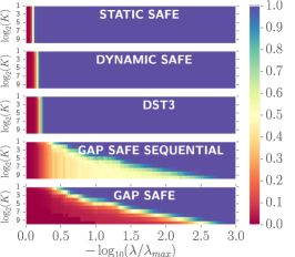
(b) Proportion of active group variables as a function of parameters $(\lambda_{t})$ and the number of iterations $K$.

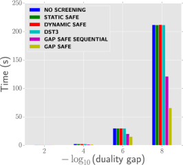
(c) Time to reach convergence as a function of increasing prescribed accuracy and using various screening strategies.

Figure 2: Experiments on a synthetic dataset ($\rho=0.5,\gamma_{1}=10,\gamma_{2}=4,\tau=0.2$).

Real dataset: NCEP/NCAR Reanalysis 1 Kalnay et al. (1996) The dataset contains monthly means of climate data measurements spread across the globe in a grid of $2.5^{\circ}\times 2.5^{\circ}$ resolutions (longitude and latitude $144\times 73$) from $1948/1/1$ to $2015/10/31$ . Each grid point constitutes a group of $7$ predictive variables (Air Temperature, Precipitable water, Relative humidity, Pressure, Sea Level Pressure, Horizontal Wind Speed and Vertical Wind Speed) whose concatenation across time constitutes our design matrix $X\in\mathbb{R}^{814\times 73577}$. Such data have therefore a natural group structure.

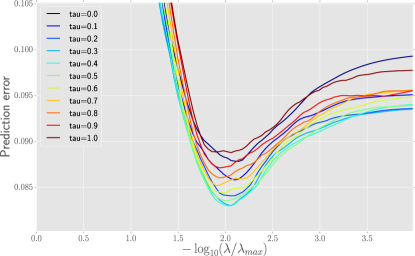
(a) We show the prediction error for the Sparse-Group Lasso path with $100$ values of $\lambda$ and $11$ values of $\tau$. The best performance is achieved with $\tau^{\star}=0.4$.

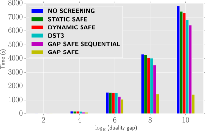
(b) We show the computation time to reach convergence as a function of the desired accuracy on the dual gap. The time includes the whole path over $(\lambda_{t})_{t\in[T]}$ with $\delta=2.5$ and $\tau^{\star}=0.4$.

      

Figure 3: Experiments on NCEP/NCAR Reanalysis 1 dataset (n = 814, p = 73577).

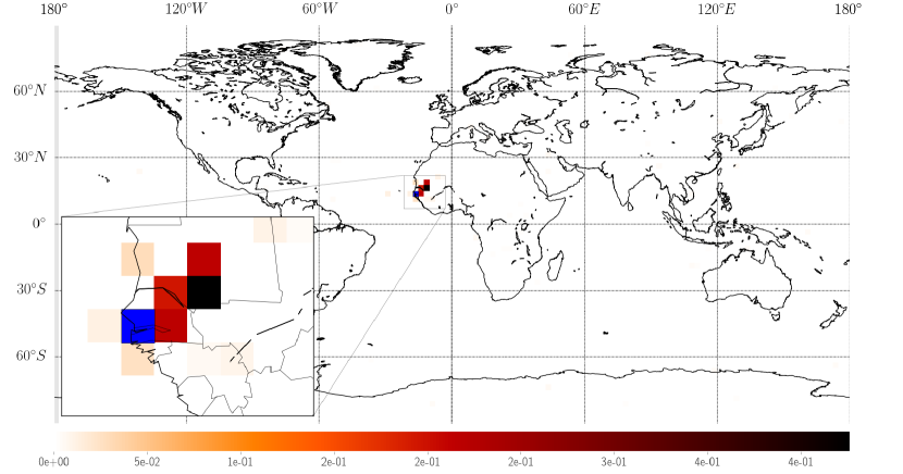
Figure 4: Experiments on NCEP/NCAR Reanalysis 1 dataset (n = 814, p = 73577). We show the active groups for the prediction of Air Temperature in a neighborhood of Dakar(location in blue). The regression coefficient are obtained by cross validation over $100$ values of $\lambda$ and $11$ values of $\tau$. At each location, we present the highest absolute value among the seven coefficients.

In our experiments, which aim to illustrate the computational benefit of the proposed method, we considered as target variable $y\in\mathbb{R}^{814}$, the values of Air Temperature in a neighborhood of Dakar. For preprocessing, we remove the seasonality and the trend present in the dataset. This is usually done in climate analysis to prevent some bias in the regression estimates. Similar data have been used in the past by Chatterjee et al. (2012), demonstrating that the Sparse-Group Lasso estimator is well suited for prediction in such climatology applications. Indeed, thanks to the sparsity structure the estimates delineate via their support some predictive regions at the group level, as well as predictive feature via coordinate-wise screening.

We choose the parameter $\tau$ in the set $\{0,0.1,\ldots,0.9,1\}$ by splitting in $50\%$ the observations and run a training-test validation procedure. For each value of $\tau$, we require a duality gap of $10^{-8}$ on the training part and pick the best one in term of prediction accuracy on the test part. The result is displayed in Figure 3(a). Since the prediction error degrades increasingly for $\lambda\leq\lambda_{\max}/10^{-2.5}$, we fix $\delta=2.5$ for the computational time benchmark in Figure 3(b).

7.2 Performance of the screening rules

In all our experiments, we observe that our proposed Gap Safe rule outperforms the other rules in term of computation time. On Figure 2(c), we can see that we need $65$s to reach convergence whereas others rules need up to $212$s at a precision of $10^{-8}$. A similar performance is observed on the real dataset (Figure 3(b)) where we obtain up to a $5$x speed up over the other rules. The key reason behind this performance gain is the convergence of the Gap Safe regions toward the dual optimal point as well as the efficient strategy to compute the screening rule. As shown in the results presented on Figure 2, our method still manages to screen out variables when $\lambda$ is small. It corresponds to low regularizations which lead to less sparse solutions but need to be explored during cross-validation.

In the climate experiments, the support map in Figure 4 shows that the most important coefficients are distributed in the vicinity of the target region (in agreement with our intuition). Nevertheless, some active variables with small coefficients remain and cannot be screened out.

Note that we do not compare our method to the TLFre (Wang & Ye, 2014), since this sequential rule requires the exact knowledge of the dual optimal solution which is not available in practice. As a consequence, one may discard active variables which can prevent the algorithm from converging as shown in (Ndiaye et al., 2015, Figure 4) for the Group-Lasso. This issue still occurs with the method explored by Lee & Xing (2014) for overlapping groups.

8 Conclusion

The recent GAP safe rules introduced in Fercoq et al. (2015); Ndiaye et al. (2015) for a wide range of regularized regression have shown great improvements in the reduction of computational burden specially in high dimension. A thorough investigation of the Sparse-Group Lasso norm allows us to generalize the GAP safe rule to the Sparse-Group Lasso problem. We give a new description of the dual feasible set by establishing a connection between the Sparse-Group Lasso norm and the $\epsilon$-norm. This new point of view on the geometry of the problem helps providing an efficient algorithm to compute the dual norm and dual feasible points. Extending GAP safe rules on more general hierarchical regularizations Wang & Ye (2015), is a possible direction for future research.

Appendix A Additional convexity and optimization tools

In what follows we will use the dot product notation for any $x,x^{\prime}\in\mathbb{R}^{d}$ we write $\langle x,x^{\prime}\rangle=x^{\top}x^{\prime}$.

We denote by $\iota_{C}$ the indicator function of a set $C$ defined as

$$\iota_{C}:\mathbb{R}^{d}\rightarrow\mathbb{R},\quad\iota_{C}(x)=\begin{cases}0,&\text{ if }x\in C,\\ +\infty,&\text{ otherwise.}\end{cases}$$ (24)

We denote by $f^{*}:\mathbb{R}^{d}\rightarrow\mathbb{R}$ the Fenchel conjugate of $f$ defined for any $z\in\mathbb{R}^{d}$ by $f^{*}(z)=\sup_{w\in\mathbb{R}^{d}}w^{\top}z-f(w)$.

Proposition 10.

(Bach et al. (2012, Prop. 1.4)) The Fenchel conjugate of the norm $\Omega$ is given by

$$\Omega^{*}(\xi)=\sup_{w\in\mathbb{R}^{d}}[\xi^{\top}w-\Omega(w)]=\iota_{\mathcal{B}_{\Omega^{D}}}(\xi).$$ (25)

Appendix B Proofs

Proposition 3 (Theoretical screening rules).

The two levels of screening rules for the Sparse-Group Lasso are:
Feature level screening:

$$\forall j\in g,\,|X_{j}^{\top}\hat{\theta}^{({\lambda,\tau,w})}|<\tau\Longrightarrow\hat{\beta}^{({\lambda,\tau,w})}_{j}=0.$$

Group level screening:

$$\forall g\in\mathcal{G},\,\|\mathcal{S}_{\tau}(X_{g}^{\top}\hat{\theta}^{({\lambda,\tau,w})})\|<(1-\tau)w_{g}\Longrightarrow\hat{\beta}^{({\lambda,\tau,w})}_{g}=0.$$

Proof.

Let us consider $\hat{\beta}^{({\lambda,\tau,w})}_{g}\neq 0$, $g\in\mathcal{G}$. Then combining the subdifferential inclusion (8), the subdifferential of the $\ell_{2}$-norm (2) and the decomposition of any dual feasible point (8), we obtain :

$$X_{g}^{\top}\hat{\theta}^{({\lambda,\tau,w})} =\tau v_{g}+(1-\tau)w_{g}\frac{\hat{\beta}^{({\lambda,\tau,w})}_{g}}{\left\lVert\hat{\beta}^{({\lambda,\tau,w})}\right\rVert}\text{ where }v\in\partial\left\lVert\cdot\right\rVert_{1}(\hat{\beta}^{({\lambda,\tau,w})}),$$

$$X_{g}^{\top}\hat{\theta}^{({\lambda,\tau,w})} =\Pi_{\tau\mathcal{B}_{\infty}}(X_{g}^{\top}\hat{\theta}^{({\lambda,\tau,w})})+\mathcal{S}_{{\tau}}(X_{g}^{\top}\hat{\theta}^{({\lambda,\tau,w})}).$$

So we can deduce that $\mathcal{S}_{{\tau}}(X_{g}^{\top}\hat{\theta}^{({\lambda,\tau,w})})\in(1-\tau)w_{g}\left\{\frac{\hat{\beta}^{({\lambda,\tau,w})}_{g}}{\left\lVert\hat{\beta}^{({\lambda,\tau,w})}_{g}\right\rVert}\right\}$. Since $\hat{\theta}^{({\lambda,\tau,w})}$ is feasible then $\|\mathcal{S}_{{\tau}}(X_{g}^{\top}\hat{\theta}^{({\lambda,\tau,w})})\|<(1-\tau)w_{g}$ is equivalent to $\|\mathcal{S}_{{\tau}}(X_{g}^{\top}\hat{\theta}^{({\lambda,\tau,w})})\|\neq(1-\tau)w_{g}$ which implies, by contrapositive, that $\hat{\beta}^{({\lambda,\tau,w})}_{g}=0$. Hence we obtain the group level safe rule. Furthermore, from the subdifferential of the $\ell_{1}$-norm (1), we have:

$$\forall j\in g,\,X_{j}^{\top}\hat{\theta}^{({\lambda,\tau,w})}\in\begin{cases}(1-\tau)w_{g}\left\{\frac{\hat{\beta}^{({\lambda,\tau,w})}_{j}}{\|\hat{\beta}^{({\lambda,\tau,w})}\|}\right\}+\tau\left\{\operatorname{sign}(\hat{\beta}^{({\lambda,\tau,w})}_{j})\right\},&\text{ if }\hat{\beta}^{({\lambda,\tau,w})}_{j}\neq 0,\\ [-\tau,\tau],&\text{ if }\hat{\beta}^{({\lambda,\tau,w})}_{j}=0.\end{cases}$$

Hence, if $\hat{\beta}^{({\lambda,\tau,w})}_{j}\neq 0$ then $X_{j}^{\top}\hat{\theta}^{({\lambda,\tau,w})}=\operatorname{sign}(\hat{\beta}^{({\lambda,\tau,w})}_{j})\left[(1-\tau)w_{g}\frac{|\hat{\beta}^{({\lambda,\tau,w})}_{j}|}{\|\hat{\beta}^{({\lambda,\tau,w})}\|}+\tau\right]$ and so $|X_{j}^{\top}\hat{\theta}^{({\lambda,\tau,w})}|\geq\tau$. By contrapositive, we obtain the feature level safe rule. ∎

Proposition 4.

For all group $g\in\mathcal{G}$ and $j\in g$,

$$\max_{\theta\in\mathcal{B}(\theta_{c},r)}|X_{j}^{\top}\theta|\leq|X_{j}^{\top}\theta_{c}|+r\|X_{j}\|.$$ (26)

$\max_{\theta\in\mathcal{B}(\theta_{c},r)}\|\mathcal{S}_{{\tau}}(X_{g}^{\top}\theta)\|$ is upper bounded by

$$\begin{cases}\|\mathcal{S}_{{\tau}}(X_{g}^{\top}\theta_{c})\|+r\|X_{g}\|&\text{ if }\|X_{g}^{\top}\theta_{c}\|_{\infty}>\tau,\\ (\|X_{g}^{\top}\theta_{c}\|_{\infty}+r\|X_{g}\|-\tau)_{+}&\text{ otherwise}.\end{cases}$$ (27)

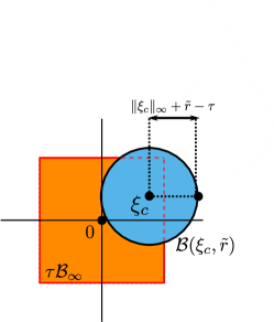
(a) $\mathcal{B}(\xi_{c},\tilde{r})\cap\tau\mathcal{B}_{\infty}\neq\emptyset$; $\xi_{c}\in\tau\mathring{\mathcal{B}_{\infty}}$

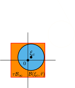
(b) $\mathcal{B}(\xi_{c},\tilde{r})\subset\tau\mathcal{B}_{\infty}$

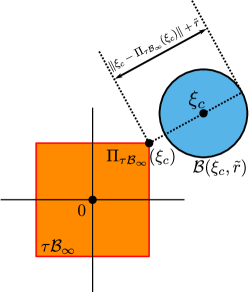
(c) $\mathcal{B}(\xi_{c},\tilde{r})\cap\tau\mathcal{B}_{\infty}=\emptyset$; $\xi_{c}\notin\tau\mathring{\mathcal{B}_{\infty}}$

Proof.

$|X_{j}^{\top}\theta|\leq|[X_{g}^{\top}(\theta-\theta_{c})]_{j}|+|X_{j}^{\top}\theta_{c}|\leq r\|X_{j}\|+|X_{j}^{\top}\theta_{c}|$ as soon as $\theta\in\mathcal{B}(\theta_{c},r)$.

Since $\theta\in\mathcal{B}(\theta_{c},r)$ implies that $X_{g}^{\top}\theta\in\mathcal{B}(X_{g}^{\top}\theta_{c},r\|X_{g}\|)$, we have $\max_{\theta\in\mathcal{B}(\theta_{c},r)}\|\mathcal{S}_{{\tau}}(X_{g}^{\top}\theta)\|\leq\max_{\xi\in\mathcal{B}(\xi_{c},\tilde{r})}\|\mathcal{S}_{{\tau}}(\xi)\|$ where $\xi_{c}=X_{g}^{\top}\theta_{c}$ and $\tilde{r}=r\left\lVert X_{j}\right\rVert$. From now, we just have to show how to compute $\max_{\xi\in\mathcal{B}(\xi_{c},\tilde{r})}\|\mathcal{S}_{{\tau}}(\xi)\|$.

• In the case where $\xi_{c}\in\mathring{\tau\mathcal{B}_{\infty}}$, if $\|\xi_{c}\|_{\infty}+\tilde{r}\leq\tau\,(\text{ {\em i.e.,~{}}}\mathcal{B}(\xi_{c},\tilde{r})\subset\tau\mathcal{B}_{\infty})$, we have $\Pi_{\tau\mathcal{B}_{\infty}}(\xi)=\xi$ and thus, $\max_{\xi\in\mathcal{B}(\xi_{c},\tilde{r})}\|\mathcal{S}_{{\tau}}(\xi)\|=\max_{\xi\in\mathcal{B}(\xi_{c},\tilde{r})}\|\xi-\Pi_{\tau\mathcal{B}_{\infty}}(\xi)\|=0.$

• Otherwise if $\xi_{c}\in\mathring{\tau\mathcal{B}_{\infty}}$ and $\|\xi_{c}\|_{\infty}+\tilde{r}>\tau$, for any vector $\xi\in\partial\mathcal{B}(\xi_{c},\tilde{r})\cap(\tau\mathcal{B}_{\infty})^{c}$ and any vector $\tilde{\xi}\in\partial\tau\mathcal{B}_{\infty}\cap[\xi,\xi_{c}]$, $\|\xi-\Pi_{\tau\mathcal{B}_{\infty}}(\xi)\|\leq\|\xi-\tilde{\xi}\|=\tilde{r}-\|\tilde{\xi}-\xi_{c}\|$. Hence

  $$\max_{\xi\in\mathcal{B}(\xi_{c},\tilde{r})}\|\xi-\Pi_{\tau\mathcal{B}_{\infty}}(\xi)\|\leq\max_{\underset{\tilde{\xi}\in\partial\tau\mathcal{B}_{\infty}\cap[\xi,\xi_{c}]}{\xi\in\partial\mathcal{B}(\xi_{c},\tilde{r})\cap(\tau\mathcal{B}_{\infty})^{c}}}\tilde{r}-\|\tilde{\xi}-\xi_{c}\|\leq\tilde{r}-\min_{\xi\in\partial\tau\mathcal{B}_{\infty}}\|\xi-\xi_{c}\|=\tilde{r}-\tau+\|\xi_{c}\|_{\infty}.$$

  This upper bound is attained. Indeed, $\max_{\theta\in\mathcal{B}(\xi_{c},\tilde{r})}\|\xi-\Pi_{\tau\mathcal{B}_{\infty}}(\xi)\|=\tilde{r}-\|\Pi_{\tau\mathcal{B}_{\infty}}(\hat{\xi})-\xi_{c}\|=\tilde{r}-\tau+\|\xi_{c}\|_{\infty}$ where $\hat{\xi}$ is a vector in $\partial\mathcal{B}(\xi_{c},\tilde{r})$ such that $\Pi_{\tau\mathcal{B}_{\infty}}(\hat{\xi})=\xi_{c}+e_{j^{\star}}(\tau-\|\xi_{c}\|_{\infty})$ and $j^{\star}\in\mathop{\mathrm{arg\,max}}_{j\in[p]}|(\xi_{c})_{j}|$.

• If $\xi_{c}\notin\mathring{\tau\mathcal{B}_{\infty}}$, since the projection operator on a convex set is a contraction, we have

  $$\forall\xi\in\partial\mathcal{B}(\xi_{c},\tilde{r}),\,\|\xi-\Pi_{\tau\mathcal{B}_{\infty}}(\xi)\|\leq\|\xi-\Pi_{\tau\mathcal{B}_{\infty}}(\xi_{c})\|\leq\|\xi_{c}-\Pi_{\tau\mathcal{B}_{\infty}}(\xi_{c})\|+\|\xi-\xi_{c}\|=\|\xi_{c}-\Pi_{\tau\mathcal{B}_{\infty}}(\xi_{c})\|+\tilde{r}.$$

  Moreover, it is straightforward to see that the vector $\tilde{\xi}:=\tilde{\gamma}\xi_{c}+(1-\tilde{\gamma})\Pi_{\tau\mathcal{B}_{\infty}}(\xi_{c})$ where $\tilde{\gamma}=1+\frac{\tilde{r}}{\left\lVert\xi_{c}\right\rVert+\left\lVert\Pi_{\tau\mathcal{B}_{\infty}}(\xi_{c})\right\rVert}$ belongs to $\partial\mathcal{B}(\xi_{c},\tilde{r})$; it verifies $\Pi_{\tau\mathcal{B}_{\infty}}(\xi_{c})=\Pi_{\tau\mathcal{B}_{\infty}}(\tilde{\xi})$ and it attains this bound. ∎

Theorem 2 (Safe radius).

For any $\theta\in\Delta_{X,\Omega_{\tau,w}}$ and any $\beta\in\mathbb{R}^{p}$, one has $\hat{\theta}^{({\lambda,\tau,w})}\in\mathcal{B}\left(\theta,{r}_{\lambda,\tau}(\beta,\theta)\right),$ for

$${r}_{\lambda,\tau}(\beta,\theta) =\sqrt{\frac{2(P_{\lambda,\tau,w}(\beta)-D_{\lambda}(\theta))}{\lambda^{2}}},$$

i.e., the aforementioned ball is a safe region for the Sparse-Group Lasso problem.

Proof.

By weak duality, $\forall\beta\in\mathbb{R}^{p},\,D_{\lambda}(\hat{\theta}^{({\lambda,\tau,w})})\leq P_{\lambda,\tau,w}(\beta)$. Then, note that the dual objective function (5) is $\lambda^{2}$-strongly concave. This implies:

$$\forall(\theta,\theta^{\prime})\in\Delta_{X,\Omega_{\tau,w}}\times\Delta_{X,\Omega_{\tau,w}},\quad D_{\lambda}(\theta)\leq D_{\lambda}(\theta^{\prime})+\nabla D_{\lambda}(\theta^{\prime})^{\top}(\theta-\theta^{\prime})-\frac{\lambda^{2}}{2}\left\lVert\theta-\theta^{\prime}\right\rVert^{2}.$$

Moreover, since $\hat{\theta}^{({\lambda,\tau,w})}$ maximizes the concave function $D_{\lambda}$, the following inequality holds true:

$$\forall\,\theta\in\Delta_{X,\Omega_{\tau,w}},\quad\nabla D_{\lambda}(\hat{\theta}^{({\lambda,\tau,w})})^{\top}(\theta-\hat{\theta}^{({\lambda,\tau,w})})\leq 0.$$

Hence, we have for all $\theta\in\Delta_{X,\Omega_{\tau,w}}$ and $\beta\in\mathbb{R}^{p}$:

$$\frac{\lambda^{2}}{2}\|\theta-\hat{\theta}^{({\lambda,\tau,w})}\|^{2} \leq D_{\lambda}(\hat{\theta}^{({\lambda,\tau,w})})-D_{\lambda}(\theta)$$

$$\leq P_{\lambda,\tau,w}(\beta)-D_{\lambda}(\theta).\qed$$

Proposition 5.

If $\lim_{k\to\infty}\beta_{k}=\hat{\beta}^{({\lambda,\tau,w})}$, then $\lim_{k\to\infty}\theta_{k}=\hat{\theta}^{({\lambda,\tau,w})}$.

Proof.

Let $\alpha_{k}=\max(\lambda,\Omega_{\tau,w}^{D}(X^{\top}\rho_{k}))$ and recall that $\rho_{k}=y-X\beta_{k}$. We have :

$$\left\lVert\theta_{k}-\hat{\theta}^{({\lambda,\tau,w})}\right\rVert =\left\lVert\frac{1}{\alpha_{k}}(y-X\beta_{k})-\frac{1}{\lambda}(y-X\hat{\beta}^{({\lambda,\tau,w})})\right\rVert$$

$$=\left\lVert\left(\frac{1}{\alpha_{k}}-\frac{1}{\lambda}\right)(y-X\beta_{k})-\frac{(X\hat{\beta}^{({\lambda,\tau,w})}-X\beta_{k})}{\lambda}\right\rVert$$

$$\leq\left|\frac{1}{\alpha_{k}}-\frac{1}{\lambda}\right|\left\lVert y-X\beta_{k}\right\rVert+\left\lVert\frac{X\hat{\beta}^{({\lambda,\tau,w})}-X\beta_{k}}{\lambda}\right\rVert.$$

If $\beta_{k}\rightarrow\hat{\beta}^{({\lambda,\tau,w})}$, then $\alpha_{k}\rightarrow\max(\lambda,\Omega_{\tau,w}^{D}(X^{\top}(y-X\hat{\beta}^{({\lambda,\tau,w})}))=\max(\lambda,\lambda\Omega_{\tau,w}^{D}(X^{\top}\hat{\theta}^{({\lambda,\tau,w})}))=\lambda$ since $y-X\hat{\beta}^{({\lambda,\tau,w})}=\lambda\hat{\theta}^{({\lambda,\tau,w})}$ thanks to the link-equation (7) and since $\hat{\theta}^{({\lambda,\tau,w})}$ is feasible i.e., $\Omega_{\tau,w}^{D}(X^{\top}\hat{\theta}^{({\lambda,\tau,w})})\leq 1$. Hence, both terms in the previous inequality converge to zero. ∎

Proposition 6.

Let $(\mathcal{R}_{k})_{k\in\mathbb{N}}$ be a sequence of safe regions whose diameters converge to 0. Then, $\displaystyle\lim_{k\rightarrow\infty}\mathcal{A}_{\text{groups}}(\mathcal{R}_{k})=\mathcal{E}_{\text{groups}}$ and $\displaystyle\lim_{k\rightarrow\infty}\mathcal{A}_{\text{features}}(\mathcal{R}_{k})=\mathcal{E}_{\text{features}}$.

Proof.

We proceed by double inclusion. First let us prove that $\exists k_{0}$ s.t. $\forall k\geq k_{0},\mathcal{A}_{\text{groups}}(\mathcal{R}_{k})\subset\mathcal{E}_{\text{groups}}$. Indeed, since the diameter of $\mathcal{R}_{k}$ converges to zero, for any $\epsilon>0$ there exist $k_{0}\in\mathbb{N},\forall k\geq k_{0},\forall\theta\in\mathcal{R}_{k},\|\theta-\hat{\theta}^{({\lambda,\tau,w})}\|\leq\epsilon$. The triangle inequality implies that $\forall g\notin\mathcal{E}_{\text{groups}}$, $\|\mathcal{S}_{{\tau}}(X_{g}^{\top}\theta)\|\leq\|\mathcal{S}_{{\tau}}(X_{g}^{\top}\theta)-\mathcal{S}_{{\tau}}(X_{g}^{\top}\hat{\theta}^{({\lambda,\tau,w})})\|+\|\mathcal{S}_{{\tau}}(X_{g}^{\top}\hat{\theta}^{({\lambda,\tau,w})})\|$. Since the soft-thresholding operator is $1$-Lipschitz, we have:

$$\|\mathcal{S}_{{\tau}}(X_{g}^{\top}\theta)\|\leq\|X_{g}(\theta-\hat{\theta}^{({\lambda,\tau,w})})\|+\|\mathcal{S}_{{\tau}}(X_{g}^{\top}\hat{\theta}^{({\lambda,\tau,w})})\|\leq\epsilon\|X_{g}\|+\|\mathcal{S}_{{\tau}}(X_{g}^{\top}\hat{\theta}^{({\lambda,\tau,w})})\|,$$

as soon as $k\geq k_{0}$. Moreover, $\forall g\notin\mathcal{E}_{\text{groups}}$,

$$\|\mathcal{S}_{{\tau}}(X_{g}^{\top}\theta)\|\leq\max_{g\notin\mathcal{E}_{\text{groups}}}\|\mathcal{S}_{{\tau}}(X_{g}^{\top}\theta)\|\leq\epsilon\max_{g\notin\mathcal{E}_{\text{groups}}}\|X_{g}\|+\max_{g\notin\mathcal{E}_{\text{groups}}}\|\mathcal{S}_{{\tau}}(X_{g}^{\top}\hat{\theta}^{({\lambda,\tau,w})})\|.$$

It suffices to choose $\epsilon$ such that

$$\epsilon\max_{g\notin\mathcal{E}_{\text{groups}}}\|X_{g}\|+\max_{g\notin\mathcal{E}_{\text{groups}}}\|\mathcal{S}_{{\tau}}(X_{g}^{\top}\hat{\theta}^{({\lambda,\tau,w})})\|<(1-\tau)w_{g},$$

that is to say $\epsilon<\frac{(1-\tau)w_{g}-\max_{g\notin\mathcal{E}_{\text{groups}}}\|\mathcal{S}_{{\tau}}(X_{g}^{\top}\hat{\theta}^{({\lambda,\tau,w})})\|}{\max_{g\notin\mathcal{E}_{\text{groups}}}\|X_{g}\|}$, to remove the group $g$. For any $k\geq k_{0},\,\mathcal{E}_{\text{groups}}^{c}=\{g\in\mathcal{G}:\|\mathcal{S}_{\tau}(X_{g}^{\top}\hat{\theta}^{({\lambda})})\|<(1-\tau)w_{g}\}\subset\mathcal{A}_{\text{groups}}(\mathcal{R}_{k})^{c}$, the set of variables removed by our screening rule. This proves the first inclusion.

Now we show that $\forall k\in\mathbb{N},\mathcal{A}_{\text{groups}}(\mathcal{R}_{k})\supset\mathcal{E}_{\text{groups}}$. Indeed, for all $g^{\star}\in\mathcal{E}_{\text{groups}}$, $\|\mathcal{S}_{{\tau}}(X_{g^{\star}}^{T}\hat{\theta}^{({\lambda,\tau,w})})\|=(1-\tau)w_{g^{\star}}$. Since for all $k$ in $\mathbb{N}$, $\hat{\theta}^{({\lambda,\tau,w})}\in\mathcal{R}_{k}$ then $\underset{\theta\in\mathcal{R}_{k}}{\max}\|\mathcal{S}_{{\tau}}(X_{g}^{\top}\theta)\|\geq\|\mathcal{S}_{{\tau}}(X_{g^{\star}}^{T}\hat{\theta}^{({\lambda,\tau,w})})\|=(1-\tau)w_{g^{\star}}$ hence the second inclusion holds.

We have shown that that $\forall k\geq k_{0}$ $\mathcal{A}_{\text{groups}}(\mathcal{R}_{k})=\mathcal{E}_{\text{groups}}$ and so $\mathcal{A}_{\text{features}}(\mathcal{R}_{k})\subset\bigcup_{g\in\mathcal{E}_{\text{groups}}}\left\{j\in g:\,\max_{\theta\in\mathcal{R}_{k}}|X_{j}^{\top}\theta|\geq\tau\right\}$. Moreover, the same reasoning yields $\forall g\in\mathcal{G}$, $\left\{j\in g:\,\max_{\theta\in\mathcal{R}_{k}}|X_{j}^{\top}\theta|\geq\tau\right\}\subset\left\{j\in g:\,|X_{j}^{\top}\hat{\theta}^{({\lambda,\tau,w})}|\geq\tau\right\}$. Hence $\forall k\geq k_{0},\mathcal{A}_{\text{features}}(\mathcal{R}_{k})\subset\mathcal{A}_{\text{features}}$. The reciprocal inclusion is straightforward. ∎

Proposition 7.

. For all group $g$ in $\mathcal{G}$, let $\epsilon_{g}:=\frac{(1-\tau)w_{g}}{\tau+(1-\tau)w_{g}}$ then the Sparse-Group Lasso norm satisfies the following properties: for any vectors $\beta$ and $\xi$ in $\mathbb{R}^{p}$

$$\Omega_{\tau,w}(\beta)=\sum_{g\in\mathcal{G}}(\tau+(1-\tau)w_{g})\|\beta_{g}\|_{\epsilon_{g}}^{D}$$ (28)

$$\Omega_{\tau,w}^{D}(\xi)=\max_{g\in\mathcal{G}}\frac{\left\lVert\xi_{g}\right\rVert_{\epsilon_{g}}}{\tau+(1-\tau)w_{g}}.$$ (29)

$$\mathcal{B}_{\Omega_{\tau,w}^{D}}=\big{\{}\xi\in\mathbb{R}^{p}:\forall g\in\mathcal{G},\|\mathcal{S}_{{\tau}}(\xi_{g})\|\leq(1-\tau)w_{g}\big{\}}$$ (30)

The subdifferential $\partial\Omega_{\tau,w}(\beta)$ of the norm $\Omega_{\tau,w}$ at $\beta$ is given by

$$\bigg{\{}x\in\mathbb{R}^{p}:\forall g\in\mathcal{G},x_{g}\in\tau\partial\|\cdot\|_{1}(\beta_{g})+(1-\tau)w_{g}\partial\|\cdot\|(\beta_{g})\bigg{\}}$$

Proof.

$$\forall\beta\in\mathbb{R}^{p},\,\Omega(\beta) =\tau\|\beta\|_{1}+(1-\tau)\sum_{g\in\mathcal{G}}w_{g}\|\beta_{g}\|=\sum_{g\in\mathcal{G}}\big{(}\tau\|\beta_{g}\|_{1}+(1-\tau)w_{g}\|\beta_{g}\|\big{)}$$

$$=\sum_{g\in\mathcal{G}}(\tau+(1-\tau)w_{g})\left[\frac{\tau}{\tau+(1-\tau)w_{g}}\|\beta_{g}\|_{1}+\frac{(1-\tau)w_{g}}{\tau+(1-\tau)w_{g}}\|\beta_{g}\|\right]$$

$$=\sum_{g\in\mathcal{G}}(\tau+(1-\tau)w_{g})\left[(1-\epsilon_{g})\|\beta_{g}\|_{1}+\epsilon_{g}\|\beta_{g}\|\right]=\sum_{g\in\mathcal{G}}(\tau+(1-\tau)w_{g})\|\beta_{g}\|_{\epsilon_{g}}^{D}$$

The definition of the dual norm reads $\displaystyle\Omega^{D}(\xi)=\max_{\beta:\Omega(\beta)\leq 1}\beta^{\top}\xi$, and solving this problem yields:

$$\Omega^{D}(\xi) =\sup_{\beta:\Omega(\beta)\leq 1}\langle\beta,\xi\rangle=\sup_{\beta}\inf_{\mu>0}\langle\beta,\sum_{g\in\mathcal{G}}\xi_{g}\rangle-\mu\left(\sum_{g\in\mathcal{G}}\Omega_{g}(\beta_{g})-1\right)$$

$$=\inf_{\mu>0}\left\{\sum_{g\in\mathcal{G}}\sup_{\beta_{g}}\left[\langle\beta_{g},\xi_{g}\rangle-\mu\Omega_{g}(\beta_{g})\right]+\mu\right\}$$

$$=\inf_{\mu>0}\left\{\sum_{g\in\mathcal{G}}\mu\Omega_{g}^{*}\left(\frac{\xi_{g}}{\mu}\right)+\mu\right\}=\inf_{\mu>0}\left\{\sum_{g\in\mathcal{G}}\iota_{\mathcal{B}_{\Omega_{g}^{D}}}\left(\frac{\xi_{g}}{\mu}\right)+\mu\right\}$$

$$=\inf_{\mu>0}\left\{\max_{g\in\mathcal{G}}\iota_{\mathcal{B}_{\Omega_{g}^{D}}}\left(\frac{\xi_{g}}{\mu}\right)+\mu\right\}=\max_{g\in\mathcal{G}}\inf_{\mu>0}\left\{\Omega_{g}^{*}\left(\frac{\xi_{g}}{\mu}\right)+\mu\right\}$$

$$=\max_{g\in\mathcal{G}}\inf_{\mu>0}\sup_{\beta_{g}}\langle\beta_{g},\frac{\xi_{g}}{\mu}\rangle-\Omega_{g}(\beta_{g})+\mu\underset{\mu u_{g}=\beta_{g}}{=}\max_{g\in\mathcal{G}}\inf_{\mu>0}\sup_{u_{g}}\langle u_{g},\xi_{g}\rangle-\mu(\Omega_{g}(u_{g})-1)$$

$$=\max_{g\in\mathcal{G}}\sup_{u_{g}:\Omega_{g}(u_{g})\leq 1}\langle u_{g},\xi_{g}\rangle=\max_{g\in\mathcal{G}}\sup_{u_{g}}\,\langle u_{g},\xi_{g}\rangle\quad\text{ s.t. }(\tau+(1-\tau)w_{g})\left\lVert u_{g}\right\rVert_{\epsilon_{g}}^{D}\leq 1$$

$$=\max_{g\in\mathcal{G}}\sup_{u_{g}:\Omega_{g}(u_{g})\leq 1}\langle u_{g},\xi_{g}\rangle=\max_{g\in\mathcal{G}}\sup_{{u^{\prime}}_{g}:\left\lVert{u^{\prime}}_{g}\right\rVert_{\epsilon_{g}}^{D}\leq 1}\langle\frac{{u^{\prime}}_{g}}{\tau+(1-\tau)w_{g}},\xi_{g}\rangle=\max_{g\in\mathcal{G}}\frac{\left\lVert\xi_{g}\right\rVert_{\epsilon_{g}}}{\tau+(1-\tau)w_{g}}.$$

We recall here the proof of Wang & Ye (2014) for the sake of completeness. First let us write $\Omega(\beta)=\Omega_{1}(\beta)+\Omega_{2}(\beta)$, where $\Omega_{1}(\beta)=\tau\left\lVert\beta\right\rVert_{1}$ and $\Omega_{2}(\beta)=(1-\tau)\sum_{g\in\mathcal{G}}w_{g}\left\lVert\beta_{g}\right\rVert_{2}$. Since $\Omega_{1}$ and $\Omega_{2}$ are continuous everywhere, we have (see Hiriart-Urruty (2006, Theorem 1)): $\Omega^{*}(\xi)=(\Omega_{1}+\Omega_{2})^{*}(\xi)=\min_{a+b=\xi}[\Omega_{1}^{*}(a)+\Omega_{2}^{*}(b)]=\min_{a}[\Omega_{1}^{*}(a)+\Omega_{2}^{*}(\xi-a)]$, which is also the inf-convolution (see Bauschke & Combettes (2011, Chapter 12)) of these two norms. Using the Fenchel conjugate of the $\ell_{1}$ norm ($\Omega_{1}^{*}=\iota_{\tau\mathcal{B}_{\infty}}$) and of the $\ell_{2}$ norm ($\Omega_{2}^{*}=\iota_{\mathcal{B}}$), we have

$$\Omega^{*}(\xi)=\sum_{g\in\mathcal{G}}\min_{a_{g}}\iota_{\tau\mathcal{B}_{\infty}}(a_{g})+\iota_{\mathcal{B}}\left(\frac{\xi_{g}-a_{g}}{(1-\tau)w_{g}}\right)=\sum_{g\in\mathcal{G}}\iota_{\mathcal{B}}\left(\frac{\xi_{g}-\Pi_{\tau\mathcal{B}_{\infty}}(\xi_{g})}{(1-\tau)w_{g}}\right).$$

Hence the indicator of the unit dual ball is $\iota_{\mathcal{B}_{\Omega^{D}}}(\xi)=\sum_{g\in\mathcal{G}}\iota_{(1-\tau)w_{g}\mathcal{B}}\left(\xi_{g}-\Pi_{\tau\mathcal{B}_{\infty}}(\xi_{g})\right)$ and using $\mathcal{S}_{{\tau}}(\xi_{g})=\xi_{g}-\Pi_{\tau\mathcal{B}_{\infty}}$, we have:

$$\mathcal{B}_{\Omega^{D}}=\big{\{}\xi\in\mathbb{R}^{p}:\Omega^{D}(\xi)\leq 1\big{\}}=\big{\{}\xi\in\mathbb{R}^{p}:\forall g\in\mathcal{G},\,\|\mathcal{S}_{{\tau}}(\xi_{g})\|\leq(1-\tau)w_{g}\big{\}}.$$

∎

Proposition 9.

. For $\alpha\in[0,1],R\geq 0$ and $x\in\mathbb{R}^{d}$, the equation $\sum_{j=1}^{d}\mathcal{S}_{{\nu\alpha}}(x_{j})^{2}=(\nu R)^{2}$ has a unique solution $\nu\in\mathbb{R}_{+}$, denoted by $\Lambda(x,\alpha,R)$ and that can be computed in $O(d\log d)$ operations in worst case.

Proof.

Dividing by $\nu^{2}$, which is positive as soon as $x\neq 0$, we get that $\sum_{j=1}^{d}\mathcal{S}_{{\nu\alpha}}(x_{j})^{2}=(\nu R)^{2}$ is equivalent to $\sum_{j=1}^{d}\mathcal{S}_{{\alpha}}(x_{j}/\nu)^{2}=R^{2}$. Note that $\sum_{j=1}^{d}\mathcal{S}_{{\alpha}}(x_{j}/\nu)^{2}=\sum_{j=1}^{d}\mathcal{S}_{{\alpha}}(|x_{j}|/\nu)^{2}$ so without loss of generality we assume $x\in\mathbb{R}_{+}^{d}$.

The case $\alpha=0$ and $R=0$ corresponds to the situation where all $x_{j}$ are equal to zero or we impose $\nu$ equals to infinity. So we avoid this trivial case.

If $\alpha=0$ and $R\neq 0$, $\nu=\|x\|/R$. Indeed,

$$\sum_{j=1}^{d}\mathcal{S}_{{0}}(x_{j}/\nu)^{2}=R^{2}\Longleftrightarrow\sum_{j=1}^{d}(x_{j}/\nu)^{2}=R^{2}\Longleftrightarrow\frac{\|x\|_{2}^{2}}{\nu^{2}}=R^{2}\text{ hence the result}.$$

If $\alpha\neq 0$ and $R=0$, we have :

$$\sum_{j=1}^{d}\mathcal{S}_{{\alpha}}\left(\frac{x_{j}}{\nu}\right)^{2}=0\Longleftrightarrow\forall j\in[d],\left(\frac{x_{j}}{\nu}-\alpha\right)_{+}=0\Longleftrightarrow\forall j\in[d],\frac{x_{j}}{\nu}\leq\alpha\Longleftrightarrow\nu\geq\frac{\max_{j\in[d]}x_{j}}{\alpha}.$$

So we choose the smallest $\nu$ i.e., $\nu=\|x\|_{\infty}/\alpha$. In all the above cases, the computation is done in $O(d)$.

Otherwise $\alpha\neq 0$ and $R\neq 0$. The function $\nu\mapsto\sum_{j=1}^{d}\mathcal{S}_{{\alpha}}(x_{j}/\nu)^{2}$ is a non-increasing continuous function with limit $+\infty$ (resp. $0$) when $\nu\to 0$ (resp. $\nu\to+\infty$). Hence, there is a unique solution to $\sum_{j=1}^{d}\mathcal{S}_{{\alpha}}(x_{j}/\nu)^{2}=R^{2}$.

We denote by $x_{(1)},\dots,x_{(d)}$ the coordinates of $x$ ordered in decreasing order (with the convention $x_{(0)}=+\infty$ and $x_{(d+1)}=0$). Note that $\sum_{j=1}^{d}\mathcal{S}_{{\alpha}}(x_{j}/\nu)^{2}=\sum_{j=1}^{d}\mathcal{S}_{{\alpha}}(x_{(j)}/\nu)^{2}$. Then, there exists an index $j_{0}\in[p]$ such that

$$R^{2}\in\left[\sum_{j=0}^{d}\mathcal{S}_{{\alpha}}\left(\alpha\frac{x_{(j)}}{x_{(j_{0})}}\right)^{2},\sum_{j=0}^{d}\mathcal{S}_{{\alpha}}\left(\alpha\frac{x_{(j)}}{x_{(j_{0}+1)}}\right)^{2}\right).$$ (31)

For such a $j_{0}$, one can check that $\nu\in(x_{(j_{0}+1)}/\alpha,x_{(j_{0})}/\alpha]$. The definition of the soft-thresholding operator yields

$$\mathcal{S}_{{\alpha}}(x_{j}/\nu)^{2}=\begin{cases}(x_{j}/\nu-\alpha)^{2}&\text{if }x_{j}\geq\nu\alpha,\\ 0&\text{if }x_{j}<\nu\alpha.\end{cases}$$ (32)

It can be simplified thanks to $x_{j}\geq x_{(j_{0})}\Rightarrow x_{j}\geq\nu\alpha$ and $x_{j}\leq x_{(j_{0}+1)}\Rightarrow x_{j}<\nu\alpha$. Hence, $R^{2}=\sum_{j=1}^{j_{0}}(x_{(j)}/\nu-\alpha)^{2}=\sum_{j=1}^{j_{0}}(x_{(j)}/\nu)^{2}+\alpha^{2}\sum_{j=1}^{j_{0}}1-2\alpha\sum_{j=1}^{j_{0}}x_{(j)}/\nu$ so solving $\sum_{j=1}^{p}\mathcal{S}_{{\alpha}}(x_{(j)}/\nu)^{2}=R^{2}$ is equivalent to solve on $\mathbb{R}_{+}$

$$(\alpha^{2}j_{0}-R^{2})\nu^{2}-\left(2\alpha\sum_{j=1}^{j_{0}}x_{(j)}\right)\nu+\sum_{j=1}^{j_{0}}x_{(j)}^{2}=0.$$ (33)

If $(\alpha^{2}j_{0}-R^{2})=0$, then $\nu=\sum_{j=1}^{j_{0}}x_{(j)}^{2}/(2\alpha\sum_{j=1}^{j_{0}}x_{(j)})$. Otherwise $\nu$ is the unique solution lying in $(x_{(j_{0}+1)}/\alpha,x_{(j_{0})}/\alpha]$ of the quadratic equation stated in Eq. (33).

In the worst case, to compute $\Lambda(x,\alpha,R)$, one needs to sort a vector of size $d$, what can be done in $O(d\log(d))$ operations, and finding $j_{0}$ thanks to (31) requires $O(d^{2})$ if we apply a naive algorithm.

In the following, we show that one can easily reduce the complexity to $O(d\log(d))$ in worst case.

For all $j$ in $[d],\,\mathcal{S}_{{\alpha}}\left(\alpha\frac{x_{j}}{x_{j_{0}}}\right)=0$ as soon as $x_{j}\leq x_{j_{0}}$. This implies that (31) is equivalent to

$$R^{2}\in\left[\sum_{j=0}^{j_{0}-1}\mathcal{S}_{{\alpha}}\left(\alpha\frac{x_{(j)}}{x_{(j_{0})}}\right)^{2},\sum_{j=0}^{j_{0}}\mathcal{S}_{{\alpha}}\left(\alpha\frac{x_{(j)}}{x_{(j_{0}+1)}}\right)^{2}\right).$$ (34)

Denoting $S_{j_{0}}:=\sum_{j=1}^{j_{0}}x_{(j)}$ and $S_{j_{0}}^{(2)}:=\sum_{j=1}^{j_{0}}x_{(j)}^{2}$, a direct calculation show that (34) can be rewritten as

$$R^{2}\in\alpha^{2}\left[\frac{S_{j_{0}-1}^{(2)}}{x_{(j_{0})}^{2}}-2\frac{S_{j_{0}-1}}{x_{(j_{0})}}+j_{0},\,\frac{S_{j_{0}}^{(2)}}{x_{(j_{0}+1)}^{2}}-2\frac{S_{j_{0}}}{x_{(j_{0}+1)}}+j_{0}+1\right).$$ (35)

Finally, solving $\sum_{j=1}^{p}\mathcal{S}_{{\alpha}}(x_{(j)}/\nu)^{2}=R^{2}$ is equivalent to finding the solution of $(\alpha^{2}j_{0}-R^{2})\nu^{2}-(2\alpha S_{j_{0}})\nu+S_{j_{0}}^{(2)}=0$ lying in $(x_{(j_{0}+1)}/\alpha,x_{(j_{0})}/\alpha]$. Hence,

$$\Lambda(x,\alpha,R)=\frac{\alpha S_{j_{0}}-\sqrt{\alpha^{2}S_{j_{0}}^{2}-S_{j_{0}}^{(2)}(\alpha^{2}j_{0}-R^{2})}}{\alpha^{2}j_{0}-R^{2}}=:\nu_{1}\text{ or }\Lambda(x,\alpha,R)=\frac{\alpha S_{j_{0}}+\sqrt{\alpha^{2}S_{j_{0}}^{2}-S_{j_{0}}^{(2)}(\alpha^{2}j_{0}-R^{2})}}{\alpha^{2}j_{0}-R^{2}}=:\nu_{2}.$$ (36)

• If $\alpha^{2}j_{0}-R^{2}<0$, then $\nu_{2}<0$ and so it cannot be a solution since $\Lambda(x,\alpha,R)$ must be positive.

• Otherwise, we have $\nu_{2}\geq\frac{\alpha S_{j_{0}}}{\alpha^{2}j_{0}-R^{2}}=\frac{1}{\alpha(j_{0}-\frac{R^{2}}{\alpha^{2}})}\sum_{j=1}^{j_{0}}x_{(j)}>\frac{1}{\alpha j_{0}}\sum_{j=1}^{j_{0}}x_{(j)}\geq\frac{x_{(j_{0})}}{\alpha}$, where the second inequality results from the fact that $j_{0}>j_{0}-\frac{R^{2}}{\alpha^{2}}$. And again $\nu_{2}$ cannot be a solution since $\Lambda(x,\alpha,R)$ belongs to $(x_{(j_{0}+1)}/\alpha,x_{(j_{0})}/\alpha]$.

Hence, in all cases, the solution is given by $\nu_{1}$.

Moreover, we can significantly reduce the cost of the sort. In fact, for all $\nu$, we have $\left\lVert\mathcal{S}_{{\alpha\nu}}(x)\right\rVert\geq\left\lVert\mathcal{S}_{{\alpha\nu}}(x)\right\rVert_{\infty}=\max_{j\in[d]}(|x_{j}|-\nu\alpha)_{+}.$ Hence, $\left\lVert\mathcal{S}_{{\alpha\nu}}(x)\right\rVert-\nu R\geq\left\lVert x\right\rVert_{\infty}-\nu\alpha-\nu R>0$ if and only if $\nu<\frac{\left\lVert x\right\rVert_{\infty}}{\alpha+R}$. Combining this with Equation (32), we take into account only the coordinates which have an absolute value greater than $\frac{\alpha\left\lVert x\right\rVert_{\infty}}{\alpha+R}$. Indeed, by contrapositive, if $\nu$ is a solution then $\nu\geq\frac{\left\lVert x\right\rVert_{\infty}}{\alpha+R}$ hence $x_{j}<\alpha\frac{\left\lVert x\right\rVert_{\infty}}{\alpha+R}\Rightarrow x_{j}<\nu\alpha\overset{\eqref{eq:threshold_effect}}{\Rightarrow}\mathcal{S}_{{\alpha}}(x_{j}/\nu)=0$.

Finally, computing $\Lambda(x,\alpha,R)$ can be done by applying Algorithm 1. Note that this algorithm is similar to (Burdakov & Merkulov, 2001, Algorithm 4). ∎

Appendix C Notes about others methods

Extension of some previous methods to the Sparse-Group Lasso

Extension of El Ghaoui et al. (2012): static safe region

The static safe region can be obtained as in (El Ghaoui et al., 2012) using the ball $\mathcal{B}\left(\frac{y}{\lambda},\left\lVert\frac{y}{\lambda_{\max}}-\frac{y}{\lambda}\right\rVert\right)$.

Indeed $y/\lambda_{\max}$ is a dual feasible point. Hence the distance between $y/\lambda$ and $y/\lambda_{\max}$ is smaller than the distance between $y/\lambda$ and $\hat{\theta}^{({\lambda,\tau,w})}$ since the last point is the projection of $y/\lambda$ over the (close and convex) dual feasible set $\Delta_{X,\Omega_{\tau,w}}$.

Extension of Bonnefoy et al. (2014): dynamic safe region

The dynamic safe region can be obtained as in (El Ghaoui et al., 2012) using the ball $\mathcal{B}\left(\frac{y}{\lambda},\left\lVert\theta_{k}-\frac{y}{\lambda}\right\rVert\right)$, where the sequence $(\theta_{k})_{k\in\mathbb{N}}$ converges to the dual optimal vector $\hat{\theta}^{({\lambda,\tau,w})}$.

A sequence of dual points is required to construct such a ball, and following El Ghaoui et al. (2012) we can consider the dual scaling procedure. We have chosen a simple procedure here: Let $\theta_{k}=\rho_{k}/\max(\lambda,\Omega_{\tau,w}^{D}(X^{\top}\rho_{k}))$, where $\rho_{k}:=y-X\beta_{k}$, for a primal converging sequence $\beta_{k}$. Hence, one can use the safe sphere $\mathcal{B}\left(\frac{y}{\lambda},\left\lVert\theta_{k}-\frac{y}{\lambda}\right\rVert\right)$ with the same reasoning as for the static safe region.

Hence, we can easily extend the corresponding screening rules to the Sparse-Group Lasso thanks to the formulation (12) and (11).

Extension of Bonnefoy et al. (2014): DST3 safe region

Now we show that the safe regions proposed in Xiang et al. (2011) for the Lasso and generalized in Bonnefoy et al. (2014) to the Group-Lasso can be adapted to the Sparse-Group Lasso. For that, we define

$$\mathcal{V}_{\star}=\left\{\theta\in\mathbb{R}^{n}:\left\lVert X_{g_{\star}}^{\top}\theta\right\rVert_{\epsilon_{g_{\star}}}\leq\tau+(1-\tau)w_{g_{\star}}\right\}\text{ and }\mathcal{H}_{\star}=\bigg{\{}\theta\in\mathbb{R}^{n}:\langle\theta,\eta\rangle=\tau+(1-\tau)w_{g_{\star}}\bigg{\}}.$$

Where $\eta$ is the vector normal to $\mathcal{V}_{\star}$ at the point $\frac{y}{\lambda_{\max}}$ and is given by $\eta:={X_{g_{\star}}}\nabla\left\lVert\cdot\right\rVert_{\epsilon_{g_{\star}}}\left(X_{g_{\star}}^{\top}\frac{y}{\lambda_{\max}}\right)$, where $\nabla\left\lVert\cdot\right\rVert_{\epsilon}(x)=\frac{\mathcal{S}_{{(1-\epsilon)\left\lVert x\right\rVert_{\epsilon}}}(x)}{\left\lVert\mathcal{S}_{{(1-\epsilon)\left\lVert x\right\rVert_{\epsilon}}}(x)\right\rVert_{\epsilon}^{D}}$ see Lemma 5 below. Let $\theta_{c}:=\frac{y}{\lambda}-\left(\frac{\frac{\langle\eta,y\rangle}{\lambda}-(\tau+(1-\tau)w_{g_{\star}})}{\left\lVert\eta\right\rVert^{2}}\right)\eta$ be the projection of $y/\lambda$ onto the hyperplane $\mathcal{H}_{\star}$ and $r_{\theta_{k}}:=\sqrt{\left\lVert\frac{y}{\lambda}-\theta_{k}\right\rVert^{2}-\left\lVert\frac{y}{\lambda}-\theta_{c}\right\rVert^{2}}$ where $\theta_{k}$ is a dual feasible vector (which can be obtained by dual scaling). Then, the following proposition holds.

Proposition 11.

Let $\theta_{c}$ and $r_{\theta_{k}}$ defined as above. Then $\hat{\theta}^{({\lambda,\tau,w})}\in\mathcal{B}(\theta_{c},r_{\theta_{k}})$.

Proof.

We set $\mathcal{H}_{\star}^{-}:=\big{\{}\theta\in\mathbb{R}^{n}:\langle\theta,\eta\rangle\leq\tau+(1-\tau)w_{g_{\star}}\big{\}}$ the negative half-space induced by the hyperplane $\mathcal{H}_{\star}$. Since $\hat{\theta}^{({\lambda,\tau,w})}\in\Delta_{X,\Omega_{\tau,w}}\subset\mathcal{V}_{\star}\subset{\mathcal{H}_{\star}^{-}}$ and $\mathcal{B}\left(\frac{y}{\lambda},\left\lVert\frac{y}{\lambda}-\theta_{k}\right\rVert\right)$ is a safe region, then $\hat{\theta}^{({\lambda,\tau,w})}\in\mathcal{H}_{\star}^{-}\cap\mathcal{B}\left(\frac{y}{\lambda},\left\lVert\frac{y}{\lambda}-\theta_{k}\right\rVert\right)$.

Moreover, for any $\theta\in\mathcal{H}_{\star}^{-}\cap\mathcal{B}\left(\frac{y}{\lambda},\left\lVert\frac{y}{\lambda}-\theta_{k}\right\rVert\right)$, we have:

$$\left\lVert\frac{y}{\lambda}-\theta_{k}\right\rVert^{2}\geq\left\lVert\frac{y}{\lambda}-\theta\right\rVert^{2}=\left\lVert\left(\frac{y}{\lambda}-\theta_{c}\right)+\left(\theta_{c}-\theta\right)\right\rVert^{2}=\left\lVert\frac{y}{\lambda}-\theta_{c}\right\rVert^{2}+\left\lVert\theta_{c}-\theta\right\rVert^{2}+2\left\langle\frac{y}{\lambda}-\theta_{c},\theta_{c}-\theta\right\rangle.$$

Since $\theta_{c}=\Pi_{\mathcal{H}_{\star}^{-}}(\frac{y}{\lambda})$ and $\mathcal{H}_{\star}^{-}$ is convex, then $\langle\theta_{c}-\frac{y}{\lambda},\theta_{c}-\theta\rangle\leq 0$. Thus

$$\left\lVert\frac{y}{\lambda}-\theta_{k}\right\rVert^{2}\geq\left\lVert\frac{y}{\lambda}-\theta_{c}\right\rVert^{2}+\left\lVert\theta_{c}-\theta\right\rVert^{2},\text{ hence }\left\lVert\theta-\theta_{c}\right\rVert\leq\sqrt{\left\lVert\frac{y}{\lambda}-\theta_{k}\right\rVert^{2}-\left\lVert\frac{y}{\lambda}-\theta_{c}\right\rVert^{2}}=:r_{\theta_{k}}.$$

Which show that $\mathcal{H}_{\star}^{-}\cap\mathcal{B}\left(\frac{y}{\lambda},\left\lVert\frac{y}{\lambda}-\theta_{k}\right\rVert\right)\subset\mathcal{B}(\theta_{c},r_{\theta_{k}})$. Hence the result. ∎

Appendix D Sparse-Group Lasso plus Elastic Net

The Elastic-Net estimator (Zou & Hastie (2005)) can be mixed with the Sparse-Group Lasso by considering

$$\mathop{\mathrm{arg\,min}}_{\beta\in\mathbb{R}^{p}}\,\frac{1}{2}\left\lVert y-X\beta\right\rVert^{2}+\lambda_{1}\Omega(\beta)+\frac{\lambda_{2}}{2}\left\lVert\beta\right\rVert^{2}.$$ (37)

By setting $\tilde{X}=\begin{pmatrix}X\\ \sqrt{\lambda_{2}}\operatorname{Id}_{p}\end{pmatrix}\in\mathbb{R}^{n+p,p}$ and $\tilde{y}=\begin{pmatrix}y\\ 0\end{pmatrix}\in\mathbb{R}^{n+p}$, we can reformulate (37) as

$$\mathop{\mathrm{arg\,min}}_{\beta\in\mathbb{R}^{p}}\,\frac{1}{2}\left\lVert\tilde{y}-\tilde{X}\beta\right\rVert^{2}+\lambda_{1}\Omega(\beta),$$ (38)

and we can adapt our GAP safe rule framework to this case.

Appendix E Properties of the $\epsilon$-norm

We describe, for completeness, some properties of the $\epsilon$-norm. The following materials are from Burdakov & Merkulov (2001) with some adaptations.

Lemma 1.

For all $\xi\in\mathbb{R}^{d}$, the $\epsilon$-decomposition reads:

$$\xi =\xi^{\epsilon}+\xi^{1-\epsilon}\text{ where }\xi^{\epsilon}:=\mathcal{S}_{{(1-\epsilon)\left\lVert\xi\right\rVert_{\epsilon}}}(\xi)\text{ and }\xi^{1-\epsilon}:=\xi-\xi^{\epsilon}.$$

$$\left\lVert\xi^{\epsilon}\right\rVert =\epsilon\left\lVert\xi\right\rVert_{\epsilon}\text{ and }\left\lVert\xi^{1-\epsilon}\right\rVert_{\infty}=(1-\epsilon)\left\lVert\xi\right\rVert_{\epsilon}.\text{ Hence }\left\lVert\xi\right\rVert_{\epsilon}=\left\lVert\xi^{\epsilon}\right\rVert+\left\lVert\xi^{1-\epsilon}\right\rVert_{\infty}.$$

Proof.

$\left\lVert\xi^{\epsilon}\right\rVert=\left\lVert\mathcal{S}_{{(1-\epsilon)\left\lVert\xi\right\rVert_{\epsilon}}}(\xi)\right\rVert=\epsilon\left\lVert\xi\right\rVert_{\epsilon}$ by definition of the $\epsilon$-norm $\left\lVert\xi\right\rVert_{\epsilon}$. Moreover,

$$\xi^{1-\epsilon} =\sum_{i=1}^{d}\left[\xi_{i}-\operatorname{sign}(\xi_{i})(|\xi_{i}|-(1-\epsilon)\left\lVert\xi\right\rVert_{\epsilon})_{+}\right]=\sum_{i=1}^{d}\operatorname{sign}(\xi_{i})\left[|\xi_{i}|-(|\xi_{i}|-(1-\epsilon)\left\lVert\xi\right\rVert_{\epsilon})_{+}\right].\text{ Thus,}$$

$$\left\lVert\xi^{1-\epsilon}\right\rVert_{\infty} =\max_{i\in[d]}\left|\operatorname{sign}(\xi_{i})\left[|\xi_{i}|-(|\xi_{i}|-(1-\epsilon)\left\lVert\xi\right\rVert_{\epsilon})_{+}\right]\right|$$

$$=\max\big{(}\max_{\underset{|\xi_{i}|\leq(1-\epsilon)\left\lVert\xi\right\rVert_{\epsilon}}{i\in[d]}}\left||\xi_{i}|-(|\xi_{i}|-(1-\epsilon)\left\lVert\xi\right\rVert_{\epsilon})_{+}\right|,\max_{\underset{|\xi_{i}|>(1-\epsilon)\left\lVert\xi\right\rVert_{\epsilon}}{i\in[d]}}\left||\xi_{i}|-(|\xi_{i}|-(1-\epsilon)\left\lVert\xi\right\rVert_{\epsilon})_{+}\right|\big{)}$$

$$=\max\big{(}\max_{\underset{|\xi_{i}|\leq(1-\epsilon)\left\lVert\xi\right\rVert_{\epsilon}}{i\in[d]}}|\xi_{i}|,\,(1-\epsilon)\left\lVert\xi\right\rVert_{\epsilon}\big{)}=(1-\epsilon)\left\lVert\xi\right\rVert_{\epsilon}.$$

∎

Lemma 2.

Let us define $U(\left\lVert\xi\right\rVert_{\epsilon}):=\{u\in\mathbb{R}^{d}:\left\lVert u\right\rVert\leq\epsilon\left\lVert\xi\right\rVert_{\epsilon}\}$ and $V(\left\lVert\xi\right\rVert_{\epsilon}):=\{v\in\mathbb{R}^{d}:\left\lVert v\right\rVert_{\infty}\leq(1-\epsilon)\left\lVert\xi\right\rVert_{\epsilon}\}$. Then

$$\xi^{(1-\epsilon)}=\mathop{\mathrm{arg\,min}}_{\underset{\xi=u+v}{u\in U(\left\lVert\xi\right\rVert_{\epsilon})}}\left\lVert v\right\rVert_{\infty}\text{ and }\xi^{\epsilon}=\mathop{\mathrm{arg\,min}}_{\underset{\xi=u+v}{v\in V(\left\lVert\xi\right\rVert_{\epsilon})}}\left\lVert u\right\rVert.$$

Proof.

• Existence and uniqueness of the solutions
  It is clear that $\displaystyle\mathop{\mathrm{arg\,min}}_{\underset{\xi=u+v}{u\in U(\left\lVert\xi\right\rVert_{\epsilon})}}\left\lVert v\right\rVert_{\infty}=\mathop{\mathrm{arg\,min}}_{\xi-U(\left\lVert\xi\right\rVert_{\epsilon})}\left\lVert v\right\rVert_{\infty}$ and $\displaystyle\mathop{\mathrm{arg\,min}}_{\underset{\xi=u+v}{v\in V(\left\lVert\xi\right\rVert_{\epsilon})}}\left\lVert u\right\rVert=\mathop{\mathrm{arg\,min}}_{\xi-V(\left\lVert\xi\right\rVert_{\epsilon})}\left\lVert u\right\rVert$. Thus, these two problems have unique solution because we minimize strict convex functions onto convex sets.

• Uniqueness of the $\epsilon$-decomposition
  From Lemma 1 we have $\xi=\xi^{\epsilon}+\xi^{1-\epsilon}$ where $\left\lVert\xi^{\epsilon}\right\rVert=\epsilon\left\lVert\xi\right\rVert_{\epsilon}$ and $\left\lVert\xi^{1-\epsilon}\right\rVert_{\infty}=(1-\epsilon)\left\lVert\xi\right\rVert_{\epsilon}$. Hence $\xi^{\epsilon}\in U(\left\lVert\xi\right\rVert_{\epsilon})$ and $\xi^{1-\epsilon}\in V(\left\lVert\xi\right\rVert_{\epsilon})$. Now it suffices to show that this $\epsilon$-decomposition is unique.
  

  Suppose $\xi\neq 0$ (the uniqueness is trivial otherwise) and $v\in V(\left\lVert\xi\right\rVert_{\epsilon})$. We show that for any $u\in\mathbb{R}^{d}$ such that $\xi=u+v,\,v\neq\xi^{1-\epsilon}$ implies $u\notin U(\left\lVert\xi\right\rVert_{\epsilon})$.
  

  $$\left\lVert u\right\rVert^{2}=\left\lVert\xi-v\right\rVert^{2}=\left\lVert\xi^{\epsilon}+(\xi^{1-\epsilon}-v)\right\rVert^{2}=\left\lVert\xi^{\epsilon}\right\rVert^{2}+2\langle{\xi^{\epsilon}},\xi^{1-\epsilon}-v\rangle+\left\lVert\xi^{1-\epsilon}-v\right\rVert^{2},$$

  hence $\left\lVert u\right\rVert^{2}>\epsilon^{2}\left\lVert\xi\right\rVert_{\epsilon}^{2}+2\langle\xi^{\epsilon},\,\xi^{1-\epsilon}-v\rangle$ because $\left\lVert\xi^{\epsilon}\right\rVert=\epsilon\left\lVert\xi\right\rVert_{\epsilon}$ and $\left\lVert\xi^{1-\epsilon}-v\right\rVert>0$ ($v\neq\xi^{1-\epsilon}$). Moreover,

  $$\langle\xi^{\epsilon},\,\xi^{1-\epsilon}-v\rangle =\sum_{i=1}^{d}\left[\operatorname{sign}(\xi_{i})(|\xi_{i}|-(1-\epsilon)\left\lVert\xi\right\rVert_{\epsilon})_{+}\right]\left[\operatorname{sign}(\xi_{i})(|\xi_{i}|-(|\xi_{i}|-(1-\epsilon)\left\lVert\xi\right\rVert_{\epsilon})_{+})-v_{i}\right]$$

  $$=\sum_{i=1}^{d}\left[(|\xi_{i}|-(1-\epsilon)\left\lVert\xi\right\rVert_{\epsilon})_{+}\right]\left[(|\xi_{i}|-(|\xi_{i}|-(1-\epsilon)\left\lVert\xi\right\rVert_{\epsilon})_{+})-v_{i}\operatorname{sign}(\xi_{i})\right]$$

  $$\geq\sum_{\underset{|\xi_{i}|>(1-\epsilon)\left\lVert\xi\right\rVert_{\epsilon}}{i=1}}\left[|\xi_{i}|-(1-\epsilon)\left\lVert\xi\right\rVert_{\epsilon}\right]\left[(1-\epsilon)\left\lVert\xi\right\rVert_{\epsilon}-v_{i}\operatorname{sign}(\xi_{i})\right]\geq 0.$$

  The last inequality hold because $v\in V(\left\lVert\xi\right\rVert_{\epsilon})$ i.e., $\forall i\in[d],\,v_{i}\leq(1-\epsilon)\left\lVert\xi\right\rVert_{\epsilon}$. Finally, $\left\lVert u\right\rVert^{2}>\epsilon^{2}\left\lVert\xi\right\rVert_{\epsilon}^{2}$ hence the result.

∎

Lemma 3.

$\left\{\xi\in\mathbb{R}^{d}:\left\lVert\xi\right\rVert_{\epsilon}\leq\nu\right\}=\left\{u+v:u,v\in\mathbb{R}^{d},\left\lVert u\right\rVert\leq\epsilon\nu,\left\lVert v\right\rVert_{\infty}\leq(1-\epsilon)\nu\right\}.$

Proof.

Thanks to Lemma 1, we have $\xi=\xi^{\epsilon}+\xi^{1-\epsilon}$, $\left\lVert\xi^{\epsilon}\right\rVert=\epsilon\left\lVert\xi\right\rVert_{\epsilon}$ and $\left\lVert\xi^{1-\epsilon}\right\rVert_{\infty}=(1-\epsilon)\left\lVert\xi\right\rVert_{\epsilon}$. Hence, $\left\lVert\xi\right\rVert_{\epsilon}\leq\nu$ implies $\left\lVert\xi^{\epsilon}\right\rVert\leq\epsilon\nu$ and $\left\lVert\xi^{1-\epsilon}\right\rVert_{\infty}\leq(1-\epsilon)\nu$.

Suppose $\xi=u+v$ such that $\left\lVert u\right\rVert\leq\epsilon\nu$ and $\left\lVert v\right\rVert_{\infty}\leq(1-\epsilon)\nu$. From the $\epsilon$-decomposition, we have $\left\lVert\xi\right\rVert_{\epsilon}=\left\lVert\xi^{\epsilon}\right\rVert+\left\lVert\xi^{1-\epsilon}\right\rVert_{\infty}$. Moreover, $\left\lVert\xi^{\epsilon}\right\rVert\leq\left\lVert u\right\rVert$ and $\left\lVert\xi^{1-\epsilon}\right\rVert_{\infty}\leq\left\lVert v\right\rVert_{\infty}$ thanks to Lemma 2. Hence $\left\lVert\xi^{\epsilon}\right\rVert\leq\left\lVert u\right\rVert+\left\lVert v\right\rVert_{\infty}\leq\epsilon\nu+(1-\epsilon)\nu=\nu.$ ∎

Lemma 4 (Dual norm of the $\epsilon$-norm).

Let $\xi\in\mathbb{R}^{d}$, then $\left\lVert\xi\right\rVert_{\epsilon}^{D}=\epsilon\left\lVert\xi\right\rVert+(1-\epsilon)\left\lVert\xi\right\rVert_{1}$.

Proof.

$$\left\lVert\xi\right\rVert_{\epsilon}^{D} :=\max_{\left\lVert x\right\rVert_{\epsilon}\leq 1}\xi^{\top}x=\max_{\underset{\left\lVert v\right\rVert_{\infty}\leq 1-\epsilon}{\left\lVert u\right\rVert\leq\epsilon}}\xi^{\top}(u+v)\text{ thanks to Lemma~{}\ref{lm:epsilon_ball}}$$

$$=\epsilon\max_{\left\lVert u\right\rVert\leq 1}\xi^{\top}u+(1-\epsilon)\max_{\left\lVert v\right\rVert_{\infty}\leq 1}\xi^{\top}v=\epsilon\left\lVert\xi\right\rVert^{D}+(1-\epsilon)\left\lVert\xi\right\rVert_{\infty}^{D}.\qed$$

Lemma 5.

Let $\xi\in\mathbb{R}^{d}\backslash\{0\}$. Then $\nabla\left\lVert\cdot\right\rVert_{\epsilon}(\xi)=\frac{\xi^{\epsilon}}{\left\lVert\xi^{\epsilon}\right\rVert_{\epsilon}^{D}}$.

Proof.

Let us define $h:\mathbb{R}\times\mathbb{R}^{d}\mapsto\mathbb{R}$ by $h(\nu,\xi)=\left\lVert\mathcal{S}_{{(1-\epsilon)\nu}}(\xi)\right\rVert-\epsilon\nu$. Then we have

$$\frac{\partial h}{\partial\nu}(\nu,\xi) =\frac{{\mathcal{S}_{{(1-\epsilon)\nu}}(\xi)}^{\top}}{\left\lVert\mathcal{S}_{{(1-\epsilon)\nu}}(\xi)\right\rVert}\frac{\partial\mathcal{S}_{{(1-\epsilon)\nu}}(\xi)}{\partial\nu}-\epsilon=-\frac{{\mathcal{S}_{{(1-\epsilon)\nu}}(\xi)}^{\top}}{\left\lVert\mathcal{S}_{{(1-\epsilon)\nu}}(\xi)\right\rVert}(1-\epsilon)\operatorname{sign}(\xi)-\epsilon$$

$$=-\frac{\left\lVert\mathcal{S}_{{(1-\epsilon)\nu}}(\xi)\right\rVert_{1}}{\left\lVert\mathcal{S}_{{(1-\epsilon)\nu}}(\xi)\right\rVert}(1-\epsilon)-\epsilon=-\frac{(1-\epsilon)\left\lVert\mathcal{S}_{{(1-\epsilon)\nu}}(\xi)\right\rVert_{1}+\epsilon\left\lVert\mathcal{S}_{{(1-\epsilon)\nu}}(\xi)\right\rVert}{\left\lVert\mathcal{S}_{{(1-\epsilon)\nu}}(\xi)\right\rVert}$$

$$=-\frac{\left\lVert\mathcal{S}_{{(1-\epsilon)\nu}}(\xi)\right\rVert_{\epsilon}^{D}}{\left\lVert\mathcal{S}_{{(1-\epsilon)\nu}}(\xi)\right\rVert}\text{ thanks to Lemma~{}\ref{lm:epsilon_dual_norm}}.$$

By definition of the $\epsilon$-norm, $h(\left\lVert\xi\right\rVert_{\epsilon},\xi)=0$. Since $\frac{\partial h}{\partial\nu}(\left\lVert\xi\right\rVert_{\epsilon},\xi)=-\frac{\left\lVert\xi^{\epsilon}\right\rVert_{\epsilon}^{D}}{\epsilon\left\lVert\xi\right\rVert_{\epsilon}}\neq 0$, we obtain by applying the Implicit Function Theorem

$$\nabla\left\lVert\cdot\right\rVert_{\epsilon}(\xi)\times\frac{\partial h}{\partial\nu}(\left\lVert\xi\right\rVert_{\epsilon},\xi)+\frac{\partial h}{\partial\xi}(\left\lVert\xi\right\rVert_{\epsilon},\xi)=0\text{ hence }\nabla\left\lVert\cdot\right\rVert_{\epsilon}(\xi)=-\frac{\frac{\partial h}{\partial\xi}(\left\lVert\xi\right\rVert_{\epsilon},\xi)}{\frac{\partial h}{\partial\nu}(\left\lVert\xi\right\rVert_{\epsilon},\xi)}.$$

Moreover, $\frac{\partial h}{\partial\xi}(\left\lVert\xi\right\rVert_{\epsilon},\xi)=\frac{\mathcal{S}_{{(1-\epsilon)\left\lVert\xi\right\rVert_{\epsilon}}}(\xi)}{\left\lVert\mathcal{S}_{{(1-\epsilon)\left\lVert\xi\right\rVert_{\epsilon}}}(\xi)\right\rVert}=\frac{\xi^{\epsilon}}{\left\lVert\xi^{\epsilon}\right\rVert}=\frac{\xi^{\epsilon}}{\epsilon\left\lVert\xi\right\rVert_{\epsilon}}$ hence the result: $\nabla\left\lVert\cdot\right\rVert_{\epsilon}(\xi)=\frac{\xi^{\epsilon}}{\left\lVert\xi^{\epsilon}\right\rVert_{\epsilon}^{D}}$. ∎

References

- Argyriou et al. (2008) Argyriou, A., Evgeniou, T., and Pontil, M. Convex multi-task feature learning. Machine Learning, 73(3):243–272, 2008.
- Bach et al. (2012) Bach, F., Jenatton, R., Mairal, J., and Obozinski, G. Convex optimization with sparsity-inducing norms. Foundations and Trends in Machine Learning, 4(1):1–106, 2012.