In-plane vibrations of a rectangular plate: plane wave expansion modelling and experiment

Abstract

Theoretical and experimental results for in-plane vibrations of a uniform rectangular plate with free boundary conditions are obtained. The experimental setup uses electromagnetic-acoustic transducers and a vector network analyzer. The theoretical calculations were obtained using the plane wave expansion method applied to the in-plane thin plate vibration theory. The agreement between theory and experiment is excellent for the lower 95 modes covering a very wide frequency range from DC to 20 kHz. Some measured normal-mode wave amplitudes were compared with the theoretical predictions; very good agreement was observed. The excellent agreement of the classical theory of in-plane vibrations confirms its reliability up to very high frequencies

1 Introduction

There is an increasing interest in the in-plane vibrations of plates. This is due to the fact that, in certain specialized applications, high-frequency vibrations appear. This commonly happens in data storage systems, in the kHz range, in which in-plane vibrations cause a problem in following narrow data tracks [1]. These vibrations are also important in ship hull design since there is evidence that in-plane vibrations and high-frequency noise are strongly related [2]. The in-plane modes also play an important role in the transmission of high frequency vibrations through a built-up structure [3]. Furthermore, in-plane modes can be used for non-destructive testing and evaluation of elastic constants [4]. Finally, as in-plane vibrations appear at higher frequencies than transverse vibrations, finite element calculations are more difficult for the former. All these, and other problems not listed, have led to a renewed interest in the phenomenon of in-plane vibration of rectangular plates that cover several orders of magnitude from nanosystems to macrostrutures.

There are several recent significant theoretical and numerical contributions to the study of the in-plane vibrations of plates [1, 2, 3, 5, 6, 7, 8, 9, 10, 11, 12]. However, experimental results have been, until recently, very scarce [4, 13]. There are two likely reasons of this fact: first, in-plane vibrations appear at high frequencies and second, the measurement of transverse vibrations is easier than the excitation and detection of in-plane modes [13, 14, 15, 16]. Such state of affairs started to change when electronic speckle pattern interferometry —ESPI or TV holography— made possible the measurement of in-plane modes [14, 17, 18]. Thus, there is the need for research on the in-plane vibrations of plates to consolidate the classical theory of in-plane vibrations, especially at high frequencies, to contrast such theory with experimental results.

This work adds to the literature on the subject of in-plane vibration of plates which can be found in Ref. [11]. In the next section, the plane wave expansion method, applied to the classical theory of in-plane vibrations of thin plates, is introduced. This method will be used to calculate the normal modes of a rectangular plate with two sets of boundary conditions, namely all its boundaries free (F-F-F-F) and all edges clamped (C-C-C-C). In Section 3, the experimental methodology to measure the in-plane vibrations of a rectangular plate with free boundaries, using electromagnetic-acoustic transducers and a vector network analyzer, is presented. In Section 4 the theoretical normal-mode frequencies and wave amplitudes are compared with the experimental results, showing a very good agreement. Finally, in Section 5, some conclusions are given.

2 The plane wave expansion method for the in-plane wave equation

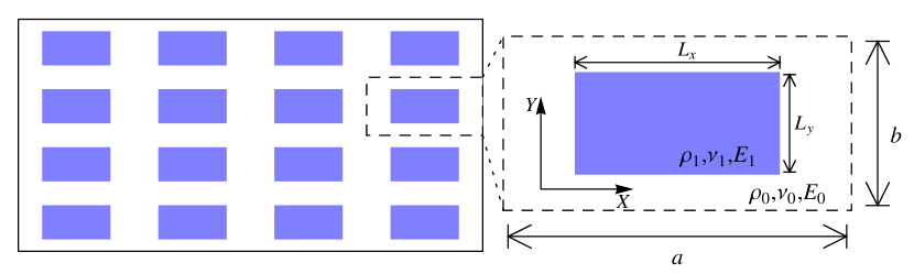
Figure 1: Plane wave expansion method: a rectangular cell of sides $a$ and $b$ is repeated periodically on the plane. Each cell is composed of the plate of interest, in the center of the cell, surrounded by a host material. The elastic properties of the plate of interest have the subindex 1 while the elastic constants of the host material have the subindex 0. The host material mimics the vacuum, in a certain limit, that yields the free–end boundary conditions for the inner plate.

The plane wave expansion method (PWE) refers to a computational technique to solve partial differential equations as an eigenvalue problem [19]. This method is popular among the photonic (phononic) crystal community to obtain the dispersion relation of artificial crystals [20, 21, 22, 23]. In a previous work [16] it was shown that the PWE method can be implemented to solve the out-of-plane Kirchhoff-Love equation for finite systems. As shown below, this numerical method is also useful to solve the in-plane wave equation for finite systems. The main difference between the plane wave expansion method and other numerical methods is that the boundary conditions are not imposed but are rather simulated by introducing a second medium with certain physical properties. A rectangular cell (see Fig. 1) of dimensions $a\times b$ will be used. The plate is located at the center of the cell surrounded by a host material that, for a plate with free ends, mimics the vacuum and, for a plate with clamped ends, mimics an extremely hard medium [16]. The unit cell is repeated periodically in both directions and its mechanical parameters are replaced by a Fourier series truncated at $N$ plane waves. In what follows, the PWE method as used to calculate the in-plane normal modes of plates with free-ends, will be described in detail.

The equations that govern the in-plane motion, in the classical theory of in-plane waves of a thin plate, are [24]

$$\begin{array}[]{l}\displaystyle\frac{\partial N_{x}}{\partial x}+\frac{\partial N_{xy}}{\partial y}=\rho h\frac{\partial^{2}u}{\partial t^{2}},\\ \displaystyle\frac{\partial N_{xy}}{\partial x}+\frac{\partial N_{y}}{\partial y}=\rho h\frac{\partial^{2}v}{\partial t^{2}},\end{array}$$ (1)

where $h$ and $\rho$ are the thickness and density of the plate, respectively. The variables $u(x,y)$ and $v(x,y)$ are the displacements in the $X$ and $Y$ directions, respectively, while the plate stresses are

$$\begin{array}[]{l}\displaystyle N_{x}=C(e_{xx}+\nu e_{yy}),\\ \displaystyle N_{y}=C(e_{yy}+\nu e_{xx}),\\ \displaystyle N_{xy}=C(1-\nu)e_{xy},\end{array}$$ (2)

where $\nu$ is Poisson’s ratio and $C$ is the extensional rigidity given by

$$C=\frac{Eh}{1-\nu^{2}},$$ (3)

with $E$ standing for Young’s modulus. The strain-displacement relations are

$$e_{xx}=\frac{\partial u}{\partial x},\quad e_{yy}=\frac{\partial v}{\partial y}\quad\mathrm{and}\quad e_{xy}=\frac{1}{2}\left(\frac{\partial u}{\partial y}+\frac{\partial v}{\partial x}\right).$$ (4)

Since the mechanical properties of the system of Fig. 1 are periodic, one can assume the following Fourier expansions for the coefficients that appear in Eqs. (1) and (2):

$$C = \sum_{\mathbf{G}}\alpha_{\mathbf{G}}\exp(\mathrm{i}\mathbf{G}\cdot\mathbf{r}),$$ (5)

$$C\nu = \sum_{\mathbf{G}}\beta_{\mathbf{G}}\exp(\mathrm{i}\mathbf{G}\cdot\mathbf{r}),$$ (6)

$$\rho h = \sum_{\mathbf{G}}\eta_{\mathbf{G}}\exp(\mathrm{i}\mathbf{G}\cdot\mathbf{r}).$$ (7)

Here $\mathbf{r}=(x,y)$ is the position and $\mathbf{G}=(G_{x},G_{y})=2\pi(p/a,q/b)$ is a vector of the reciprocal lattice with $p$ and $q$ integers. The displacements $u$ and $v$ are also periodic and can be written in terms of Fourier series as

$$u = \exp(\mathrm{i}\mathbf{k}\cdot\mathbf{r}-\mathrm{i}\omega t)\sum_{\mathbf{G}}\phi_{\mathbf{G}}\exp(\mathrm{i}\mathbf{G}\cdot\mathbf{r}),$$ (8)

$$v = \exp(\mathrm{i}\mathbf{k}\cdot\mathbf{r}-\mathrm{i}\omega t)\sum_{\mathbf{G}}\psi_{\mathbf{G}}\exp(\mathrm{i}\mathbf{G}\cdot\mathbf{r}),$$ (9)

where $\mathbf{k}=(k_{x},k_{y})$ is the wave vector and $\omega$ the angular frequency.

Inserting the expansions (5) to (9) in Eqs. (1) one gets, for each $\mathbf{G}$,

$$\sum_{\mathbf{G}^{\prime}}\mathds{M}_{xx}(\mathbf{G},\mathbf{G}^{\prime})\phi_{\mathbf{G}^{\prime}}+\mathds{M}_{xy}(\mathbf{G},\mathbf{G}^{\prime})\psi_{\mathbf{G}^{\prime}}=\omega^{2}\sum_{\mathbf{G}^{\prime}}\eta_{\mathbf{G}-\mathbf{G}^{\prime}}\phi_{\mathbf{G}^{\prime}},$$ (10)

$$\sum_{\mathbf{G}^{\prime}}\mathds{M}_{yx}(\mathbf{G},\mathbf{G}^{\prime})\phi_{\mathbf{G}^{\prime}}+\mathds{M}_{yy}(\mathbf{G},\mathbf{G}^{\prime})\psi_{\mathbf{G}^{\prime}}=\omega^{2}\sum_{\mathbf{G}^{\prime}}\eta_{\mathbf{G}-\mathbf{G}^{\prime}}\psi_{\mathbf{G}^{\prime}},$$ (11)

where

$$\mathds{M}_{xx}(\mathbf{G},\mathbf{G}^{\prime})=\frac{1}{2}(\alpha_{\mathbf{G}-\mathbf{G}^{\prime}}-\beta_{\mathbf{G}-\mathbf{G}^{\prime}})(k_{y}+G^{\prime}_{y})(k_{y}+G_{y})+\alpha_{\mathbf{G}-\mathbf{G}^{\prime}}(k_{x}+G^{\prime}_{x})(k_{x}+G_{x}),$$ (12)

$$\mathds{M}_{xy}(\mathbf{G},\mathbf{G}^{\prime})=\frac{1}{2}(\alpha_{\mathbf{G}-\mathbf{G}^{\prime}}-\beta_{\mathbf{G}-\mathbf{G}^{\prime}})(k_{x}+G^{\prime}_{x})(k_{y}+G_{y})+\beta_{\mathbf{G}-\mathbf{G}^{\prime}}(k_{x}+G_{x})(k_{y}+G^{\prime}_{y}),$$ (13)

$$\mathds{M}_{yx}(\mathbf{G},\mathbf{G}^{\prime})=\frac{1}{2}(\alpha_{\mathbf{G}-\mathbf{G}^{\prime}}-\beta_{\mathbf{G}-\mathbf{G}^{\prime}})(k_{x}+G_{x})(k_{y}+G^{\prime}_{y})+\beta_{\mathbf{G}-\mathbf{G}^{\prime}}(k_{x}+G^{\prime}_{x})(k_{y}+G_{y}),$$ (14)

and

$$\mathds{M}_{yy}(\mathbf{G},\mathbf{G}^{\prime})=\frac{1}{2}(\alpha_{\mathbf{G}-\mathbf{G}^{\prime}}-\beta_{\mathbf{G}-\mathbf{G}^{\prime}})(k_{x}+G^{\prime}_{x})(k_{x}+G_{x})+\alpha_{\mathbf{G}-\mathbf{G}^{\prime}}(k_{y}+G^{\prime}_{y})(k_{y}+G_{y}).$$ (15)

Eqs. (10) and (11) can be written in matrix form as a generalized eigenvalue equation with an infinite number of columns and rows

$$\left(\begin{array}[]{cc}\mathds{M}_{xx}&\mathds{M}_{xy}\\ \mathds{M}_{yx}&\mathds{M}_{yy}\end{array}\right)\left(\begin{array}[]{c}\phi\\ \psi\end{array}\right)=\omega^{2}\left(\begin{array}[]{cc}\mathds{N}&0\\ 0&\mathds{N}\end{array}\right)\left(\begin{array}[]{c}\phi\\ \psi\end{array}\right),$$ (16)

with $\phi$ and $\psi$ vectors with entries $\phi_{\mathbf{G}^{\prime}}$ and $\psi_{\mathbf{G}^{\prime}}$, respectively, and

$$\mathds{N(\mathbf{G},\mathbf{G}^{\prime})}=\eta_{\mathbf{G}-\mathbf{G}^{\prime}}.$$ (17)

The Fourier coefficients of Eqs. (5) to (7) can be calculated analytically for regular shaped plates, such as the plate of Fig. 1. Plates with irregular shape can also be calculated but in this case the Fourier coefficients should be obtained numerically. The free or clamped boundary conditions can be obtained by defining a host material with $\rho_{0}\rightarrow 0$ or $\rho_{0}\rightarrow\infty$ [16], respectively. Although the generalized eigenvalue equation (16) includes an infinite number of terms, in the numerical calculations the series were truncated to large partial sums. In Fig. 2 some eigenvalues for a rectangular plate with free-ends, as a function of the of the number of plane waves, are plotted. It can be observed that $15\times 15$ plane waves are enough to get stable results at low frequencies but $25\times 25$ plane waves are needed to obtain similar results at high frequencies.

In Tables 1 and 2 the dimensionless normal-mode frequencies of in-plane vibrations of a plate of different aspect ratios with free (F-F-F-F) and clamped (C-C-C-C) ends, respectively, are shown. The results of the PWE method show a very good agreement with the results available in the literature [2, 3, 5, 7] with a difference less than 1.5%. This shows that the PWE method can be used to calculate the normal-mode vibrations of in-plane waves.

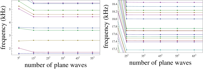
Figure 2: Convergence of the plane wave expansion method for the lower normal modes (left panel) and for higher frequencies (right panel). The results correspond to a plate of $1474$ mm $\times$ $355$ mm.

Table 1: Dimensionless normal-mode frequencies $\Omega=\omega L_{x}\sqrt{\rho(1-\nu^{2})/E}$ for the in-plane vibrations of a rectangular plate with different aspect ratios ($L_{x}/L_{y}$) and completely free (F-F-F-F) boundary conditions.

		aspect ratio $L_{x}/L_{y}=1$								aspect ratio $L_{x}/L_{y}=2$
		PWE		Gorman I			Du and Bardell			PWE		Gorman I			Du and Bardell
Mode		$\Omega$		$\Omega$	%Diff.		$\Omega$	%Diff.		$\Omega$		$\Omega$	%Diff.		$\Omega$	%Diff.
21		2.321		2.320	20.043		2.321	20.000		1.958		1.956	20.112		1.954	20.205
22		2.474		2.472	20.081		2.472	20.081		2.963		2.960	20.101		2.961	20.068
23		2.474		2.472	20.081		2.472	20.081		3.270		3.268	20.061		3.267	20.092
24		2.631		2.628	20.114		2.628	20.114		4.728		4.726	20.042		4.726	20.042
25		2.990		2.988	20.067		2.987	20.100		4.786		4.784	20.042		4.784	20.042
26		3.454		3.452	20.058		3.452	20.058		5.208		5.208	20.000		5.205	20.058
27		3.724		3.724	20.000					5.259		5.258	20.019
28		3.724		3.724	20.000					5.369		5.370	-0.019
29		4.305		4.306	-0.023					6.150		6.148	20.033
10		4.970		4.970	20.000					6.448
11		4.970		4.970	20.000					6.597		6.596	20.015
12		5.047		5.046	20.020					6.750
13		5.257		5.258	-0.019					6.858		6.856	20.029
14		5.288		5.286	20.038					7.452
15		6.044								7.944		7.948	-0.050
16		6.100		6.100	0.000					8.546
17		6.100		6.100	0.000					8.667

• The results obtained with the plane wave expansion method (PWE) are compared with other methods. Gorman I, Du and Bardell results are taken from Refs. [2],  [3] and [7], respectively.

Table 2: Dimensionless normal-mode frequencies $\Omega=\omega L_{x}\sqrt{\rho(1-\nu^{2})/E}$ for the in-plane vibrations of a rectangular plate with different aspect ratios ($L_{x}/L_{y}$) and completely clamped (C-C-C-C) boundary conditions.

		aspect ratio $L_{x}/L_{y}=1$								aspect ratio $L_{x}/L_{y}=2$
		PWE		Gorman II			Du and Bardell			PWE		Gorman II			Du and Bardell
Mode		$\Omega$		$\Omega$	%Diff.		$\Omega$	%Diff.		$\Omega$		$\Omega$	%Diff.		$\Omega$	%Diff.
21		3.551		3.555	-0.113		3.555	-0.113		4.794		4.789	20.104		4.789	20.104
22		3.551		3.555	-0.113		3.555	-0.113		6.348		6.379	-0.486		6.379	-0.486
23		4.241		4.235	20.142		4.235	20.142		6.703		6.712	-0.134		6.712	-0.134
24		5.187		5.185	20.039		5.185	20.039		7.101		7.049	20.738		7.049	20.738
25		5.846		5.859	-0.222		5.859	-0.222		7.650		7.608	20.552		7.608	20.552
26		5.949		5.894	20.933		5.895	20.916		8.180		8.140	20.491		8.140	20.491
27		5.949		5.894	20.933					8.987		8.998	-0.122
28		6.659		6.708	-0.730					9.535		9.515	20.210
29		7.104								9.861
10		7.104								10.640
11		7.280		7.281	-0.014					11.260		11.250	20.089
12		7.572		7.597	-0.329					11.700		11.570	21.124
13		7.865		7.800	20.833					11.900		11.740	21.363
14		8.610								12.200
15		8.610								12.430
16		8.698		8.718	-0.229					13.000
17		8.738								13.020		12.930	20.696

• The results obtained with the plane wave expansion method (PWE) are compared with other methods. Gorman II, Du and Bardell results are taken from Refs. [5],  [3] and [7], respectively.

3 Experimental setup to measure in-plane waves

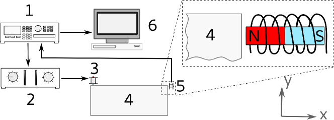
Figure 3: Block diagram of the experimental setup. The vector network analyzer or VNA (1) sends a sinusoidal signal to the power amplifier (2). The amplified signal is sent to the EMAT exciter (3) which produces a mechanical vibration in the aluminum plate (4). The vibrations of the plate are measured by the EMAT detector (5). The measured signal by the EMAT is sent back to the VNA. The experimental data are finally collected in the computer (6) via diskette, serial port or GPIB.

To measure the in-plane normal-mode frequencies for the rectangular plate with free-ends, acoustic resonant spectroscopy (ARS) [25] is used. The experimental setup, shown in Fig. 3, consists of a vector network analyzer (VNA, Anritsu MS4630B); a high fidelity power amplifier (Cerwin-Vega CV900) and two electromagnetic-acoustic transducers (EMATs). The harmonic signal of frequency $f$, generated by the VNA, is sent to the power amplifier whose output is taken by the EMAT exciter. This transducer produces mechanical waves in the plate without mechanical contact. The EMAT detector measures the response of the plate in another location. The signal of this EMAT is registered directly by the VNA which yields the response of the plate at the frequency $f$. The frequency is changed to $f+\Delta f$, with $(\Delta f)/f\ll 1$. The response, as a function of the frequency, is then obtained and the peaks on it will correspond to the resonant frequencies of the plate.

The in-plane resonances of the plate are excited and detected selectively when using electromagnetic-acoustic transducers which consist of coils and magnets in particular configurations (see below). Since the transducers operate through eddy currents, they have to be located in the vicinity of a paramagnetic metal. Let us briefly recall the principles of operation of the EMATs; a detailed explanation of the operation of these transducers is given in Refs. [25, 26]. The EMAT, as an exciter, operates in the following way:

1. A harmonic current, of frequency $f$, passes through the EMAT’s coil; this generates a magnetic field $B(t)$ that varies in time with the same frequency $f$.

2. Due to Faraday’s law of induction, on any circuit of the paramagnetic material which is close to the EMAT’s coil, local eddy currents are generated; these currents are also harmonic.

3. The eddy currents, induced on the paramagnetic metal, interact with the EMAT’s magnet through the Lorentz force.

4. The effect of the Lorenz force on the metal will become a mechanical vibration which travels along the plate.

The EMATs are also invertible, i.e. they can detect the vibrations of a paramagnetic metal. The electromagnetic-acoustic transducer, as a detector, operates in this way:

1. There will be a change of magnetic flux in the loops inside a vibrating paramagnetic metal when the EMAT’s permanent magnet is near it.

2. The change of flux, by Faraday’s law, will produce eddy currents in the metal; these currents oscillate with the frequency $f$ of the vibrating metal.

3. The eddy currents will generate their own alternating magnetic field, which flows through the surface enclosed by the EMAT’s coil. This variable flux will induce on the EMAT’s coil an electromotive force measured by the VNA.

4 Comparison between theory and experiment

In Fig. 3 the configuration of the EMATs used to excite and detect the in-plane vibrations is shown. In this configuration the dipole moment axis of both the EMAT’s coil and permanent magnet coincide and can be considered as the EMAT’s axis; the axis of the exciter is parallel to the Y-axis while the axis of the detector is parallel to the X-axis. To decrease the possibility of missing resonances, i.e. to avoid measuring on a nodal line, the EMATs were located at the corners of the plate on the long side, where it is expected that the wave amplitude will have a maximum due to the free-ends. All the results presented in this section were obtained with this arrangement of EMATs. The main advantage of using the electromagnetic-acoustic transducers, in the configuration of Fig. 3, is that they are highly selective to in-plane vibrations. This result is very important since the measurement of in-plane vibrations is a difficult task.

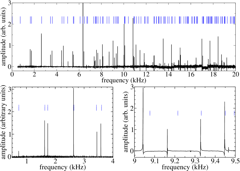
Figure 4: Upper panel: DC to 20 kHz spectrum of a rectangular aluminum plate obtained with the setup of Fig. 3. The EMATs excite and detect selectively in-plane vibrations. The vertical lines correspond to the theoretical predictions obtained with the plane wave expansion method. In the lower panels amplifications, of the spectrum at low and intermediate frequencies, are given.

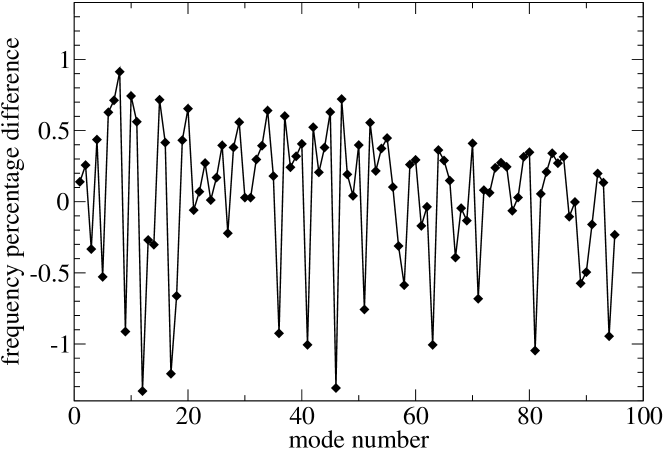
Figure 5: Percentage difference between the experimental and theoretical normal-mode frequencies as a function of the normal mode number.

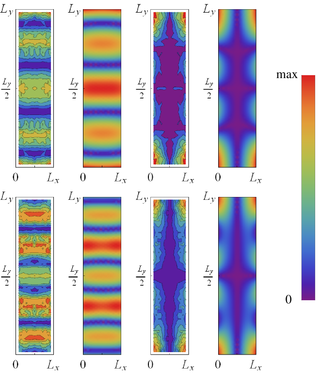
Figure 6: Theoretical and experimental wave amplitudes (absolute value) of the in-plane normal modes of the rectangular aluminum plate of $1474$ mm $\times$ $355$ mm $\times$ $6.35$ mm. The upper and lower parts correspond to modes 4 and 7 of Table 3, respectively. The first and second columns correspond to the EMAT measurement and PWE prediction of $u$, respectively; the third and fourth columns correspond to the EMAT measurement and PWE prediction of $v$, respectively. To avoid spurious border effects, the experimental wave amplitudes were not measured close to the boundary. On the right, the scale is shown.

The spectrum of a rectangular aluminum plate of $1474$ mm $\times$ $355$ mm and thickness $6.35$ mm, measured with the setup of Fig. 3, is given in Table 3 and plotted in Fig. 4. Something worthy to remark, as it can be seen in the lower panels of this figure, is that only in-plane resonances are observed. The theoretical prediction, obtained with the plane wave expansion method, using the best fit elastic constants of aluminum ($E=71.1$ GPa and $\nu=0.36$) and the measured density $\rho=2708$ kg/m³, is also given in Table 3 and plotted in Fig. 4. The agreement is excellent at low frequencies and, remarkably, also at high frequencies (see lower panels of this figure). The difference between the experiment and the theoretical predictions was also quantified and is plotted, as a function of the normal mode number, in Fig. 5. One can observe in this figure that the difference is always less than 1.4%, a very reliable value for more than 90 normal modes.

Table 3: In-plane normal-mode frequencies of a rectangular aluminum plate of $1474$ mm $\times$ $355$ mm $\times$ $6.35$ mm with free ends (F-F-F-F) measured with acoustic resonant spectroscopy (ARS) and calculated with the plane wave expansion method (PWE).

Mode	ARS	PWE	Diff.	Mode	ARS	PWE	Diff.	Mode	ARS	PWE	Diff.
	(Hz)	(Hz)	(%)		(Hz)	(Hz)	(%)		(Hz)	(Hz)	(%)
21	731	730.0	$-0.14$	33	10015	10054.4	$0.39$	65	14910	14953.2	$0.29$
22	1632	1636.2	$0.26$	34	10035	10099.3	$0.64$	66	14938	14960.2	$0.15$
23	1740	1734.2	$-0.33$	35	10094	10112.2	$0.18$	67	15053	14994.0	$-0.39$
24	2634	2645.5	$0.44$	36	10496	10398.9	$-0.92$	68	15094	15087.1	$-0.05$
25	3445	3426.8	$-0.53$	37	10827	10892.2	$0.60$	69	15387	15366.5	$-0.13$
26	3580	3602.5	$0.63$	38	10886	10912.4	$0.24$	70	15485	15548.5	$0.41$
27	4434	4465.6	$0.71$	39	10939	10973.9	$0.32$	71	15674	15567.1	$-0.68$
28	4598	4640.0	$0.91$	40	11098	11143.1	$0.41$	72	15695	15707.7	$0.08$
29	5017	4971.2	$-0.91$	41	11455	11339.7	$-1.01$	73	15721	15730.9	$0.06$
10	5435	5475.4	$0.74$	42	11465	11525.0	$0.52$	74	15726	15763.5	$0.24$
11	5497	5527.9	$0.56$	43	11825	11849.4	$0.21$	75	16009	16052.9	$0.27$
12	6167	6084.9	$-1.33$	44	11859	11904.2	$0.38$	76	16105	16144.5	$0.25$
13	6350	6332.9	$-0.27$	45	12005	12080.7	$0.63$	77	16317	16306.6	$-0.06$
14	6353	6333.8	$-0.30$	46	12339	12177.4	$-1.31$	78	16323	16327.8	$0.03$
15	6435	6481.1	$0.72$	47	12605	12695.9	$0.72$	79	16429	16480.8	$0.32$
16	6660	6687.7	$0.42$	48	12705	12729.4	$0.19$	80	16490	16547.3	$0.35$
17	6839	6756.3	$-1.21$	49	12732	12737.3	$0.04$	81	16782	16606.3	$-1.05$
18	7352	7303.3	$-0.66$	50	12844	12895.1	$0.40$	82	17003	17012.4	$0.06$
19	7405	7437.0	$0.43$	51	13015	12916.4	$-0.76$	83	17054	17089.7	$0.21$
20	7449	7497.7	$0.65$	52	13028	13100.4	$0.56$	84	17078	17136.2	$0.34$
21	7561	7556.5	$-0.06$	53	13095	13123.3	$0.22$	85	17100	17146.3	$0.27$
22	7681	7686.4	$0.07$	54	13185	13234.3	$0.37$	86	17348	17402.6	$0.31$
23	7877	7898.4	$0.27$	55	13300	13359.5	$0.45$	87	17515	17496.5	$-0.11$
24	8094	8094.9	$0.01$	56	13541	13554.9	$0.10$	88	17575	17574.6	$-0.00$
25	8138	8151.8	$0.17$	57	13675	13632.4	$-0.31$	89	17682	17580.5	$-0.57$
26	8457	8490.5	$0.40$	58	13800	13719.1	$-0.59$	90	17723	17635.3	$-0.49$
27	8692	8672.7	$-0.22$	59	13886	13922.2	$0.26$	91	17763	17734.6	$-0.16$
28	9042	9076.5	$0.38$	60	14007	14048.2	$0.29$	92	17766	17801.2	$0.20$
29	9163	9214.2	$0.56$	61	14281	14256.7	$-0.17$	93	17832	17855.9	$0.13$
30	9328	9330.7	$0.03$	62	14339	14333.9	$-0.04$	94	18070	17899.1	$-0.95$
31	9447	9449.7	$0.03$	63	14482	14336.2	$-1.01$	95	18171	18128.7	$-0.23$
32	9466	9494.1	$0.30$	64	14515	14567.7	$0.36$

The measurement of the components $u(x,y)$ and $v(x,y)$ of the in-plane normal-mode wave amplitudes is performed as follows. The in-plane vibrations of the aluminum plate are generated using an EMAT located at one end of the plate in the configuration of Fig. 3. This device is controlled by the VNA, which sends a signal sweeped around the resonant frequency of the wave amplitude to be measured. As it is well known, plotting the norm and phase of the response gives a circle in the complex plane; the radius of the circle is proportional to the wave amplitude. Measurements were carried out on a quarter of the plate in a rectangular grid. The EMAT measures the acceleration in the direction of the coil axis [27]. The wave amplitude is then measured using an EMAT located over the plate; the dipole axis of the magnet’s EMAT is perpendicular to the X-Y plane while the coil axis is aligned along the X or Y direction to measure the deformation $u$ or $v$, respectively. To obtain the wave amplitude on the full plate, the measured data were reflected on the two axes of symmetry of the system. In Fig. 6 some normal-mode wave amplitudes are given and compared with those calculated with the plane wave expansion method; a very good agreement is obtained.

5 Conclusions

The in-plane vibrations of a rectangular aluminum plate, with free ends, have been studied both theoretically and experimentally. The experiments were performed using a vector network analyzer and electromagnetic-acoustic transducers. For the theoretical calculations, the plane wave expansion method, applied to the classical theory of in-plane waves, was used. The plane wave expansion method was first tested by comparing its results with other numerical methods with free and clamped boundary conditions. For 95 normal modes, within the range of DC-20 kHz, the agreement between theory and experiment is excellent since the difference is less than 1.4 percent. Some normal-mode wave amplitudes were measured and compared with the theoretical predictions; very good agreement was obtained. Thus, both the plane wave expansion method and the experimental setup based on electromagnetic-acoustic transducers could be very useful to study in-plane vibrations of thin plates with other shapes.

6 Acknowledgments

This work was partially supported by PAPIIT DGAPA-UNAM under project IN111311. AAL and JAFV were supported by a scholarship from CONACYT; AAL was partially supported by CONACYT under project 79613. Part of this work was written at the Universidad Politécnica de Valencia. We would like to thank Profs. A. L. Salas-Brito, J. Sánchez-Dehesa and S. Ilanko for invaluable comments.

References

- [1] K. Hyde, J.Y. Chang, C. Bacca, J.A. Wickert, Parameter studies for plane stress in-plane vibration of rectangular plates, Journal of Sound and Vibration 247 (2001) 471–487.
- [2] D.J. Gorman, Free in-plane vibration analysis of rectangular plates by the method of superposition, Journal of Sound and Vibration 272 (2004) 831–851.
- [3] J. Du, W.L. Li, G. Jin, T. Yang, Z. Liu, An analytical method for the in-plane vibration analysis of rectangular plates with elastically restrained edges, Journal of Sound and Vibration 306 (2007) 908–927
- [4] D. Larsson, In-plane Modal Testing of a Free Isotropic Rectangular Plate, Experimental Mechanics, 37 (1997) 339–343.
- [5] D.J. Gorman, Accurate analytical type solutions for the free in-plane vibration of clamped and simply supported rectangular plates, Journal of Sound and Vibration 276 (2004) 311–333.
- [6] K. F. Graff, Wave Motion in Elastic Solids, Dover, New York, 1991.
- [7] N.S. Bardell, R.S. Langley, J.M. Dunsdon, On the free in-plane vibration of isotropic rectangular plates, Journal of Sound and Vibration 191 (1996) 459–467.
- [8] B. Liu, Y. Xing, Exact solutions for free in-plane vibrations of rectangular plates, Acta Mechanica Solida Sinica, 24 (2011) 556–567.
- [9] L. Dozio, Free in-plane vibration analysis of rectangular plates with arbitrary elastic boundaries, Mechanics Research Communications 37 (2010) 627–635.
- [10] D.J. Gorman, Free in-plane vibration analysis of rectangular plates with elastic support normal to the boundaries, Journal of Sound and Vibration 285 (2005) 941–966.
- [11] D.J. Gorman, Exact solutions for the free in-plane vibration of rectangular plates with two opposite edges simply supported, Journal of Sound and Vibration 294 (2006) 131–161.
- [12] C.H. Huang, C.C. Ma, Experimental and numerical investigations of resonant vibration characteristics for piezoceramic plates, Journal of the Acoustical Society of America 109 (2001) 2780–2788.
- [13] K. Schaadt, G. Simon, C. Ellegaard, Ultrasound resonances in a rectangular plate described by random matrices, Physica Scripta T90 (2001) 231–237.
- [14] F.J. Nieves, F. Gascon, A. Bayon, Natural frequencies and mode shapes of flexural vibration of plates: laser-interferometry detection and solutions by Ritz’s method, Journal of Sound and Vibration 278 (2004) 637–655.
- [15] C.C. Ma, H.Y. Lin, Experimental measurements on transverse vibration characteristics of piezoceramic rectangular plates by optical methods, Journal of Sound and Vibration 286 (2005) 587–600.
- [16] B. Manzanares-Martínez, J. Flores, L. Gutiérrez, R.A. Méndez-Sánchez, G. Monsivais, A. Morales, F. Ramos-Mendieta, Flexural vibrations of a rectangular plate for the lower normal modes, Journal of Sound and Vibration 329 (2010) 5105–5115.
- [17] Y.F. Xu, W.D. Zhu, Operational modal analysis of a rectangular plate using non-contact excitation and measurement, Journal of Sound and Vibration 332 (2013) 4927–4939.
- [18] J.P. Monchalin, J.D. Aussel, R. Heon, C.K. Jen, A. Boundreault, R. Bernier, Measurement of in-plane and out-of- plane ultrasonic displacements by optical heterodyne interferometry, Journal of Nondestructive Evaluation 8 (1989) 121–132.
- [19] P. Griffin, P. Nagel and R. D. Koshel, The plane-wave expansion method, Journal of Mathematical Physics 15 (1974) 1913–1917.
- [20] Y. Cao, Z. Hou, Y. Liu, Convergence problem of plane-wave expansion method for phononic crystals, Physics Letters A 327 (2004) 247–253.
- [21] Z. Hou, B.M. Assouar, Modeling of Lamb wave propagation in plate with two-dimensional phononic crystal layer coated on uniform substrate using plane-wave-expansion method, Physics Letters A 372 (2008) 2091–2097.
- [22] A.A. Kutsenko, A.L.Shuvalov, A.N.Norris, Converging bounds for the effective shear speed in 2D phononic crystals, Journal of Elasticity 13 (2013) 179–191.
- [23] B. Manzanares-Martínez, F. Ramos-Mendieta, A. Baltazar, Ultrasonic elastic modes in solid bars: An application of the plane wave expansion method, Journal of the Acoustical Society of America 127 (2010) 3503–3510.
- [24] Yi-Yuan Yu, Vibrations of Elastic Plates, Springer-Verlag, New York, 1996.
- [25] J.A. Franco-Villafañe, E. Flores-Olmedo, G. Báez, O. Gandarilla-Carrillo and R.A. Méndez-Sánchez, Acoustic resonance spectroscopy for the advanced undergraduate laboratory, European Journal of Physics 33 (2012) 1761–1769.
- [26] A. Morales, L. Gutiérrez, J. Flores, Improved eddy current driver-detector for elastic vibrations, American Journal of Physics 69 (2001) 517–522.
- [27] A. Díaz-de-Anda, J. Flores, L. Gutiérrez, R.A. Méndez-Sánchez, G. Monsivais and A. Morales, Experimental study of the Timoshenko beam theory predictions, Journal of Sound and Vibration 331 (2012) 5732–5744.