GBLA – Gröbner Basis Linear Algebra Package

Abstract

This is a system paper about a new GPLv2 open source C library GBLA implementing and improving the idea [8] of Faugère and Lachartre (GB reduction). We further exploit underlying structures in matrices generated during Gröbner basis computations in algorithms like F4 or F5 taking advantage of block patterns by using a special data structure called multilines. Moreover, we discuss a new order of operations for the reduction process. In various different experimental results we show that GBLA performs better than GB reduction or Magma in sequential computations (up to $40\%$ faster) and scales much better than GB reduction for a higher number of cores: On $32$ cores we reach a scaling of up to $26$. GBLA is up to $7$ times faster than GB reduction. Further, we compare different parallel schedulers GBLA can be used with. We also developed a new advanced storage format that exploits the fact that our matrices are coming from Gröbner basis computations, shrinking storage by a factor of up to $4$. A huge database of our matrices is freely available with GBLA.

1 Introduction

In [12, 8], Faugère and Lachartre presented a specialized linear algebra for Gröbner basis computation (GB reduction). The benefit of their approach is due to the very special structure the corresponding matrices have. Using algorithms like F4 the tasks of searching for reducers and reducing the input elements are isolated. In the so-called symbolic preprocessing (see [7]) all possible reducers for all terms of a predefined subset of currently available S-polynomials are collected. Out of this data a matrix $M$ is generated whose rows correspond to the coefficients of the polynomials whereas the columns represent all appearing monomials sorted by the given monomial order on the polynomial ring. New elements for the ongoing Gröbner basis computation are computed via Gaussian elimination of $M$, i.e. the reduction process of several S-polynomials at once. $M$ always has a structure like presented in Figure 1, where black dots correspond to nonzero coefficients of the associated polynomials. Faugère and Lachartre’s idea is to take advantage of $M$’s nearly in triangular shape, already before starting the reduction process.

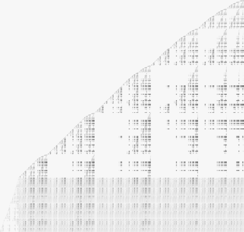
Figure 1: F4 Matrix of degree $6$ for homogeneous Katsura-12

This is a system paper introducing in detail our new open source plain C parallel library GBLA. This library includes efficient implementations not only of the GB reduction but also new algorithmic improvements. Here we present new ways of exploiting the underlying structure of the matrices, introducing new matrix storage formats and various attempts to improve the reduction process, especially for parallel computations. We discuss different experimental results showing the benefits of our new attempt.

The paper is structured as follows: In Section 2 we give an overview of the structure of our library. Section 3 discusses the special matrix structure and presents a new efficient storage format. This is important for testing and benchmarking purposes. We also recall the general process used for reducing these matrices. In Section 4 we first review the main steps of the GB reduction. Afterwards we propose improvements to the sequential algorithm by further exploiting patterns in the matrices. This is implemented in our new library by specialized data structures and a rearrangement of the order of steps of the GB reduction. Section 5 is dedicated to ideas for efficient parallelization of our library that also takes into account the improvements discussed beforehand. In Section 6 we show GBLA’s efficiency by giving experimental results comparing it to several other specialized linear algebra implementations for Gröbner basis computations.

2 Library & Matrices

Our library is called GBLA (Gröbner basis linear algebra) and is the first plain C open source package available for specialized linear algebra in Gröbner basis-like computations. It is based on a first C++ implementation of Fayssal Martani in LELA, which is a fork of LinBox [6] and which is no longer actively developed.

The sources of our library are hosted at: http://hpac.imag.fr/gbla/. Under this website a database of our input matrices in different formats (see Section 3) is available as well as the routines for converting matrices in our special format.

The general structure of the library is presented in Table 1.

Input can come from files on disk or the standard input. The latter is especially useful because we can use a pipe form zcat and never uncompress the matrices to the disk. Uncompressed, our library of matrices would reprensent hundreds of gigabytes of data.

GBLA supports the following data representations:

1. The code is optimized for prime fields $\mathbb{F}_{p}$ with $p<2^{16}$ using SIMD vectorization [3] and storing coefficients as uint16.

2. The library also supports a cofficient representation using float such that we can use the better optimized SIMD instructions for floating point arithmetic. $32$-bit floating points can be used for exact computations over $\mathbb{F}_{p}$ with $p<2^{23}$.

3. There is also a version for $32$-bit field characteristic using uint32 data types that needs further optimization.

Folder	Files	Description
src	types.*	general data types
	matrix.*	matrix and multiline vector types; conversion routines for sparse, hybrid, block, multiline matrices
	mapping.*	splicing of input matrix (Step $1$ in GB reduction); different routines for usual block and multiline vector submatrix representations
	elimination.*	elimination routines including Steps $2-4$ of GB reduction as well as adjusted routines for new order of operations (see Section 4.3)
cli	io.*	input and output routines
	gbla.*	main routines for GB reduction
tools	dump_matrix.*	routines for dumping matrices; especially towards MatrixMarket or Magma formats
	converter.c	converting matrices from format 1 to format 2 (see Section 3.2)

Table 1: Description of GBLA’s structure

Note that whereas it is true that vectorization in CPUs is faster for floating point arithmetic compared to exact one we show in Section 6 that for $16$-bit computations memory usage can become a bottleneck: Representing data via uint16 can make matrices manageable that are not feasible when using float data type.

For parallelization GBLA is based on OpenMP. Current versions of XKAAPI can interpret OpenMP macros, so one can also easily use GBLA with XKAAPI as scheduler.

In order to assure cache locality we use blocks, all of them of dimension $256\times 256$ by default. The user has the freedom to set this to any power of $2$, but in all of our experiments the preset size is advantageous due to L1 cache size limitations.

At the moment we have two different types of implementations of the usual GB reduction (see Section 1) and the new order of operations for rank computations (see Section 4.3) each:

1. The first type of implementations is completely based on the multiline data structure, denoted GBLA-v0.1.

2. The second type is nearly always faster and denoted GBLA-v0.2 in this paper. There we use multilines only in a very specific block situation where we can nearly guarantee in advance that they give a speedup due to cache locality. Otherwise we use usual sparse resp. dense row representations that are advantageous when sorting rows by pivots.

Note that GBLA-v0.2 is able to reduce matrices that GBLA-v0.1 cannot due to it’s smaller memory footprint not introducing too many zeroes in multilines (see also Section 6).

3 File formats and FL matrices

Input matrices in the GB reduction have some nearly-triangular structure and patterns in the coefficients that we take advantage of. We describe GB matrices and an efficient way to store them.

3.1 Description of FL matrices

Matrices coming from Gröbner basis computations represent a set of polynomials in a polynomial ring w.r.t. to some given monomial order. This order sorts the columns of the matrix, each column represents a monomial. Each row represents a polynomial whereas the entries are just the coefficients of the polynomial for the corresponding monomial in the appropriate column. Due to this, GB matrices are sparse. We can assume that the matrix has been sorted by weight (number of non zero elements) with row $0$ the heaviest. Pivoting the rows corresponds to reordering of the polynomials; permuting non pivot columns is allowed once before the GB reduction and re-done after the elimination steps.

The first non zero element on each row is a $1$ (each polynomial is monic), and this element will be called pivoting candidate. Every such pivoting candidate lies below the main diagonal. Columns whose last non zero element is not a pivoting candidate can be permuted in order to separate them from the pivot ones.

Now, the first $n_{\text{piv}}$ columns contain pivoting candidates, called pivot columns. Among the pivoting candidates of a given column, one row is selected, the pivot row. This selection tries to keep $A$ (a $n_{\text{piv}}\times n_{\text{piv}}$ matrix) as sparse as possible.

3.2 Compressed binary format

In standard Matrix Market file format, GB matrices are huge (hundreds of Gb) and slow to read. We compress them to a CSR-like (Compressed Storage Row) format and store them in binary format (i.e. streams of bytes rather than a text file). We propose two different formats , see Table 2. The files consist in consecutive sequences of elements of type size repeated length times.

Format 1			Format 2
Size	Length	Data	Size	Length	Data
			uint32_t	1	b
uint32_t	1	m	uint32_t	1	m
uint32_t	1	n	uint32_t	1	n
uint32_t	1	p	uint64_t	1	p
uint64_t	1	nnz	uint64_t	1	nnz
uint16_t	nnz	data	uint32_t	m	rows
uint32_t	nnz	cols	uint32_t	m	polmap
uint32_t	m	rows	uint64_t	1	k
			uint64_t	k	colid
			uint32_t	1	pnb
			uint64_t	1	pnnz
			uint32_t	pnb	prow
			xinty_t	pnnz	pdata

Table 2: Structure of the binary matrix formats.

In Format 1, m, n, p, nnz resp. represent the number of rows, columns, the modulo and the number of non zeros in the sparse matrix. rows[i] represents the length of the $i$^th row. If $j$ is the sum $\texttt{row[0]}+\dots+\texttt{row[i-1]}$, then on row $i$, there is an element at column cols[j+r] with value data[j+r] for all $r$ in $\left\{0,\dots,\texttt{row[i]}-1\right\}$.

In Format 2, we separate the location of the non zero entries and the data. We store the data of the polynomials separately since there is redundancy: many lines will be of the form $m_{i}f_{j}$ where $m_{i}$ is some monomial and $f_{j}$ is a polynomial in the intermediate Gröbner basis. Hence the coefficients in all lines of this type correspond to the same polynomial $f_{j}$ and represent the same data, only the location on the basis changes. We allow to store the data on different machine types to adapt to the size of $p$. Data is blocked, so we utilize the fact that several non zero elements on a row may be adjacents, allowing compression of their consecutive column numbers. In this format matrices must have less than $2^{31}$ rows.

First, the lowest 3 bits of the first element b represent the value of x and y in xinty_t, namely $b=\texttt{u\ OR\ (v << 1)}$ where $u$ is $1$ iff the type is signed and $y$ corresponds to a type on $8\cdot 2^{v}$ bits (for instance $\overline{011}^{2}=\texttt{1 OR (1 << 1)}$ represents uint16_t type. On the highest bits a mask is used to store a file format version.

The $i\textsuperscript{th}$ row has rows[i] elements. We prefer storing the row length since it fits on $32$ bits while pointers (the accumulated row length) would fit on $64$ bits.

We compress the column indices: If $s>1$ several non zero elements are consecutive on a row and if $f$ is the first one, then we store $f$ $s$ in the format. If $s=1$ then we use a mask and store f AND (1 << 31). Here we lose a bit for the number of rows.

So far, we have stored the locations of the non zero elements. The polynomial data on a row is stored in pdata in the following fashion. $\texttt{prow}[i]$ gives the $i\textsuperscript{th}$ polynomial number of elements (its support). There are pnb polynomials. $j=\texttt{polmap[i]}$ maps the polynomial number $j$ on row $i$. The polynomial data is laid out contiguously in pdata, polynomial $0$ finishes at pdata+prow[0], polynomial $1$ finishes at pdata+prow[0]+prow[1], and so on.

In table 3 we show the raw size (in gigabits) of a few sparse matrices in their binary format, compressed with gzip (default options) and the time it takes (in seconds). Compressing format 2 yields an $8$ time improvement on the original uncompressed binary format 1 storage and over $4$ times better than compressed format 1, in a much shorter time. The compressed format 2 is hence much faster to load and it makes it easier to perform tests on.

Matrix	Format 1			Format 2
	Size	Compressed	Time	Size	Compressed	Time
F4-kat14-mat9	2.3Gb	1.2Gb	230s	0.74Gb	0.29Gb	66s
F5-kat17-mat10	43Gb	24Gb	4419s	12Gb	5.3Gb	883s

Table 3: Storage and time efficiency of the new format

4 Echelon Forms for Gröbner Bases

In this section we present new developments in the implementation of the GB reduction that can be found in our library (see Section 2). Section 4.2 presents ideas to exploit the structure of the input GB matrix $M$ further with dedicated data structures, and Section 4.3 gives an alternative ordering of the steps of the GB reduction if a non-reduced row echelon form of $M$ is sufficient.

4.1 The reduction by Faugère and Lachartre

There are $4$ main steps in the GB reduction:

1. The input matrix $M$ already reveals a lot of its pivots even before the Gaussian elimination starts. For exploiting this fact we rearrange the rows and the columns: we reach a cutting of $M$ into $\begin{pmatrix}A&B\\ C&D\end{pmatrix}$. After this rearrangement one can see $4$ different parts of $M$: A very sparse, upper triangular unit matrix on the top left ($A$) representing the already known pivots. A denser, but still sparse top right part ($B$) of the same number of rows. Moreover, there are two bottom parts, a left one which is still rather sparse ($C$) and a right one, which tends to be denser ($D$). Whereas $A$ represents already known leading terms in the intermediate Gröbner basis, $D$ corresponds to the new polynomials added to the basis after the reduction step. If $M$ is of dimensions $m\times n$ and if $n_{\text{piv}}$ denotes the number of known pivots the characteristics of the four splices of $M$ are given in Table 4.

   Splice	Dimensions	approx. density
   $A$	$n_{\text{piv}}\times n_{\text{piv}}$	$<2\%$
   $B$	$n_{\text{piv}}\times(n-n_{\text{piv}})$	$12\%$
   $C$	$(m-n_{\text{piv}})\times n_{\text{piv}}$	$15\%$
   $D$	$(m-n_{\text{piv}}\times n-n_{\text{piv}})$	$35\%$

   Table 4: Characteristics of matrix splices in GB reduction

   In general, $n_{\text{piv}}\gg m-n_{\text{piv}}$ and $n_{\text{piv}}\gg n-n_{\text{piv}}$.

2. In the second step of the GB reduction the known pivot rows are reduced with each other, we perform an TRSM. Algebraically, this is equivalent to computing $B\leftarrow A^{-1}\times B$. $A$ is invertible due to being upper triangular with $1$s on the diagonal. From an implementational point of view one only reads $A$ and writes to $B$. After this step, we receive a representation of $M$ in the format $\begin{pmatrix}\text{Id}_{n_{\text{piv}}}&A^{-1}\times B\\ C&D\end{pmatrix}$.

3. In the third step, we reduce $C$ to zero using the identity matrix $\text{Id}_{n_{\text{piv}}}$ performing AXPY. Doing this we also have to carry out the corresponding operations induced by $B$ on $D$. We get

   $$\begin{pmatrix}\text{Id}_{n_{\text{piv}}}&A^{-1}\times B\\ 0&D-C\times\left(A^{-1}\times B\right)\end{pmatrix}.$$

4. The fourth step now reveals the data we are searching for: Via computing a Gaussian Elimination on $D-C\times\left(A^{-1}\times B\right)$ we receive new pivots reaching an upper triangular matrix $D^{\prime}$. Those new pivots correspond to new leading terms in our Gröbner basis, thus the corresponding rows represent new polynomials to be added to the basis. On the other hand, rows reducing to zero correspond to zero reductions in the Gröbner basis computation.

5. As the last step we rearrange the columns of the echelon form of $M$ and read off polynomials whose monomials are sorted correctly w.r.t. the monomial order.

If one is interested in a reduced row echelon form of $M$ we have to perform the GB reduction a second time, but only on the right part $\begin{pmatrix}A^{-1}\times B\\ D^{\prime}\end{pmatrix}$. From the Gröbner basis point of view a fully reduced row echelon form has the advantage that also the multiples of polynomials already in the basis, i.e. elements representing the rows $\begin{pmatrix}A&B\end{pmatrix}$ are reduced. Thus, reusing them in later reduction steps of the Gröbner basis computation can be beneficial; we refer to Section $2.4$ in [7] discussing the Simplify procedure.

4.2 Multiline data structure

As already seen in Section 4.1, matrices coming from Gröbner basis computations are structured in a way that can be exploited for a specialized Gaussian Elimination. Furthermore, there are even more patterns in such matrices that we use in order to speed up the computations. In Figure 1 we can see that the nonzero entries are, in general, grouped in blocks. In other words, if there is a nonzero element $m_{i,j}$ at position $j$ in row $i$ then also $m_{i,j+1}$ (horizontal pattern) and $m_{i+1,j}$ (vertical pattern) tend to be nonzero, too. This fact can be used, for example, to optimize the AXPY resp. TRSM computations in the second step of the GB reduction as illustrated in Figure 2: Assuming that $a_{i,j}$ and $a_{i+1,j}$ are both not zero (horizontal pattern), element $b_{i,\ell}$ is updated by both nonzero elements $b_{k,\ell}$ and $b_{k+1,\ell}$ (vertical pattern). Whereas the horizontal patterns are canonically taken care ofstoring blocks row-wise, we have to pack the vertical pattern in a dedicated data structure.

Figure 2: Exploiting horizontal and vertical patterns in the TRSM step.

Definition 1

An $n$-multiline vector ml is a data structure consisting of two vectors in a sparse representation:

1. A position vector pos of column indices such that at each index at least one of $n$ rows of elements has a nonzero element.

2. A value vector val of entries of $M$. The entries of all $n$ rows in column $\text{\tt pos}[i]$ are stored consecutively, afterwards the $n$ entries at position $\text{\tt pos}[i+1]$ are stored. Note that val may have zero elements.

If pos has a length $\ell$, val has length $n\cdot\ell$. In this situation we say that ml has length $\ell$. For a $2$-multiline vector we use the shorthand notation multiline vector.

Example 1

Consider the following two rows:

$\begin{array}[]{rcccccccccc}r_{1}&=&[&2&0&0&1&0&0&5&],\\ r_{2}&=&[&1&7&0&0&0&1&0&].\end{array}$

A sparse representation is given by $v_{i}$ (values) and $p_{i}$ (positions):

$\begin{array}[]{rcccccccccccccc}v_{1}&=&[&2&1&5&]&&v_{2}&=&[&1&7&1&],\\ p_{1}&=&[&0&3&6&]&&p_{2}&=&[&0&1&5&].\\ \end{array}$

A $2$-multiline vector representation of $r_{1}$ and $r_{2}$ is given by

$\begin{array}[]{lccccccccccccccc}\text{\tt ml}.\text{\tt val}&=&[&2&1&\color[rgb]{0.765625,0.07421875,0.07421875}{0}&7&1&\color[rgb]{0.765625,0.07421875,0.07421875}{0}&\color[rgb]{0.765625,0.07421875,0.07421875}{0}&1&5&\color[rgb]{0.765625,0.07421875,0.07421875}{0}&],\\ \text{\tt ml}.\text{\tt pos}&=&[&0&1&3&5&6&].\\ \end{array}$

Four zero values are added to $\text{\tt ml}.\text{\tt val}$, two from $r_{1}$ and $r_{2}$ resp. We do not add column $2$ since there both, $r_{1}$ and $r_{2}$ have zero entries.

Multiline vectors are especially useful when performing AXPY. In the following we use multiline vectors to illustrate the reduction of two temporarily dense rows $\text{dense}_{1}$ and $\text{dense}_{2}$ with one multiline vector ml of length $\ell$. For the entries in $\text{\tt ml}.\text{\tt val}$ two situations are possible: Either there is only one of $\text{\tt ml}.\text{\tt val}[2i]$ and $\text{\tt ml}.\text{\tt val}[2i+1]$ nonzero, or both are nonzero. Due to the vertical pattern of GB matrices very often both entries are nonzero. We can perform a specialized ${\tt AXPY}$ operation on $\text{dense}_{1}$ and $\text{dense}_{2}$ with scalars $\lambda_{1,1},\lambda_{1,2}$ coming from column $j$ and $\lambda_{2,1},\lambda_{2,2}$ from column $j+1$ where $j$ is the loop step in the corresponding ${\tt TRSM}$ opteration:

1:$\text{dense}_{1}$, $\text{dense}_{2}$, $\lambda_{1,1}$, $\lambda_{1,2}$, $\lambda_{2,1}$, $\lambda_{2,2}$, ml.

2:$v_{1}$, $v_{2}$, $i$, $k$

3:for $\left(i=0;\;i<\ell;\;i\leftarrow i+1\right)$ do

4:    $k\leftarrow\text{\tt ml}.\text{\tt pos}[i]$

5:    $v_{1}\leftarrow\text{\tt ml}.\text{\tt val}[2i]$

6:    $v_{2}\leftarrow\text{\tt ml}.\text{\tt val}[2i+1]$

7:    $\text{dense}_{1}[k]\leftarrow\lambda_{1,1}v_{1}+\lambda_{1,2}v_{2}$

8:    $\text{dense}_{2}[k]\leftarrow\lambda_{2,1}v_{1}+\lambda_{2,2}v_{2}$

Algorithm 1 ${\tt AXPY}$ of two dense rows of length $\ell$ with a multiline vector.

The benefit of Algorithm 1 is clear: We perform $4$ reductions (each dense row is reduced by two rows) in one step. On the other hand, if the horizontal pattern does not lead to two successive nonzero entries (for example if $a_{i,j+1}$ is zero in Figure 2), then Algorithm 1 would not use $\text{\tt ml}.\text{\tt val}[2i+1]$. This would introduce an disadvantage due to using only every other element of $\text{\tt ml}.\text{\tt val}$. In our implementation we take care of this situation and have a specialized ${\tt AXPY}$ implementation for that. Still, we are performing two reductions (each dense row is reduced by one row) in one step.

Assuming general $n$-multiline vectors the problem of introducing useless operations on zero elements appears. For multiline vectors, i.e. $n=2$, we can perform lightweight tests before the actual loop to ensure execution only on nonzero $\lambda_{1,1},\lambda_{1,2}$ (for single ${\tt AXPY}$) resp. $\lambda_{1,1},\lambda_{1,2},\lambda_{2,1},\lambda_{2,2}$ (for Algorithm 1). For general $n$ we cannot predict every possible configuration of the $n^{2}$ scalars $\lambda_{1,1},\ldots,\lambda_{n,n}$. Moreover, for $n$-multiline vectors the memory overhead can get problematic, too. For $n=2$ we can lose at most $\text{\tt sizeof}(\text{entry})$ bytes per column index, but for arbitrary $n$ this increases to $(n-1)\cdot\text{\tt sizeof}(\text{entry})$ bytes. All in all, we note the following fact that is also based on practical experimental results.

Remark 1

Based on cache efficiency as well as memory overhead due to adding zero entries to the val vector $2$-multiline vector data structures are the most efficient.

As already mentioned in [10], representing the matrices $A$, $B$, $C$ and $D$ in blocks has several benefits: Firstly, we can pack data in small blocks that fit into cache and thus we increase spatial and temporal locality. Secondly, separating the data into column blocks we can perform operations on $B$ and $D$ rather naturally in parallel. Thus we are combining the multiline vector data structure with a block representation in our implementation. In the following, presented pseudo code is independent of the corresponding row resp. block representation, standard row representation is used. Multiline representations impede the readability of the algorithms, if there is an impact on switching to multilines, we point this out in the text.

Using multilines is useful in situations where we can predict horizontal and vertical patterns with a high probability, in order to see advantages and drawbacks we have two different implementations, GBLA-v0.1 and GBLA-v0.2, which use multilines in different ways (see also Section 2).

4.3 New order of operations

If the number of initially known pivots (i.e. the number of rows of $A$ and $B$) is large compared to the number of rows of $C$ and $D$, then most work of the GB reduction is spent in reducing $A$, the TRSM step $A^{-1}B$. For the Gröbner basis the new information for updating the basis is strictly in $D$. Thus, if we are not required to compute a reduced echelon form of the input matrix $M$, but if we are only interested in the reduction of $D$ resp. the rank of $M$ we can omit the TRSM step. Whereas in [10] the original GB reduction removes nonzero entries above ($A^{-1}B$) and below (deleting $C$) the known pivots, it is enough to reduce elements below the pivots.

Thus, after splicing the input matrix $M$ of dimension $m\times n$ we can directly reduce $C$ with $A$ while reflecting the corresponding operations with $B$ on $D$ with the following steps.

1:submatrices $A\left(n_{\text{piv}}\times n_{\text{piv}}\right)$, $B\left(n_{\text{piv}}\times(n-n_{\text{piv}})\right)$, $C\left((m-n_{\text{piv}})\times n_{\text{piv}}\right)$, $D\left((m-n_{\text{piv}})\times(n-n_{\text{piv}})\right)$.

2:$\text{dense}_{C}$, $\text{dense}_{D}$, $i$, $j$

3:for $\left(i=0;\;i<m-n_{\text{piv}};\;i\leftarrow i+1\right)$ do

4:    $\text{dense}_{C}\leftarrow\textrm{copy\_sparse\_row\_to\_dense}(C[i,*])$

5:    $\text{dense}_{D}\leftarrow\textrm{copy\_sparse\_row\_to\_dense}(D[i,*])$

6:    for $\left(j=0;\;j<n_{\text{piv}};\;j\leftarrow j+1\right)$ do

7:         if $\left(\text{dense}_{C}[j]\neq 0\right)$ then

8:             ${\tt AXPY}\left(\text{dense}_{C},\text{dense}_{C}[j],A[j,*]\right)$

9:             ${\tt AXPY}\left(\text{dense}_{D},\text{dense}_{C}[j],B[j,*]\right)$              

10:    $D[i,*]\leftarrow\textrm{copy\_dense\_row\_to\_sparse}(\text{dense}_{D})$

Algorithm 2 Reduction of $C$ and $D$

Whereas Algorithm 2 describes the idea of reducing $C$ and $D$ from a mathematical point of view, in practice one would want to use a block representation for the data in order to improve cache locality and also parallelization. Strangely, it turned out that this is not optimal for efficient computations: In order for a block representation to make sense one needs to completely reduce all rows resp. multilines in a given block before reducing the next block. That is not a problem for $B$ and $D$ since their blocks do not depend on the columns, but it is disadvantageous for $A$ and $C$. Assuming an operation on a lefthand side block of $C$ due to a reduction from a block from $A$. Any row operation on $C$ must be carried out through all blocks on the right. Even worse, whenever we would try to handle $C$ per row resp. multiline and $D$ per block at the same time this would introduce a lot of writing to $D$. Thus, in our implementation we found the most efficient solution to be the following:

1. Store $A$ and $C$ in multiline representation and $B$ and $D$ in block multiline representation as defined in Section 4.2.

2. Carry out the reduction of $C$ by $A$, but store the corresponding coefficients needed for the reduction of $D$ by $B$ later on.

3. Transform $C$ to block multiline representation $C^{\prime}$.

4. Reduce $D$ by $B$ using thecoefficients stored in $C^{\prime}$.

Thus we have an optimal reduction of $C$ and an optimal reduction of $D$. The only overhead we have to pay for this is the transformation from $C$ to $C^{\prime}$. But copying $C$ into block format is negligible compared to the reduction operations done in $C$ and $D$.

In Section 6 we see that this new order of operations is faster than the standard GB reduction for full rank matrices from F5. The density of the row echelon form of $M$ does not vary too much from $M$’s initial density which leads in less memory footprint.

4.4 Modified structured Gaussian Elimination

Computing the row echelon form of $D$ the original FL Implementation used a sequential structured Gaussian Elimination. Here we use a modified variant that can be easily parallelized.

1:submatrix $D\left((m-n_{\text{piv}})\times(n-n_{\text{piv}})\right)$.

2:$\text{rank}_{D}$, rank of $D$

3:$\text{dense}_{D}$, $i$, $j$

4:$\text{rank}_{D}\leftarrow 0$

5:for $\left(i=0;\;i<m-n_{\text{piv}};\;i\leftarrow i+1\right)$ do

6:    $\text{normalize}(D[i,*])$

7:    $\text{dense}_{D}\leftarrow\textrm{copy\_sparse\_row\_to\_dense}(D[i,*])$

8:    for $\left(j=0;\;j<i-1;\;j\leftarrow j+1\right)$ do

9:         if $\left(\text{head}(\text{dense}_{D})=\text{head}(D[j,*])\right)$ then

10:             ${\tt AXPY}\left(\text{dense}_{D},\text{head}(\text{dense}_{D}),D[j,*]\right)$              

11:    $D[i,*]\leftarrow\textrm{copy\_dense\_row\_to\_sparse}(\text{dense}_{D})$

12:    $\text{normalize}(D[i,*])$

13:    if $\left(\text{not\_empty}(D[i,*])\right)$ then

14:         $\text{rank}_{D}\leftarrow\text{rank}_{D}+1$     

15:return $\text{rank}_{D}$

Algorithm 3 Modified structured Gaussian Elimination of $D$

In Algorithm 3 we do a structured Gaussian Elimination on the rows of $D$. Note that $D$ is not a unitary matrix, so normalization and inversions are required. At the very end the rank of $D$ is returned. The modification lies mainly in the fact that once we have found a new pivot row, we do not sort the list of known pivot rows, but just add the new one. This is due to the usage of multilines in our implementation. Storing two (or more) rows in this packed format it is inefficient to sort pivots by column index. Possibly we would need to open a multiline row and move the second row to another position. For this, all intermediate multiline rows need to be recalculated. Thus we decided to relinquish the sorting at this point of the computation and sort later on when reconstructing the row echelon form of the initial matrix $M$. Note that whereas we use multilines everywhere in GBLA-v0.1, in GBLA-v0.2 (see Section 6) we restrict the usage of multilines to specific block situations and no longer use them for the dense Gaussian Elimination of $D$. Thus we are able to perform a sorting of the pivots.

5 Parallelization

In this section we discuss improvements concerning parallelizing the GB reduction taking the new ideas presented in the last section into account. For this we have experimented with different parallel schedulers such as OpenMP, XKAAPI and pthreads. Moreover, whereas the initial implementation of Faugère and Lachartre used a sequential Gaussian Elimination of $D$ we are now able to use a parallel version of Algorithm 3.

5.1 Parallelization of the modified structured Gaussian Elimination

As already discussed in Section 4.4 we use a modified structured Gaussian Elimination for multilines which omits sorting the list of known pivots, postponed to the reconstruction of the echelon form of the input matrix $M$. In our library GBLA there is also a non-multiline version with sorting, see Section 6 for more information.

Assuming that we have already found $k$ pivots in Algorithm 3, we are able to reduce several rows of index $>k$ in parallel. The $k$ pivots are already in their normalized form, they are readonly, thus we can easily update $D[\ell,*]\leftarrow D[\ell,*]+\sum_{i=0}^{k}\lambda_{i}D[i,*]$for all $k<\ell<m-n_{\text{piv}}$ and corresponding multiples $\lambda_{i}$. Clearly, this introduces some bookkeeping: Whereas in the above situation $D[k+1,*]$ is fully reduced with the $k$ known pivots, the rows $D[k+j,*]$ for $j>1$ are not. Thus we can add $D[k+1,*]$ to the list of known pivots, but not $D[k+j,*]$. We handle this by using a global waiting list $W$ which keeps the rows not fully reduced and the indices of the last pivot row up to which we have already updated the corresponding row. Different threads share a global variable lp: the last known pivot. Each thread performs the following operations:

1. Fetch the next available row $D[j,*]$ which was not updated up to this point or which is already in the waiting list $W$.

2. Reduce it with all pivots not applied until now, up to lp.

3. If $j=\text{\tt lp}+1$, $D[j,*]$ is a new pivot and lp is incremented.

4. If $j\neq\text{\tt lp}+1$, $D[j,*]$ is added to $W$ keeping track that lp is the index of the last row $D[j,*]$ is already reduced with.

Naturally, the above description leaves some freedom for the decision which row to fetch and reduce next in Step 1. We found the following choice to be the most efficient for a wide range of examples: When a thread fetches a row to be further reduced it prefers a row that was already previously reduced. This often leads to a faster recognition of new known pivots in Step 3. Synchronization is needed in Steps 3 and 4, besides this the threads can work independent of each other. We handle the communication between the threads using spin locks whose implementation w.r.t. a given used different parallel scheduler (see Section 5.2) might differ slightly.

Talking about load balancing it can happen that one thread gets stuck in reducing already earlier reduced rows further, whereas other threads fetch pristine rows and fill up $W$ more and more. In order to avoid this we use the following techniques:

• If a thread has just fully reduced a row $r$ and thus adds a new known pivot, this thread prefers to take an already reduced row from $W$ possibly waiting for $r$ to become a known pivot.

• If a thread has added $t$ new rows to $W$ consecutively, it is triggered to further reduce elements from $W$ instead of starting with until now untouched rows from $D$.

For efficiency reasons we do not directly start with the discussed parallel elimination, but we do a sequential elimination on the first $k$ rows resp. multiline rows of $D$. In this way we can avoid high increasing on the waiting list $W$ at the beginning, which would lead to tasks too small to benefit from the available number of cores executing in parallel. Thus $k$ depends on the number of threads used, in practice we found that $k=2\times(\text{number of threads})$ is a good choice. Clearly, the efficiency of this choice depends on how many of the first $k$ rows resp. multiline rows of $D$ reduce to zero in this step. This is not a problem for full rank matrices coming from F5 Gröbner basis computations.

5.2 Different parallel schedulers

We did some research on which parallel schedulers to be used in our library. For this we tested not only well known schedulers like OpenMP [4] and Intel TBB [13] but also XKAAPI [11] and StarPU [1]. We also did experiments with pthreads and own implementations for scheduling. Most of the schedulers have advantages and disadvantages in different situations like depending on sparsity, blocksizes or relying on locking for the structured Gaussian Elimination. Moreover, all those packages are actively developed and further improved, thus we realized different behavoiour for different versions of the same scheduler. In the end we decided to choose OpenMP for the current state of the library.

1. It is in different situations usually not the fastest scheduler, but often tends to be the fastest for the overall computation.

2. Our library should be plain C as much as possible, thus we discarded the usage of Intel TBB which is based on high-level C++ features for optimal usage.

3. Current versions of XKAAPI are able to interpret OpenMP pragmas. Thus one can use our library together with XKAAPI by changing the linker call: instead of libgomp one has to link against libkomp (see also Section 6).

4. Using pthreads natively is error-prone and leads to code that is not portable (it is not trivial to get them work on Windows machines). OpenMP’s locking mechanism boils down to pthreads on UNIX and their pendants on Windows without having to deal with different implementations.

5. StarPU’s performance depends highly on the used data structures. Since the representation of our data is special (see Sections 3 and 4) we need further investigations on how to get data and scheduler playing together efficiently. Moreover, the fact that StarPU can be used for task scheduling even on heterogeneous multicore architectures like CPU/GPU combinations makes it a good candidate for further experiments.

6 Experimental results

Matrix			Rows	Columns	Nonzeros	Density
			$\times 10^{3}$	$\times 10^{3}$	$\times 10^{6}$	%
F4	kat12	mat9	18.8	22.3	17.1	4.07
	kat13	mat2	4.68	6.53	1.45	4.74
		mat3	12.1	14.6	7.78	4.35
		mat5	35.4	38.2	63.7	4.13
		mat9	43.5	49.2	75.3	3.52
	kat14	mat8	100	103	352	3.39
	kat15	mat7	168	178	832	2.77
		mat8	197	210	1,060	2.55
		mat9	228	234	1,521	2.84
	eco14	mat24	105	107	91.1	0.81
	eco16	mat13	157	141	293	1.32
	mr-9-8-8-5	mat7	26.0	34.1	236	26.6
		mat8	22.1	34.6	189	25.5
	rand16-d2-2	mat5	67.1	106	199	2.80
		mat6	146	217	689	2.19
	rand16-d2-3	mat8	587	874	4,328	0.84
		mat9	980	1,428	8,378	0.60
		mat10	1,544	2,199	14,440	0.43
		mat11	2,287	3,226	23,823	0.32
	rand18-d2-9	mat5	430	1,028	1,048	0.24
		mat6	1,212	2,674	3,879	0.12
F5	kat13	mat5	28.4	35.5	26.8	2.66
		mat6	34.5	42.3	35.9	2.46
	kat14	mat7	69.6	84.5	118	2.01
		mat8	81.0	96.9	156	1.98
	kat15	mat7	139	167	383	1.63
		mat8	168	199	507	1.51
		mat9	187	219	640	1.56
		mat10	195	227	725	1.63
	kat16	mat5	83.8	110	139	1.50
		mat6	168	208	485	1.38
		mat9	393	456	2,234	1.25
	cyc10	mat19	192	256	1,182	2.40
		mat20	303	378	2,239	1.95
	cyc10-sym1	mat17	29.8	43.3	114	0.09
	mr-9-10-7	mat3	20.1	74.5	532	35.5
		mat7	88.5	192	4,055	23.8
	rand16-d2-2	mat11	1,368	1,856	15,134	0.60
		mat12	1,806	2,425	22,385	0.51
		mat13	2,310	3,076	31,247	0.44
	rand16-d2-3	mat8	578	871	3,140	0.62
		mat9	973	1,426	6,839	0.49
		mat10	1,532	2,198	13,222	0.39
		mat11	2,286	3,226	23,221	0.31
		mat12	3.266	4,550	37,796	0.25
	rand18-d2-9	mat5	429	1,027	9,65	0.22
		mat7	3,096	6,414	12,594	0.06
		mat11	1,368	1,856	15,135	0.60

Table 5: Some matrix characteristics

The following experiments were performed on http://hpac.imag.fr/ which is a NUMA architecture of 4x8 processors. Each of the 32 non hyper-threaded Intel(R) Xeon(R) CPUs cores clocks at 2.20GHz (maximal turbo frequency on single core 2.60GHz). Each of the 4 nodes has 96Gb of memory, so we have 384Gb of RAM in total. The compiler is gcc-4.9.2. The timings do not include the time spent on reading the files from disk. We state matrix characteristics of our example set in Table 5.

We use various example sets: There are well known benchmarks like Katsura, Eco and Cyclic. Moreover, we use matrices from minrank problems arising in cryptography. Furthermore we have random dense systems randx-d2-y-mat* in x variables, all input polynomials are of degree $2$. Then we deleted y polynomials to achieve higher-dimensional benchmarks. All examples are done over the biggest $16$-bit prime field, $\mathbb{F}_{65521}$. We use the uint16 coefficient representation in GBLA. If not otherwise stated GBLA’s timings are done using OpenMP as parallel scheduler.

6.1 Behaviour on F5 matrices

We show in Table 6 a comparison with Faugère and Lachartre’s FL Implementation from [10] and GBLA. Timings are in seconds, using 1, 16 or 32 threads. This is done for F5 matrices, thus we can use GBLA’s new order of operations (see Section 4.3) to compute a Echelon form and to verify that the matrices have full rank.

Implementation	FL Implementation			GBLA-v0.1			GBLA-v0.2
F5 Matrix / # Threads	1	16	32	1	16	32	1	16	32
kat13-mat5	16.7	2.7	2.3	14.5	2.02	1.87	14.5	1.73	1.61
kat13-mat6	27.3	4.15	4.0	23.9	3.08	2.65	25.9	3.03	2.28
kat14-mat7	139	17.4	16.6	142	13.4	10.6	122	11.2	8.64
kat14-mat8	181	24.95	23.1	177	16.9	12.7	158	14.7	10.5
kat15-mat7	629	61.8	55.6	633	55.1	38.2	553	46.3	30.7
kat16-mat6	1,203	110	83.3	1,147	98.7	69.9	988	73.9	49.0
mr-9-10-7-mat3	591	70.8	71.3	733	57.3	37.9	747	52.8	33.2
mr-9-10-7-mat7	15,787	1,632	1,565	15,416	1,103	793	15,602	1,057	591
cyc10-mat19	7,482	693	492	1,291	135	103	1,030	80.3	62.9
cyc10-mat20	17,853	1,644	1,180	2,589	274	209	2,074	171	152
cyc10-sym1-mat17	11,083	1,982	1,705	2,463	465	405	2,391	275	245
rand16-d2-2-mat11	mem	mem	mem	2,568	946	883	4,553	425	360
rand16-d2-2-mat12	mem	mem	mem	5,751	1,252	1,219	6,758	632	527
rand16-d2-2-mat13	mem	mem	mem	mem	mem	mem	8,435	816	721
rand16-d2-3-mat8	2,084	500	472	2,243	339	282	1,654	144	106
rand16-d2-3-mat9	bug	bug	bug	2,938	827	781	2,308	236	227
rand16-d2-3-mat10	mem	mem	mem	2,528	922	940	4,518	427	372
rand16-d2-3-mat11	mem	mem	mem	mem	mem	mem	11,254	931	696
rand16-d2-3-mat12	mem	mem	mem	mem	mem	mem	15,817	1,369	1,150
rand18-d2-9-mat5	1,469	287	250	350	297	306	340	52.9	50.3
rand18-d2-9-mat7	mem	mem	mem	mem	mem	mem	8,752	1,112	1,098
rand18-d2-9-mat11	bug	bug	bug	2,540	923	882	4,600	415	363

Table 6: GB reduction vs. GBLA (time in seconds)

Usually GBLA-v0.1 is faster on one core than FL Implementation, GBLA-v0.2 is even faster than GBLA-v0.1. Both GBLA implementations have a much better scaling than FL Implementation, where GBLA-v0.2 preforms better than GBLA-v0.1, even scaling rather good for smaller examples, where the overhead of scheduling different threads starts to become a bottleneck. The only example where FL Implementation is faster than GBLA is mr-9-10-7-mat3, a very dense ($35.5\%$) matrix. This good behaviour for FL Implementation might be triggered from the fact that FL Implementation allocates all the memory needed for the computation in advance. Usually the user does not know how much memory the computation might need, so this approach is a bit error-prone. Still, FL Implementation is faster than GBLA only on one core, starting to use several CPU cores the better scaling of GBLA wins (already at $2$ cores the timings are nearly identical). Moreover, for dense matrices like the minrank ones we can see a benefit of the multiline structure, at least for fewer cores. Once the number of cores increases the better scaling of GBLA-v0.2 is favourable.

For cyc10-sym1-mat17 the speedup between $16$ and $32$ is quite small. Due to the applied symmetry the matrix is already nearly reduced, so the scheduling overhead has a higher impact than the gain during reduction for anything greater than $16$ cores.

For the higher-dimensional random examples the row dimension of $C$ and $D$ is very small ($<300$). Our new order of operations (Section 4.3) enables GBLA to reduce matrices the FL Implementation is not able to handle. Even GBLA-v0.2 reaches for rand18-d2-9-mat7 the memory limit of the machine, but it is still able to reduce the matrix. Memory overhead due to multilines hinders GBLA-v0.1 to compute rand16-d2-3-mat11, but is more efficient on rand16-d2-3-mat10 for one core.

6.2 Behaviour on F4 matrices

In Table 7 we compare Magma-2.19 [2] to GBLA. Since there is no F5 implementation in Magma we can only compare matrices coming from F4 computations. Since Magma is closed source we are not able to access the specialized linear algebra for Gröbner basis computations directly. Thus, we are comparing the same problem sets with the same degrees running Magma’s F4 implementation. Note that Magma generates matrices that are, for the same problem and same degree, slightly larger, usually $5$ to $10$%. Note that we use only Magma’s CPU implementation of F4, but not the rather new GPU one. We think that it is not really useful to compare GPU and CPU parallelized code. Furthermore, most of our examples are too big to fit into the RAM of a GPU, so data copying between CPU and GPU might be problematic for an accurate comparison.

Implementation	Magma	GBLA-v0.1			GBLA-v0.2
F4 Matrix / # Threads	1	1	16	32	1	16	32
kat12-mat9	11.2	11.4	1.46	1.60	11.3	1.40	1.40
kat13-mat2	0.94	1.18	0.38	0.61	1.11	0.26	0.33
kat13-mat3	9.33	11.0	1.70	3.10	8.51	1.07	1.13
kat13-mat9	168	165	16.0	11.8	114	9.74	6.83
kat14-mat8	2,747	2,545	207	165	1,338	104	65.8
kat15-mat7	10,345	9,514	742	537	4,198	298	195
kat15-mat8	13,936	12,547	961	604	6,508	470	283
kat15-mat9	24,393	22,247	1,709	1,256	10,923	779	450
eco14-mat24	524	169	22.2	21.9	146	16.2	16.5
eco16-mat13	6,239	1,537	184	176	1,346	104	72.9
mr-9-8-8-5-mat7	1,073	1,080	88.5	57.9	550	41.6	24.7
mr-9-8-8-5-mat8	454	600	48.5	30.3	318	25.6	14.9
rand16-d2-2-mat5	740	778	62.2	40.8	589	43.6	28.6
rand16-d2-2-mat6	4,083	4,092	375	219	3,054	224	133
rand16-d2-3-mat8	55,439	48,008	3,473	2,119	26,533	1,782	1,027
rand16-d2-3-mat9	91,595	65,126	4,869	2,983	39,108	2,614	1,372
rand16-d2-3-mat10	mem	-	9,691	6,223	-	3,820	1,972
rand16-d2-3-mat11	mem	mem	mem	mem	-	5,399	2,385
rand18-d2-9-mat5	2,020	1,892	414	388	630	63.1	61.8
rand18-d2-9-mat6	4,915	6,120	981	941	1,736	220	218

Table 7: Magma vs. GBLA (time in seconds)

For small examples Magma, not splicing the matrices, has an advantage. But already for examples in the range of $10$ seconds GBLA, especially GBLA-v0.2 gets faster on single core. The difference between Magma and GBLA-v0.1 is rather small, whereas GBLA-v0.2 becomes more than twice as fast. Moreover, GBLA-v0.1 and GBLA-v0.2 scale very well on $16$ and $32$ cores. Due to lack of space we do not state timings for the FL Implementation. It behaves in nearly all examples like expected: Due to preallocation of all memory it is very fast on sequential computations (nearly as fast as GBLA-v0.2), but it scales rather bad. For example, for kat14-mat8 FL Implementation runs in $1,571$s, $861$s and $868$s for $1$, $16$ and $32$ cores, respectively. Also note that FL Implementation’s memory consumption is higher than GBLA’s.

For the random, higher dimensional examples Magma cannot reduce matrices starting from rand16-d2-3-mat9 due to the float representation of the matrix entries and resulting higher memory usage on the given machine. For rand16-d2-3-mat11 even GBLA-v0.1 consumes too much memory by using multilines and thus introducing too many zeros (see Section 4.2). Even GBLA-v0.2 comes to the limit of our chosen compute server, but it can still reduce the matrix: At the end of the computation the process consumed $98\%$ of the machine’s RAM.

6.3 Comparing OpenMP (OMP) and XKAAPI (XK)

We compare the different behaviour of the parallel schedulers that can be used in GBLA (see also Section 5.2): The default scheduler in GBLA is OMP, here we use the latest stable version $4.0$. XK can interpret OMP pragmas, too, so we are able to run GBLA with XK by just changing the linker call from libgomp to libkomp. The latest stable version of XK we use is $3.0$. In Table 8 we compare both schedulers on representative benchmarks in GBLA-v0.1 and GBLA-v0.2 on $16$ and $32$ cores. The timings show that in many examples both schedulers are on par. XK tends to be a bit more efficient on $32$ cores, but that is not always the case. F4-kat15-mat8 and F4-kat15-mat9 are cases where XK has problems on $32$ cores for GBLA-v0.1. This comes from the last step, the structured Gaussian Elimination of $D$ where GBLA-v0.1, using multilines, cannot sort the pivots which seems to become a bottleneck for XK’s scheduling. For the same examples in GBLA-v0.2 (now with sorting of pivots) we see that XK is even a bit faster than OMP. All in all, in our setting both schedulers behave nearly equal.

Implementation	GBLA-v0.1				GBLA-v0.2
# Threads	16		32		16		32
Matrix / Scheduler	OMP	XK	OMP	XK	OMP	XK	OMP	XK
F4-kat15-mat8	961	916	604	1,223	470	463	283	277
F4-kat15-mat9	1,709	1,679	1,256	2,122	779	774	450	431
F4-rand16-d2-3-mat8	3,4732	3,447	2,119	1,964	1,782	1,818	1,027	1,017
F4-rand16-d2-3-mat9	6,956	7,073	4,470	3,783	3,214	3,141	1,776	1,785
F5-kat16-mat6	98.7	105	69.9	67.2	73.9	75.3	49.0	49.0
F5-mr-9-10-7-mat3	57.3	59.6	37.9	38.8	52.8	54.8	33.2	34.7
F5-cyc10-mat19	135	140	103	101	80.3	86.7	62.9	60.9
F5-cyc10-mat20	274	292	209	206	171	203	152	141
F5-cyc10-sym1-mat17	465	496	405	406	275	272	245	217

Table 8: OpenMP vs. XKAAPI (time in seconds)

7 Conclusion

We presented the first open-source, plain C library for linear algebra specialized for matrices coming from Gröbner basis computations including various new ideas exploiting underlying structures. This led to more efficient ways of performing the GB reduction and improved parallel scaling. Moreover, the library uses a new compressed file format that enables us to generate matrices not feasible beforehand. Corresponding routines for dumping and converting own matrices are included such that researchers are able to use their own data in our new format in GBLA.

Also the time needed to reduce $D$ during GB reduction is in general very small compared to the overall reduction, we plan to investigate our parallel structured Gaussian elimination implementation in the future. For this we may again copy $D^{\prime}$ first to a different data representation and use external libraries for fast exact linear algebra such as FFLAS-FFPACK [5] in given situations.

References

- [1] C. Augonnet, S. Thibault, R. Namyst, and P.-A. Wacrenier. Starpu: A unified platform for task scheduling on heterogeneous multicore architectures. Concurr. Comput. : Pract. Exper., 23(2):187–198, Feb. 2011.
- [2] Bosma, W., Cannon, J., and Playoust, C. The Magma algebra system. I. The user language. Journal of Symbolic Computation, 24(3-4):235–265, 1997. http://magma.maths.usyd.edu.au/magma/.
- [3] B. Boyer, J.-G. Dumas, P. Giorgi, C. Pernet, and B. Saunders. Elements of design for containers and solutions in the linbox library. In H. Hong and C. Yap, editors, Mathematical Software – ICMS 2014, volume 8592 of Lecture Notes in Computer Science, pages 654–662. Springer Berlin Heidelberg, 2014.
- [4] L. Dagum and R. Menon. Openmp: an industry standard api for shared-memory programming. Computational Science & Engineering, IEEE, 5(1):46–55, 1998.
- [5] J. Dumas, T. Gautier, C. Pernet, and Z. Sultan. Parallel computation of echelon forms. In F. M. A. Silva, I. de Castro Dutra, and V. S. Costa, editors, Euro-Par 2014 Parallel Processing - 20th International Conference, Porto, Portugal, August 25-29, 2014. Proceedings, volume 8632 of Lecture Notes in Computer Science, pages 499–510. Springer, 2014.
- [6] J.-G. Dumas, T. Gautier, M. Giesbrecht, P. Giorgi, B. Hovinen, E. L. Kaltofen, B. D. Saunders, W. J. Turner, and G. Villard. LinBox: A generic library for exact linear algebra. In Proceedings of the 2002 International Congress of Mathematical Software, Beijing, China. World Scientific Pub, Aug. 2002.
- [7] J.-C. Faugère. A new efficient algorithm for computing Gröbner bases (F4). Journal of Pure and Applied Algebra, 139(1–3):61–88, June 1999.
- [8] J.-C. Faugère and S. Lachartre. Parallel Gaussian Elimination for Gröbner bases computations in finite fields. In M. Moreno-Maza and J. L. Roch, editors, Proceedings of the 4th International Workshop on Parallel and Symbolic Computation, PASCO ’10, pages 89–97, New York, NY, USA, July 2010. ACM.
- [9] Faugère, J.-C. and Svartz, J. Gröbner Bases of ideals invariant under a Commutative group : the Non-modular Case. In Proceedings of the 38th international symposium on International symposium on symbolic and algebraic computation, ISSAC ’13, pages 347–354, New York, NY, USA, 2013. ACM.
- [10] J.-C. Faugère and S. Lachartre. Parallel Gaussian Elimination for Gröbner bases computations in finite fields. In M. Moreno-Maza and J. L. Roch, editors, Proceedings of the 4th International Workshop on Parallel and Symbolic Computation, PASCO ’10, pages 89–97, New York, NY, USA, July 2010. ACM.
- [11] T. Gautier, X. Besseron, and L. Pigeon. Kaapi: A thread scheduling runtime system for data flow computations on cluster of multi-processors. In Proceedings of the 2007 International Workshop on Parallel Symbolic Computation, PASCO ’07, pages 15–23, New York, NY, USA, 2007. ACM.
- [12] S. Lachartre. Algèbre linéaire dans la résolution de systèmes polynomiaux Applications en cryptologie. PhD thesis, Université Paris 6, 2008.
- [13] J. Reinders. Intel Threading Building Blocks. O’Reilly & Associates, Inc., Sebastopol, CA, USA, first edition, 2007.