Structured Sparse Regression via Greedy Hard-Thresholding

Prateek Jain
Microsoft Research, India
   Nikhil Rao
Technicolor R & I, Los Altos, CA
   Inderjit Dhillon
University of Texas at Austin
Abstract

Several learning applications require solving high-dimensional regression problems where the relevant features belong to a small number of (overlapping) groups. For very large datasets and under standard sparsity constraints, hard thresholding methods have proven to be extremely efficient, but such methods require NP hard projections when dealing with overlapping groups. In this paper, we show that such NP-hard projections can not only be avoided by appealing to submodular optimization, but such methods come with strong theoretical guarantees even in the presence of poorly conditioned data (i.e. say when two features have correlation 0.99absent0.99\geq 0.99), which existing analyses cannot handle. These methods exhibit an interesting computation-accuracy trade-off and can be extended to significantly harder problems such as sparse overlapping groups. Experiments on both real and synthetic data validate our claims and demonstrate that the proposed methods are orders of magnitude faster than other greedy and convex relaxation techniques for learning with group-structured sparsity.

1 Introduction

High dimensional problems where the regressor belongs to a small number of groups play a critical role in many machine learning and signal processing applications, such as computational biology [9] and multitask learning [14]. In most of these cases, the groups overlap, i.e., the same feature can belong to multiple groups. For example, gene pathways overlap in computational biology applications, and parent-child pairs of wavelet transform coefficients overlap in signal processing applications.

The existing state-of-the-art methods for solving such group sparsity structured regression problems can be categorized into two broad classes: a) convex relaxation based methods , b) iterative hard thresholding (IHT) or greedy methods. In practice, IHT methods tend to be significantly more scalable than the (group-)lasso style methods that solve a convex program. But, these methods require a certain projection operator which in general is NP-hard to compute and often certain simple heuristics are used with relatively weak theoretical guarantees. Moreover, existing guarantees for both classes of methods require relatively restrictive assumptions on the data, like Restricted Isometry Property or variants thereof [2, 8, 18, 14], that are unlikely to hold in most common applications. In fact, even under such settings, the group sparsity based convex programs offer at most polylogarithmic gains over standard sparsity based methods [18].

Concretely, let us consider the following linear model:

𝒚=X𝒘+𝜷,𝒚𝑋superscript𝒘𝜷\bm{y}=X\bm{w}^{*}+\bm{\beta}, (1)

where 𝜷N(0,λ2I)similar-to𝜷𝑁0superscript𝜆2𝐼\bm{\beta}\sim N(0,\lambda^{2}I), Xn×p𝑋superscript𝑛𝑝X\in\mathbb{R}^{n\times p}, each row of X𝑋X is sampled i.i.d. s.t. 𝒙iN(0,Σ)similar-tosubscript𝒙𝑖𝑁0Σ\bm{x}_{i}\sim N(0,\Sigma), 1in1𝑖𝑛1\leq i\leq n, and 𝒘superscript𝒘\bm{w}^{*} is a ksuperscript𝑘k^{*}-group sparse vector i.e. 𝒘superscript𝒘\bm{w}^{*} can be expressed in terms of only ksuperscript𝑘k^{*} groups, Gj[p]subscript𝐺𝑗delimited-[]𝑝G_{j}\subseteq[p].

The existing analyses for both convex as well as hard thresholding based methods require κ=σ1/σpc𝜅subscript𝜎1subscript𝜎𝑝𝑐\kappa=\sigma_{1}/\sigma_{p}\leq c, where c𝑐c is an absolute constant (like say 333) and σisubscript𝜎𝑖\sigma_{i} is the i𝑖i-th largest eigenvalue of ΣΣ\Sigma. This is a significantly restrictive assumption as it requires all the features to be nearly independent of each other. For example, if features 111 and 222 have correlation more than say .99.99.99 then the restriction on κ𝜅\kappa required by the existing results do not hold.

Moreover, in this setting (i.e., when κ=O(1)𝜅𝑂1\kappa=O(1)), the number of samples required to exactly recover 𝒘superscript𝒘\bm{w}^{*} (with λ=0𝜆0\lambda=0) is given by: n=Ω(s+klogM)𝑛Ω𝑠superscript𝑘𝑀n=\Omega(s+k^{*}\log M) [18], where s𝑠s is the maximum support size of a union of ksuperscript𝑘k^{*} groups and M𝑀M is the number of groups. In contrast, if one were to directly use sparse regression techniques (by ignoring group sparsity altogether) then the number of samples is given by n=Ω(slogp)𝑛Ω𝑠𝑝n=\Omega(s\log p). Hence, even in the restricted setting of κ=O(1)𝜅𝑂1\kappa=O(1), group-sparse regression improves upon the standard sparse regression only by logarithmic factors.

Greedy, Iterative Hard Thresholding (IHT) methods have been considered for group sparse regression problems, but they involve NP-hard projections onto the constraint set [3]. While this can be circumvented using approximate operations, the guarantees they provide are along the same lines as the ones that exist for convex methods.

In this paper, we show that IHT schemes with approximate projections for the group sparsity problem yield much stronger guarantees. Specifically, our result holds for arbitrarily large κ𝜅\kappa, and arbitrary group structures. In particular, using IHT with greedy projections, we show that n=Ω((slog1ϵ+κ2klogM)log1ϵ)𝑛Ω𝑠1italic-ϵsuperscript𝜅2superscript𝑘𝑀1italic-ϵn=\Omega\left((s\log\frac{1}{\epsilon}+\kappa^{2}k^{*}\log M)\log\frac{1}{\epsilon}\right) samples suffice to recover ϵitalic-ϵ\epsilon-approximatation to 𝒘superscript𝒘\bm{w}^{*} when λ=0𝜆0\lambda=0. On the other hand, IHT for standard sparse regression [11] requires n=Ω(κ2slogp)𝑛Ωsuperscript𝜅2𝑠𝑝n=\Omega(\kappa^{2}s\log p). Moreover, for general noise variance λ2superscript𝜆2\lambda^{2}, our method recovers 𝒘^^𝒘\hat{\bm{w}} s.t. 𝒘^𝒘2ϵ+λκs+κ2klogMnnorm^𝒘superscript𝒘2italic-ϵ𝜆𝜅𝑠superscript𝜅2superscript𝑘𝑀𝑛\|\hat{\bm{w}}-\bm{w}^{*}\|\leq 2\epsilon+\lambda\cdot\kappa\sqrt{\frac{s+\kappa^{2}k^{*}\log M}{n}}. On the other hand, the existing state-of-the-art results for IHT for group sparsity [5] guarantees 𝒘^𝒘λs+klogMnorm^𝒘superscript𝒘𝜆𝑠superscript𝑘𝑀\|\hat{\bm{w}}-\bm{w}^{*}\|\leq\lambda\cdot\sqrt{s+k^{*}\log M} for κ3𝜅3\kappa\leq 3, i.e., 𝒘^^𝒘\hat{\bm{w}} is not a consistent estimator of 𝒘superscript𝒘\bm{w}^{*} even for small condition number κ𝜅\kappa.

Our analysis is based on an extension of the sparse regression result by [11] that requires exact projections. However, a critical challenge in the case of overlapping groups is the projection onto the set of group-sparse vectors is NP-hard in general. To alleviate this issue, we use the connection between submodularity and overlapping group projections and a greedy selection based projection is at least good enough. The main contribution of this work is to carefully use the greedy projection based procedure along with hard thresholding iterates to guarantee the convergence to the global optima as long as enough i.i.d. data points are generated from model (1).

Moreover, the simplicity of our hard thresholding operator allows us to easily extend it to more complicated sparsity structures. In particular, we show that the methods we propose can be generalized to the sparse overlapping group setting, and to hierarchies of (overlapping) groups.

We also provide extensive experiments on both real and synthetic datasets that show that our methods are not only faster than several other approaches, but are also accurate despite performing approximate projections. Indeed, even for poorly-conditioned data, IHT methods are an order of magnitude faster than other greedy and convex methods. We also observe a similar phenomenon when dealing with sparse overlapping groups.

1.1 Related Work

Several papers, notably [6] and references therein, have studied convergence properties of IHT methods for sparse signal recovery under standard RIP conditions. [11] generalized the method to settings where RIP does not hold, and also to the low rank matrix recovery setting. [24] used a similar analysis to obtain results for nonlinear models. However, these techniques apply only to cases where exact projections can be performed onto the constraint set. Forward greedy selection schemes for sparse [22, 10] and group sparse [20] constrained programs have been considered previously, where a single group is added at each iteration. The authors in [2] propose a variant of CoSaMP to solve problems that are of interest to us, and again, these methods require exact projections.

Several works have studied approximate projections in the context of IHT [4, 19, 7, 13]. However, these results require that the data satisfies RIP-style conditions which typically do not hold in real-world regression problems. Moreover, these analyses do not guarantee a consistent estimate of the optimal regressor when the measurements have zero-mean random noise. In contrast, we provide results under a more general RSC/RSS condition, which is weaker [23] and provide crisp rates for the error bounds when the noise in measurements is random.

2 Group Iterative Hard Thresholding for Overlapping Groups

In this section, we formally set up the group sparsity constrained optimization problem, and then briefly present the IHT algorithm for the same. Suppose we are given a set of M𝑀M groups that can arbitrarily overlap 𝒢={G1,,GM}𝒢subscript𝐺1subscript𝐺𝑀\mathcal{G}=\{G_{1},\ldots,G_{M}\}, where Gi[p]subscript𝐺𝑖delimited-[]𝑝G_{i}\subseteq[p]. Also, let i=1MGi={1,2,,p}superscriptsubscript𝑖1𝑀subscript𝐺𝑖12𝑝\cup_{i=1}^{M}G_{i}=\{1,2,\ldots,p\}. We let 𝒘norm𝒘\|\bm{w}\| denote the Euclidean norm of 𝒘𝒘\bm{w}, and supp(𝒘)supp𝒘\mbox{supp}(\bm{w}) denotes the support of 𝒘𝒘\bm{w}. For any vector 𝒘p𝒘superscript𝑝\bm{w}\in\mathbb{R}^{p}, [9] defined the overlapping group norm as

𝒘𝒢:=infi=1M𝒂Gis.t.i=1M𝒂Gi=𝒘,supp(𝒂Gi)Giformulae-sequenceassignsuperscriptnorm𝒘𝒢infimumsuperscriptsubscript𝑖1𝑀normsubscript𝒂subscript𝐺𝑖s.t.formulae-sequencesuperscriptsubscript𝑖1𝑀subscript𝒂subscript𝐺𝑖𝒘suppsubscript𝒂subscript𝐺𝑖subscript𝐺𝑖\|\bm{w}\|^{\mathcal{G}}:=\inf\sum_{i=1}^{M}\|\bm{a}_{G_{i}}\|\ \ \textbf{s.t.}\leavevmode\nobreak\ \ \sum_{i=1}^{M}\bm{a}_{G_{i}}=\bm{w},\ \mbox{supp}(\bm{a}_{G_{i}})\subseteq G_{i} (2)

We also introduce the notion of “group-support” of a vector and its group-0subscript0\ell_{0} pseudo-norm:

Gsupp(𝒘):={is.t.𝒂Gi>0},𝒘0𝒢:=infi=1M𝟙{𝒂Gi>0},\operatorname{G-supp}(\bm{w}):=\{i\ s.t.\ \|\bm{a}_{G_{i}}\|>0\},\qquad\|\bm{w}\|_{0}^{\mathcal{G}}:=\inf\sum_{i=1}^{M}\mathds{1}\{\|\bm{a}_{G_{i}}\|>0\}, (3)

where 𝒂Gisubscript𝒂subscript𝐺𝑖\bm{a}_{G_{i}} satisfies the constraints of (2). 𝟙{}1\mathds{1}\{\cdot\} is the indicator function, taking the value 111 if the condition is satisfied, and 0 otherwise. For a set of groups G𝐺G, supp(G)={Gi,iG}supp𝐺subscript𝐺𝑖𝑖𝐺\operatorname{supp}(G)=\{G_{i},\ i\in G\}. Similarly, Gsupp(S)=Gsupp(𝒘S)Gsupp𝑆Gsuppsubscript𝒘𝑆\operatorname{G-supp}(S)=\operatorname{G-supp}(\bm{w}_{S}).

Suppose we are given a function f:p:𝑓superscript𝑝f:\mathbb{R}^{p}\rightarrow\mathbb{R} and M𝑀M groups 𝒢={G1,,GM}𝒢subscript𝐺1subscript𝐺𝑀\mathcal{G}=\{G_{1},\ldots,G_{M}\}. The goal is to solve the following group sparsity structured problem (GS-Opt):

GS-Opt:min𝒘f(𝒘)s.t.𝒘0𝒢kGS-Opt:subscript𝒘𝑓𝒘s.t.subscriptsuperscriptnorm𝒘𝒢0𝑘\textbf{GS-Opt:}\qquad\qquad\min_{\bm{w}}f(\bm{w})\leavevmode\nobreak\ \ \textbf{s.t.}\leavevmode\nobreak\ \ \|\bm{w}\|^{\mathcal{G}}_{0}\leq k (4)

f𝑓f can be thought of as a loss function over the training data, for instance, logistic or least squares loss. In the high dimensional setting, problems of the form (4) are somewhat ill posed and are NP-hard in general. Hence, additional assumptions on the loss function (f𝑓f) are warranted to guarantee a reasonable solution. Here, we focus on problems where f𝑓f satisfies the restricted strong convexity and smoothness conditions:

Definition 2.1 (RSC/RSS).

The function f:p:𝑓superscript𝑝f:\mathbb{R}^{p}\rightarrow\mathbb{R} satisfies the restricted strong convexity (RSC) and restricted strong smoothness (RSS) of order k𝑘k, if the following holds:

αkIH(𝒘)LkI,precedes-or-equalssubscript𝛼𝑘𝐼𝐻𝒘precedes-or-equalssubscript𝐿𝑘𝐼\alpha_{k}I\preceq H(\bm{w})\preceq L_{k}I,

where H(𝐰)𝐻𝐰H(\bm{w}) is the Hessian of f𝑓f at any 𝐰p𝐰superscript𝑝\bm{w}\in\mathbb{R}^{p} s.t. 𝐰0𝒢ksubscriptsuperscriptnorm𝐰𝒢0𝑘\|\bm{w}\|^{\mathcal{G}}_{0}\leq k.

Note that the goal of our algorithms/analysis would be to solve the problem for arbitrary αk>0subscript𝛼𝑘0\alpha_{k}>0 and Lk<subscript𝐿𝑘L_{k}<\infty. In contrast, adapting existing IHT results to this setting lead to results that allow Lk/αksubscript𝐿𝑘subscript𝛼𝑘L_{k}/\alpha_{k}less than a constant (like say 333).

We are especially interested in the linear model described in (1), and in recovering 𝒘superscript𝒘\bm{w}^{\star} consistently (i.e. recover 𝒘superscript𝒘\bm{w}^{\star} exactly as n𝑛n\rightarrow\infty). To this end, we look to solve the following (non convex) constrained least squares problem

GS-LS:𝒘^=argmin𝒘f(𝒘):=12n𝒚𝑿𝒘2s.t.𝒘0𝒢kformulae-sequenceGS-LS:^𝒘subscript𝒘𝑓𝒘assign12𝑛superscriptnorm𝒚𝑿𝒘2s.t.subscriptsuperscriptnorm𝒘𝒢0𝑘\textbf{GS-LS:}\qquad\qquad\hat{\bm{w}}=\arg\min_{\bm{w}}f(\bm{w}):=\frac{1}{2n}\|\bm{y}-\bm{X}\bm{w}\|^{2}\leavevmode\nobreak\ \ \textbf{s.t.}\leavevmode\nobreak\ \ \|\bm{w}\|^{\mathcal{G}}_{0}\leq k (5)

with kk𝑘superscript𝑘k\geq k^{*} being a positive, user defined integer 111typically chosen via cross-validation. In this paper, we propose to solve (5) using an Iterative Hard Thresholding (IHT) scheme. IHT methods iteratively take a gradient descent step, and then project the resulting vector (𝒈)𝒈(\bm{g}) on to the (non-convex) constraint set of group sparse vectos, i.e.,

𝒘=Pk𝒢(𝒈)=argmin𝒘𝒘𝒈2s.t𝒘0𝒢kformulae-sequencesubscript𝒘superscriptsubscript𝑃𝑘𝒢𝒈subscript𝒘superscriptnorm𝒘𝒈2s.tsuperscriptsubscriptnorm𝒘0𝒢𝑘\bm{w}_{*}=P_{k}^{\mathcal{G}}(\bm{g})=\arg\min_{\bm{w}}\|\bm{w}-\bm{g}\|^{2}\leavevmode\nobreak\ \ \textbf{s.t}\leavevmode\nobreak\ \ \|\bm{w}\|_{0}^{\mathcal{G}}\leq k (6)

Computing the gradient is easy and hence the complexity of the overall algorithm heavily depends on the complexity of performing the aforementioned projection. Algorithm 1 details the IHT procedure for the group sparsity problem (4). Throughout the paper we consider the same high-level procedure, but consider different projection operators P^k𝒢(𝒈)superscriptsubscript^𝑃𝑘𝒢𝒈\widehat{P}_{k}^{\mathcal{G}}(\bm{g}) for different settings of the problem.

Algorithm 1 IHT for Group-sparsity
1:  Input : data 𝒚,𝑿𝒚𝑿\bm{y},\bm{X}, parameter k𝑘k, iterations T𝑇T, step size η𝜂\eta
2:  Initialize: t=0,𝒘0pformulae-sequence𝑡0superscript𝒘0superscript𝑝t=0,\leavevmode\nobreak\ \ \bm{w}^{0}\in\mathbb{R}^{p} a k𝑘k-group sparse vector
3:  for t = 1, 2, …, T do
4:     𝒈t=𝒘tηf(𝒘t)subscript𝒈𝑡subscript𝒘𝑡𝜂𝑓subscript𝒘𝑡\bm{g}_{t}=\bm{w}_{t}-\eta\nabla f(\bm{w}_{t})
5:     𝒘t=P^k𝒢(𝒈t)subscript𝒘𝑡superscriptsubscript^𝑃𝑘𝒢subscript𝒈𝑡\bm{w}_{t}=\widehat{P}_{k}^{\mathcal{G}}(\bm{g}_{t}) where P^k𝒢(𝒈t)superscriptsubscript^𝑃𝑘𝒢subscript𝒈𝑡\widehat{P}_{k}^{\mathcal{G}}(\bm{g}_{t}) performs (approximate) projections
6:  end for
7:  Output : 𝒘Tsubscript𝒘𝑇\bm{w}_{T}
Algorithm 2 Greedy Projection
0:  𝒈p𝒈superscript𝑝\bm{g}\in\mathbb{R}^{p}, parameter k~~𝑘\tilde{k}, groups 𝒢𝒢\mathcal{G}
1:  𝒖^=0^𝒖0\hat{\bm{u}}=0 , 𝒗=𝒈𝒗𝒈\bm{v}=\bm{g}, 𝒢^={0}^𝒢0\widehat{\mathcal{G}}=\{0\}
2:  for t=1,2,k~𝑡12~𝑘t=1,2,\ldots\tilde{k} do
3:     Find G=argmaxG𝒢\𝒢^𝒗Gsuperscript𝐺subscript𝐺\𝒢^𝒢normsubscript𝒗𝐺G^{\star}=\arg\max_{G\in\mathcal{G}\backslash\widehat{\mathcal{G}}}\|\bm{v}_{G}\|
4:     𝒢^=𝒢^G^𝒢^𝒢superscript𝐺\widehat{\mathcal{G}}=\widehat{\mathcal{G}}\bigcup G^{\star}
5:     𝒗=𝒗𝒗G𝒗𝒗subscript𝒗superscript𝐺\bm{v}=\bm{v}-\bm{v}_{G^{\star}}
6:     𝒖=𝒖+𝒗G𝒖𝒖subscript𝒗superscript𝐺\bm{u}=\bm{u}+\bm{v}_{G^{\star}}
7:  end for
8:  Output 𝒖^:=P^k𝒢(𝒈),𝒢^=supp(𝒖)formulae-sequenceassign^𝒖superscriptsubscript^𝑃𝑘𝒢𝒈^𝒢supp𝒖\hat{\bm{u}}:=\widehat{P}_{k}^{\mathcal{G}}(\bm{g}),\leavevmode\nobreak\ \ \widehat{\mathcal{G}}=\mbox{supp}(\bm{u})

2.1 Submodular Optimization for General 𝒢𝒢\mathcal{G}

Suppose we are given a vector 𝒈p𝒈superscript𝑝\bm{g}\in\mathbb{R}^{p}, which needs to be projected onto the constraint set 𝒖0𝒢ksuperscriptsubscriptnorm𝒖0𝒢𝑘\|\bm{u}\|_{0}^{\mathcal{G}}\leq k (see (6)). Solving (6) is NP-hard when 𝒢𝒢\mathcal{G} contains arbitrary overlapping groups. To overcome this, Pk𝒢()superscriptsubscript𝑃𝑘𝒢P_{k}^{\mathcal{G}}(\cdot) can be replaced by an approximate operator P^k𝒢()superscriptsubscript^𝑃𝑘𝒢\widehat{P}_{k}^{\mathcal{G}}(\cdot) (step 5 of Algorithm 1). Indeed, the procedure for performing projections reduces to a submodular optimization problem [3], for which the standard greedy procedure can be used (Algorithm 2). For completeness, we detail this in Appendix A, where we also prove the following:

Lemma 2.2.

Given an arbitrary vector 𝐠p𝐠superscript𝑝\bm{g}\in\mathbb{R}^{p}, suppose we obtain 𝐮^,𝒢^^𝐮^𝒢\hat{\bm{u}},\widehat{\mathcal{G}} as the output of Algorithm 2 with input 𝐠𝐠\bm{g} and target group sparsity k~~𝑘\tilde{k}. Let 𝐮=Pk𝒢(𝐠)subscript𝐮superscriptsubscript𝑃𝑘𝒢𝐠\bm{u}_{*}=P_{k}^{\mathcal{G}}(\bm{g}) be as defined in (6). Then

𝒖^𝒈2ek~k(𝒈)supp(𝒖)2+𝒖𝒈2superscriptnorm^𝒖𝒈2superscript𝑒~𝑘𝑘superscriptnormsubscript𝒈suppsubscript𝒖2superscriptnormsubscript𝒖𝒈2\|\hat{\bm{u}}-\bm{g}\|^{2}\leq e^{-\frac{\tilde{k}}{k}}\|(\bm{g})_{\operatorname{supp}(\bm{u}_{*})}\|^{2}+\|\bm{u}_{*}-\bm{g}\|^{2}

where e𝑒e is the base of the natural logarithm.

Note that the term with the exponent in Lemma 2.2 approaches 00 as k~~𝑘\tilde{k} increases. Increasing k~~𝑘\tilde{k} should imply more samples for recovery of 𝒘superscript𝒘\bm{w}^{*}. Hence, this lemma hints at the possibility of trading off sample complexity for better accuracy, despite the projections being approximate. See Section 3 for more details. Algorithm 2 can be applied to any 𝒢𝒢\mathcal{G}, and is extremely efficient.

2.2 Incorporating Full Corrections

IHT methods can be improved by the incorporation of “corrections” after each projection step. This merely entails adding the following step in Algorithm 1 after step 5:

𝒘t=argmin𝒘~f(𝒘~)s.t.supp(𝒘~)=supp(P^k𝒢(𝒈t))formulae-sequencesuperscript𝒘𝑡subscript~𝒘𝑓~𝒘s.t.supp~𝒘suppsuperscriptsubscript^𝑃𝑘𝒢subscript𝒈𝑡\bm{w}^{t}=\arg\min_{\tilde{\bm{w}}}f(\tilde{\bm{w}})\leavevmode\nobreak\ \ \textbf{s.t.}\leavevmode\nobreak\ \ \mbox{supp}(\tilde{\bm{w}})=\mbox{supp}(\widehat{P}_{k}^{\mathcal{G}}(\bm{g}_{t}))

When f()𝑓f(\cdot) is the least squares loss as we consider, this step can be solved efficiently using Cholesky decompositions via the backslash operator in MATLAB. We will refer to this procedure as IHT-FC. Fully corrective methods in greedy algorithms typically yield significant improvements, both theoretically and in practice [11].

3 Theoretical Performance Bounds

We now provide theoretical guarantees for Algorithm 1 when applied to the overlapping group sparsity problem (4). We then specialize the results for the linear regression model (5).

Theorem 3.1.

Let 𝐰=argmin𝐰,𝐰𝒢0kf(𝐰)superscript𝐰subscript𝐰subscriptnormsuperscript𝐰𝒢0superscript𝑘𝑓𝐰\bm{w}^{*}=\arg\min_{\bm{w},\|\bm{w}^{\mathcal{G}}\|_{0}\leq k^{*}}f(\bm{w}) and let f𝑓f satisfy RSC/RSS with constants αksubscript𝛼superscript𝑘\alpha_{k^{\prime}}, Lksubscript𝐿superscript𝑘L_{k^{\prime}}, respectively (see Definition 2.1). Set k=32(Lkαk)2klog(Lkαk𝐰2ϵ)𝑘32superscriptsubscript𝐿superscript𝑘subscript𝛼superscript𝑘2superscript𝑘subscript𝐿superscript𝑘subscript𝛼superscript𝑘subscriptnormsuperscript𝐰2italic-ϵk=32\left(\frac{L_{k^{\prime}}}{\alpha_{k^{\prime}}}\right)^{2}\cdot k^{*}\log\left(\frac{L_{k^{\prime}}}{\alpha_{k^{\prime}}}\cdot\frac{\|\bm{w}^{*}\|_{2}}{\epsilon}\right) and let k2k+ksuperscript𝑘2𝑘superscript𝑘k^{\prime}\leq 2k+k^{*}. Suppose we run Algorithm 1, with η=1/Lk𝜂1subscript𝐿superscript𝑘\eta=1/L_{k^{\prime}} and projections computed according to Algorithm 2. Then, the following holds after t+1𝑡1t+1 iterations:

𝒘t+1𝒘2(1αk10Lk)𝒘t𝒘2+γ+αkLkϵ,subscriptnormsubscript𝒘𝑡1superscript𝒘21subscript𝛼superscript𝑘10subscript𝐿superscript𝑘subscriptnormsubscript𝒘𝑡superscript𝒘2𝛾subscript𝛼superscript𝑘subscript𝐿superscript𝑘italic-ϵ\|\bm{w}_{t+1}-\bm{w}^{*}\|_{2}\leq\left(1-\frac{\alpha_{k^{\prime}}}{10\cdot L_{k^{\prime}}}\right)\cdot\|\bm{w}_{t}-\bm{w}^{*}\|_{2}+\gamma+\frac{\alpha_{k^{\prime}}}{L_{k^{\prime}}}\epsilon,

where γ=2LkmaxS,s.t.,|Gsupp(S)|k(f(𝐰))S2\gamma=\frac{2}{L_{k^{\prime}}}\max_{S,\ s.t.,\ |\operatorname{G-supp}(S)|\leq k}\|(\nabla f(\bm{w}^{*}))_{S}\|_{2}. Specifically, the output of the T=O(Lkαk𝐰2ϵ)𝑇𝑂subscript𝐿superscript𝑘subscript𝛼superscript𝑘subscriptnormsuperscript𝐰2italic-ϵT=O\left(\frac{L_{k^{\prime}}}{\alpha_{k^{\prime}}}\cdot\frac{\|\bm{w}^{*}\|_{2}}{\epsilon}\right)-th iteration of Algorithm 1 satisfies:

𝒘T𝒘22ϵ+10Lkαkγ.subscriptnormsubscript𝒘𝑇superscript𝒘22italic-ϵ10subscript𝐿superscript𝑘subscript𝛼superscript𝑘𝛾\|\bm{w}_{T}-\bm{w}^{*}\|_{2}\leq 2\epsilon+\frac{10\cdot L_{k^{\prime}}}{\alpha_{k^{\prime}}}\cdot\gamma.

The proof uses the fact that Algorithm 2 performs approximately good projections. The result follows from combining this with results from convex analysis (RSC/RSS) and a careful setting of parameters. We prove this result in Appendix B.

Remarks

Theorem 3.1 shows that Algorithm 1 recovers 𝒘superscript𝒘\bm{w}^{*} up to O(Lkαkγ)𝑂subscript𝐿superscript𝑘subscript𝛼superscript𝑘𝛾O\left(\frac{L_{k^{\prime}}}{\alpha_{k^{\prime}}}\cdot\gamma\right) error. If argminwf(w)0𝒢ksuperscriptsubscriptnormsubscript𝑤𝑓𝑤0𝒢𝑘\|\arg\min_{w}f(w)\|_{0}^{\mathcal{G}}\leq k, then, γ=0𝛾0\gamma=0. In general our result obtains an additive error which is weaker than what one can obtain for a convex optimization problem. However, for typical statistical problems, we show that γ𝛾\gamma is small and gives us nearly optimal statistical generalization error (for example, see Theorem 3.2).

Theorem 3.1 displays an interesting interplay between the desired accuracy ϵitalic-ϵ\epsilon, and the penalty we thus pay as a result of performing approximate projections γ𝛾\gamma. Specifically, as ϵitalic-ϵ\epsilon is made small, k𝑘k becomes large, and thus so does γ𝛾\gamma. Conversely, we can let ϵitalic-ϵ\epsilon be large so that the projections are coarse, but incur a smaller penalty via the γ𝛾\gamma term. Also, since the projections are not too accurate in this case, we can get away with fewer iterations. Thus, there is a tradeoff between estimation error ϵitalic-ϵ\epsilon and model selection error γ𝛾\gamma. Also, note that the inverse dependence of k𝑘k on ϵitalic-ϵ\epsilon is only logarithmic in nature.

We stress that our results do not hold for arbitrary approximate projection operators. Our proof critically uses the greedy scheme (Algorithm 2), via Lemma 2.2. Also, as discussed in Section 4, the proof easily extends to other structured sparsity sets that allow such greedy selection steps.

We obtain similar result as [11] for the standard sparsity case, i.e., when the groups are singletons. However, our proof is significantly simpler and allows for a significantly easier setting of η𝜂\eta.

3.1 Linear Regression Guarantees

We next proceed to the standard linear regression model considered in (5). To the best of our knowledge, this is the first consistency result for overlapping group sparsity problems, especially when the data can be arbitrarily conditioned. Recall that σmax(σmin)subscript𝜎subscript𝜎\sigma_{\max}\leavevmode\nobreak\ \ (\sigma_{\min}) are the maximum (minimum) singular value of ΣΣ\Sigma, and κ:=σmax/σminassign𝜅subscript𝜎subscript𝜎𝑚𝑖𝑛\kappa:=\sigma_{\max}/\sigma_{min} is the condition number of ΣΣ\Sigma.

Theorem 3.2.

Let the observations 𝐲𝐲\bm{y} follow the model in (1). Suppose 𝐰superscript𝐰\bm{w}^{*} is ksuperscript𝑘k^{*}-group sparse and let f(𝐰):=12nX𝐰y22assign𝑓𝐰12𝑛superscriptsubscriptnorm𝑋𝐰𝑦22f(\bm{w}):=\frac{1}{2n}\|X\bm{w}-y\|_{2}^{2}. Let the number of samples satisfy:

nΩ((s+κ2klogM)log(κϵ)),𝑛Ω𝑠superscript𝜅2superscript𝑘𝑀𝜅italic-ϵn\geq\Omega\left((s+\kappa^{2}\cdot k^{*}\cdot\log M)\cdot\log\left(\frac{\kappa}{\epsilon}\right)\right),

where s=max𝐰,𝐰0𝒢k|supp(𝐰)|𝑠subscript𝐰superscriptsubscriptnorm𝐰0𝒢𝑘supp𝐰s=\max_{\bm{w},\|\bm{w}\|_{0}^{\mathcal{G}}\leq k}|\operatorname{supp}(\bm{w})|. Then, applying Algorithm 1 with k=8κ2klog(κϵ)𝑘8superscript𝜅2superscript𝑘𝜅italic-ϵk=8\kappa^{2}k^{*}\cdot\log\left(\frac{\kappa}{\epsilon}\right), η=1/(4σmax)𝜂14subscript𝜎\eta=1/(4\sigma_{\max}), guarantees the following after T=Ω(κlogκ𝐰2ϵ)𝑇Ω𝜅𝜅subscriptnormsuperscript𝐰2italic-ϵT=\Omega\left(\kappa\log\frac{\kappa\cdot\|\bm{w}^{*}\|_{2}}{\epsilon}\right) iterations (w.p. 11/n8absent11superscript𝑛8\geq 1-1/n^{8}):

𝒘T𝒘λκs+κ2klogMn+2ϵnormsubscript𝒘𝑇superscript𝒘𝜆𝜅𝑠superscript𝜅2superscript𝑘𝑀𝑛2italic-ϵ\|\bm{w}_{T}-\bm{w}^{*}\|\leq\lambda\cdot\kappa\sqrt{\frac{s+\kappa^{2}k^{*}\log M}{n}}+2\epsilon

Remarks

Note that one can ignore the group sparsity constraint, and instead look to recover the (at most) s𝑠s- sparse vector 𝒘superscript𝒘\bm{w}^{*} using IHT methods for 0subscript0\ell_{0} optimization [11]. However, the corresponding sample complexity is nκ2slog(p)𝑛superscript𝜅2𝑠𝑝n\geq\kappa^{2}s\log(p). Hence, for an ill conditioned ΣΣ\Sigma, using group sparsity based methods provide a significantly stronger result, especially when the groups overlap significantly.

Note that the number of samples required increases logarithmically with the accuracy ϵitalic-ϵ\epsilon. Theorem 3.2 thus displays an interesting phenomenon: by obtaining more samples, one can provide a smaller recovery error while incurring a larger approximation error (since we choose more groups).

Our proof critically requires that when restricted to group sparse vectors, the least squares objective function f(𝒘)=12n𝒚𝑿𝒘22𝑓𝒘12𝑛superscriptsubscriptnorm𝒚𝑿𝒘22f(\bm{w})=\frac{1}{2n}\|\bm{y}-\bm{X}\bm{w}\|_{2}^{2} is strongly convex as well as strongly smooth:

Lemma 3.3.

Let 𝐗n×p𝐗superscript𝑛𝑝\bm{X}\in\mathbb{R}^{n\times p} be such that each 𝐱i𝒩(0,Σ)similar-tosubscript𝐱𝑖𝒩0Σ\bm{x}_{i}\sim{\cal N}(0,\Sigma). Let 𝐰p𝐰superscript𝑝\bm{w}\in\mathbb{R}^{p} be k𝑘k-group sparse over groups 𝒢={G1,GM}𝒢subscript𝐺1subscript𝐺𝑀\mathcal{G}=\{G_{1},\dots G_{M}\}, i.e., 𝐰0𝒢ksuperscriptsubscriptnorm𝐰0𝒢𝑘\|\bm{w}\|_{0}^{\mathcal{G}}\leq k and s=max𝐰,𝐰0𝒢k|supp(𝐰)|𝑠subscript𝐰superscriptsubscriptnorm𝐰0𝒢𝑘supp𝐰s=\max_{\bm{w},\|\bm{w}\|_{0}^{\mathcal{G}}\leq k}|\operatorname{supp}(\bm{w})|. Let the number of samples nΩ(C(klogM+s))𝑛Ω𝐶𝑘𝑀𝑠n\geq\Omega(C\left(k\log M+s\right)). Then, the following holds with probability 11/n10absent11superscript𝑛10\geq 1-1/n^{10}:

(14C)σmin𝒘221n𝑿𝒘22(1+4C)σmax𝒘22,14𝐶subscript𝜎superscriptsubscriptnorm𝒘221𝑛superscriptsubscriptnorm𝑿𝒘2214𝐶subscript𝜎superscriptsubscriptnorm𝒘22\left(1-\frac{4}{\sqrt{C}}\right)\sigma_{\min}\|\bm{w}\|_{2}^{2}\leq\frac{1}{n}\|\bm{X}\bm{w}\|_{2}^{2}\leq\left(1+\frac{4}{\sqrt{C}}\right)\sigma_{\max}\|\bm{w}\|_{2}^{2},

We prove Lemma 3.3 in Appendix C. Theorem 3.2 then follows by combining Lemma 3.3 with Theorem 3.1. Note that in the least squares case, these are the Restricted Eigenvalue conditions on the matrix 𝑿𝑿\bm{X}, which as explained in [23] are much weaker than traditional RIP assumptions on the data. In particular, RIP requires almost 00 correlation between any two features, while our assumption allows for arbitrary high correlations albeit at the cost of a larger number of samples.

3.2 IHT with Exact Projections Pk𝒢()superscriptsubscript𝑃𝑘𝒢P_{k}^{\mathcal{G}}(\cdot)

We now consider the setting where Pk𝒢()superscriptsubscript𝑃𝑘𝒢P_{k}^{\mathcal{G}}(\cdot) can be computed exactly and efficiently for any k𝑘k. Examples include the dynamic programming based method by [3] for certain group structures, or Algorithm 2 when the groups do not overlap. Since the exact projection operator can be arbitrary, our proof of Theorem 3.1 does not apply directly in this case. However, we show that by exploiting the structure of hard thresholding, we can still obtain a similar result:

Theorem 3.4.

Let 𝐰=argmin𝐰,𝐰𝒢0kf(𝐰)superscript𝐰subscript𝐰subscriptnormsuperscript𝐰𝒢0superscript𝑘𝑓𝐰\bm{w}^{*}=\arg\min_{\bm{w},\|\bm{w}^{\mathcal{G}}\|_{0}\leq k^{*}}f(\bm{w}). Let f𝑓f satisfy RSC/RSS with constants α2k+ksubscript𝛼2𝑘superscript𝑘\alpha_{2k+k^{*}}, L2k+ksubscript𝐿2𝑘superscript𝑘L_{2k+k^{*}}, respectively (see Definition 2.1). Then, the following holds for the T=O(Lkαk𝐰2ϵ)𝑇𝑂subscript𝐿superscript𝑘subscript𝛼superscript𝑘subscriptnormsuperscript𝐰2italic-ϵT=O\left(\frac{L_{k^{\prime}}}{\alpha_{k^{\prime}}}\cdot\frac{\|\bm{w}^{*}\|_{2}}{\epsilon}\right)-th iterate of Algorithm 1 (with η=1/L2k+k𝜂1subscript𝐿2𝑘superscript𝑘\eta=1/L_{2k+k^{*}}) with P^k𝒢()=Pk𝒢()superscriptsubscript^𝑃𝑘𝒢superscriptsubscript𝑃𝑘𝒢\widehat{P}_{k}^{\mathcal{G}}(\cdot)=P_{k}^{\mathcal{G}}(\cdot) being the exact projection:

𝒘T𝒘2ϵ+10Lkαkγ.subscriptnormsubscript𝒘𝑇superscript𝒘2italic-ϵ10subscript𝐿superscript𝑘subscript𝛼superscript𝑘𝛾\|\bm{w}_{T}-\bm{w}^{*}\|_{2}\leq\epsilon+\frac{10\cdot L_{k^{\prime}}}{\alpha_{k^{\prime}}}\cdot\gamma.

where k=2k+ksuperscript𝑘2𝑘superscript𝑘k^{\prime}=2k+k^{*}, k=O((Lkαk)2k)𝑘𝑂superscriptsubscript𝐿superscript𝑘subscript𝛼superscript𝑘2superscript𝑘k=O((\frac{L_{k^{\prime}}}{\alpha_{k^{\prime}}})^{2}\cdot k^{*}), γ=2LkmaxS,s.t.,|Gsupp(S)|k(f(𝐰))S2\gamma=\frac{2}{L_{k^{\prime}}}\max_{S,\ s.t.,\ |\operatorname{G-supp}(S)|\leq k}\|(\nabla f(\bm{w}^{*}))_{S}\|_{2}.

See Appendix D for a detailed proof. Note that unlike greedy projection method (see Theorem 3.1), k𝑘k is independent of ϵitalic-ϵ\epsilon. Also, in the linear model, the above result also leads to consistent estimate of 𝒘superscript𝒘\bm{w}^{*}.

4 Extension to Sparse Overlapping Groups (SoG)

The SoG model generalizes the overlapping group sparse model, allowing the selected groups themselves to be sparse. Given positive integers k1,k2subscript𝑘1subscript𝑘2k_{1},k_{2} and a set of groups 𝒢𝒢\mathcal{G}, IHT for SoG would perform projections onto the following set:

𝒞0sog:={𝒘=i=1M𝒂Gi:𝒘0𝒢k1,𝒂G10k2}\mathcal{C}^{sog}_{0}:=\left\{\bm{w}=\sum_{i=1}^{M}\bm{a}_{G_{i}}:\leavevmode\nobreak\ \ \|\bm{w}\|_{0}^{\mathcal{G}}\leq k_{1},\leavevmode\nobreak\ \ \|\bm{a}_{G_{1}}\|_{0}\leq k_{2}\right\} (7)

As in the case of overlapping group lasso, projection onto (7) is NP-hard in general. Motivated by our greedy approach in Section 2, we propose a similar method for SoG (see Algorithm 3). The algorithm essentially greedily selects the groups that have large top-k2subscript𝑘2k_{2} elements by magnitude.

Below, we show that the IHT (Algorithm 1) combined with the greedy projection (Algorithm 3) indeed converges to the optimal solution. Moreover, our experiments (Section 5) reveal that this method, when combined with full corrections, yields highly accurate results significantly faster than the state-of-the-art.

Algorithm 3 Greedy Projections for SoG
0:  𝒈p𝒈superscript𝑝\bm{g}\in\mathbb{R}^{p}, parameters k1,k2subscript𝑘1subscript𝑘2k_{1},k_{2}, groups 𝒢𝒢\mathcal{G}
1:  𝒖^=0^𝒖0\hat{\bm{u}}=0 , 𝒗=𝒈𝒗𝒈\bm{v}=\bm{g}, 𝒢^={0}^𝒢0\widehat{\mathcal{G}}=\{0\}, S^={0}^𝑆0\hat{S}=\{0\}
2:  for t=1,2,…k1subscript𝑘1k_{1} do
3:     Find G=argmaxG𝒢\𝒢^𝒗Gsuperscript𝐺subscript𝐺\𝒢^𝒢normsubscript𝒗𝐺G^{\star}=\arg\max_{G\in\mathcal{G}\backslash\widehat{\mathcal{G}}}\|\bm{v}_{G}\|
4:     𝒢^=𝒢^G^𝒢^𝒢superscript𝐺\widehat{\mathcal{G}}=\widehat{\mathcal{G}}\bigcup G^{\star}
5:     Let S𝑆S correspond to the indices of the top k2subscript𝑘2k_{2} entries of 𝒗Gsubscript𝒗superscript𝐺\bm{v}_{G^{\star}} by magnitude
6:     Define 𝒗¯p,𝒗¯S=(𝒗G)S𝒗¯i=0iSformulae-sequence¯𝒗superscript𝑝formulae-sequencesubscript¯𝒗𝑆subscriptsubscript𝒗superscript𝐺𝑆formulae-sequencesubscript¯𝒗𝑖0𝑖𝑆\bar{\bm{v}}\in\mathbb{R}^{p},\leavevmode\nobreak\ \ \bar{\bm{v}}_{S}=(\bm{v}_{G^{\star}})_{S}\leavevmode\nobreak\ \ \bar{\bm{v}}_{i}=0\leavevmode\nobreak\ \ i\notin S
7:     S^=S^S^𝑆^𝑆𝑆\hat{S}=\hat{S}\bigcup S
8:     𝒗=𝒗𝒗¯𝒗𝒗¯𝒗\bm{v}=\bm{v}-\bar{\bm{v}}
9:     𝒖=𝒖+𝒗¯𝒖𝒖¯𝒗\bm{u}=\bm{u}+\bar{\bm{v}}
10:  end for
11:  Output 𝒖^,𝒢^,S^^𝒖^𝒢^𝑆\hat{\bm{u}},\leavevmode\nobreak\ \ \widehat{\mathcal{G}},\leavevmode\nobreak\ \ \hat{S}

We suppose that there exists a set of supports 𝒮ksubscript𝒮superscript𝑘{\cal S}_{k^{*}} such that supp(𝒘)𝒮ksuppsuperscript𝒘subscript𝒮superscript𝑘\operatorname{supp}(\bm{w}^{*})\in{\cal S}_{k^{*}}. Then, we obtain the following result, proved in Appendix E:

Theorem 4.1.

Let 𝐰=argmin𝐰,supp(𝐰)𝒮kf(𝐰)superscript𝐰subscript𝐰supp𝐰subscript𝒮superscript𝑘𝑓𝐰\bm{w}^{*}=\arg\min_{\bm{w},\operatorname{supp}(\bm{w})\in{\cal S}_{k^{*}}}f(\bm{w}), where 𝒮k𝒮k{0,1}psubscript𝒮superscript𝑘subscript𝒮𝑘superscript01𝑝{\cal S}_{k^{*}}\subseteq{\cal S}_{k}\subseteq\{0,1\}^{p} is a fixed set parameterized by ksuperscript𝑘k^{*}. Let f𝑓f satisfy RSC/RSS with constants αksubscript𝛼𝑘\alpha_{k}, Lksubscript𝐿𝑘L_{k}, respectively. Furthermore, assume that there exists an approximately good projection operator for the set defined in (7) (for example, Algorithm 3). Then, the following holds for the T=O(Lkαk𝐰2ϵ)𝑇𝑂subscript𝐿superscript𝑘subscript𝛼superscript𝑘subscriptnormsuperscript𝐰2italic-ϵT=O\left(\frac{L_{k^{\prime}}}{\alpha_{k^{\prime}}}\cdot\frac{\|\bm{w}^{*}\|_{2}}{\epsilon}\right)-th iterate of Algorithm 1 :

𝒘T𝒘22ϵ+10L2k+kα2k+kγ,subscriptnormsubscript𝒘𝑇superscript𝒘22italic-ϵ10subscript𝐿2𝑘superscript𝑘subscript𝛼2𝑘superscript𝑘𝛾\|\bm{w}_{T}-\bm{w}^{*}\|_{2}\leq 2\epsilon+\frac{10\cdot L_{2k+k^{*}}}{\alpha_{2k+k^{*}}}\cdot\gamma,

where k=O((L2k+kα2k+k)2kβα2k+kL2k+kϵk=O((\frac{L_{2k+k^{*}}}{\alpha_{2k+k^{*}}})^{2}\cdot k^{*}\cdot\beta_{\frac{\alpha_{2k+k^{*}}}{L_{2k+k^{*}}}\epsilon} ), γ=2L2k+kmaxS,S𝒮k(f(𝐰))S2𝛾2subscript𝐿2𝑘superscript𝑘subscript𝑆𝑆subscript𝒮𝑘subscriptnormsubscript𝑓superscript𝐰𝑆2\gamma=\frac{2}{L_{2k+k^{*}}}\max_{S,\ S\in{\cal S}_{k}}\|(\nabla f(\bm{w}^{*}))_{S}\|_{2}.

Remarks

Similar to Theorem 3.1, we see that there is a tradeoff between obtaining accurate projections ϵitalic-ϵ\epsilon and model mismatch γ𝛾\gamma. Specifically in this case, one can obtain small ϵitalic-ϵ\epsilon by increasing k1,k2subscript𝑘1subscript𝑘2k_{1},k_{2} in Algorithm 3. However, this will mean we select large number of groups, and subsequently γ𝛾\gamma increases.

A result similar to Theorem 3.2 can be obtained for the case when f𝑓f is least squares loss function. Specifically, the sample complexity evaluates to nκ2(k1log(M)+κ2k1k2log(maxi|Gi|))𝑛superscript𝜅2superscriptsubscript𝑘1𝑀superscript𝜅2superscriptsubscript𝑘1superscriptsubscript𝑘2subscript𝑖subscript𝐺𝑖n\geq\kappa^{2}\left(k_{1}^{*}\log(M)+\kappa^{2}k_{1}^{*}k_{2}^{*}\log(\max_{i}|G_{i}|)\right). We obtain results for least squares in Appendix F.

An interesting extension to the SoG case is that of a hierarchy of overlapping, sparsely activated groups. When the groups at each level do not overlap, this reduces to the case considered in [12]. However, our theory shows that when a corresponding approximate projection operator is defined for the hierarchical overlapping case (extending Algorithm 3), IHT methods can be used to obtain the solution in an efficient manner.

5 Experiments and Results
Refer to caption
Refer to caption
Refer to caption
Refer to caption
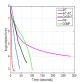
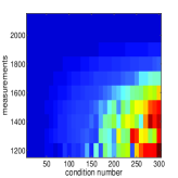
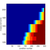
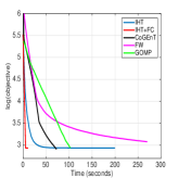
Figure 1: (From left to right) Objective value as a function of time for various methods, when data is well conditioned and poorly conditioned. The latter two figures show the phase transition plots for poorly conditioned data, for IHT and GOMP respectively.

In this section, we empirically compare and contrast our proposed group IHT methods against the existing approaches to solve the overlapping group sparsity problem. At a high level, we observe that our proposed variants of IHT indeed outperforms the existing state-of-the-art methods for group-sparse regression in terms of time complexity. Encouragingly, IHT also performs competitively with the existing methods in terms of accuracy. In fact, our results on the breast cancer dataset shows a 10%percent1010\% relative improvement in accuracy over existing methods.

Greedy methods for group sparsity have been shown to outperform proximal point schemes, and hence we restrict our comparison to greedy procedures. We compared four methods: our algorithm with (IHT-FC) and without (IHT) the fully corrective step, the Frank Wolfe (FW) method [21] , CoGEnT, [17] and the Group OMP (GOMP) [20]. All relevant hyper-parameters were chosen via a grid search, and experiments were run on a macbook laptop with a 2.5 GHz processor and 16gb memory. Additional experimental results are presented in Appendix G
Refer to caption
Refer to caption
Method Error %percent\% time (sec)
FW 29.41 6.4538
IHT 27.94 0.04000.0400\bm{0.0400}
GOMP 25.0125.01{25.01} 0.2891
CoGEnT 23.53 0.1414
IHT-FC 21.6521.65\bm{21.65} 0.1601
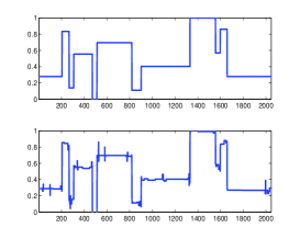
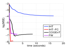
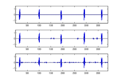
Figure 2: (Left) SoG: error vs time comparison for various methods, (Center) SoG: reconstruction of the true signal (top) from IHT-FC (middle) and CoGEnT (bottom). (Right:) Tumor Classification: misclassification rate of various methods.

Synthetic Data, well conditioned: We first compared various greedy schemes for solving the overlapping group sparsity problem on synthetic data. We generated M=1000𝑀1000M=1000 groups of contiguous indices of size 25; the last 555 entries of one group overlap with the first 555 of the next. We randomly set 505050 of these to be active, populated by uniform [1,1]11[-1,1] entries. This yields 𝒘p,p22000formulae-sequencesuperscript𝒘superscript𝑝similar-to𝑝22000\bm{w}^{\star}\in\mathbb{R}^{p},\leavevmode\nobreak\ \ p\sim 22000. 𝑿n×p𝑿superscript𝑛𝑝\bm{X}\in\mathbb{R}^{n\times p} where n=5000𝑛5000n=5000 and Xiji.i.dN(0,1)superscriptsimilar-toformulae-sequence𝑖𝑖𝑑subscript𝑋𝑖𝑗𝑁01X_{ij}\stackrel{{\scriptstyle i.i.d}}{{\sim}}N(0,1). Each measurement is corrupted with Additive White Gaussian Noise (AWGN) with standard deviation λ=0.1𝜆0.1\lambda=0.1. IHT mehods achieve orders of magnitude speedup compared to the competing schemes, and achieve almost the same (final) objective function value despite approximate projections (Figure 1 (Left)).

Synthetic Data, poorly conditioned: Next, we consider the exact same setup, but with each row of X𝑋X given by: 𝒙iN(0,Σ)similar-tosubscript𝒙𝑖𝑁0Σ\bm{x}_{i}\sim N(0,\Sigma) where κ=σmax(Σ)/σmin(Σ)=10𝜅subscript𝜎Σsubscript𝜎Σ10\kappa=\sigma_{\max}(\Sigma)/\sigma_{\min}(\Sigma)=10. Figure 1 (Center-left) shows again the advantages of using IHT methods; IHT-FC is about 10 times faster than the next best CoGEnT.

We next generate phase transition plots for recovery by our method (IHT) as well as the state-of-the-art GOMP method. We generate vectors in the same vein as the above experiment, with M=500,B=15,k=25,p5000formulae-sequence𝑀500formulae-sequence𝐵15formulae-sequence𝑘25similar-to𝑝5000M=500,\leavevmode\nobreak\ \ B=15,\leavevmode\nobreak\ \ k=25,\leavevmode\nobreak\ \ p\sim 5000. We vary the the condition number of the data covariance (ΣΣ\Sigma) as well as the number of measurements (n𝑛n). Figure 1 (Center-right and Right) shows the phase transition plot as the measurements and the condition number are varied for IHT, and GOMP respectively. The results are averaged over 10 independent runs. It can be seen that even for condition numbers as high as 200, n1500similar-to𝑛1500n\sim 1500 measurements suffices for IHT to exactly recovery 𝒘superscript𝒘\bm{w}^{*}, whereas GOMP with the same setting is not able to recover 𝒘superscript𝒘\bm{w}^{*} even once.

Tumor Classification, Breast Cancer Dataset

We next compare the aforementioned methods on a gene selection problem for breast cancer tumor classification. We use the data used in [9] 222download at http://cbio.ensmp.fr/ljacob/http://cbio.ensmp.fr/\leavevmode\nobreak\ ljacob/. We ran a 5-fold cross validation scheme to choose parameters, where we varied η{25,24,,23}k{2,5,10,15,20,50,100}τ{23,24,,213}formulae-sequence𝜂superscript25superscript24superscript23formulae-sequence𝑘2510152050100𝜏superscript23superscript24superscript213\eta\in\{2^{-5},2^{-4},\ldots,2^{3}\}\leavevmode\nobreak\ \ k\in\{2,5,10,15,20,50,100\}\leavevmode\nobreak\ \ \tau\in\{2^{3},2^{4},\ldots,2^{13}\}. Figure 2 (Right) shows that the vanilla hard thresholding method is competitive despite performing approximate projections, and the method with full corrections obtains the best performance among the methods considered. We randomly chose 15%percent1515\% of the data to test on.
Sparse Overlapping Group Lasso: Finally, we study the sparse overlapping group (SoG) problem that was introduced and analyzed in [16] (Figure 2). We perform projections as detailed in Algorithm 3. We generated synthetic vectors with 100 groups of size 50 and randomly selected 555 groups to be active, and among the active group only set 303030 coefficients to be non zero. The groups themselves were overlapping, with the last 10 entries of one group shared with the first 10 of the next, yielding p4000similar-to𝑝4000p\sim 4000. We chose the best parameters from a grid, and we set k=2k𝑘2superscript𝑘k=2k^{*} for the IHT methods.

6 Conclusions and Discussion

We proposed a greedy-IHT method that can applied to regression problems over set of group sparse vectors. Our proposed solution is efficient, scalable, and provide fast convergence guarantees under general RSC/RSS style conditions, unlike existing methods. We extended our analysis to handle even more challenging structures like sparse overlapping groups. Our experiments show that IHT methods achieve fast, accurate results even with greedy and approximate projections.

References

  • [1] Francis Bach. Convex analysis and optimization with submodular functions: A tutorial. arXiv preprint arXiv:1010.4207, 2010.
  • [2] Richard G Baraniuk, Volkan Cevher, Marco F Duarte, and Chinmay Hegde. Model-based compressive sensing. Information Theory, IEEE Transactions on, 56(4):1982–2001, 2010.
  • [3] Nirav Bhan, Luca Baldassarre, and Volkan Cevher. Tractability of interpretability via selection of group-sparse models. In Information Theory Proceedings (ISIT), 2013 IEEE International Symposium on, pages 1037–1041. IEEE, 2013.
  • [4] Thomas Blumensath. Sampling and reconstructing signals from a union of linear subspaces. Information Theory, IEEE Transactions on, 57(7):4660–4671, 2011.
  • [5] Thomas Blumensath and Mike E Davies. Sampling theorems for signals from the union of finite-dimensional linear subspaces. Information Theory, IEEE Transactions on, 55(4):1872–1882, 2009.
  • [6] Thomas Blumensath and Mike E Davies. Normalized iterative hard thresholding: Guaranteed stability and performance. Selected Topics in Signal Processing, IEEE Journal of, 4(2):298–309, 2010.
  • [7] Chinmay Hegde, Piotr Indyk, and Ludwig Schmidt. Approximation algorithms for model-based compressive sensing. Information Theory, IEEE Transactions on, 61(9):5129–5147, 2015.
  • [8] Junzhou Huang, Tong Zhang, and Dimitris Metaxas. Learning with structured sparsity. The Journal of Machine Learning Research, 12:3371–3412, 2011.
  • [9] Laurent Jacob, Guillaume Obozinski, and Jean-Philippe Vert. Group lasso with overlap and graph lasso. In Proceedings of the 26th annual International Conference on Machine Learning, pages 433–440. ACM, 2009.
  • [10] Prateek Jain, Ambuj Tewari, and Inderjit S Dhillon. Orthogonal matching pursuit with replacement. In Advances in Neural Information Processing Systems, pages 1215–1223, 2011.
  • [11] Prateek Jain, Ambuj Tewari, and Purushottam Kar. On iterative hard thresholding methods for high-dimensional m-estimation. In Advances in Neural Information Processing Systems, pages 685–693, 2014.
  • [12] Rodolphe Jenatton, Julien Mairal, Francis R Bach, and Guillaume R Obozinski. Proximal methods for sparse hierarchical dictionary learning. In Proceedings of the 27th International Conference on Machine Learning (ICML-10), pages 487–494, 2010.
  • [13] Anastasios Kyrillidis and Volkan Cevher. Combinatorial selection and least absolute shrinkage via the clash algorithm. In Information Theory Proceedings (ISIT), 2012 IEEE International Symposium on, pages 2216–2220. IEEE, 2012.
  • [14] Karim Lounici, Massimiliano Pontil, Alexandre B Tsybakov, and Sara Van De Geer. Taking advantage of sparsity in multi-task learning. arXiv preprint arXiv:0903.1468, 2009.
  • [15] George L Nemhauser, Laurence A Wolsey, and Marshall L Fisher. An analysis of approximations for maximizing submodular set functions. Mathematical Programming, 14(1):265–294, 1978.
  • [16] Nikhil Rao, Christopher Cox, Rob Nowak, and Timothy T Rogers. Sparse overlapping sets lasso for multitask learning and its application to fmri analysis. In Advances in neural information processing systems, pages 2202–2210, 2013.
  • [17] Nikhil Rao, Parikshit Shah, and Stephen Wright. Forward–backward greedy algorithms for atomic norm regularization. Signal Processing, IEEE Transactions on, 63(21):5798–5811, 2015.
  • [18] Nikhil S Rao, Ben Recht, and Robert D Nowak. Universal measurement bounds for structured sparse signal recovery. In International Conference on Artificial Intelligence and Statistics, pages 942–950, 2012.
  • [19] Parikshit Shah and Venkat Chandrasekaran. Iterative projections for signal identification on manifolds: Global recovery guarantees. In Communication, Control, and Computing (Allerton), 2011 49th Annual Allerton Conference on, pages 760–767. IEEE, 2011.
  • [20] Grzegorz Swirszcz, Naoki Abe, and Aurelie C Lozano. Grouped orthogonal matching pursuit for variable selection and prediction. In Advances in Neural Information Processing Systems, pages 1150–1158, 2009.
  • [21] Ambuj Tewari, Pradeep K Ravikumar, and Inderjit S Dhillon. Greedy algorithms for structurally constrained high dimensional problems. In Advances in Neural Information Processing Systems, pages 882–890, 2011.
  • [22] Joel Tropp, Anna C Gilbert, et al. Signal recovery from random measurements via orthogonal matching pursuit. Information Theory, IEEE Transactions on, 53(12):4655–4666, 2007.
  • [23] Sara A Van De Geer, Peter Bühlmann, et al. On the conditions used to prove oracle results for the lasso. Electronic Journal of Statistics, 3:1360–1392, 2009.
  • [24] Xiaotong Yuan, Ping Li, and Tong Zhang. Gradient hard thresholding pursuit for sparsity-constrained optimization. In Proceedings of the 31st International Conference on Machine Learning (ICML-14), pages 127–135, 2014.

Appendix A Using submodularity to perform projections

While solving (6) is NP-hard in general, the authors in [3] showed that it can be approximately solved using methods from submodular function optimization, which we quickly recap here. First, (6) can be cast in the following equivalent way:

𝒢^=argmax|𝒢~|k{iI𝒈i2:I=G𝒢~G}\hat{\mathcal{G}}=\arg\max_{|\tilde{\mathcal{G}}|\leq k}\left\{\sum_{i\in I}\bm{g}_{i}^{2}:\leavevmode\nobreak\ \ I=\cup_{G\in{\tilde{\mathcal{G}}}}G\right\} (8)

Once we have 𝒢^^𝒢\hat{\mathcal{G}}, 𝒖^^𝒖\hat{\bm{u}} can be recovered by simply setting 𝒖^I=𝒈Isubscript^𝒖𝐼subscript𝒈𝐼\hat{\bm{u}}_{I}=\bm{g}_{I} and 00 everywhere else, where I=G𝒢^G𝐼subscript𝐺^𝒢𝐺I=\cup_{G\in\hat{\mathcal{G}}}G. Next, we have the following result

Lemma A.1.

Given a set S[p]𝑆delimited-[]𝑝S\in[p], the function z(S)=iS𝐱i2.𝑧𝑆subscript𝑖𝑆superscriptsubscript𝐱𝑖2z(S)=\sum_{i\in S}\bm{x}_{i}^{2}. is submodular.

Proof.

First, recall the definition of a submodular function:

Definition A.2.

Let Q𝑄Q be a finite set, and let z()𝑧z(\cdot) be a real valued function defined on ΩQsuperscriptΩ𝑄\Omega^{Q}, the power set of Q𝑄Q. The function z()𝑧z(\cdot) is said to be submodular if

z(S)+z(T)z(ST)+z(ST)S,TΩQformulae-sequence𝑧𝑆𝑧𝑇𝑧𝑆𝑇𝑧𝑆𝑇for-all𝑆𝑇superscriptΩ𝑄z(S)+z(T)\geq z(S\cup T)+z(S\cap T)\leavevmode\nobreak\ \ \forall S,T\subset\Omega^{Q}

Let S𝑆S and T𝑇T be two sets of groups, s.t., ST𝑆𝑇S\subseteq T. Let, SS=supp(jSGj)𝑆𝑆suppsubscript𝑗𝑆subscript𝐺𝑗SS=\operatorname{supp}(\cup_{j\in S}G_{j}) and TT=supp(jTGj)𝑇𝑇suppsubscript𝑗𝑇subscript𝐺𝑗TT=\operatorname{supp}(\cup_{j\in T}G_{j}). Then, SSTT𝑆𝑆𝑇𝑇SS\subseteq TT. Hence,

z(Si)z(S)𝑧𝑆𝑖𝑧𝑆\displaystyle z(S\cup i)-z(S) =SSsupp(Gi)𝒙2SS𝒙2absentsubscript𝑆𝑆suppsubscript𝐺𝑖superscriptsubscript𝒙2subscript𝑆𝑆superscriptsubscript𝒙2\displaystyle=\sum_{\ell\in SS\cup\operatorname{supp}(G_{i})}\bm{x}_{\ell}^{2}-\sum_{\ell\in SS}\bm{x}_{\ell}^{2}
=supp(Gi)\SS𝒙2ζ1supp(Gi)\TT𝒙=z(Ti)z(T),absentsubscript\suppsubscript𝐺𝑖𝑆𝑆superscriptsubscript𝒙2superscriptsubscript𝜁1subscript\suppsubscript𝐺𝑖𝑇𝑇subscript𝒙𝑧𝑇𝑖𝑧𝑇\displaystyle=\sum_{\ell\in\operatorname{supp}(G_{i})\backslash SS}\bm{x}_{\ell}^{2}\stackrel{{\scriptstyle\zeta_{1}}}{{\geq}}\sum_{\ell\in\operatorname{supp}(G_{i})\backslash TT}\bm{x}_{\ell}=z(T\cup i)-z(T),

where ζ1subscript𝜁1\zeta_{1} follows from SSTT𝑆𝑆𝑇𝑇SS\subseteq TT. This completes the proof. ∎

This result shows that (8) can be cast as a problem of the form

maxSQz(S),s.t.|S|k.subscript𝑆𝑄𝑧𝑆s.t.𝑆𝑘\max_{S\subset Q}z(S),\ \text{s.t.}\leavevmode\nobreak\ \ |S|\leq k. (9)

Algorithm 2, which details the pseudocode for performing approximate projections, exactly corresponds to the greedy algorithm for submodular optimization [1], and this gives us a means to assess the quality of our projections.

A.1 Proof of Lemma 2.2

Proof.

First, from the approximation property of the greedy algorithm [15],

𝒖^2(1ekk)𝒖2superscriptnorm^𝒖21superscript𝑒superscript𝑘𝑘superscriptnormsubscript𝒖2\|\hat{\bm{u}}\|^{2}\geq\left(1-e^{-\frac{k^{\prime}}{k}}\right)\|\bm{u}_{*}\|^{2} (10)

Also, 𝒈𝒖^2=𝒈2𝒖^2superscriptnorm𝒈^𝒖2superscriptnorm𝒈2superscriptnorm^𝒖2\|\bm{g}-\hat{\bm{u}}\|^{2}=\|\bm{g}\|^{2}-\|\hat{\bm{u}}\|^{2} because (𝒖^)supp(𝒖^)=(𝒈)supp(𝒖^)subscript^𝒖supp^𝒖subscript𝒈supp^𝒖(\hat{\bm{u}})_{\operatorname{supp}(\hat{\bm{u}})}=(\bm{g})_{\operatorname{supp}(\hat{\bm{u}})} and 00 otherwise.

Using the above two equations, we have:

𝒈𝒖^2superscriptnorm𝒈^𝒖2\displaystyle\|\bm{g}-\hat{\bm{u}}\|^{2} 𝒈2𝒖2+ekk𝒖2,absentsuperscriptnorm𝒈2superscriptnormsubscript𝒖2superscript𝑒superscript𝑘𝑘superscriptnormsubscript𝒖2\displaystyle\leq\|\bm{g}\|^{2}-\|\bm{u}_{*}\|^{2}+e^{-\frac{k^{\prime}}{k}}\|\bm{u}_{*}\|^{2},
=𝒈𝒖2+ekk𝒖2,absentsuperscriptnorm𝒈subscript𝒖2superscript𝑒superscript𝑘𝑘superscriptnormsubscript𝒖2\displaystyle=\|\bm{g}-\bm{u}_{*}\|^{2}+e^{-\frac{k^{\prime}}{k}}\|\bm{u}_{*}\|^{2},
=𝒈𝒖2+ekk(𝒈)supp(𝒖)2,absentsuperscriptnorm𝒈subscript𝒖2superscript𝑒superscript𝑘𝑘superscriptnormsubscript𝒈suppsubscript𝒖2\displaystyle=\|\bm{g}-\bm{u}_{*}\|^{2}+e^{-\frac{k^{\prime}}{k}}\|(\bm{g})_{\operatorname{supp}(\bm{u}_{*})}\|^{2}, (11)

where both equalities above follow from the fact that due to optimality, (𝒖)supp(𝒖)=(𝒈)supp(𝒖)subscriptsubscript𝒖suppsubscript𝒖subscript𝒈suppsubscript𝒖(\bm{u}_{*})_{\operatorname{supp}(\bm{u}_{*})}=(\bm{g})_{\operatorname{supp}(\bm{u}_{*})}.

Appendix B Proof of Theorem 3.1

Proof.

Recall that 𝒈t=𝒘tηf(𝒘t)subscript𝒈𝑡subscript𝒘𝑡𝜂𝑓subscript𝒘𝑡\bm{g}_{t}=\bm{w}_{t}-\eta\nabla f(\bm{w}_{t}), 𝒘t+1=P^k𝒢(𝒈t)subscript𝒘𝑡1superscriptsubscript^𝑃𝑘𝒢subscript𝒈𝑡\bm{w}_{t+1}=\widehat{P}_{k}^{\mathcal{G}}(\bm{g}_{t}).

Let supp(𝒘t+1)=St+1suppsubscript𝒘𝑡1subscript𝑆𝑡1\operatorname{supp}(\bm{w}_{t+1})=S_{t+1}, supp(𝒘)=Ssuppsuperscript𝒘subscript𝑆\operatorname{supp}(\bm{w}^{*})=S_{*}, I=St+1S𝐼subscript𝑆𝑡1subscript𝑆I=S_{t+1}\cup S_{*}, and M=S\St+1𝑀\subscript𝑆subscript𝑆𝑡1M=S_{*}\backslash S_{t+1}. Also, note that |Gsupp(I)|k+kGsupp𝐼𝑘superscript𝑘|\operatorname{G-supp}(I)|\leq k+k^{*}.

Moreover, (𝒘t+1)St+1=(𝒈t)St+1subscriptsubscript𝒘𝑡1subscript𝑆𝑡1subscriptsubscript𝒈𝑡subscript𝑆𝑡1(\bm{w}_{t+1})_{S_{t+1}}=(\bm{g}_{t})_{S_{t+1}} (See Algorithm 2). Hence, (𝒘t+1𝒈t)St+1S22=(𝒈t)M22superscriptsubscriptnormsubscriptsubscript𝒘𝑡1subscript𝒈𝑡subscript𝑆𝑡1subscript𝑆22superscriptsubscriptnormsubscriptsubscript𝒈𝑡𝑀22\|(\bm{w}_{t+1}-\bm{g}_{t})_{S_{t+1}\cup S_{*}}\|_{2}^{2}=\|(\bm{g}_{t})_{M}\|_{2}^{2}.

Now, using Lemma B.2 with 𝒛=(𝒈t)I𝒛subscriptsubscript𝒈𝑡𝐼\bm{z}=(\bm{g}_{t})_{I},we have:

(𝒘t+1𝒈t)I22=(𝒈t)M22superscriptsubscriptnormsubscriptsubscript𝒘𝑡1subscript𝒈𝑡𝐼22superscriptsubscriptnormsubscriptsubscript𝒈𝑡𝑀22\displaystyle\|(\bm{w}_{t+1}-\bm{g}_{t})_{I}\|_{2}^{2}=\|(\bm{g}_{t})_{M}\|_{2}^{2} ζ1kkk~(𝒈t)St+1\S22+kϵkk~,superscriptsubscript𝜁1absentsuperscript𝑘𝑘~𝑘superscriptsubscriptnormsubscriptsubscript𝒈𝑡\subscript𝑆𝑡1subscript𝑆22superscript𝑘italic-ϵ𝑘~𝑘\displaystyle\stackrel{{\scriptstyle\zeta_{1}}}{{\leq}}\frac{k^{*}}{k-\widetilde{k}}\cdot\|(\bm{g}_{t})_{S_{t+1}\backslash S_{*}}\|_{2}^{2}+\frac{k^{*}\epsilon}{k-\widetilde{k}},
ζ2kkk~(𝒘𝒈t)I22+kϵkk~,superscriptsubscript𝜁2absentsuperscript𝑘𝑘~𝑘superscriptsubscriptnormsubscriptsuperscript𝒘subscript𝒈𝑡𝐼22superscript𝑘italic-ϵ𝑘~𝑘\displaystyle\stackrel{{\scriptstyle\zeta_{2}}}{{\leq}}\frac{k^{*}}{k-\widetilde{k}}\cdot\|(\bm{w}^{*}-\bm{g}_{t})_{I}\|_{2}^{2}+\frac{k^{*}\epsilon}{k-\widetilde{k}}, (12)

where ζ1subscript𝜁1\zeta_{1} follows from MS𝑀subscript𝑆M\subset S_{*} and hence |Gsupp(M)||Gsupp(S)|=kGsupp𝑀Gsuppsubscript𝑆superscript𝑘|\operatorname{G-supp}(M)|\leq|\operatorname{G-supp}(S_{*})|=k^{*}. ζ2subscript𝜁2\zeta_{2} follows since 𝒘St+1\S=0subscriptsuperscript𝒘\subscript𝑆𝑡1subscript𝑆0\bm{w}^{*}_{S_{t+1}\backslash S_{*}}=0.

Now, using the fact that (𝒘t+1𝒘)I2=𝒘t+1𝒘2subscriptnormsubscriptsubscript𝒘𝑡1superscript𝒘𝐼2subscriptnormsubscript𝒘𝑡1superscript𝒘2\|(\bm{w}_{t+1}-\bm{w}^{*})_{I}\|_{2}=\|\bm{w}_{t+1}-\bm{w}^{*}\|_{2} along with triangle inequality, we have:

𝒘t+1𝒘2subscriptnormsubscript𝒘𝑡1superscript𝒘2\displaystyle\|\bm{w}_{t+1}-\bm{w}^{*}\|_{2}
(1+kkk~)(𝒘𝒈t)I2+kϵkk~,absent1superscript𝑘𝑘~𝑘subscriptnormsubscriptsuperscript𝒘subscript𝒈𝑡𝐼2superscript𝑘italic-ϵ𝑘~𝑘\displaystyle\leq\left(1+\sqrt{\frac{k^{*}}{k-\widetilde{k}}}\right)\cdot\|(\bm{w}^{*}-\bm{g}_{t})_{I}\|_{2}+\sqrt{\frac{k^{*}\epsilon}{k-\widetilde{k}}}, (13)
ζ1(1+kkk~)(𝒘𝒘tη(f(𝒘)f(𝒘t)))I2+2η(f(𝒘))St+12+kϵkk~,superscriptsubscript𝜁1absent1superscript𝑘𝑘~𝑘subscriptnormsubscriptsuperscript𝒘subscript𝒘𝑡𝜂𝑓superscript𝒘𝑓subscript𝒘𝑡𝐼22𝜂subscriptnormsubscript𝑓superscript𝒘subscript𝑆𝑡12superscript𝑘italic-ϵ𝑘~𝑘\displaystyle\stackrel{{\scriptstyle\zeta_{1}}}{{\leq}}\left(1+\sqrt{\frac{k^{*}}{k-\widetilde{k}}}\right)\cdot\|(\bm{w}^{*}-\bm{w}_{t}-\eta(\nabla f(\bm{w}^{*})-\nabla f(\bm{w}_{t})))_{I}\|_{2}+2\eta\|(\nabla f(\bm{w}^{*}))_{S_{t+1}}\|_{2}+\sqrt{\frac{k^{*}\epsilon}{k-\widetilde{k}}},
ζ2(1+kkk~)(IηH(ISt)(ISt)(α))(𝒘t𝒘)ISt2+2η(f(𝒘))St+12+kϵkk~,superscriptsubscript𝜁2absent1superscript𝑘𝑘~𝑘subscriptnorm𝐼𝜂subscript𝐻𝐼subscript𝑆𝑡𝐼subscript𝑆𝑡𝛼subscriptsubscript𝒘𝑡superscript𝒘𝐼subscript𝑆𝑡22𝜂subscriptnormsubscript𝑓superscript𝒘subscript𝑆𝑡12superscript𝑘italic-ϵ𝑘~𝑘\displaystyle\stackrel{{\scriptstyle\zeta_{2}}}{{\leq}}\left(1+\sqrt{\frac{k^{*}}{k-\widetilde{k}}}\right)\cdot\|(I-\eta H_{(I\cup S_{t})(I\cup S_{t})}(\alpha))(\bm{w}_{t}-\bm{w}^{*})_{I\cup S_{t}}\|_{2}+2\eta\|(\nabla f(\bm{w}^{*}))_{S_{t+1}}\|_{2}+\sqrt{\frac{k^{*}\epsilon}{k-\widetilde{k}}},
ζ3(1+kkk~)(1α2k+kL2k+k)𝒘t𝒘2+2L2k+k(f(𝒘))St+12+kϵkk~,superscriptsubscript𝜁3absent1superscript𝑘𝑘~𝑘1subscript𝛼2𝑘superscript𝑘subscript𝐿2𝑘superscript𝑘subscriptnormsubscript𝒘𝑡superscript𝒘22subscript𝐿2𝑘superscript𝑘subscriptnormsubscript𝑓superscript𝒘subscript𝑆𝑡12superscript𝑘italic-ϵ𝑘~𝑘\displaystyle\stackrel{{\scriptstyle\zeta_{3}}}{{\leq}}\left(1+\sqrt{\frac{k^{*}}{k-\widetilde{k}}}\right)\cdot\left(1-\frac{\alpha_{2k+k^{*}}}{L_{2k+k^{*}}}\right)\|\bm{w}_{t}-\bm{w}^{*}\|_{2}+\frac{2}{L_{2k+k^{*}}}\|(\nabla f(\bm{w}^{*}))_{S_{t+1}}\|_{2}+\sqrt{\frac{k^{*}\epsilon}{k-\widetilde{k}}},

where α=c𝒘t+(1c)𝒘𝛼𝑐subscript𝒘𝑡1𝑐superscript𝒘\alpha=c\bm{w}_{t}+(1-c)\bm{w}^{*} for c>0𝑐0c>0 and H(α)𝐻𝛼H(\alpha) is the Hessian of f𝑓f evaluated at α𝛼\alpha. ζ1subscript𝜁1\zeta_{1} follows from triangle inequality, ζ2subscript𝜁2\zeta_{2} follows from the Mean-Value theorem and ζ3subscript𝜁3\zeta_{3} follows from the RSC/RSS condition and by setting η=1/L2k+k𝜂1subscript𝐿2𝑘superscript𝑘\eta=1/L_{2k+k^{*}}.

The theorem now follows by setting k=2((L2k+kα2k+k)2+1)log(𝒘2/ϵ)𝑘2superscriptsubscript𝐿2𝑘superscript𝑘subscript𝛼2𝑘superscript𝑘21subscriptnormsuperscript𝒘2italic-ϵk=2\left(\left(\frac{L_{2k+k^{*}}}{\alpha_{2k+k^{*}}}\right)^{2}+1\right)\cdot\log(\|\bm{w}^{*}\|_{2}/\epsilon) and ϵitalic-ϵ\epsilon appropriately.

Lemma B.1.

Let 𝐰=P^k𝒢(𝐠)𝐰superscriptsubscript^𝑃𝑘𝒢𝐠\bm{w}=\widehat{P}_{k}^{\mathcal{G}}(\bm{g}) and let S=supp(𝐰)𝑆supp𝐰S=\operatorname{supp}(\bm{w}). Then, for every I𝐼I s.t. SI𝑆𝐼S\subseteq I, the following holds:

𝒘I=P^k𝒢(gI).subscript𝒘𝐼superscriptsubscript^𝑃𝑘𝒢subscript𝑔𝐼\bm{w}_{I}=\widehat{P}_{k}^{\mathcal{G}}(g_{I}).
Proof.

Let Q={i1,i2,,ik}𝑄subscript𝑖1subscript𝑖2subscript𝑖𝑘Q=\{i_{1},i_{2},\dots,i_{k}\} be the k𝑘k-groups selected when the greedy procedure (Algorithm 2) is applied to 𝒈𝒈\bm{g}. Then,

𝒘Gij\(1j1Gi)22𝒘Gi\(1j1Gi)22,1jk,iQ.formulae-sequenceformulae-sequencesuperscriptsubscriptnormsubscript𝒘\subscript𝐺subscript𝑖𝑗subscript1𝑗1subscript𝐺subscript𝑖22superscriptsubscriptnormsubscript𝒘\subscript𝐺𝑖subscript1𝑗1subscript𝐺subscript𝑖22for-all1𝑗𝑘for-all𝑖𝑄\|\bm{w}_{G_{i_{j}}\backslash(\cup_{1\leq\ell\leq j-1}G_{i_{\ell}})}\|_{2}^{2}\geq\|\bm{w}_{G_{i}\backslash(\cup_{1\leq\ell\leq j-1}G_{i_{\ell}})}\|_{2}^{2},\ \forall 1\leq j\leq k,\ \forall i\notin Q.

Moreover, the greedy selection procedure is deterministic. Hence, even if groups Gisubscript𝐺𝑖G_{i} are restricted to lie in a subset of 𝒢𝒢\mathcal{G}, the output of the procedure remains exactly the same. ∎

Lemma B.2.

Let 𝐳p𝐳superscript𝑝\bm{z}\in\mathbb{R}^{p} be any vector. Let 𝐰^=P^k𝒢(𝐳)^𝐰superscriptsubscript^𝑃𝑘𝒢𝐳\widehat{\bm{w}}=\widehat{P}_{k}^{\mathcal{G}}(\bm{z}) and let 𝐰psuperscript𝐰superscript𝑝\bm{w}^{*}\in\mathbb{R}^{p} be s.t. |Gsupp(𝐰)|kGsuppsuperscript𝐰superscript𝑘|\operatorname{G-supp}(\bm{w}^{*})|\leq k^{*}. Let S=supp(𝐰^)𝑆supp^𝐰S=\operatorname{supp}(\widehat{\bm{w}}), S=supp(𝐰)subscript𝑆suppsuperscript𝐰S_{*}=\operatorname{supp}(\bm{w}^{*}), I=SS𝐼𝑆subscript𝑆I=S\cup S_{*}, and M=S\S𝑀\subscript𝑆𝑆M=S_{*}\backslash S. Then, the following holds:

𝒛M22kϵkk~𝒛S\S22kk~,superscriptsubscriptnormsubscript𝒛𝑀22superscript𝑘italic-ϵ𝑘~𝑘superscriptsubscriptnormsubscript𝒛\𝑆superscript𝑆22𝑘~𝑘\frac{\|\bm{z}_{M}\|_{2}^{2}}{k^{*}}-\frac{\epsilon}{k-\widetilde{k}}\leq\frac{\|\bm{z}_{S\backslash S^{*}}\|_{2}^{2}}{k-\widetilde{k}},

where k~=O(klog(𝐰2/ϵ))~𝑘𝑂superscript𝑘subscriptnormsuperscript𝐰2italic-ϵ\widetilde{k}=O(k^{*}\log(\|\bm{w}^{*}\|_{2}/\epsilon)).

Proof.

Recall that the k𝑘k groups are added greedily to form S=supp(𝒘^)𝑆supp^𝒘S=\operatorname{supp}(\widehat{\bm{w}}). Let Q={i1,i2,,ik}𝑄subscript𝑖1subscript𝑖2subscript𝑖𝑘Q=\{i_{1},i_{2},\dots,i_{k}\} be the k𝑘k-groups selected when the greedy procedure (Algorithm 2) is applied to 𝒛𝒛\bm{z}. Then,

𝒛Gij\(1j1Gi)22𝒛Gi\(1j1Gi)22,1jk,iQ.formulae-sequenceformulae-sequencesuperscriptsubscriptnormsubscript𝒛\subscript𝐺subscript𝑖𝑗subscript1𝑗1subscript𝐺subscript𝑖22superscriptsubscriptnormsubscript𝒛\subscript𝐺𝑖subscript1𝑗1subscript𝐺subscript𝑖22for-all1𝑗𝑘for-all𝑖𝑄\|\bm{z}_{G_{i_{j}}\backslash(\cup_{1\leq\ell\leq j-1}G_{i_{\ell}})}\|_{2}^{2}\geq\|\bm{z}_{G_{i}\backslash(\cup_{1\leq\ell\leq j-1}G_{i_{\ell}})}\|_{2}^{2},\ \ \ \forall 1\leq j\leq k,\ \ \forall i\notin Q.

Now, as 1j1GiS,1jkformulae-sequencesubscript1𝑗1subscript𝐺subscript𝑖𝑆for-all1𝑗𝑘\cup_{1\leq\ell\leq j-1}G_{i_{\ell}}\subseteq S,\ \forall 1\leq j\leq k, we have:

𝒛Gij\(1j1Gi)22𝒛Gi\S22,1jk,iQ.formulae-sequenceformulae-sequencesuperscriptsubscriptnormsubscript𝒛\subscript𝐺subscript𝑖𝑗subscript1𝑗1subscript𝐺subscript𝑖22superscriptsubscriptnormsubscript𝒛\subscript𝐺𝑖𝑆22for-all1𝑗𝑘for-all𝑖𝑄\|\bm{z}_{G_{i_{j}}\backslash(\cup_{1\leq\ell\leq j-1}G_{i_{\ell}})}\|_{2}^{2}\geq\|\bm{z}_{G_{i}\backslash S}\|_{2}^{2},\ \ \ \forall 1\leq j\leq k,\ \ \forall i\notin Q.

Let Gsupp(𝒘)={1,,k}Gsuppsuperscript𝒘subscript1subscriptsuperscript𝑘\operatorname{G-supp}(\bm{w}^{*})=\{\ell_{1},\dots,\ell_{k^{*}}\}. Then, adding the above inequalities for each jsubscript𝑗\ell_{j} s.t. jQsubscript𝑗𝑄\ell_{j}\notin Q, we get:

𝒛Gij\(1j1Gi)22𝒛S\S22k,superscriptsubscriptnormsubscript𝒛\subscript𝐺subscript𝑖𝑗subscript1𝑗1subscript𝐺subscript𝑖22superscriptsubscriptnormsubscript𝒛\superscript𝑆𝑆22superscript𝑘\|\bm{z}_{G_{i_{j}}\backslash(\cup_{1\leq\ell\leq j-1}G_{i_{\ell}})}\|_{2}^{2}\geq\frac{\|\bm{z}_{S^{*}\backslash S}\|_{2}^{2}}{k^{*}}, (15)

where the above inequality also uses the fact that jGsupp(𝒘),jQ𝒛Gj\S22𝒛S\S22subscriptformulae-sequencesubscript𝑗Gsuppsuperscript𝒘subscript𝑗𝑄superscriptsubscriptnormsubscript𝒛\subscript𝐺subscript𝑗𝑆22superscriptsubscriptnormsubscript𝒛\superscript𝑆𝑆22\sum_{\ell_{j}\in\operatorname{G-supp}(\bm{w}^{*}),\ell_{j}\notin Q}\|\bm{z}_{G_{\ell_{j}}\backslash S}\|_{2}^{2}\geq\|\bm{z}_{S^{*}\backslash S}\|_{2}^{2}.

Adding (15) (k~+1)jkfor-all~𝑘1𝑗𝑘\forall\ (\widetilde{k}+1)\leq j\leq k, we get:

𝒛S22𝒛B22kk~k𝒛S\S22,superscriptsubscriptnormsubscript𝒛𝑆22superscriptsubscriptnormsubscript𝒛𝐵22𝑘~𝑘superscript𝑘superscriptsubscriptnormsubscript𝒛\superscript𝑆𝑆22\|\bm{z}_{S}\|_{2}^{2}-\|\bm{z}_{B}\|_{2}^{2}\geq\frac{k-\widetilde{k}}{k^{*}}\cdot\|\bm{z}_{S^{*}\backslash S}\|_{2}^{2}, (16)

where B=1jk~Gij𝐵subscript1𝑗~𝑘subscript𝐺subscript𝑖𝑗B={\cup_{1\leq j\leq\widetilde{k}}G_{i_{j}}}.

Moreover using Lemma 2.2 and the fact that |Gsupp(𝒛S)|kGsuppsubscript𝒛superscript𝑆superscript𝑘|\operatorname{G-supp}(\bm{z}_{S^{*}})|\leq k^{*}, we get: 𝒛B22𝒛S22ϵsuperscriptsubscriptnormsubscript𝒛𝐵22superscriptsubscriptnormsubscript𝒛superscript𝑆22italic-ϵ\|\bm{z}_{B}\|_{2}^{2}\geq\|\bm{z}_{S^{*}}\|_{2}^{2}-\epsilon. Hence,

𝒛M22ksuperscriptsubscriptnormsubscript𝒛𝑀22superscript𝑘\displaystyle\frac{\|\bm{z}_{M}\|_{2}^{2}}{k^{*}} 𝒛S22𝒛B22kk~𝒛S22𝒛S22+ϵkk~𝒛S\S22+ϵkk~.absentsuperscriptsubscriptnormsubscript𝒛𝑆22superscriptsubscriptnormsubscript𝒛𝐵22𝑘~𝑘superscriptsubscriptnormsubscript𝒛𝑆22superscriptsubscriptnormsubscript𝒛superscript𝑆22italic-ϵ𝑘~𝑘superscriptsubscriptnormsubscript𝒛\𝑆superscript𝑆22italic-ϵ𝑘~𝑘\displaystyle\leq\frac{\|\bm{z}_{S}\|_{2}^{2}-\|\bm{z}_{B}\|_{2}^{2}}{k-\widetilde{k}}\leq\frac{\|\bm{z}_{S}\|_{2}^{2}-\|\bm{z}_{S^{*}}\|_{2}^{2}+\epsilon}{k-\widetilde{k}}\leq\frac{\|\bm{z}_{S\backslash S^{*}}\|_{2}^{2}+\epsilon}{k-\widetilde{k}}. (17)

Lemma now follows by a simple manipulation of the above given inequality. ∎

Appendix C Proof of Lemma 3.3

Proof.

Note that,

X𝒘22=i(𝒙iT𝒘)2=i(𝒛iTΣ1/2𝒘)2=ZΣ1/2𝒘22,superscriptsubscriptnorm𝑋𝒘22subscript𝑖superscriptsuperscriptsubscript𝒙𝑖𝑇𝒘2subscript𝑖superscriptsuperscriptsubscript𝒛𝑖𝑇superscriptΣ12𝒘2superscriptsubscriptnorm𝑍superscriptΣ12𝒘22\|X\bm{w}\|_{2}^{2}=\sum_{i}(\bm{x}_{i}^{T}\bm{w})^{2}=\sum_{i}(\bm{z}_{i}^{T}\Sigma^{1/2}\bm{w})^{2}=\|Z\Sigma^{1/2}\bm{w}\|_{2}^{2},

where Zn×p𝑍superscript𝑛𝑝Z\in\mathbb{R}^{n\times p} s.t. each row 𝒛iN(0,I)similar-tosubscript𝒛𝑖𝑁0𝐼\bm{z}_{i}\sim N(0,I) is a standard multivariate Gaussian. Now, using Theorem 1 of [5], and using the fact that Σ1/2𝒘superscriptΣ12𝒘\Sigma^{1/2}\bm{w} lies in a union of (Mk)binomial𝑀𝑘{M\choose k} subspaces each of at most s𝑠s dimensions, we have (w.p.11/(Mk2s))\left(w.p.\geq 1-1/(M^{k}\cdot 2^{s})\right):

(14C)Σ1/2𝒘221nZΣ1/2𝒘22(1+4C)Σ1/2𝒘22.14𝐶superscriptsubscriptnormsuperscriptΣ12𝒘221𝑛superscriptsubscriptnorm𝑍superscriptΣ12𝒘2214𝐶superscriptsubscriptnormsuperscriptΣ12𝒘22\left(1-\frac{4}{\sqrt{C}}\right)\|\Sigma^{1/2}\bm{w}\|_{2}^{2}\leq\frac{1}{n}\|Z\Sigma^{1/2}\bm{w}\|_{2}^{2}\leq\left(1+\frac{4}{\sqrt{C}}\right)\|\Sigma^{1/2}\bm{w}\|_{2}^{2}.

The result follows by using the definition of σminsubscript𝜎\sigma_{\min} and σmaxsubscript𝜎\sigma_{\max}. ∎

Appendix D Proof of Theorem 3.4

Proof.

Recall that 𝒈t=𝒘tηf(𝒘t)subscript𝒈𝑡subscript𝒘𝑡𝜂𝑓subscript𝒘𝑡\bm{g}_{t}=\bm{w}_{t}-\eta\nabla f(\bm{w}_{t}), 𝒘t+1=Pk𝒢(𝒈t)subscript𝒘𝑡1superscriptsubscript𝑃𝑘𝒢subscript𝒈𝑡\bm{w}_{t+1}=P_{k}^{\mathcal{G}}(\bm{g}_{t}). Similar to the proof of Theorem 3.1 (Appendix B), we define St+1=supp(𝒘t+1)subscript𝑆𝑡1suppsubscript𝒘𝑡1S_{t+1}=\operatorname{supp}(\bm{w}_{t+1}), St=supp(𝒘t)subscript𝑆𝑡suppsubscript𝒘𝑡S_{t}=\operatorname{supp}(\bm{w}_{t}), S=supp(𝒘)subscript𝑆suppsuperscript𝒘S_{*}=\operatorname{supp}(\bm{w}^{*}), I=St+1S𝐼subscript𝑆𝑡1subscript𝑆I=S_{t+1}\cup S_{*}, J=ISt𝐽𝐼subscript𝑆𝑡J=I\cup S_{t}, and M=S\St+1𝑀\subscript𝑆subscript𝑆𝑡1M=S_{*}\backslash S_{t+1}. Also, note that |Gsupp(I)|k+kGsupp𝐼𝑘superscript𝑘|\operatorname{G-supp}(I)|\leq k+k^{*}, |Gsupp(J)|2k+kGsupp𝐽2𝑘superscript𝑘|\operatorname{G-supp}(J)|\leq 2k+k^{*}.

Now, using Lemma D.1 with 𝒛=(𝒈t)I𝒛subscriptsubscript𝒈𝑡𝐼\bm{z}=(\bm{g}_{t})_{I}, we have: (𝒘t+1𝒈t)I22kk(𝒘𝒈t)I22superscriptsubscriptnormsubscriptsubscript𝒘𝑡1subscript𝒈𝑡𝐼22superscript𝑘𝑘superscriptsubscriptnormsubscriptsuperscript𝒘subscript𝒈𝑡𝐼22\|(\bm{w}_{t+1}-\bm{g}_{t})_{I}\|_{2}^{2}\leq\frac{k^{*}}{k}\cdot\|(\bm{w}^{*}-\bm{g}_{t})_{I}\|_{2}^{2}. This follows from noting that M=k+kM=k+k* here. Now, the remaining proof follows proof of Theorem 3.1 closely. That is, using the above inequality with triangle inequality, we have:

𝒘t+1𝒘2subscriptnormsubscript𝒘𝑡1superscript𝒘2\displaystyle\|\bm{w}_{t+1}-\bm{w}^{*}\|_{2}
(1+kk)(𝒘𝒈t)I2absent1superscript𝑘𝑘subscriptnormsubscriptsuperscript𝒘subscript𝒈𝑡𝐼2\displaystyle\leq\left(1+\sqrt{\frac{k^{*}}{k}}\right)\cdot\|(\bm{w}^{*}-\bm{g}_{t})_{I}\|_{2}
ζ1(1+kk)(𝒘𝒘tη(f(𝒘)f(𝒘t)))I2+2η(f(𝒘))St+12,superscriptsubscript𝜁1absent1superscript𝑘𝑘subscriptnormsubscriptsuperscript𝒘subscript𝒘𝑡𝜂𝑓superscript𝒘𝑓subscript𝒘𝑡𝐼22𝜂subscriptnormsubscript𝑓superscript𝒘subscript𝑆𝑡12\displaystyle\stackrel{{\scriptstyle\zeta_{1}}}{{\leq}}\left(1+\sqrt{\frac{k^{*}}{k}}\right)\cdot\|(\bm{w}^{*}-\bm{w}_{t}-\eta(\nabla f(\bm{w}^{*})-\nabla f(\bm{w}_{t})))_{I}\|_{2}+2\eta\|(\nabla f(\bm{w}^{*}))_{S_{t+1}}\|_{2},
ζ2(1+kk)(IηHJ,J(α))(𝒘t𝒘)J2+2η(f(𝒘))St+12,superscriptsubscript𝜁2absent1superscript𝑘𝑘subscriptnorm𝐼𝜂subscript𝐻𝐽𝐽𝛼subscriptsubscript𝒘𝑡superscript𝒘𝐽22𝜂subscriptnormsubscript𝑓superscript𝒘subscript𝑆𝑡12\displaystyle\stackrel{{\scriptstyle\zeta_{2}}}{{\leq}}\left(1+\sqrt{\frac{k^{*}}{k}}\right)\cdot\|(I-\eta H_{J,J}(\alpha))(\bm{w}_{t}-\bm{w}^{*})_{J}\|_{2}+2\eta\|(\nabla f(\bm{w}^{*}))_{S_{t+1}}\|_{2},
ζ3(1+kk)(1α2k+kL2k+k)𝒘t𝒘2+2L2k+k(f(𝒘))St+12,superscriptsubscript𝜁3absent1superscript𝑘𝑘1subscript𝛼2𝑘superscript𝑘subscript𝐿2𝑘superscript𝑘subscriptnormsubscript𝒘𝑡superscript𝒘22subscript𝐿2𝑘superscript𝑘subscriptnormsubscript𝑓superscript𝒘subscript𝑆𝑡12\displaystyle\stackrel{{\scriptstyle\zeta_{3}}}{{\leq}}\left(1+\sqrt{\frac{k^{*}}{k}}\right)\cdot\left(1-\frac{\alpha_{2k+k^{*}}}{L_{2k+k^{*}}}\right)\|\bm{w}_{t}-\bm{w}^{*}\|_{2}+\frac{2}{L_{2k+k^{*}}}\|(\nabla f(\bm{w}^{*}))_{S_{t+1}}\|_{2}, (18)

where α=c𝒘t+(1c)𝒘𝛼𝑐subscript𝒘𝑡1𝑐superscript𝒘\alpha=c\bm{w}_{t}+(1-c)\bm{w}^{*} for a c>0𝑐0c>0 and H(α)𝐻𝛼H(\alpha) is the Hessian of f𝑓f evaluated at α𝛼\alpha. ζ1subscript𝜁1\zeta_{1} follows from triangle inequality, ζ2subscript𝜁2\zeta_{2} follows from the Mean-Value theorem and ζ3subscript𝜁3\zeta_{3} follows from the RSC/RSS condition and by setting η=1/L2k+k𝜂1subscript𝐿2𝑘superscript𝑘\eta=1/L_{2k+k^{*}}.

The theorem now follows by setting k=2(L2k+kα2k+k)2𝑘2superscriptsubscript𝐿2𝑘superscript𝑘subscript𝛼2𝑘superscript𝑘2k=2\cdot\left(\frac{L_{2k+k^{*}}}{\alpha_{2k+k^{*}}}\right)^{2}. ∎

Lemma D.1.

Let 𝐳p𝐳superscript𝑝\bm{z}\in\mathbb{R}^{p} be such that it is spanned by M𝑀M groups and let 𝐰^=Pk𝒢(𝐳)^𝐰subscriptsuperscript𝑃𝒢𝑘𝐳\widehat{\bm{w}}=P^{\mathcal{G}}_{k}(\bm{z}), 𝐰=Pk𝒢(𝐳)superscript𝐰subscriptsuperscript𝑃𝒢superscript𝑘𝐳\bm{w}^{*}=P^{\mathcal{G}}_{k^{*}}(\bm{z}) where kk𝑘superscript𝑘k\geq k^{*} and 𝒢={G1,,GM}𝒢subscript𝐺1subscript𝐺𝑀\mathcal{G}=\{G_{1},\dots,G_{M}\}. Then, the following holds:

𝒘^𝒛22(MkMk)𝒘𝒛22.superscriptsubscriptnorm^𝒘𝒛22𝑀𝑘𝑀superscript𝑘superscriptsubscriptnormsuperscript𝒘𝒛22\|\widehat{\bm{w}}-\bm{z}\|_{2}^{2}\leq\left(\frac{M-k}{M-k^{*}}\right)\|\bm{w}^{*}-\bm{z}\|_{2}^{2}.
Proof.

Let S=supp(𝒘^)𝑆supp^𝒘S=\operatorname{supp}(\widehat{\bm{w}}) and S=supp(𝒘)subscript𝑆suppsuperscript𝒘S_{*}=\operatorname{supp}(\bm{w}^{*}). Since 𝒘^^𝒘\widehat{\bm{w}} is a projection of 𝒛𝒛\bm{z}, 𝒘^S=𝒛Ssubscript^𝒘𝑆subscript𝒛𝑆\widehat{\bm{w}}_{S}=\bm{z}_{S} and 00 otherwise. Similarly, 𝒘S=𝒛Ssubscriptsuperscript𝒘subscript𝑆subscript𝒛subscript𝑆\bm{w}^{*}_{S_{*}}=\bm{z}_{S_{*}}. So, to prove the lemma we need to show that:

𝒛S¯22(MkMk)𝒛S¯22.superscriptsubscriptnormsubscript𝒛¯𝑆22𝑀𝑘𝑀superscript𝑘superscriptsubscriptnormsubscript𝒛¯subscript𝑆22\|\bm{z}_{\overline{S}}\|_{2}^{2}\leq\left(\frac{M-k}{M-k^{*}}\right)\|\bm{z}_{\overline{S_{*}}}\|_{2}^{2}. (19)

We first construct a group-support set A𝐴A: we first initialize A={B}𝐴𝐵A=\{B\}, where B=supp(𝒘)𝐵suppsuperscript𝒘B=\operatorname{supp}(\bm{w}^{*}). Next, we iteratively add kk𝑘superscript𝑘k-k^{*} groups greedily to form A𝐴A. That is, A=AAi𝐴𝐴subscript𝐴𝑖A=A\cup A_{i} where Ai=supp(P1𝒢(𝒛A¯))subscript𝐴𝑖suppsubscriptsuperscript𝑃𝒢1subscript𝒛¯𝐴A_{i}=\operatorname{supp}(P^{\mathcal{G}}_{1}(\bm{z}_{\bar{A}})).

Let 𝒘~p~𝒘superscript𝑝\widetilde{\bm{w}}\in\mathbb{R}^{p} be such that 𝒘~A=𝒛Asubscript~𝒘𝐴subscript𝒛𝐴\widetilde{\bm{w}}_{A}=\bm{z}_{A} and 𝒘~A¯=0subscript~𝒘¯𝐴0\widetilde{\bm{w}}_{\overline{A}}=0, where A¯¯𝐴\overline{A} denotes the complement of A𝐴A. Also, recall that 𝒛S0𝒢=𝒛supp(𝒘~)0𝒢|A|=ksuperscriptsubscriptnormsubscript𝒛𝑆0𝒢superscriptsubscriptnormsubscript𝒛supp~𝒘0𝒢𝐴𝑘\|\bm{z}_{S}\|_{0}^{\mathcal{G}}=\|\bm{z}_{\operatorname{supp}(\widetilde{\bm{w}})}\|_{0}^{\mathcal{G}}\leq|A|=k. Then, using the optimality of 𝒘^^𝒘\widehat{\bm{w}}, we have:

𝒛S¯22𝒛A¯22.superscriptsubscriptnormsubscript𝒛¯𝑆22superscriptsubscriptnormsubscript𝒛¯𝐴22\|\bm{z}_{\overline{S}}\|_{2}^{2}\leq\|\bm{z}_{\overline{A}}\|_{2}^{2}. (20)

Now,

𝒛B¯22Mk𝒛A¯22Mk=1Mk𝒛B¯\A¯22kk(Mk)(Mk)𝒛A¯22.superscriptsubscriptnormsubscript𝒛¯𝐵22𝑀superscript𝑘superscriptsubscriptnormsubscript𝒛¯𝐴22𝑀𝑘1𝑀superscript𝑘superscriptsubscriptnormsubscript𝒛\¯𝐵¯𝐴22𝑘superscript𝑘𝑀superscript𝑘𝑀𝑘superscriptsubscriptnormsubscript𝒛¯𝐴22\displaystyle\frac{\|\bm{z}_{\overline{B}}\|_{2}^{2}}{M-k^{*}}-\frac{\|\bm{z}_{\overline{A}}\|_{2}^{2}}{M-k}=\frac{1}{M-k^{*}}\|\bm{z}_{\overline{B}\backslash\overline{A}}\|_{2}^{2}-\frac{k-k^{*}}{(M-k^{*})(M-k)}\|\bm{z}_{\overline{A}}\|_{2}^{2}. (21)

By construction, B¯\A¯=i=1kkAi\¯𝐵¯𝐴superscriptsubscript𝑖1𝑘superscript𝑘subscript𝐴𝑖\overline{B}\backslash\overline{A}=\cup_{i=1}^{k-k^{*}}A_{i}. Moreover, A¯¯𝐴\overline{A} is spanned by at most Mk𝑀𝑘M-k groups. Since, Aisubscript𝐴𝑖A_{i}’s are constructed greedily, we have: 𝒛Ai22𝒛A¯22Mksuperscriptsubscriptnormsubscript𝒛subscript𝐴𝑖22superscriptsubscriptnormsubscript𝒛¯𝐴22𝑀𝑘\|\bm{z}_{A_{i}}\|_{2}^{2}\geq\frac{\|\bm{z}_{\overline{A}}\|_{2}^{2}}{M-k}. Adding the above equation for all 1ikk1𝑖𝑘superscript𝑘1\leq i\leq k-k^{*}, we get:

𝒛B¯\A¯22=i=1kk𝒛Ai22kkMk𝒛A¯22.superscriptsubscriptnormsubscript𝒛\¯𝐵¯𝐴22superscriptsubscript𝑖1𝑘superscript𝑘superscriptsubscriptnormsubscript𝒛subscript𝐴𝑖22𝑘superscript𝑘𝑀𝑘superscriptsubscriptnormsubscript𝒛¯𝐴22\|\bm{z}_{\overline{B}\backslash\overline{A}}\|_{2}^{2}=\sum_{i=1}^{k-k^{*}}\|\bm{z}_{A_{i}}\|_{2}^{2}\geq\frac{k-k^{*}}{M-k}\|\bm{z}_{\overline{A}}\|_{2}^{2}. (22)

Using (20), (21), and (22), we get: 𝒛B¯22Mk𝒛S¯22Mk0superscriptsubscriptnormsubscript𝒛¯𝐵22𝑀superscript𝑘superscriptsubscriptnormsubscript𝒛¯𝑆22𝑀𝑘0\frac{\|\bm{z}_{\overline{B}}\|_{2}^{2}}{M-k^{*}}-\frac{\|\bm{z}_{\overline{S}}\|_{2}^{2}}{M-k}\geq 0. That is, (19) holds. Hence proved. ∎

Appendix E Proof of Theorem 4.1

First, we provide a general result that extracts out the key property of the approximate projection operator that is required by our proof. We then show that Algorithm 3 satisfies that property.

In particular, we assume that there is a set of supports 𝒮ksubscript𝒮superscript𝑘{\cal S}_{k^{*}} such that supp(𝒘)𝒮ksuppsuperscript𝒘subscript𝒮superscript𝑘\operatorname{supp}(\bm{w}^{*})\in{\cal S}_{k^{*}}. Also, let 𝒮k{0,1}psubscript𝒮𝑘superscript01𝑝{\cal S}_{k}\subseteq\{0,1\}^{p} be s.t. 𝒮k𝒮ksubscript𝒮superscript𝑘subscript𝒮𝑘{\cal S}_{k^{*}}\subseteq{\cal S}_{k}. Moreover, for any given 𝒛p𝒛superscript𝑝\bm{z}\in\mathbb{R}^{p}, there exists an efficient procedure to find S𝒮k𝑆subscript𝒮𝑘S\in{\cal S}_{k} s.t. the following holds for all S𝒮ksubscript𝑆subscript𝒮superscript𝑘S_{*}\in{\cal S}_{k^{*}}:

𝒛S\S22kkβϵ𝒛S\S22+ϵ,superscriptsubscriptnormsubscript𝒛\𝑆subscript𝑆22superscript𝑘𝑘subscript𝛽italic-ϵsuperscriptsubscriptnormsubscript𝒛\subscript𝑆𝑆22italic-ϵ\|\bm{z}_{S\backslash S_{*}}\|_{2}^{2}\leq\frac{k^{*}}{k}\cdot\beta_{\epsilon}\|\bm{z}_{S_{*}\backslash S}\|_{2}^{2}+\epsilon, (23)

where ϵ>0italic-ϵ0\epsilon>0 and βϵsubscript𝛽italic-ϵ\beta_{\epsilon} is a function of ϵitalic-ϵ\epsilon.

We now show that (23) holds for the SoG case, specifically Algorithm 3. For simplicity, we provide the result for non-overlapping case; for overlapping groups a similar result can be obtained by combining the following lemma, with Lemma B.2.

Lemma E.1.

Let 𝒢={G1,,GM}𝒢subscript𝐺1subscript𝐺𝑀\mathcal{G}=\{G_{1},\dots,G_{M}\} be M𝑀M non-overlapping groups. Let Gsupp(𝐰)={i1,,ik}Gsuppsuperscript𝐰subscriptsuperscript𝑖1subscriptsuperscript𝑖superscript𝑘\operatorname{G-supp}(\bm{w}^{*})=\{i^{*}_{1},\dots,i^{*}_{k^{*}}\}. Let G𝐺G be the groups selected using Algorithm 3 applied to 𝐳p𝐳superscript𝑝\bm{z}\in\mathbb{R}^{p} and let Sisubscript𝑆𝑖S_{i} be the selected set of co-ordinates from group Gisubscript𝐺𝑖G_{i} where iG𝑖𝐺i\in G. Let S=iSi𝑆subscript𝑖subscript𝑆𝑖S=\cup_{i}S_{i}, and let S=i(S)i=supp(𝐰)subscript𝑆subscript𝑖subscriptsubscript𝑆𝑖suppsuperscript𝐰S_{*}=\cup_{i}(S_{*})_{i}=\operatorname{supp}(\bm{w}^{*}). Also, let Gsuperscript𝐺G^{*} be the set of groups that contains Ssubscript𝑆S_{*}. Then, the following holds:

𝒛S\S22max(k1k1,k2k2)𝒛S\S22.superscriptsubscriptnormsubscript𝒛\𝑆superscript𝑆22superscriptsubscript𝑘1subscript𝑘1superscriptsubscript𝑘2subscript𝑘2superscriptsubscriptnormsubscript𝒛\superscript𝑆𝑆22\|\bm{z}_{S\backslash S^{*}}\|_{2}^{2}\leq\max\left(\frac{k_{1}^{*}}{k_{1}},\frac{k_{2}^{*}}{k_{2}}\right)\cdot\|\bm{z}_{S^{*}\backslash S}\|_{2}^{2}.
Proof.

Consider group Gisubscript𝐺𝑖G_{i} s.t. iGG𝑖𝐺superscript𝐺i\in G\cap G^{*}. Now, in a group we just select elements Sisubscript𝑆𝑖S_{i} by the standard hard thresholding. Hence, using Lemma 1 from [11], we have:

𝒛(S)i\S22k2k2𝒛S\(S)i22,iGG.formulae-sequencesuperscriptsubscriptnormsubscript𝒛\subscriptsubscript𝑆𝑖𝑆22subscript𝑘2superscriptsubscript𝑘2superscriptsubscriptnormsubscript𝒛\𝑆subscriptsubscript𝑆𝑖22for-all𝑖𝐺superscript𝐺\|\bm{z}_{(S_{*})_{i}\backslash S}\|_{2}^{2}\geq\frac{k_{2}}{k_{2}^{*}}\|\bm{z}_{S\backslash(S_{*})_{i}}\|_{2}^{2},\forall i\in G\cap G^{*}. (24)

Due to greedy selection, for each Gisubscript𝐺𝑖G_{i}, Gjsubscript𝐺𝑗G_{j} s.t. iG\G𝑖\𝐺superscript𝐺i\in G\backslash G^{*} and jG\G𝑗\superscript𝐺𝐺j\in G^{*}\backslash G, we have:

iG\G𝒛Si22|G\G||G\G|jG\G𝒛Sj22.subscript𝑖\𝐺superscript𝐺superscriptsubscriptnormsubscript𝒛subscript𝑆𝑖22\𝐺superscript𝐺\superscript𝐺𝐺subscript𝑗\superscript𝐺𝐺superscriptsubscriptnormsubscript𝒛subscript𝑆𝑗22\sum_{i\in G\backslash G^{*}}\|\bm{z}_{S_{i}}\|_{2}^{2}\geq\frac{|G\backslash G^{*}|}{|G^{*}\backslash G|}\sum_{j\in G^{*}\backslash G}\|\bm{z}_{S_{j}}\|_{2}^{2}.

That is,

iG\G𝒛Si22k1k1jG\G𝒛Sj22.subscript𝑖\𝐺superscript𝐺superscriptsubscriptnormsubscript𝒛subscript𝑆𝑖22subscript𝑘1superscriptsubscript𝑘1subscript𝑗\superscript𝐺𝐺superscriptsubscriptnormsubscript𝒛subscript𝑆𝑗22\sum_{i\in G\backslash G^{*}}\|\bm{z}_{S_{i}}\|_{2}^{2}\geq\frac{k_{1}}{k_{1}^{*}}\sum_{j\in G^{*}\backslash G}\|\bm{z}_{S_{j}}\|_{2}^{2}. (25)

The lemma now follows by adding (24) and (25), and rearranging the terms. ∎

Now, we prove Theorem 4.1

Proof.

Theorem follows directly from proof of Theorem 3.1, but with (B) replaced by the following equation:

(𝒘t+1𝒈t)I22=(𝒈t)M22ζ1kkβϵ(𝒈t)St+1\S22+ϵζ2kkβϵ(𝒘𝒈t)I22+ϵ,superscriptsubscriptnormsubscriptsubscript𝒘𝑡1subscript𝒈𝑡𝐼22superscriptsubscriptnormsubscriptsubscript𝒈𝑡𝑀22superscriptsubscript𝜁1superscript𝑘𝑘subscript𝛽italic-ϵsuperscriptsubscriptnormsubscriptsubscript𝒈𝑡\subscript𝑆𝑡1subscript𝑆22italic-ϵsuperscriptsubscript𝜁2superscript𝑘𝑘subscript𝛽italic-ϵsuperscriptsubscriptnormsubscriptsuperscript𝒘subscript𝒈𝑡𝐼22italic-ϵ\displaystyle\|(\bm{w}_{t+1}-\bm{g}_{t})_{I}\|_{2}^{2}=\|(\bm{g}_{t})_{M}\|_{2}^{2}\stackrel{{\scriptstyle\zeta_{1}}}{{\leq}}\frac{k^{*}}{k}\cdot\beta_{\epsilon}\|(\bm{g}_{t})_{S_{t+1}\backslash S_{*}}\|_{2}^{2}+\epsilon\stackrel{{\scriptstyle\zeta_{2}}}{{\leq}}\frac{k^{*}}{k}\cdot\beta_{\epsilon}\cdot\|(\bm{w}^{*}-\bm{g}_{t})_{I}\|_{2}^{2}+\epsilon, (26)

where ζ1subscript𝜁1\zeta_{1} follows from the assumption given in the theorem statement. ζ2subscript𝜁2\zeta_{2} follows from 𝒘St+1\S=0subscriptsuperscript𝒘\subscript𝑆𝑡1subscript𝑆0\bm{w}^{*}_{S_{t+1}\backslash S_{*}}=0.

Appendix F Results for the Least Squares Sparse Overlapping Group Lasso

Lemma E.1 along with Theorem 4.1 shows that for SoG case, we need to project onto more than (than k1superscriptsubscript𝑘1k_{1}^{*}) groups and more than (than k2superscriptsubscript𝑘2k_{2}^{*}) number of elements in each group. In particular, we select ki(L2k+kα2k+k)2kisubscript𝑘𝑖superscriptsubscript𝐿2𝑘superscript𝑘subscript𝛼2𝑘superscript𝑘2superscriptsubscript𝑘𝑖k_{i}\approx(\frac{L_{2k+k^{*}}}{\alpha_{2k+k^{*}}})^{2}k_{i}^{*} for both i=1,2𝑖12i=1,2.

Combining the above lemma with Theorem 4.1 and a similar lemma to Lemma 3.3 also provides us with sample complexity bound for estimating 𝒘superscript𝒘\bm{w}^{*} from (y,X)𝑦𝑋(y,X) s.t. y=X𝒘+𝜷𝑦𝑋superscript𝒘𝜷y=X\bm{w}^{*}+{\bm{\beta}}. Specifically, the sample complexity evaluates to nκ2(k1log(M)+κ2k1k2log(maxi|Gi|))𝑛superscript𝜅2superscriptsubscript𝑘1𝑀superscript𝜅2superscriptsubscript𝑘1superscriptsubscript𝑘2subscript𝑖subscript𝐺𝑖n\geq\kappa^{2}\left(k_{1}^{*}\log(M)+\kappa^{2}k_{1}^{*}k_{2}^{*}\log(\max_{i}|G_{i}|)\right).

Appendix G Additional Experimental Evaluations

Noisy Compressed Sensing:

Here, we apply our proposed methods in a compressed sensing framework to recover sparse wavelet coefficients of signals. We used the standard “test” signals (Table 1) of length 204820482048, and obtained 512512512 Gaussian measurements. We set k=100𝑘100k=100 for IHT and GOMP. IHT is competitive (in terms of accuracy) with the state of the art in convex methods, while being significantly faster. Figure 3 shows the recovered blocks signal using IHT. All parameters were picked clairvoyantly via a grid search.

Signal IHT GOMP CoGEnT
Blocks .00029.00029\bm{.00029} .0011.0011.0011 .00066.00066.00066
HeaviSine .0026.0026.0026 .0029.0029.0029 .0021.0021\bm{.0021}
Piece-Polynomial .0016.0016\bm{.0016} .0017.0017.0017 .0022.0022.0022
Piece-Regular .0025.0025.0025 .0039.0039.0039 .0015.0015\bm{.0015}
Table 1: MSE on standard test signals using IHT with full corrections
Refer to caption
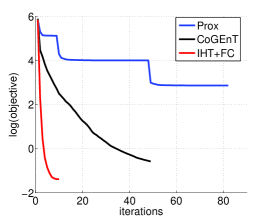
Refer to caption
Figure 3: Wavelet Transform recovery of 1-D test signals. (Left) The ‘blocks’ signal and recovery using IHT ++ Greedy projections. (Right) Objective function vs iterations on the ‘blocks’ signal.