Determination of intrinsic lifetime of edge magnetoplasmons

Abstract

It is known that peculiar plasmons whose frequencies are purely imaginary exist in the interior of a two-dimensional electronic system described by the Drude model. We show that when an external magnetic field is applied to the system, these bulk plasmons are still non-oscillating and are isolated from the magnetoplasmons by the energy gap of the cyclotron frequency. These are mainly in a transverse magnetic mode and can combine with a transverse electronic mode locally at an edge of the system to form edge magnetoplasmons. With this observation, we reveal the intrinsic long lifetime of edge magnetoplasmons for the first time.

Many types of intriguing phenomena can emerge at the edge of a material that are invisible or hiding in the interior for some reason. Edge magnetoplasmon is such an example; it is a gapless collective excitation that appears at the edge of a two-dimensional electron gas (2DEG) under the application of an external magnetic field. Allen et al. (1983); Glattli et al. (1985); Grodnensky et al. (1991); Ashoori et al. (1992); Tonouchi et al. (1994); Yan et al. (2012); Petković et al. (2013); Kumada et al. (2013) The properties unique to the edge magnetoplasmons, such as the localization length and dispersion relation, were calculated by Volkov and Mikhailov. Volkov and Mikhailov (1988) They succeeded in solving an integral equation of the electric potential using the Wiener-Hopf method. Noble (1958); Fetter (1985) Meanwhile, an internal magnetic field, which is coupled to the potential through Maxwell equations, is neglected, and this simplification prevents the lifetime of the edge magnetoplasmon ($\tau^{*}$ in Ref. Volkov and Mikhailov, 1988) from being determined and also obscures the magnetic configurations of the excitations. The fact that the localization length and dispersion relation are dependent on the lifetime makes it difficult to analyze experimental results.

In this paper, we determine the intrinsic lifetime of the edge magnetoplasmon. Our analyses are based on two observations. The first is that there is a purely relaxational state with a very long lifetime in the interior of a 2DEG. The second is that the state acquires a non-zero real part of the frequency through localization and starts to propagate. By showing that the properties of the localized state are consistent with those of the edge magnetoplasmons, we identified the purely relaxational state as the bulk counterpart of the edge magnetoplasmons and determined the lifetime of the edge magnetoplasmons. Our results show that the internal magnetic field normal to the layer is strongly suppressed in the interior, which partly justifies the assumption used in the past and may lead us to a more complete description of the edge magnetoplasmons.

We begin by reviewing a mathematical treatment of plasmons. The fact that magnetic fields are discontinuous at a 2DEG layer plays a central role in the formation of localized surface plasmons. Nakayama (1974); Chiu and Quinn (1974) The plasmons are classified into transverse magnetic (TM) and transverse electric (TE) modes with respect to their eigenvectors, as shown in Fig. 1. The electric fields of these eigenmodes are written in terms of the localization length in the direction normal to the layer $\alpha^{-1}$, in-plane wavevector $k_{y}$, and angular frequency $\omega$ as

$$\begin{split}&E_{x}=E^{\rm TE}_{x0}e^{i(k_{y}y-\omega t)}e^{-\alpha|z|},\\ &E_{y}=E^{\rm TM}_{y0}e^{i(k_{y}y-\omega t)}e^{-\alpha|z|},\\ &E_{z}=E^{\rm TM}_{z0}e^{i(k_{y}y-\omega t)}e^{-\alpha|z|},\end{split}$$ (1)

where $E^{\rm TE}_{x0}$ ($E^{\rm TM}_{y0}$ and $E^{\rm TM}_{z0}$) is the amplitude of the TE (TM) mode. Note that the $E_{i}$ values in Eq. (1) are proportional to $e^{-\alpha z}$ ($e^{+\alpha z}$) for $z>0$ ($z<0$). Note also that for $z<0$ we need to replace $E_{z}$ with $-E_{z}$ because Gauss’s law for free space, $\nabla\cdot{\bf E}=0$, must be satisfied for both $z>0$ and $z<0$. The magnetic fields are obtained from Eq. (1) using Faraday’s law, $\nabla\times{\bf E}=-\partial{\bf B}/\partial t$. For $z>0$, we have

$$\begin{split}&i\omega B_{x}=ik_{y}E_{z}+\alpha E_{y},\\ &i\omega B_{y}=-\alpha E_{x},\\ &i\omega B_{z}=-ik_{y}E_{x}.\end{split}$$ (2)

For $z<0$, we replace $\alpha$ and $E_{z}$ on the right-hand side of Eq. (2) with $-\alpha$ and $-E_{z}$, respectively. As a result, $B_{x}$ and $B_{y}$ are discontinuous at $z=0$ as shown in Fig. 1. By applying Stokes’ theorem to Ampére’s circuital law of the Maxwell equations, $c^{2}\nabla\times{\bf B}=\varepsilon\partial{\bf E}/\partial t+{\bf j}/\epsilon_{0}$ where ${\bf j}=(j_{x},j_{y},0)\delta(z)$ is the electronic current flowing in a layer, we find that the discontinuity of $B_{x}$ is related to $j_{y}$ as $c^{2}(B_{x}(z=0+)-B_{x}(z=0-))=j_{y}/\epsilon_{0}$. Because of Ohm’s law, ${\bf j}$ (on the right-hand side) is proportional to the in-plane electric fields as $j_{i}=\sigma_{ix}(\omega)E_{x}|_{z=0}+\sigma_{iy}(\omega)E_{y}|_{z=0}$ with the coefficients of the dynamical conductivity tensor $\sigma_{ij}(\omega)$ given below.  By applying a similar argument for $B_{y}$, we obtain the equations for the amplitudes,

$$\begin{pmatrix}\frac{2\alpha}{i\omega\mu_{0}}-\sigma_{xx}(\omega)&-\sigma_{xy}(\omega)\cr\sigma_{xy}(\omega)&\frac{2i\omega\epsilon}{\alpha}-\sigma_{xx}(\omega)\end{pmatrix}\begin{pmatrix}E^{\rm TE}_{x0}\cr E^{\rm TM}_{y0}\end{pmatrix}=0.$$ (3)

Here, $\mu_{0}$ ($\epsilon_{0}$) is the permeability (permittivity) of free space,

$$\alpha=\sqrt{k_{y}^{2}-\varepsilon\frac{\omega^{2}}{c^{2}}},$$ (4)

and $\varepsilon\equiv\epsilon/\epsilon_{0}$ is the relative permittivity of the surrounding material. We assume that $\varepsilon$ is a frequency-independent constant throughout this paper. A detailed derivation of Eqs. (3) and (4) is given in Appendix.

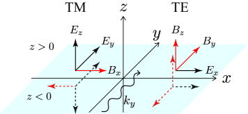
Figure 1: (color online) The electromagnetic fields (${\bf E}$ and ${\bf B}$) of the transverse magnetic (TM) and transverse electric (TE) modes are shown for $z>0$ (solid arrows) and $z<0$ (dashed). The discontinuities of $B_{x}$ ($E_{z}$) and $B_{y}$ at $z=0$ are relevant to the TM and TE modes, respectively. In contrast to $E_{z}$, $B_{z}$ cannot be discontinuous at $z=0$ because of the absence of a magnetic monopole. A 2DEG layer at $z=0$ is expressed by a transparent sheet.

We adopt the Drude model to calculate $\sigma_{ij}(\omega)$. The model describes the motion of an electron accelerated by the electric fields in an applied static magnetic field, ${\bf B}_{a}$. This motion is governed by the classical equation of motion: $m(d{\bf v}/dt+{\bf v}/\tau)=-e({\bf E}+{\bf v}\times{\bf B}_{a})$, where $m$ is the effective mass of the electron, $\tau$ is the relaxation time, and ${\bf v}$ is the velocity. The solution of the equation gives, with the definition of the current ${\bf j}\equiv-en{\bf v}$ ($n$ is the carrier density), the conductivities of the Drude model as

$$\begin{split}&\sigma_{xx}(\omega)=\frac{(1-i\omega\tau)\sigma_{0}}{(1-i\omega\tau)^{2}+(\omega_{c}\tau)^{2}},\\ &\sigma_{xy}(\omega)=-\frac{(\omega_{c}\tau)\sigma_{0}}{(1-i\omega\tau)^{2}+(\omega_{c}\tau)^{2}},\end{split}$$ (5)

where $\sigma_{0}=ne^{2}\tau/m$ is the static conductivity and $\omega_{c}=eB_{az}/m$ is the cyclotron frequency. The frequency and eigenvector of the surface plasmons are determined from Eq. (3) with Eq. (5).

It has been shown by Fal’ko and Khmel’nitskii that plasmons whose frequencies have no real part exist when $\omega_{c}=0$. Fal’ko and Khmel’nitskii (1989) The off-diagonal terms of Eq. (3) disappear, so that the TM and TE modes are decoupled completely. The TM mode satisfies the quadratic equation with respect to $\omega$,

$$\frac{2i\omega\epsilon}{\alpha}-\frac{\sigma_{0}}{1-i\omega\tau}=0.$$ (6)

In particular, when $\tau\ll\epsilon/2\sigma_{0}\alpha$, we obtain two roots corresponding to a long-lived mode with $\omega\simeq-i\sigma_{0}|k_{y}|/2\epsilon$ and a short-lived mode with $\omega\simeq-i/\tau$.  The frequencies of these modes have a zero real part and are expressed as $\omega=-i\delta$ with a positive real number $\delta$. The time evolution exhibits an exponential decay (overdamped oscillation), $e^{-i\omega t}=e^{-\delta t}$, in other words, they are non-oscillating and purely relaxational states. For the short-lived mode, the lifetime is identical to the relaxation time of the electron, suggesting that the mode is controlled by the electron’s motion. The lifetime of the long-lived mode is inversely proportional to $\tau$ since $\sigma_{0}$ is proportional to $\tau$ and is enhanced in the long-wavelength limit $|k_{y}|\to 0$.  These purely relaxational states are distinct from the mode extensively discussed in the literature that appears in the collisionless limit $\tau\gg\epsilon/2\sigma_{0}\alpha$. Stern (1967); Chaplik (1972); Wunsch et al. (2006); Hwang and Das Sarma (2007); Sasaki and Kumada (2014) The mode oscillates with the frequency,

$$\omega\simeq\pm\omega_{p}-\frac{i}{2\tau},$$ (7)

where

$$\omega_{p}\equiv\sqrt{\frac{\sigma_{0}\alpha}{2\epsilon\tau}}.$$ (8)

The positive frequency mode represents a propagating wave with a positive (negative) velocity in the direction of $y$ for $k_{y}>0$ ($k_{y}<0$). The negative frequency mode is an unphysical mode and should be omitted.

Whereas, a TE mode satisfies

$$\frac{2\alpha}{i\omega\mu_{0}}-\frac{\sigma_{0}}{1-i\omega\tau}=0.$$ (9)

This equation has a unique solution exhibiting an overdamped oscillation,

$$\omega=-\frac{i}{\tau+\frac{\sigma_{0}\mu_{0}}{2|k_{y}|}}.$$ (10)

The lifetime of the TE mode is enhanced in the long-wavelength limit $|k_{y}|\to 0$. On the other hand, the equation does not admit an underdamped oscillation with a non-zero real part of the frequency.

Figure 2: (color online) The existence of three branches of magnetoplasmons is shown by flows with circles in the complex $\omega$-plane. The axes are expressed in units of ps^-1. The arrows denote the directions of the change in frequency as the magnetic field or $\omega_{c}$ increases from $10^{11}$ to $3\times 10^{13}$ s^-1. We assumed that $\tau=1$ ps, $\alpha=1\mu$m^-1, $\sigma_{0}=10^{-3}$ $\Omega^{-1}$, and $\varepsilon=2.4$. The lifetime of the (bulk) magnetoplasmons in the high magnetic field limit corresponds to the value of $\tau$.

The system supports three eigenmodes in the presence of an external magnetic field. This is because we obtain the cubic equation with respect to $\omega$, by making the determinant of the matrix of Eq. (3) equal to zero, as

$$\frac{4\epsilon}{\mu_{0}}\left\{(1-i\omega\tau)^{2}+(\omega_{c}\tau)^{2}\right\}$$

$$-(1-i\omega\tau)\sigma_{0}\left(\frac{2i\omega\epsilon}{\alpha}+\frac{2\alpha}{i\omega\mu_{0}}\right)+\sigma_{0}^{2}=0.$$ (11)

The $\omega$ values of three solutions, which are calculated numerically, are shown in the complex $\omega$-plane in Fig. 2 for the typical case of parameters. We find that the system supports a purely relaxational state in the presence of an external magnetic field. The frequency is found analytically when $\tau$ is sufficiently large ($|\omega_{c}|\tau\gg 1$) as

$$\omega\simeq-\frac{i}{\tau+\frac{\omega_{c}^{2}}{\omega_{p}^{2}}\tau+\frac{\mu_{0}\sigma_{0}}{2\alpha}}.$$ (12)

The lifetime of this purely relaxational state is elongated by increasing $|\omega_{c}|$ or in the long-wavelength limit. The eigenvector is dominated by the TM component when $\sigma_{0}/\epsilon_{0}c\ll(|\omega_{c}|\tau)^{3/2}$ is satisfied. The dominance of the TM component is slightly peculiar because Eq. (12) reproduces the frequency of the TE mode Eq. (10) in the limit $\omega_{c}=0$. The purely relaxational state is distinct from the bulk magnetoplasmons with respect to the positions in the frequency domain and eigenvectors. The dispersion relation of the bulk magnetoplasmons is obtained by making the component that is proportional to $\epsilon\tau^{2}/\mu_{0}$ in Eq. (11) equal to zero as Chiu and Quinn (1974)

$$\omega_{mp}(\omega_{c})=\pm\sqrt{\omega_{c}^{2}+\omega_{p}^{2}}-\frac{i}{\tau}.$$ (13)

The negative frequency mode is an unphysical mode that should be omitted. The eigenvectors of the modes are a hybrid of the TM and TE modes. Generally, they are categorized as an elliptical polarization. Practically, they are linear polarization because the TE component is dominant in a strong magnetic field ($\sigma_{xy}\gg\sigma_{xx}$).

It can be shown that the non-oscillating state found above starts oscillating when the state is localized. We consider localized electric fields of the form,

$$\begin{split}&E_{x}=E_{x0}e^{i(k_{y}y-\omega t)}e^{-\beta x}e^{-\alpha|z|},\\ &E_{y}=E_{y0}e^{i(k_{y}y-\omega t)}e^{-\beta x}e^{-\alpha|z|},\\ &E_{z}=E_{z0}e^{i(k_{y}y-\omega t)}e^{-\beta x}e^{-\alpha|z|}.\end{split}$$ (14)

Here $\beta^{-1}$ is the lateral localization length from an edge and, if $\beta=0$, the electric fields reproduce Eq. (1). For the moment, we consider a positive $\beta$ by limiting our attention to the bulk of the right half-plane of $x>0$. Using the Maxwell equations (see Appendix for detailed derivations), we obtain a generalized version of Eq. (3) with a modified 2$\times$2 matrix of the form:

$$\begin{pmatrix}\frac{2\alpha}{i\omega\mu_{0}}\left(1+\frac{\beta^{2}}{\alpha^{2}}\right)-\sigma_{xx}(\omega)&-\frac{2k_{y}}{\omega\mu_{0}}\frac{\beta}{\alpha}-\sigma_{xy}(\omega)\cr-\frac{2k_{y}}{\omega\mu_{0}}\frac{\beta}{\alpha}+\sigma_{xy}(\omega)&\frac{2i\omega\epsilon}{\alpha}-\sigma_{xx}(\omega)-\frac{2\beta}{i\omega\mu_{0}}\frac{\beta}{\alpha}\end{pmatrix}.$$ (15)

Each element of this matrix contains a term that is proportional to $\omega^{-1}$, which is enhanced for the solution of Eq. (12) because the $\omega$ is very close to the origin of the complex $\omega$-plane.  This suggests that the eigenvector is modified accordingly so that the term is suppressed. From Eq. (15) the condition on the eigenvector is read off as

$$\frac{\beta E_{y0}+ik_{y}E_{x0}}{i\omega}=0,$$ (16)

which is equivalent to an internal magnetic field $B_{z}$ being suppressed in the bulk (see Eq. (23)).  By using Eq. (16), we have the equations for the amplitudes as follows:

$$\begin{pmatrix}\frac{2\alpha}{i\omega\mu_{0}}\left(1+\frac{\beta^{2}}{\alpha^{2}}\right)-\sigma_{xx}(\omega)&-\frac{2k_{y}}{\omega\mu_{0}}\frac{\beta}{\alpha}-\sigma_{xy}(\omega)\cr\sigma_{xy}(\omega)&\frac{2i\omega\epsilon}{\alpha}-\sigma_{xx}(\omega)\end{pmatrix}\begin{pmatrix}E_{x0}\cr E_{y0}\end{pmatrix}=0.$$ (17)

The vanishing determinant of the $2\times 2$ matrix in Eq. (17) leads to the following cubic equation with respect to $\omega$:

$$\omega_{c}^{2}+\omega_{p}^{2}-\omega^{2}-\frac{i\omega\mu_{0}\sigma_{0}}{2\alpha(1+\frac{\beta^{2}}{\alpha^{2}})\tau^{2}}$$

$$+\frac{\sigma_{0}\mu_{0}}{2\tau\alpha}\frac{\omega_{p}^{2}-\omega^{2}}{1+\frac{\beta^{2}}{\alpha^{2}}}-\frac{\omega_{p}^{2}}{i\omega\tau}-\frac{\omega_{c}}{\omega}\frac{\omega_{p}^{2}\beta k_{y}}{\alpha^{2}+\beta^{2}}=0.$$ (18)

There is a solution that is approximated as

$$\omega\simeq\frac{\omega_{p}^{2}}{\omega_{c}}\frac{\beta}{\alpha^{2}+\beta^{2}}k_{y}-\frac{i}{\tau+\frac{\omega_{c}^{2}}{\omega_{p}^{2}}\tau+\frac{\mu_{0}\sigma_{0}}{2\alpha(1+\frac{\beta^{2}}{\alpha^{2}})}}.$$ (19)

The frequency has a non-zero real part, which is linear in $k_{y}$. The fact that ${\rm Re}(\omega)/k_{y}\propto 1/\omega_{c}$ shows that the mode is chiral (propagation direction is dependent on the sign of $B_{az}$). Note also that the group velocity is suppressed when $|\omega_{c}|$ is increased and the localization length $\beta^{-1}$ is fixed. All these properties of this solution are consistent with those of the edge magnetoplasmons and Eq. (19) can reproduce Eq. (12) in the $\beta=0$ limit. Thus, we identify the mode with the edge magnetoplasmons. It is worth noting that the intrinsic decay time of an edge magnetoplasmon is derived from Eq. (19) as

$$\tau_{emp}\simeq\frac{\omega_{c}^{2}+\omega_{p}^{2}}{\omega_{p}^{2}}\tau,$$ (20)

where $\mu_{0}\sigma_{0}/2\alpha(1+\frac{\beta^{2}}{\alpha^{2}})$ is omitted. The ratio of $\tau_{emp}$ to $\tau$ increases as $|B_{az}|$ increases, and it is expressed in terms of the angular frequencies of the magnetoplasmons as $\tau_{emp}/\tau=\omega^{2}_{mp}(\omega_{c})/\omega^{2}_{mp}(0)$. Note that $\tau$ can depend on $|B_{az}|$, and the dependence can be determined from the lifetime of the magnetoplasmons (see Eq. (13)). 

Equation (20) can be used to explain a recent experiment on the edge magnetoplasmons in graphene reported by Yan et al. Yan et al. (2012). In Fig. 3, magnetic field dependences of the full width at half maximum (FWHM) of bulk and edge magnetoplasmons are indicated by errorbars with filled and empty squares, respectively. These are the experimental data taken from Fig. 2(D) in Ref. Yan et al., 2012. The plot of $2/c\tau_{emp}$ gives errorbars with circles, where $\tau$ in Eq. (20) is taken from the experiment (the errorbars with filled squares).  The close agreement between the positions of circles and empty squares supports the validity of our result. Moreover, $\tau_{emp}$ is elongated by decreasing $|k_{y}|$ through $\omega_{p}$, which is consistent with a recent experiment on the dissipation mechanism in graphene. Kumada et al. (2014)

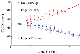
Figure 3: (color online) Equation (20) is applied to a recent experiment on the edge magnetoplasmons in graphene reported by Yan et al. Yan et al. (2012) The close agreement between the circle and empty square plots supports the validity of Eq. (20). The dashed curves are the plots of $69\sqrt{(\omega_{c}^{2}+\omega_{p}^{2})/\omega_{p}^{2}}$ cm^-1 and $69\sqrt{\omega_{p}^{2}/(\omega_{c}^{2}+\omega_{p}^{2})}$ cm^-1. The errorbars with circles are shifted slightly horizontally from the proper values of the magnetic field in order to avoid overlap between the plots.

Our derivation of the intrinsic lifetime of the edge magnetoplasmons does not assume the details of the boundary of a 2DEG and therefore has a wide application. This is in contrast to the analyses of Volkov and Mikhailov, in which a sharp electron density profile at the boundary (sharp edge) is assumed. The edges of graphene and InAs meet this assumption, while GaAs might not because of the existence of a depletion layer several micrometers thick. Acoustic types of edge magnetoplasmons have been predicted for such smooth edge. Aleiner and Glazman (1994) Note that since plasmon is the hybrid of electrons and electromagnetic fields, it is difficult to identify the lifetime of edge magnetoplasmon with the lifetime of electrons at only the edge channel. Our formulation does not assume the specific properties of the electric edge states, such as the absence of back scattering, but it yields close agreement between Eq. (20) and the result in Ref. Yan et al., 2012. This fact suggests that because the experiment by Yan et al. Yan et al. (2012) is performed in the classical Hall effect region, many electronic states including not only the edge states but also (bulk) states near the edge (up to several micrometers from the edge) are participating in the dynamics of the edge magnetoplasmon. The present model suggests an intriguing physical interpretation of the longer lifetime based on the hybridization of the TE and TM modes. A deviation from Eq. (20) may appear in the quantum Hall effect region and it can be attributed to the contribution of the specific properties of the electric edge states.

Figure 4: (color online) (a) The magnetic field of a purely relaxational TM dominant state with $\beta=0$ is shown for $z>0$ and $z<0$. The sheet current $j_{y}\delta(z)$ that causes the discontinuity of $B_{x}$, is represented by a transparent layer. (b) When we introduce the edge along the $y$-axis, the magnetic fields at $z>0$ and $z<0$ must combine. The magnetic field at the edge has a non-zero $z$-component, which is a locally induced TE mode. (c) The edge-induced hybridization of the TE and TM modes results in an edge magnetoplasmon with a chiral propagation property.

The finite real part of the frequency of an edge magnetoplasmon originates from the mixing of $E_{x0}$ and $E_{y0}$. Namely, when we make a purely relaxational state localized by a non-zero $\beta$, the eigenvector of the state is modified according to $\beta E_{y0}+ik_{y}E_{x0}=0$ for $x>0$. An important feature of the modified eigenvector for $x<0$, for which $\beta E_{y0}+ik_{y}E_{x0}=0$ does not need to be satisfied, can be grasped pictorially without a mathematical calculation. Suppose that as shown in Fig. 4(a), a purely relaxational state, which is a TM dominant mode, exists for a finite period of time in a periodic system without an edge. Note that the magnetic field $B_{x}$ at $z=0+$ is pointing in the opposite direction to that at $z=0-$. If we introduce the edge along the $y$-axis (by cutting the layer) in Fig. 4(b), the magnetic fields at $z>0$ and $z<0$ must combine and form a closed curve to satisfy one of the Maxwell equations: $\nabla\cdot{\bf B}=0$. Thus, the magnetic field must have a non-zero $z$-component at the edge, which is a locally induced TE mode.  We may regard the edge magnetoplasmon as a composite of the TE mode at the edge and the spatially decaying TM mode in the bulk, as shown in Fig. 4(c).

Since a TE mode is inevitably hybridized with the purely relaxational state when the state changes into an edge magnetoplasmon, the fact that a TE mode exhibits anomalous behavior in graphene is noteworthy. Mikhailov and Ziegler pointed out that the imaginary part of the dynamical conductivity of graphene can be negative for a specific frequency, Mikhailov and Ziegler (2007) because an interband transition contributes to the dynamical conductivity, while the Drude model only accounts for an intraband transition. As a result, they predict that graphene can support a TE mode for a special frequency (even without an external magnetic field). We can easily see from Eq. (9) that an oscillating TE mode can appear when the imaginary part of the dynamical conductivity is a negative number. Bordag and Pirozhenko argued that the existence of an infinitesimal mass gap in graphene leads to a special TE mode that propagates at the speed of light. Bordag and Pirozhenko (2014)

In summary, the peculiarities of a purely relaxational state in the bulk are partly eliminated by knowing their relationship to edge magnetoplasmons, which have constituted the theme of various published reports. Allen et al. (1983); Glattli et al. (1985); Grodnensky et al. (1991); Ashoori et al. (1992); Tonouchi et al. (1994); Yan et al. (2012); Petković et al. (2013); Kumada et al. (2013) The strange behavior found for the state, such as the intrinsic long lifetime being proportional to the square of the applied magnetic field, is our original conclusion that has not been taken into account before. Our result whereby the eigenvector is TM dominant with a very long-lived $E_{z}$ component has an advantage in that it detects the signal via an electrode in a transient manner.  The local mixing with the TE mode may also imply that ferromagnetic electrodes can excite the edge magnetoplasmons.

Appendix A Derivation of Eq. (17)

By applying Faraday’s law to the electric fields Eq. (14), we obtain the magnetic fields for $z>0$ as

$$i\omega B_{x}=ik_{y}E_{z}+\alpha E_{y},$$ (21)

$$i\omega B_{y}=-\alpha E_{x}+\beta E_{z},$$ (22)

$$i\omega B_{z}=-\beta E_{y}-ik_{y}E_{x}.$$ (23)

For $z<0$, the magnetic fields are given by replacing $\alpha$ with $-\alpha$ and $E_{z}$ with $-E_{z}$ on the right-hand side. As a result, $B_{x}$ and $B_{y}$ change their signs at $z=0$. Note that the sign change of $E_{z}$ imposed at $z=0$ is still consistent with Gauss’s law, which gives

$$-\beta E_{x}+ik_{y}E_{y}-\alpha E_{z}=0.$$ (24)

It is useful to write Eqs. (21), (22), and (23) in the form of a $3\times 3$ matrix as $i\omega{\bf B}=M{\bf E}$ where ${\bf E}={}^{t}(E_{x},E_{y},E_{z})$, ${\bf B}={}^{t}(B_{x},B_{y},B_{z})$, and

$$M=\begin{pmatrix}0&\alpha&ik_{y}\cr-\alpha&0&\beta\cr-ik_{y}&-\beta&0\end{pmatrix}.$$ (25)

By applying Ampére’s circuital law for free space ($z\neq 0$) where the charged current is absent (${\bf j}=0$), $c^{2}\nabla\times{\bf B}=\varepsilon\partial{\bf E}/\partial t$ , we obtain

$$\left(\frac{-i\omega\varepsilon}{c^{2}}\right){\bf E}=M{\bf B}.$$ (26)

By multiplying $i\omega$ with both sides and using $i\omega{\bf B}=M{\bf E}$, we have $[\varepsilon\frac{\omega^{2}}{c^{2}}-M^{2}]{\bf E}=0$. Thus, a non-vanishing electric field is possible when ${\rm det}[\varepsilon\frac{\omega^{2}}{c^{2}}-M^{2}]=0$, namely, when

$$\varepsilon\omega^{2}\left(-k_{y}^{2}+\alpha^{2}+\beta^{2}+\frac{\varepsilon\omega^{2}}{c^{2}}\right)^{2}=0$$ (27)

is satisfied.

The boundary conditions for the magnetic fields $B_{x}$ and $B_{y}$ at $z=0$ are expressed by

$$c^{2}\left(B_{y}(z=0_{-})-B_{y}(z=0_{+})\right)=\frac{j_{x}(x,y)}{\epsilon_{0}},$$ (28)

$$c^{2}\left(B_{x}(z=0_{+})-B_{x}(z=0_{-})\right)=\frac{j_{y}(x,y)}{\epsilon_{0}}.$$ (29)

Putting Eqs. (21) and (22) into these boundary conditions and using Eqs. (23), (24), and (27), we obtain Eq. (15) or

$$\begin{pmatrix}\frac{2\alpha}{i\omega\mu_{0}}\left(1+\frac{\beta^{2}}{\alpha^{2}}\right)-\sigma_{xx}(\omega)&-\frac{2k_{y}}{\omega\mu_{0}}\frac{\beta}{\alpha}-\sigma_{xy}(\omega)\cr-\frac{2k_{y}}{\omega\mu_{0}}\frac{\beta}{\alpha}+\sigma_{xy}(\omega)&\frac{2i\omega\epsilon}{\alpha}-\sigma_{xx}(\omega)-\frac{2\beta}{i\omega\mu_{0}}\frac{\beta}{\alpha}\end{pmatrix}\begin{pmatrix}E_{x0}\cr E_{y0}\end{pmatrix}=0.$$ (30)

This equation reproduces Eq. (17) when

$$\frac{\beta E_{y0}+ik_{y}E_{x0}}{i\omega}=0.$$ (31)

It is noted that the determinant of the matrix of Eq. (30) is independent of the variable $\beta$. Indeed, by setting $\beta=-ik_{x}$ in Eq. (14), it is easily understood that the inclusion of $\beta$ merely changes the propagation direction. Thus, the solutions are given by Eqs. (12) and (13), and therefore Eq. (30) fails to reproduces the edge magnetoplasmons. This clarifies the importance of the condition Eq. (31).

It is possible to estimate the value of $\beta$ using Eq. (31). By putting the eigenstate of Eq. (17) on Eq. (31), we obtain

$$\beta\simeq\frac{k_{y}}{\omega_{c}}\left(1+\frac{\omega_{c}^{2}}{\omega_{p}^{2}}\right)\omega+i\frac{k_{y}}{\omega_{c}\tau},$$ (32)

which is correct up to the first order of $\omega$. By substituting Eq. (19) for $\omega$, we obtain

$$\alpha^{2}+\beta^{2}\simeq\frac{\omega_{c}^{2}+\omega_{p}^{2}}{\omega_{c}^{2}}k_{y}^{2}.$$ (33)

Thus, $\beta$ is determined as a function of $\alpha$. We note that the $\alpha$ value is determined from $\omega_{p}$ or $\omega_{mp}(\omega_{c})$. It is also worth noting that with Eq. (32), we can obtain $\omega$ as a function of $\alpha$ by eliminating $\beta$ from Eq. (27). The calculated $\omega$ reproduces Eq. (19).

References

- Allen et al. (1983) S. J. Allen, H. L. Störmer, and J. C. M. Hwang, Physical Review B, 28, 4875 (1983), ISSN 0163-1829.
- Glattli et al. (1985) D. C. Glattli, E. Y. Andrei, G. Deville, J. Poitrenaud, and F. I. B. Williams, Physical Review Letters, 54, 1710 (1985), ISSN 0031-9007.
- Grodnensky et al. (1991) I. Grodnensky, D. Heitmann, and K. von Klitzing, Physical Review Letters, 67, 1019 (1991), ISSN 0031-9007.
- Ashoori et al. (1992) R. C. Ashoori, H. L. Stormer, L. N. Pfeiffer, K. W. Baldwin, and K. West, Physical Review B, 45, 3894 (1992), ISSN 0163-1829.
- Tonouchi et al. (1994) M. Tonouchi, T. Miyasato, P. Hawker, T. Cheng, and V. Rampton, Journal of the Physical Society of Japan, 63, 4499 (1994), ISSN 0031-9015.
- Yan et al. (2012) H. Yan, Z. Li, X. Li, W. Zhu, P. Avouris, and F. Xia, Nano letters, 12, 3766 (2012), ISSN 1530-6992.
- Petković et al. (2013) I. Petković, F. I. B. Williams, K. Bennaceur, F. Portier, P. Roche, and D. C. Glattli, Physical Review Letters, 110, 016801 (2013), ISSN 0031-9007.
- Kumada et al. (2013) N. Kumada, S. Tanabe, H. Hibino, H. Kamata, M. Hashisaka, K. Muraki, and T. Fujisawa, Nature communications, 4, 1363 (2013), ISSN 2041-1723.
- Volkov and Mikhailov (1988) V. A. Volkov and S. A. Mikhailov, Sov. Phys. JETP, 67, 1639 (1988).
- Noble (1958) B. Noble, Methods based on the Wiener-Hopf technique for the solution of partial differential equations (Pergamon Press, 1958).
- Fetter (1985) A. Fetter, Physical Review B, 32, 7676 (1985), ISSN 0163-1829.
- Nakayama (1974) M. Nakayama, J. Phys. Soc. Jpn., 36, 393 (1974).
- Chiu and Quinn (1974) K. W. Chiu and J. J. Quinn, Physical Review B, 9, 4724 (1974), ISSN 0556-2805.
- Fal’ko and Khmel’nitskii (1989) V. Fal’ko and D. Khmel’nitskii, Sov. Phys. JETP, 68, 1150 (1989).
- Stern (1967) F. Stern, Physical Review Letters, 18, 546 (1967), ISSN 0031-9007.
- Chaplik (1972) A. Chaplik, Sov. Phys. JETP, 35, 395 (1972).
- Wunsch et al. (2006) B. Wunsch, T. Stauber, F. Sols, and F. Guinea, New Journal of Physics, 8, 318 (2006), ISSN 1367-2630.
- Hwang and Das Sarma (2007) E. H. Hwang and S. Das Sarma, Physical Review B, 75, 205418 (2007), ISSN 1098-0121.
- Sasaki and Kumada (2014) K.-i. Sasaki and N. Kumada, Physical Review B, 90, 035449 (2014), ISSN 1098-0121.
- Kumada et al. (2014) N. Kumada, P. Roulleau, B. Roche, M. Hashisaka, H. Hibino, I. Petković, and D. C. Glattli, Physical Review Letters, 113, 266601 (2014), ISSN 0031-9007.
- Aleiner and Glazman (1994) I. Aleiner and L. Glazman, Physical Review Letters, 72, 2935 (1994), ISSN 0031-9007.
- Mikhailov and Ziegler (2007) S. Mikhailov and K. Ziegler, Physical Review Letters, 99, 016803 (2007), ISSN 0031-9007.
- Bordag and Pirozhenko (2014) M. Bordag and I. G. Pirozhenko, Physical Review B, 89, 035421 (2014), ISSN 1098-0121.