ABRA: Approximating Betweenness Centrality
in Static and Dynamic Graphs with Rademacher Averages

Abstract

We present ABRA, a suite of algorithms that compute and maintain probabilistically-guaranteed, high-quality, approximations of the betweenness centrality of all nodes (or edges) on both static and fully dynamic graphs. Our algorithms rely on random sampling and their analysis leverages on Rademacher averages and pseudodimension, fundamental concepts from statistical learning theory. To our knowledge, this is the first application of these concepts to the field of graph analysis. The results of our experimental evaluation show that our approach is much faster than exact methods, and vastly outperforms, in both speed and number of samples, current state-of-the-art algorithms with the same quality guarantees.

ΑΒΡΑΞΑΣ (ABRAXAS): Gnostic word of mystic meaning

1 Introduction

Centrality measures are fundamental concepts in graph analysis, as they assign to each node or edge in the network a score that quantifies some notion of importance of the node/edge in the network [28]. Betweenness Centrality (bc) is a very popular centrality measure that, informally, defines the importance of a node or edge $z$ in the network as proportional to the fraction of shortest paths in the network that go through $z$ [2, 16].

Brandes [12] presented an algorithm (denoted BA) that computes the exact bc values for all nodes or edges in a graph $G=(V,E)$ in time $O(|V||E|)$ if the graph is unweighted, and time $O(|V||E|+|V|^{2}\log|V|)$ if the graph has positive weights. The cost of BA is excessive on modern networks with millions of nodes and tens of millions of edges. Moreover, having the exact bc values may often not be needed, given the exploratory nature of the task, and a high-quality approximation of the values is usually sufficient, provided it comes with stringent guarantees.

Today’s networks are not only large, but also dynamic: edges are added and removed continuously. Keeping the bc values up-to-date after edge insertions and removals is a challenging task, and proposed algorithms [23, 18, 22, 24] have a worst-case complexity and memory requirements which is not better than from-scratch-recomputation using BA. Maintaining an high-quality approximation up-to-date is more feasible and more sensible: there is little added value in keeping track of exact bc values that change continuously.

Contributions

We focus on developing algorithms for approximating the bc of all vertices and edges in static and dynamic graphs. Our contributions are the following.

• We present ABRA (for “Approximating Betweenness with Rademacher Averages”), the first family of algorithms based on progressive sampling for approximating the bc of all vertices in static and dynamic graphs, where vertex and edge insertions and deletions are allowed. The approximations computed by ABRA are probabilistically guaranteed to be within an user-specified additive error from their exact values. We also present variants with relative (i.e., multiplicative)) error for the top-$k$ vertices with highest bc, and variants that use refined estimators to give better approximations with a slightly larger sample size.

• Our analysis relies on Rademacher averages [34] and pseudodimension [30], fundamental concepts from the field of statistically learning theory [36]. Exploiting known and novel results using these concepts, ABRA computes the approximations without having to keep track of any global property of the graph, in contrast with existing algorithms [31, 7, 9]. ABRA performs only “real work” towards the computation of the approximations, without having to compute such global properties or update them after modifications of the graph. To the best of our knowledge, ours is the first application of Rademacher averages and pseudodimension to graph analysis problems, and the first to use progressive random sampling for bc computation. Using pseudodimension new analytical results on the sample complexity of the bc computation task, generalizing previous contributions [31], and formulating a conjecture on the connection between pseudodimension and the distribution of shortest path lengths.

• The results of our experimental evaluation on real networks show that ABRA outperforms, in both speed and number of samples, the state-of-the-art methods offering the same guarantees [31].

Outline

We discuss related works in Sect. 2. The formal definitions of the concepts we use in the work can be found in Sect. 3. Our algorithms for approximating bc on static graphs are presented in Sect. 4, while the dynamic case is discussed in Sect. 5. The results of our extensive experimental evaluation are presented in Sect. 6. We draw conclusions and outline directions for future work in Sect. 7. Additional details can be found in the Appendices.

2 Related Work

The definition of Betweenness Centrality comes from the sociology literature [2, 16], but the study of efficient algorithms to compute it started only when graphs of substantial size became available to the analysts, following the emergence of the Web. The BA algorithm by Brandes [12] is currently the asymptotically fastest algorithm for computing the exact bc values for all nodes in the network. A number of works also explored heuristics to improve BA [33, 15], but retained the same worst-case time complexity.

The use of random sampling to approximate the bc values in static graphs was proposed independently by Bader et al. [5] and Brandes and Pich [13], and successive works explored the tradeoff space of sampling-based algorithms [31, 7, 9, 8]. We focus here on related works that offer approximation guarantees similar to ours. For an in-depth discussion of previous contributions approximating bc on static graphs, we refer the reader to [31, Sect. 2].

Riondato and Kornaropoulos [31] present algorithms that employ the Vapnik-Chervonenkis (VC) dimension [36] to compute what is currently the tightest upper bound to the sample size sufficient to obtain guaranteed approximations of the bc of all nodes in a static graph. Their algorithms offer the same guarantees as ours, but they need to compute an upper bound to a characteristic quantity of the graph (the vertex diameter, namely the maximum number of nodes on any shortest path) in order to derive the sample size. Thanks to our use of Rademacher averages in a progressive random sampling setting, we do not need to compute any characteristic quantity of the graph, and instead use an efficient-to-evaluate stopping condition to determine when the approximated bc values are close to the exact ones. This allows ABRA to use smaller samples and be much faster than the algorithm by Riondato and Kornaropoulos [31].

A number of works [23, 18, 22, 24] focused on computing the exact bc for all nodes in a dynamic graph, taking into consideration different update models. None of these algorithm is provably asymptotically faster than a complete computation from scratch using Brandes’ algorithm [12] and they all require significant amount of space (more details about these works can be found in [7, Sect. 2]). In contrast, Bergamini and Meyerhenke [7, 8] built on the work by Riondato and Kornaropoulos [31] to derive an algorithm for maintaining high-quality approximations of the bc of all nodes when the graph is dynamic and both additions and deletions of edges are allowed. Due to the use of the algorithm by Riondato and Kornaropoulos [31] as a building block, the algorithm must keep track of the vertex diameter after an update to the graph. Our algorithm for dynamic graphs, instead, does not need this piece of information, and therefore can spend more time in computing the approximations, rather than in keeping track of global properties of the graph. Moreover, our algorithm can handle directed graphs, which is not the case for the algorithms by Bergamini and Meyerhenke [7, 8].

Hayashi et al. [21] recently proposed a data structure called Hypergraph Sketch to maintain the shortest path DAGs between pairs of nodes following updates to the graph. Their algorithm uses random sampling and this novel data structure allows them to maintain a high-quality, probabilistically guaranteed approximation of the bc of all nodes in a dynamic graph. Their guarantees come from an application of the simple uniform deviation bounds (i.e., the union bound) to determine the sample size, as previously done by Bader et al. [5] and Brandes and Pich [13]. As a result, the resulting sample size is excessively large, as it depends on the number of nodes in the graph. Our improved analysis using the Rademacher averages allows us to develop an algorithm that uses the Hypergraph Sketch with a much smaller number of samples, and is therefore faster.

3 Preliminaries

We now introduce the formal definitions and basic results that we use throughout the paper.

3.1 Graphs and Betweenness Centrality

Let $G=(V,E)$ be a graph, which can be directed or undirected, and can have non-negative weights on the edges. For any ordered pair $(u,v)$ of different nodes $u\neq v$, let $\mathcal{S}_{uv}$ be the set of Shortest Paths (SPs) from $u$ to $v$, and let $\sigma_{uv}=|\mathcal{S}_{uv}|$. Given a path $p$ between two nodes $u,v\in V$, a node $w\in V$ is internal to $p$ iff $w\neq u$, $w\neq u$, and $p$ goes through $w$. We denote as $\sigma_{uv}(w)$ the number of SPs from $u$ to $v$ that $w$ is internal to.

Definition 1 ([2, 16]).

Given a graph $G=(V,E)$, the Betweenness Centrality (bc) of a vertex $w\in V$ is defined as

$$\mathsf{b}(w)=\frac{1}{|V|(|V|-1)}\sum_{\begin{subarray}{c}(u,v)\in V\times V\\ u\neq v\end{subarray}}\frac{\sigma_{uv}(w)}{\sigma_{uv}}\enspace.$$

We have $\mathsf{b}(w)\in[0,1]$, for any $w\in V$. Many variants of bc have been proposed in the literature, including one for edges [28]. All our results can be extended to these variants, following the reduction in [31, Sect. 6], but we do not include them here due to space constraints.

In this work we focus on computing an $(\varepsilon,\delta)$-approximation of the collection $B=\{\mathsf{b}(w),w\in V\}$.

Definition 2.

Given $\varepsilon,\delta\in(0,1)$, an $(\varepsilon,\delta)$-approximation to $B$ is a collection $\tilde{B}=\{\tilde{\mathsf{b}}(w),w\in V\}$ such that

$$\Pr(\forall w\in v\leavevmode\nobreak\ :\leavevmode\nobreak\ |\tilde{\mathsf{b}}(w)-\mathsf{b}(w)|\leq\varepsilon)\geq 1-\delta\enspace.$$

3.2 Rademacher Averages

Rademacher Averages are fundamental concepts to study the rate of convergence of a set of sample averages to their expectations. They are at the core of statistical learning theory [36] but their usefulness extends way beyond the learning framework [32]. We present here only the definitions and results that we use in our work and we refer the readers to, e.g., the book by Shalev-Shwartz and Ben-David [34] for in-depth presentation and discussion.

While the Rademacher complexity can be defined on an arbitrary measure space, we restrict our discussion here to a sample space that consists of a finite domain $\mathcal{D}$ and a uniform distribution over that domain. Let $\mathcal{F}$ be a family of functions from $\mathcal{D}$ to $[0,1]$, and let $\mathcal{S}=\{c_{1},\dotsc,c_{\ell}\}$ be a sample of $\ell$ elements from $\mathcal{D}$, sampled uniformly and independently at random. For each $f\in\mathcal{F}$, the true sample and the sample average of $f$ on a sample $\mathcal{S}$ are

$$\mathsf{m}_{\mathcal{D}}(f)\frac{1}{|\mathcal{D}|}\sum_{c\in\mathcal{D}}^{\ell}f(c)\leavevmode\nobreak\ \leavevmode\nobreak\ \mbox{and}\leavevmode\nobreak\ \leavevmode\nobreak\ \mathsf{m}_{\mathcal{S}}(f)=\frac{1}{\ell}\sum_{i=1}^{\ell}f(c_{i}).$$ (1)

Given $\mathcal{S}$, we are interested in bounding the maximum deviation of $\mathsf{m}_{\mathcal{S}}(f)$ from $\mathsf{m}_{\mathcal{D}}(f)$, i.e., in the quantity

$$\sup_{f\in\mathcal{F}}|\mathsf{m}_{\mathcal{S}}(f)-\mathsf{m}_{\mathcal{D}}(f)|\enspace.$$ (2)

For $1\leq i\leq\ell$, let $\sigma_{i}$ be a Rademacher r.v., i.e., a r.v. that takes value $1$ with probability $1/2$ and $-1$ with probability $1/2$. The r.v.’s $\sigma_{i}$ are independent. Consider the quantity

$$\mathsf{R}(\mathcal{F},\mathcal{S})=\mathbb{E}_{\sigma}\left[\sup_{f\in\mathcal{F}}\frac{1}{\ell}\sum_{i=1}^{\ell}\sigma_{i}f(c_{i})\right],$$ (3)

where the expectation is taken w.r.t. the Rademacher r.v.’s, i.e., conditionally on $\mathcal{S}$. The quantity $\mathsf{R}(\mathcal{F},\mathcal{S})$ is known as the (conditional) Rademacher average of $\mathcal{F}$ on $\mathcal{S}$. The following is a key result in statistical learning theory, connecting $\mathsf{R}(\mathcal{F},\mathcal{S})$ to the maximum deviation (2).

Theorem 1 (Thm. 26.5 [34]).

Let $\delta\in(0,1)$ and let $\mathcal{S}$ be a collection of $\ell$ elements of $\mathcal{D}$ sampled independently and uniformly at random. Then, with probability at least $1-\delta$,

$$\sup_{f\in\mathcal{F}}|\mathsf{m}_{\mathcal{S}}(f)-\mathsf{m}_{\mathcal{D}}(f)|\leq 2\mathsf{R}(\mathcal{F},\mathcal{S})+3\sqrt{\frac{\ln(2/\delta)}{2\ell}}\enspace.$$ (4)

Thm. 1 is how the result is classically presented, but better although more complex bounds than (4) are available [29].

Theorem 2 (Thm. 3.11 [29]).

Let $\delta\in(0,1)$ and let $\mathcal{S}$ be a collection of $\ell$ elements of $\mathcal{D}$ sampled independently and uniformly at random. Let

$$\alpha=\frac{\ln\frac{2}{d}}{\ln\frac{2}{d}+\sqrt{\left(2\ell\mathsf{R}(\mathcal{F},\mathcal{S})+\ln\frac{2}{d}\right)\ln\frac{2}{d}}},$$ (5)

then, with probability at least $1-\delta$,

$$\sup_{f\in\mathcal{F}}|\mathsf{m}_{\mathcal{S}}(f)-\mathsf{m}_{\mathcal{D}}(f)|\leq\frac{\mathsf{R}(\mathcal{F},\mathcal{S})}{1-\alpha}+\frac{\ln\frac{2}{d}}{2\ell\alpha(1-\alpha)}+\sqrt{\frac{\ln\frac{2}{d}}{2\ell}}\enspace.$$ (6)

Computing, or even estimating, the expectation in (3) w.r.t. the Rademacher r.v.’s is not straightforward, and can be computationally expensive, requiring a time-consuming Monte Carlo simulation [10]. For this reason, upper bounds to the Rademacher average are usually employed in (4) and (6) in place of $\mathsf{R}(\mathcal{F},\mathcal{S})$. A powerful and efficient-to-compute bound is presented in Thm. 3. Given $\mathcal{S}$, consider, for each $f\in\mathcal{F}$, the vector $\mathbf{v}_{f,\mathcal{S}}=(f(c_{1}),\dotsc,f(c_{\ell}))$, and let $\mathcal{V}_{\mathcal{S}}=\{\mathbf{v}_{f},f\in\mathcal{F}\}$ be the set of such vectors ($|\mathcal{V}_{\mathcal{S}}|\leq|\mathcal{F}|$).

Theorem 3[32]. (Thm. 3 ).

Let $\mathsf{w}:\mathbb{R}^{+}\to\mathbb{R}^{+}$ be the function

$$\mathsf{w}(s)=\frac{1}{s}\ln\displaystyle\sum_{\mathbf{v}\in\mathcal{V}_{\mathcal{S}}}\mathrm{exp}(s^{2}\|\mathbf{v}\|^{2}/(2\ell^{2})),$$ (7)

where $\|\cdot\|$ denotes the Euclidean norm. Then

$$\mathsf{R}(\mathcal{F},\mathcal{S})\leq\min_{s\in\mathbb{R}^{+}}\mathsf{w}(s)\enspace.$$ (8)

The function $\mathsf{w}$ is convex, continuous in $\mathbb{R}^{+}$, and has first and second derivatives w.r.t. $s$ everywhere in its domain, so it is possible to minimize it efficiently using standard convex optimization methods [11]. In future work, we plan to explore how to obtain a tighter bound than the one presented in Thm. 3 using recent results by Anguita et al. [1].

4 Static Graph BC Approximation

We now present and analyze ABRA-s, our progressive sampling algorithm for computing an $(\varepsilon,\delta)$-approximation to the collection of exact bc values in a static graph. Many of the details and properties of ABRA-s are shared with the other ABRA algorithms we present.

Progressive Sampling. Progressive sampling algorithms are intrinsically iterative. At a high level, they work as follows. At iteration $i$, the algorithm extracts an approximation of the values of interest (in our case, of the bc of all nodes) from a collection $\mathcal{S}_{i}$ of $S_{i}$ random samples from a suitable domain $\mathcal{D}$ (in our case, the samples are pairs of different nodes). Then, the algorithm checks a specific stopping condition which uses information obtained from the sample and from the computed approximation. If the stopping condition is satisfied, then the approximation has, with the required probability, the desired quality (in our case, it is an $(\varepsilon,\delta)$-approximation), and can be returned in output, at which point the algorithm terminates. If the stopping condition is not satisfied, the algorithm builds a collection $\mathcal{S}_{i+1}$ by adding random samples to the $\mathcal{S}_{i}$ until $S_{i+1}$, the algorithm iterates, computing a new approximation from the so-created collection $\mathcal{S}_{i+1}$.

There are two main challenges for the algorithm designer: deriving a “good” stopping condition and determining the initial sample size $S_{1}$ and the next sample sizes $S_{i+1}$.

Ideally, one would like a stopping condition that:

1. when satisfied, guarantees that the computed approximation has the desired quality properties (in our case, it is an $(\varepsilon,\delta)$-approximation; and

2. can be evaluated efficiently; and

3. is tight, in the sense that is satisfied at small sample sizes.

The stopping condition for our algorithm is based on Thm. 3 and Thm. 2 and has all the above desirable properties.

The second challenge is determining the sample schedule $(S_{i})_{i>0}$. Any monotonically increasing sequence of positive numbers can act as sample schedule, but the goal in designing a good sample schedule is to minimize the number of iterations that are needed before the stopping condition is satisfied, while minimizing the sample size $S_{i}$ at the iteration $i$ at which this happens. The sample schedule may be fixed in advance, but an adaptive approach that ties the sample schedule to the stopping condition can give better results, as the sample size $S_{i+1}$ for iteration $i+1$ can be computed using information obtained in (or up-to) iteration $i$. ABRA uses such an adaptive approach.

4.1 Algorithm Description and Analysis

ABRA-s takes as input a graph $G=(V,E)$ and two parameters $\varepsilon,\delta\in(0,1)$, and outputs a collection $\widetilde{B}=\{\widetilde{\mathsf{b}}(w),w\in V\}$ that is an $(\varepsilon,\delta)$-approximation of the betweenness centralities ${B}=\{\mathsf{b}(w),w\in V\}$. The algorithm samples from the domain $\mathcal{D}\leftarrow\{(u,v)\in V\times V,u\neq v\}$.

For each node $w\in V$, let $f_{w}:\mathcal{D}\to\mathbb{R}^{+}$ be the function

$$f_{w}(u,v)=\frac{\sigma_{uv}(w)}{\sigma_{uv}},$$ (9)

i.e., $f_{w}(u,v)$ is the fraction of shortest paths (SPs) from $u$ to $v$ that go through $w$. Let $\mathcal{F}$ be the set of these functions. Given this definition, we have that

$$\mathsf{m}_{\mathcal{D}}(f_{w}) =\frac{1}{|\mathcal{D}|}\sum_{(u,v)\in\mathcal{D}}f_{w}(u,v)$$

$$=\frac{1}{|V|(|V|-1)}\sum_{\begin{subarray}{c}(u,v)\in V\times V\\ u\neq v\end{subarray}}\frac{\sigma_{uv}(w)}{\sigma_{uv}}$$

$$=\mathsf{b}(v)\enspace.$$

Let now $\mathcal{S}=\{(u_{i},v_{i}),1\leq i\leq\ell\}$ be a collection of $\ell$ pairs $(u,v)$ from $\mathcal{D}$. For the sake of clarity, we define

$$\widetilde{\mathsf{b}}(w)=\mathsf{m}_{\mathcal{S}}(f_{w})=\frac{1}{\ell}\sum_{i=1}^{\ell}f_{w}((u_{i},v_{i}))\enspace.$$

For each $w\in V$ consider the vector

$$\mathbf{v}_{w}=(f_{w}(u_{1},v_{1}),\dotsc,f_{w}(u_{\ell},v_{\ell}))\enspace.$$

It is easy to see that $\widetilde{\mathsf{b}}(w)=\|\mathbf{v}_{w}\|_{1}/\ell$. Let now $\mathcal{V}_{\mathcal{S}}$ be the set of these vectors:

$$\mathcal{V}_{\mathcal{S}}=\{\mathbf{v}_{w},w\in V\}\enspace.$$

If we have complete knowledge of this set of vectors, then we can compute the quantity

$$\omega^{*}=\min_{s\in\mathbb{R}^{+}}\frac{1}{s}\ln\sum_{\mathbf{v}\in\mathcal{V}_{\mathcal{S}}}\mathrm{exp}\left(s^{2}\|\mathbf{v}\|^{2}/(2\ell^{2})\right),$$

then use $\omega^{*}$ in (5) in place of $\mathsf{R}(\mathcal{F},\mathcal{S})$ to obtain $\alpha$, and combine (6), (7), and (8) to obtain

$$\Delta_{\mathcal{S}}=\frac{\omega^{*}}{1-\alpha}+\frac{\ln\frac{2}{\delta}}{2\ell\alpha(1-\alpha)}+\sqrt{\frac{\ln\frac{2}{\delta}}{2\ell}},$$ (10)

and finally check whether $\Delta_{\mathcal{S}}\leq\varepsilon$. This is ABRA-s’s stopping condition. When it holds, we can just return the collection $\widetilde{B}=\{\widetilde{\mathsf{b}}(w)=\|\mathbf{v}_{w}\|_{1}/\ell,w\in V\}$ since, from the definition of $\Delta_{\mathcal{S}}$ and Thms. 2 and 3, we have that $\widetilde{B}$ is an $(\varepsilon,\delta)$-approximation to the exact betweenness values.

ABRA-s works as follows. Suppose for now that we fix a priori a monotonically increasing sequence $(S_{i})_{i>0}$ of sample sizes (we show in later paragraph how to compute the sample schedule adaptively on the fly). The algorithm builds a collection $\mathcal{S}$ by sampling pairs $(u,v)$ independently and uniformly at random from $\mathcal{D}$, until it reaches size $S_{1}$. After each pair of nodes has been sampled, ABRA-s performs an $s-t$ SP computation from $u$ to $v$ and then backtracks from $v$ to $u$ along the SPs just computed, to keeps track of the set $\mathcal{V}_{\mathcal{S}}$ of vectors (details given below). For clarity of presentation, let $\mathcal{S}_{1}$ denote $\mathcal{S}$ when it has size exactly $S_{1}$, and analogously for $\mathcal{S}_{i}$ and $S_{i}$, $i>1$. Once $\mathcal{S}_{1}$ has been built, ABRA-s computes $\Delta_{\mathcal{S}_{i}}$ and checks whether it is at most $\varepsilon$. If so, then it returns $\widetilde{B}$. Otherwise, ABRA-s iterates and continues adding samples from $\mathcal{D}$ to $\mathcal{S}$ until it has size $S_{2}$, and so on until $\Delta_{\mathcal{S}_{i}}\leq\varepsilon$ holds. The pseudocode for ABRA-s is presented in Alg. 1, including the steps to update $\mathcal{V}_{\mathcal{S}}$ and to adaptively choose the sample schedule, as described in the following paragraphs. We now prove the correctness of the algorithm.

input : Graph $G=(V,E)$, accuracy parameter $\varepsilon\in(0,1)$, confidence parameter $\delta\in(0,1)$

output : Set $\widetilde{B}$ of bc approximations for all nodes in $V$

1 $\mathcal{D}\leftarrow\{(u,v)\in V\times V,u\neq v\}$

2 $S_{0}\leftarrow 0$, $S_{1}\leftarrow\frac{(1+8\varepsilon+\sqrt{1+16\varepsilon})\ln(2/\delta)}{4\varepsilon^{2}}$

3 $\bm{0}=(0)$

4 $\mathcal{V}=\{\bm{0}\}$

5 foreach $w\in V$ do  $M[w]=\bm{0}$

6 $\mathsf{c}_{\bm{0}}\leftarrow|V|$

7 $j\leftarrow 1$

8 while True do

9       for $j\leftarrow 1$ to $S_{i}-S_{i-1}$ do

10             $(u,v)\leftarrow$ uniform_random_sample($\mathcal{D}$)

             //Truncated SP computation

11             compute_SPs($u,v$)

12             if reached $v$ then

13                   foreach $z\in\mathsf{P}_{u}[v]$ do  $\sigma_{zv}\leftarrow 1$

14                   foreach node $w$ on a SP from $u$ to $v$, in reverse order by $\mathsf{d}(u,w)$ do

15                         $\sigma_{uv}(w)\leftarrow\sigma_{uw}\sigma_{wv}$

16                         $\mathbf{v}\leftarrow M[w]$

17                         $\mathbf{v}^{\prime}\leftarrow(\underbrace{(j_{1},g_{1}),(j_{2},g_{2}),\dotsc}_{\mathbf{v}},(j,\sigma_{uv}(w)))$

18                         if $\mathbf{v}^{\prime}\not\in\mathcal{V}$ then

19                               $c_{\mathbf{v}^{\prime}}\leftarrow 1$

20                               $\mathcal{V}\leftarrow\mathcal{V}\cup\{\mathbf{v}^{\prime}\}$

21                              

22                         else  $\mathsf{c}_{\mathbf{v}^{\prime}}\leftarrow\mathsf{c}_{\mathbf{v}^{\prime}}+1$

23                         $M[w]\leftarrow\mathbf{v}^{\prime}$

24                         if $\mathsf{c}_{\mathbf{v}}>1$ then  $\mathsf{c}_{\mathbf{v}}\leftarrow\mathsf{c}_{\mathbf{v}}-1$

25                         else $\mathcal{V}\leftarrow\mathcal{V}\setminus\{\mathbf{v}\}$

26                         foreach $z\in\mathsf{P}_{u}[w]$ do  $\sigma_{zv}\leftarrow\sigma_{zv}+\sigma_{wv}$

27                        

28                   end foreach

29                  

30             end if

31            

32       end for

33      $\omega^{*}_{i}\leftarrow\min_{s\in\mathbb{R}^{+}}\frac{1}{s}\ln\sum_{\mathbf{v}\in\mathcal{V}_{\mathcal{S}}}\mathrm{exp}\left(s^{2}\|\mathbf{v}\|^{2}/(2S_{i}^{2})\right)$

34       $\alpha_{i}\leftarrow\frac{\ln\frac{2}{\delta}}{\ln\frac{2}{\delta}+\sqrt{\left(2S_{i}\omega^{*}_{i}+\ln\frac{2}{\delta}\right)\ln\frac{2}{\delta}}}$

35       $\Delta_{\mathcal{S}_{i}}\leftarrow\frac{\omega^{*}_{i}}{1-\alpha_{i}}+\frac{\ln\frac{2}{\delta}}{2S_{i}\alpha_{i}(1-\alpha_{i})}+\sqrt{\frac{\ln\frac{2}{\delta}}{2S_{i}}}$

36       if $\Delta_{\mathcal{S}_{i}}\leq\varepsilon$ then  break

37       else

38             $S_{i+1}\leftarrow$ nextSampleSize()

39             $i\leftarrow i+1$

40            

41       end if

42      $j\leftarrow j+1$

43      

44 end while

45return $\widetilde{B}\leftarrow\{\widetilde{\mathsf{b}}(w)\leftarrow\|M[w]\|_{1}/S_{i},w\in V\}$

Algorithm 1 ABRA-s: absolute error approximation of bc on static graphs

Theorem 4 (correctness).

The collection $\widetilde{B}$ returned by ABRA-s is a $(\varepsilon,\delta)$-approximation to the collection of exact bc values.

Proof.

The claim follows from the definitions of $\mathcal{S}$, $\mathcal{V}_{\mathcal{S}}$, $\mathcal{F}$, $f_{w}$ for $w\in V$, $\widetilde{\mathsf{b}}(w)$, $\Delta_{\mathcal{S}_{i}}$, and from Thms. 2 and 3. ∎

Computing and maintaining the set $\mathcal{V}_{\mathcal{S}}$

We now discuss in details how ABRA-s can efficiently maintain the set $\mathcal{V}_{\mathcal{S}}$ of vectors, which is used to compute the value $\Delta_{\mathcal{S}}$ and the values $\widetilde{\mathsf{b}}(w)=\|\mathbf{v}_{w}\|_{1}/|\mathcal{S}|$ in $\widetilde{B}$. In addition to $\mathcal{V}_{\mathcal{S}}$, ABRA-s also maintains a map $M$ from $V$ to $\mathcal{V}_{\mathcal{S}}$ (i.e., $M[w]$ is a vector $\mathbf{v}_{w}\in\mathcal{V}_{\mathcal{S}}$), and a counter $\mathsf{c}_{\mathbf{v}}$ for each $\mathbf{v}\in\mathcal{V}_{\mathcal{S}}$, denoting how many nodes $w\in V$ have $M[w]=\mathbf{v}$.

At the beginning of the execution of the algorithm, we have $\mathcal{S}=\emptyset$ and also $\mathcal{V}_{\mathcal{S}}=\emptyset$. Nevertheless, ABRA-s initializes $\mathcal{V}_{\mathcal{S}}$ to contain one special empty vector $\bm{0}$, with no components, and $M$ so that $M[w]=\bm{0}$ for all $w\in V$, and $\mathsf{c}_{\bm{0}}=|V|$ (lines 1 and following in Alg: 1).

After having sampled a pair $(u,v)$ from $\mathcal{D}$, ABRA-s updates $\mathcal{V}_{\mathcal{S}}$, $M$ and the counters as follows. First, it performs (line 1) a $s-t$ SP computation from $u$ to $v$ using any SP algorithms (e.g., BFS or Dijkstra) modified, as discussed by Brandes [12, Lemma 3], to keep track, for each node $w$ encountered during the computation, of the SP distance $\mathsf{d}(u,w)$ from $u$ to $w$, of the number $\sigma_{uw}$ of SPs from $u$ to $w$, and of the set $\mathsf{P}_{u}(w)$ of (immediate) predecessors of $w$ along the SPs from $u$. Once $v$ has been reached (and only if it has been reached), the algorithm starts backtracking from $v$ towards $u$ along the SPs it just computed (line 1). During this backtracking, the algorithm visits the nodes along the SPs in inverse order of SP distance from $u$. For each visited node $w$ different from $u$ and $v$, it computes the value $f_{w}(u,v)=\sigma_{uv}(w)$ of SPs from $u$ to $v$ that go through $w$, which is obtained as

$$\sigma_{uv}(w)=\sigma_{uw}\times\sum_{z\leavevmode\nobreak\ :\leavevmode\nobreak\ w\in\mathsf{P}_{u}(z)}\sigma_{zv}$$

where the value $\sigma_{uw}$ is obtained during the $s-t$ SP computation, and the values $\sigma_{zw}$ are computed recursively during the backtracking (line 1) [12]. After computing $\sigma_{uv}(w)$, the algorithm takes the vector $\mathbf{v}\in\mathcal{V}_{\mathcal{S}}$ such that $M[w]=\mathbf{v}$ and creates a new vector $\mathbf{v}^{\prime}$ by appending $\sigma_{uv}(w)$ to the end of $\mathbf{v}$. Then it adds $\mathbf{v}^{\prime}$ to the set $\mathcal{V}_{\mathcal{S}}$, updates $M[w]$ to $\mathbf{v}^{\prime}$, and increments the counter $\mathsf{c}_{\mathbf{v}^{\prime}}$ by one (lines 1 to 1). Finally, the algorithm decrements the counter $\mathsf{c}_{\mathbf{v}}$ by one, and if it becomes equal to zero, ABRA-s removes $\mathbf{v}$ from $\mathcal{V}_{\mathcal{S}}$ (line 1). At this point, the algorithm moves to analyzing another node $w^{\prime}$ with distance from $u$ less or equal to the distance of $w$ from $u$. It is easy to see that when the backtracking reaches $u$, the set $\mathcal{V}_{\mathcal{S}}$, the map $M$, and the counters, have been correctly updated.

We remark that to compute $\Delta_{\mathcal{S}_{i}}$ and $\widetilde{B}$ and to keep the map $M$ up to date, we do not actually need to store the vectors in $\mathcal{V}_{\mathcal{S}}$ (even in sparse form), but it is sufficient to maintain their $\ell_{1}$- and Euclidean norms, which require much less space.

4.1.1 Computing the sample schedule

We now discuss how to compute the initial sample size $S_{1}$ at the beginning of ABRA-s (line 1 of Alg. 1) and the sample size $S_{i+1}$ at the end of iteration $i$ of the main loop (line 1). We remark that any sample schedule $(S_{i})_{i>0}$ can be used, and our method is an heuristic that nevertheless exploits all available information at the end of each iteration to the most possible extent, with the goal of increasing the chances that the stopping condition is satisfied at the next iteration.

As initial sample size $S_{1}$ we choose

$$S_{1}\geq\frac{(1+8\varepsilon+\sqrt{1+16\varepsilon})\ln(2/\delta)}{4\varepsilon^{2}}\enspace.$$ (11)

To understand the intuition behind this choice, recall (6), and consider that, at the beginning of the algorithm, we obviously have no information about $\mathsf{R}(\mathcal{F},\mathcal{S}_{1})$, except that it is non-negative. Consequently we also can not compute $\alpha$ as in (5), but we can easily see that $\alpha\in[0,1/2]$. From the fact that $\mathsf{R}(\mathcal{F},\mathcal{S})\geq 0$, we have that, for the r.h.s. of (6) to be at most $\varepsilon$ (i.e., for the stopping condition to be satisfied after the first iteration of the algorithm), it is necessary that

$$\frac{\ln\frac{2}{\delta}}{2S_{1}\alpha(1-\alpha)}+\sqrt{\frac{\ln\frac{2}{\delta}}{2S_{1}}}\leq\varepsilon\enspace.$$

Then, using the fact that the above expression decreases as $\alpha$ increases, we use $\alpha=1/2$, i.e., its maximum attainable value, to obtain the following inequality, where $S_{1}$ acts as the unknown:

$$\frac{2\ln(2/\delta)}{S_{1}}+\sqrt{\frac{\ln(2/\delta)}{2S_{1}}}\leq\varepsilon\enspace.$$

Solving for $S_{1}$ under the constraint of $S_{1}\geq 1$, $\delta\in(0,1)$, $\varepsilon\in(0,1)$ gives the unique solution in (11).

Computing the next sample size $S_{i+1}$ at the end of iteration $i$ (in the pseudocode in Alg. 1, this is done by calling nextSampleSize() on line 1) is slightly more involved. The intuition is to assume that $\omega^{*}_{i}$, which is an upper bound to $\mathsf{R}(\mathcal{F},\mathcal{S}_{i})$, is also an upper bound to $\mathsf{R}(\mathcal{F},\mathcal{S}_{i+1})$, whatever $\mathcal{S}_{i+1}$ will be, and whatever size it may have. At this point, we can ask what is the minimum size $S_{i+1}=|\mathcal{S}_{i+1}|$ for which $\Delta_{\mathcal{S}_{i+1}}$ would be at most $\varepsilon$, under the assumption that $\mathsf{R}(\mathcal{F},\mathcal{S}_{i+1})\leq\omega^{*}_{i}$. More formally, we want to solve the inequality

$$\left(1+\frac{\ln\frac{2}{\delta}}{\sqrt{(2S_{i+1}\omega^{*}_{i}+\ln\frac{2}{\delta})\ln\frac{2}{\delta}}}\right)$$

$$\times\left(\omega^{*}_{i}+\frac{\ln\frac{2}{\delta}+\sqrt{(2S_{i+1}\omega^{*}_{i}+\ln\frac{2}{\delta})\ln\frac{2}{\delta}}}{2S_{i+1}}\right)+\sqrt{\frac{\ln\frac{2}{\delta}}{2S_{i+1}}}\leq\varepsilon$$ (12)

where $S_{i+1}$ acts as the unknown. The l.h.s. of this inequality is obtained by plugging (5) into (6) and using $\omega^{*}_{i}$ in place of $\mathsf{R}(\mathcal{F},\mathcal{S})$, $S_{i+1}$ in place of $\ell$, and slightly reorganize the terms for readability. Finding the solution to the above inequality requires computing the roots of the cubic equation (in $x$)

$$-8 \left(\ln\frac{2}{\delta}\right)^{3}+\left(\ln\frac{2}{\delta}\right)^{2}(-16\omega^{*}_{i}+(1+4\varepsilon)^{2})x$$

$$-4\left(\ln\frac{2}{\delta}\right)(\omega^{*}_{i}-\varepsilon)^{2}(1+4\varepsilon)x^{2}+4(b-f)^{4}x^{3}=0\enspace.$$ (13)

One can verify that the roots of this equation are all reals. The roots are presented in Table 1. The solution to inequality (4.1.1) is that $S_{i+1}$ should be larger than one of these roots, but which of the roots it should be larger than depends on the values of $\omega^{*}_{i}$, $\delta$, and $\varepsilon$. In practice, we compute each of the roots and then choose the smallest positive one such that, when $S_{i+1}$ equals to this root, then (4.1.1) is satisfied.

Let $\left\{\begin{array}[]{l}z=48\omega^{*}_{i}+(1+4\varepsilon)^{2}\\ w=-1-12\varepsilon+8(27(\omega^{*}_{i})^{2}+(21-8\varepsilon)\varepsilon^{2}+18b(1+f)\\ y=12\sqrt{3}|-1+2\omega^{*}_{i}+2\varepsilon|\sqrt{-(27(\omega^{*}_{i})^{2}-\varepsilon^{2}(1+16\varepsilon)-\omega^{*}_{i}(1+18\varepsilon))}\\ \theta=\arg(-w+jy)/3\mbox{ where $j$ is the imaginary unity and $\arg(\ell)$ is the argument of the complex number $\ell$}\end{array}\right.$
Root 1	$\frac{1}{3}(\ln\frac{2}{\delta})((1+4\varepsilon)-\sqrt{z}\cos\theta)(\omega^{*}_{i}-\varepsilon)^{-2}$
Root 2	$\frac{1}{6}(\ln\frac{2}{\delta})(2(1+4\varepsilon)+\sqrt{z}(\cos\theta+\sqrt{3}\sin\theta))(\omega^{*}_{i}-\varepsilon)^{-2}$
Root 3	$\frac{1}{6}(\ln\frac{2}{\delta})(2(1+4\varepsilon)+\sqrt{z}(\cos\theta-\sqrt{3}\sin\theta))(\omega^{*}_{i}-\varepsilon)^{-2}$

Table 1: Roots of the cubic equation (4.1.1) for the computation of the next sample size.

The assumption $\mathsf{R}(\mathcal{F},\mathcal{S}_{i+1})\leq\omega^{*}_{i}$, which is not guaranteed to be true, is what makes our procedure for selecting the next sample size an heuristics. Nevertheless, Using information available at the current iteration to compute the sample size for the next iteration is more sensible than having a fixed sample schedule, as it tunes the growth of the sample size to the quality of the current sample. Moreover, it removes from the user the burden of choosing a sample schedule, effectively eliminating one parameter of the algorithm.

4.2 Relative-error Top-k Approximation

In practical applications it is usually necessary (and sufficient) to identify the vertices with highest bc, as they act, in some sense, as the “primary information gateways” of the network. In this section we present a variant ABRA-k of ABRA-s to compute a high-quality approximation of the set $\mathsf{TOP}(k,G)$ of the top-$k$ vertices with highest bc in a graph $G$. The approximation $\widetilde{\mathsf{b}}(w)$ returned by ABRA-k for a node $w$ is within a multiplicative factor $\varepsilon$ from its exact value $\mathsf{b}(w)$, rather than an additive factor $\varepsilon$ as in ABRA-s. This higher accuracy has a cost in terms of the number of samples needed to compute the approximations.

Formally, assume to order the nodes in the graph in decreasing order by bc, ties broken arbitrarily, and let $b_{k}$ be the bc of the $k$-th node in this ordering. Then the set $\mathsf{TOP}(k,G)$ is defined as the set of nodes with bc at least $b_{k}$, and can contain more than $k$ nodes:

$$\mathsf{TOP}(k,G)=\{(w,\mathsf{b}(w)\leavevmode\nobreak\ :\leavevmode\nobreak\ v\in V\mbox{ and }\mathsf{b}(w)\geq b_{k}\}\enspace.$$

The algorithm ABRA-k follows the same approach as the algorithm for the same task by Riondato and Kornaropoulos [31, Sect. 5.2] and works in two phases. Let $\delta_{1}$ and $\delta_{2}$ be such that $(1-\delta_{1})(1-\delta_{2})\geq(1-\delta)$. In the first phase, we run ABRA-s with parameters $\varepsilon$ and $\delta_{1}$. Let $\ell^{\prime}$ be the $k$-th highest value $\widetilde{\mathsf{b}}(w)$ returned by ABRA-s, ties broken arbitrarily, and let $\tilde{b}^{\prime}=\ell^{\prime}-\varepsilon$.

In the second phase, we use a variant ABRA-r of ABRA-s with a modified stopping condition based on relative-error versions of Thms. 1 and 3 (Thms. 11 and 12 from Appendix D) , which take $\varepsilon$, $\delta_{2}$, and $\lambda=\tilde{b}^{\prime}$ as parameters. The parameter $\lambda$ plays a role in the stopping condition. Indeed, ABRA-r is the same as ABRA-s, with the only crucial difference in the definition of the quantity $\Delta_{\mathcal{S}_{i}}$, which is now:

$$\Delta_{\mathcal{S}_{i}}=2\min_{s\in\mathbb{R}^{+}}\frac{1}{s}\ln\displaystyle\sum_{\mathbf{v}\in\mathcal{V}}\mathrm{exp}\left(\frac{s^{2}\|\mathbf{v}\|^{2}}{\lambda 2S_{i}^{2}}\right)+\frac{3}{\lambda}\sqrt{\frac{\ln(2/\delta)}{2S_{i}}}\enspace.$$ (14)

Theorem 5.

Let

$$\widetilde{B}=\{\widetilde{\mathsf{b}}(w),w\in V\}$$

bet the output of ABRA-r. Then $\widetilde{B}$ is such that

$$\Pr\left(\exists w\in V\leavevmode\nobreak\ :\leavevmode\nobreak\ \frac{|\widetilde{\mathsf{b}}(v)-\mathsf{b}(v)|}{\max\{\lambda,\mathsf{b}(v)\}}>\varepsilon\right)<\delta\enspace.$$

The proof follows the same steps as the proof for Thm. 4, using the above definition of $\Delta_{\mathcal{S}_{i}}$ and applying Thms. 11 and 12 from Appendix D instead of Thms. 2 and 3.

Let $\ell^{\prime\prime}$ be the $k$-th highest value $\widetilde{\mathsf{b}}(w)$ returned by ABRA-r and let $\tilde{b}^{\prime\prime}=\ell^{\prime\prime}/(1+\varepsilon)$. ABRA-k then returns the set

$$\widetilde{\mathsf{TOP}}(k,G)=\{(w,\widetilde{\mathsf{b}}(w))\leavevmode\nobreak\ :\leavevmode\nobreak\ w\in V\mbox{ and }\widetilde{\mathsf{b}}(w)\geq\tilde{b}^{\prime\prime}\}\enspace.$$

We have the following result showing the properties of the collection $\widetilde{\mathsf{TOP}}(k,G)$.

Theorem 6.

With probability at least $1-\delta$, the set $\widetilde{\mathsf{TOP}}(k,G)$ is such that:

1. for any pair $(v,\mathsf{b}(v))\in\mathsf{TOP}(k,G)$, there is one pair $(v,\widetilde{\mathsf{b}}(v))\in\widetilde{\mathsf{TOP}}(k,G)$ (i.e., we return a superset of the top-$k$ nodes with highest betweenness) and this pair is such that $|\widetilde{\mathsf{b}}(w)-\mathsf{b}(w)|\leq\varepsilon\mathsf{b}(w)$;

2. for any pair $(w,\widetilde{\mathsf{b}}(w))\in\widetilde{\mathsf{TOP}}(k,G)$ such that $(w,\mathsf{b}(w))\not\in\mathsf{TOP}(k,G)$ (i.e., any false positive) we have that $\widetilde{\mathsf{b}}(w)\leq(1+\varepsilon)b_{k}$ (i.e., the false positives, if any, are among the nodes returned by ABRA-k with lower bc estimation).

The proof and the pseudocode for ABRA-k can be found in Appendix A.

4.3 Special Cases

In this section we consider some special restricted settings that make computing an high-quality approximation of the bc of all nodes easier. One example of such restricted settings is when the graph is undirected and every pair of distinct nodes is either connected with a single SP or there is no path between the nodes. This is the case for many road networks, where the unique SP condition is often enforced [17]. Riondato and Kornaropoulos [31, Lemma 2] showed that, in this case, the number of samples needed to compute a high-quality approximation of the bc of all nodes is independent on any property of the graph, and only depends on the quality controlling parameters $\varepsilon$ and $\delta$. The algorithm by Riondato and Kornaropoulos [31] works differently from ABRA-s, as it samples one SP at a time and only updates the bc estimation of nodes along this path, rather than sampling a pair of nodes and updating the estimation of all nodes on any SPs between the sampled nodes. Nevertheless, as shown in the following theorem, we can actually even generalize the result by Riondato and Kornaropoulos [31], as shown in Thm. 7. The statement and the proof of this theorem use pseudodimension [30], an extension of the Vapnik-Chervonenkis (VC) dimension to real-valued functions. Details about pseudodimension and the proof of Thm. 7 can be found in Appendix B. Corollary 1 shows how to modify ABRA-s to take Thm. 7 into account.

Theorem 7.

Let $G=(V,E)$ be a graph such that it is possible to partition the set $\mathcal{D}=\{(u,v)\in V\times V,u\neq v\}$ in two classes: a class $A=\{(u^{*},v^{*})\}$ containing a single pair of different nodes $(u^{*},v^{*})$ such that $\sigma_{u^{*}v^{*}}\leq 2$ (i.e., connected by either at most two SPs or not connected), and a class $B=\mathcal{D}\setminus A$ of pairs $(u,v)$ of nodes with $\sigma_{uv}\leq 1$ (i.e., either connected by a single SP or not connected). Then the pseudodimension of the family of functions

$$\{f_{w}\leavevmode\nobreak\ :\leavevmode\nobreak\ \mathcal{D}\to[0,1],w\in V\},$$

where $f_{w}$ is defined as in (9), is at most $3$.

Corollary 1.

Assume to modify ABRA-s with the additional stopping condition instructing to return the set $\tilde{B}=\{\widetilde{\mathsf{b}}(w),w\in V\}$ after a total of

$$r=\frac{c}{\varepsilon^{2}}\left(3+\ln\frac{1}{\delta}\right)$$

pairs of nodes have been sampled from $\mathcal{D}$. The set $\tilde{B}$ is s.t.

$$\Pr(\exists w\in V\leavevmode\nobreak\ :\leavevmode\nobreak\ |\widetilde{\mathsf{b}}(w)-\mathsf{b}(w)|>\varepsilon)<\delta\enspace.$$

The bound in Thm. 7 is strict, i.e., there exists a graph for which the pseudodimension is exactly $3$ [31, Lemma 4]. Moreover, as soon as we relax the requirement in Thm. 7 and allow two pairs of nodes to be connected by two SPs, there are graphs with pseudodimension $4$ (Lemma 4 in Appendix B).

For the case of directed networks, it is currently an open question whether a high-quality (i.e., within $\varepsilon$) approximation of the bc of all nodes can be computed from a sample whose size is independent of properties of the graph, but it is known that, even if possible, the constant would not be the same as for the undirected case [31, Sect. 4.1].

We conjecture that, given some information on how many pair of nodes are connected by $x$ shortest paths, for $x\geq 0$, it should be possible to derive a strict bound to the pseudodimension associated to the graph.

4.4 Improved Estimators

Geisberger et al. [17] present an improved estimator for bc using random sampling. Their experimental results show that the quality of the approximation is significantly improved, but they do not present any theoretical analysis. Their algorithm, which follows the work of Brandes and Pich [13] differs from ours as it samples vertices and performs a Single-Source-Shortest-Paths (SSSP) computation from each of the sampled vertices. We can use an adaptation of their estimator in a variant of our algorithm, and we can prove that this variant is still probabilistically guaranteed to compute an $(\varepsilon,\delta)$-approximation of the bc of all nodes, therefore removing the main limitation of the original work, which offered no quality guarantees. We now present this variant considering, for ease of discussion, the special case of the linear scaling estimator by Geisberger et al. [17], this technique can be extended to the generic parameterized estimators they present.

The intuition behind the improved estimator is to increase the estimation of the bc for a node $w$ proportionally to the ratio between the SP distance $\mathsf{d}(u,w)$ from the first component $u$ of the pair $(u,v)$ to $w$ and the SP distance $\mathsf{d}(u,v)$ from $u$ to $v$. Rather than sampling pairs of nodes, the algorithm samples triples $(u,v,d)$, where $d$ is a direction, (either $\leftarrow$ or $\rightarrow$), and updates the betweenness estimation differently depending on $d$, as follows. Let $\mathcal{D}^{\prime}=\mathcal{D}\times\{\leftarrow,\rightarrow\}$ and for each $w\in V$, define the function $g_{w}$ from $\mathcal{D}^{\prime}$ to $[0,1]$ as:

$$g_{w}(u,v,d)=\left\{\begin{array}[]{ll}\frac{\sigma_{uv}(w)}{\sigma_{uv}}\frac{\mathsf{d}(u,w)}{\mathsf{d}(u,v)}&\mbox{if }d=\rightarrow\\ \frac{\sigma_{uv}(w)}{\sigma_{uv}}\left(1-\frac{\mathsf{d}(u,w)}{\mathsf{d}(u,v)}\right)&\mbox{if }d=\leftarrow\end{array}\right.$$

Let $\mathcal{S}$ be a collection of $\ell$ elements of $\mathcal{D}^{\prime}$ sampled uniformly and independently at random with replacement. Our estimation $\widetilde{\mathsf{b}}(w)$ of the bc of a node $w$ is

$$\widetilde{\mathsf{b}}(w)=\frac{2}{\ell}\sum_{(u,v,d)\in\mathcal{S}}g_{w}(u,v,d)=2\mathsf{m}_{\mathcal{S}}(f_{w})\enspace.$$

The presence of the factor $2$ in the estimator calls for a single minor adjustment in the definition of $\Delta_{\mathcal{S}_{i}}$ which, for this variant of ABRA-s, becomes

$$\Delta_{\mathcal{S}_{i}}=\frac{\omega^{*}_{i}}{1-\alpha_{i}}+\frac{\ln\frac{2}{\delta}}{2S_{i}\alpha_{i}(1-\alpha_{i})}+\sqrt{\frac{2\ln\frac{2}{\delta}}{S_{i}}}$$

i.e., w.r.t. the original definition of $\Delta_{\mathcal{S}_{i}}$, there is an additional factor $4$ inside the square root of the third term on the r.h.s..

The output of this variant of ABRA-s is still a high-quality approximation of the bc of all nodes, i.e., Thm. 4 still holds with this new definition of $\Delta_{\mathcal{S}_{i}}$. This is due to the fact that the results on the Rademacher averages presented in Sect. 3.2 can be extended to families of functions whose co-domain is an interval $[a,b]$, rather than just $[0,1]$ [34].

5 Dynamic Graph BC Approximation

In this section we present an algorithm, named ABRA-d, that computes and keeps up to date an high-quality approximation of the bc of all nodes in a fully dynamic graph, i.e., in a graph where vertex and edges can be added or removed over time. Our algorithm leverages on the recent work by Hayashi et al. [21], who introduced two fast data structures called the Hypergraph Sketch and the Two-Ball Index: the Hypergraph Sketch stores the bc estimations for all nodes, while the Two-Ball Index is used to store the SP DAGs and to understand which parts of the Hypergraph Sketch needs to be modified after an update to the graph (i.e., an edge or vertex insertion or deletion). Hayashi et al. [21] show how to populated and update these data structures to maintain an $(\varepsilon,\delta)$-approximation of the bc of all nodes in a fully dynamic graph. Using the novel data structures results in orders-of-magnitude speedups w.r.t. previous contributions [7, 8]. The algorithm by Hayashi et al. [21] is based on a static random sampling approach which is identical to the one described for ABRA-s, i.e., pairs of nodes are sampled and the bc estimation of the nodes along the SPs between the two nodes are updated as necessary. Their analysis on the number of samples necessary to obtain an $(\varepsilon,\delta)$-approximation of the bc of all nodes uses the union bound, resulting in a number of samples that depends on the logarithm of the number of nodes in the graph, i.e., $O(\varepsilon^{-}2(\log(|V|/\delta)))$ pairs of nodes must be sampled.

ABRA-d builds and improves over the algorithm presented by Hayashi et al. [21] as follows. Instead of using a static random sampling approach with a fixed sample size, we use the progressive sampling approach and the stopping condition that we use in ABRA-s to understand when we sampled enough to first populate the Hypegraph Sketch and the Two-Ball Index. Then, after each update to the graph, we perform the same operations as in the algorithm by Hayashi et al. [21], with the crucial addition, after these operation have been performed, of keeping the set $\mathcal{V}_{\mathcal{S}}$ of vectors and the map $M$ (already used in ABRA-s) up to date, and checking whether the stopping condition is still satisfied. If it is not, additional pairs of nodes are sampled and the Hypergraph Sketch and the Two-Ball Index are updated with the estimations resulting from these additional samples. The sampling of additional pairs continues until the stopping condition is satisfied, potentially according to a sample schedule either automatic, or specified by the user. As we show in Sect. 6, the overhead of additional checks of the stopping condition is minimal. On the other hand, the use of the progressive sampling scheme based on the Rademacher averages allows us to sample much fewer pairs of nodes than in the static sampling case based on the union bound: [31] already showed that it is possible to sample much less than $O(\log|V|)$ nodes, and, as we show in our experiments, our sample sizes are even smaller than the ones by [31]. The saving in the number of samples results in a huge speedup, as the running time of the algorithms are, in a first approximation, linear in the number of samples, and in a reduction in the amount of space required to store the data structures, as they now store information about fewer SP DAGs.

Theorem 8.

The set $\widetilde{B}=\{\widetilde{\mathsf{b}}(w),w\in V\}$ returned by ABRA-d after each update has been processed is such that

$$\Pr(\exists w\in V\mbox{ s.t. }|\widetilde{\mathsf{b}}(w)-\mathsf{b}(w)|>\varepsilon)<\delta\enspace.$$

The proof follows from the correctness of the algorithm by Hayashi et al. [21] and of ABRA-s (Thm. 4).

6 Experimental Evaluation

In this section we presents the results of our experimental evaluation. We measure and analyze the performances of ABRA-s in terms of its runtime and sample size and accuracy, and compared them with those of the exact algorithm BA [12] and the approximation algorithm RK [31], which offers the same guarantees as ABRA-s (computes an $(\varepsilon,\delta)$-approximation the bc of all vertices).

Implementation and Environment

We implement ABRA-s and ABRA-d in C++, as an extension of the NetworKit library [35]. The code is available from http://matteo.rionda.to/software/ABRA-radebetw.tbz2. We performed the experiments on a machine with a AMD Phenom^TM II X4 955 processor and 16GB of RAM, running FreeBSD 11.

Datasets and Parameters

We use graphs of various nature (communication, citations, P2P, and social networks) from the SNAP repository [25]. The characteristics of the graphs are reported in the leftmost column of Table 2.

In our experiments we varied $\varepsilon$ in the range $[0.005,0.3]$, and we also evaluate a number of different sampling schedules (see Sect. 6.2). In all the results we report, $\delta$ is fixed to $0.1$. We experimented with different values for this parameter, and, as expected, it has a very limited impact on the nature of the results, given the logarithmic dependence of the sample size on $\delta$. We performed five runs for each combination of parameters. The variance between the different runs was essentially insignificant, so we report, unless otherwise specified, the results for a random run.

			Speedup w.r.t.		Runtime Breakdown (%)					Absolute Error ($\times 10^{5}$)
Graph	$\varepsilon$	Runtime (sec.)	BA	RK	Sampling	Stop Cond.	Other	Sample Size	Reduction w.r.t. RK	max	avg	stddev
Soc-Epinions1 Directed $|V|=75,879$ $|E|=508,837$	0.005	483.06	1.36	2.90	99.983	0.014	0.002	110,705	2.64	70.84	0.35	1.14
	0.010	124.60	5.28	3.31	99.956	0.035	0.009	28,601	2.55	129.60	0.69	2.22
	0.015	57.16	11.50	4.04	99.927	0.054	0.018	13,114	2.47	198.90	0.97	3.17
	0.020	32.90	19.98	5.07	99.895	0.074	0.031	7,614	2.40	303.86	1.22	4.31
	0.025	21.88	30.05	6.27	99.862	0.092	0.046	5,034	2.32	223.63	1.41	5.24
	0.030	16.05	40.95	7.52	99.827	0.111	0.062	3,668	2.21	382.24	1.58	6.37
P2p-Gnutella31 Directed $|V|=62,586$ $|E|=147,892$	0.005	100.06	1.78	4.27	99.949	0.041	0.010	81,507	4.07	38.43	0.58	1.60
	0.010	26.05	6.85	4.13	99.861	0.103	0.036	21,315	3.90	65.76	1.15	3.13
	0.015	11.91	14.98	4.03	99.772	0.154	0.074	9,975	3.70	109.10	1.63	4.51
	0.020	7.11	25.09	3.87	99.688	0.191	0.121	5,840	3.55	130.33	2.15	6.12
	0.025	4.84	36.85	3.62	99.607	0.220	0.174	3,905	3.40	171.93	2.52	7.43
	0.030	3.41	52.38	3.66	99.495	0.262	0.243	2,810	3.28	236.36	2.86	8.70
Email-Enron Undirected $|V|=36,682$ $|E|=183,831$	0.010	202.43	1.18	1.10	99.984	0.013	0.003	66,882	1.09	145.51	0.48	2.46
	0.015	91.36	2.63	1.09	99.970	0.024	0.006	30,236	1.07	253.06	0.71	3.62
	0.020	53.50	4.48	1.05	99.955	0.035	0.010	17,676	1.03	290.30	0.93	4.83
	0.025	31.99	7.50	1.11	99.932	0.052	0.016	10,589	1.10	548.22	1.21	6.48
	0.030	24.06	9.97	1.03	99.918	0.061	0.021	7,923	1.02	477.32	1.38	7.34
Cit-HepPh Undirected $|V|=34,546$ $|E|=421,578$	0.010	215.98	2.36	2.21	99.966	0.030	0.004	32,469	2.25	129.08	1.72	3.40
	0.015	98.27	5.19	2.16	99.938	0.054	0.008	14,747	2.20	226.18	2.49	5.00
	0.020	58.38	8.74	2.05	99.914	0.073	0.013	8,760	2.08	246.14	3.17	6.39
	0.025	37.79	13.50	2.02	99.891	0.091	0.018	5,672	2.06	289.21	3.89	7.97
	0.030	27.13	18.80	1.95	99.869	0.108	0.023	4,076	1.99	359.45	4.45	9.53

Table 2: Runtime, speedup, breakdown of runtime, sample size, reduction, and absolute error

6.1 Runtime and Speedup

Our main goal was to develop an algorithm that can compute an $(\varepsilon,\delta)$-approximation of the bc of all nodes as fast as possible. Hence we evaluate the runtime and the speedup of ABRA-s w.r.t. BA and RK. The results are reported in columns 3 to 5 of Table 2 (the values for $\varepsilon=0.005$ are missing for Email-Enron and Cit-HepPh because in these case both RK and ABRA-s were slower than BA). As expected, the runtime is a perfect linear function of the sample size (column 9), which in turns grows as $\varepsilon^{-2}$. The speedup w.r.t. the exact algorithm BA is significant and naturally decreases quadratically with $\varepsilon$. More interestingly ABRA-s is always faster than RK, sometimes by a significant factor. At first, one may think that this is due to the reduction in the sample size (column 10), but a deeper analysis shows that this is only one component of the speedup, which almost always greater than the reduction in sample size. The other component can be explained by the fact that RK must perform an expensive computation (computing the vertex-diameter [31] of the graph) to determine the sample size before it can start sampling, while ABRA-s can immediately start sampling and rely on the stopping condition (whose computation is inexpensive, as we will discuss). The different speedups for different graphs are due to different characteristics of the graphs: when the SP DAG between two nodes has many paths, ABRA-s does more work per sample than RK (which only explore a single SP on the DAG), hence the speedup is smaller.

Runtime breakdown

The main challenge in designing a stopping condition for progressive sampling algorithm is striking the right balance between the strictness of the condition (i.e., it should stop early) and the efficiency in evaluating it. We now comment on the efficiency, and will report about the strictness in Sect. 6.2 and 6.3. In columns 6 to 8 of Table 2 we report the breakdown of the runtime into the main components. It is evident that evaluating the stopping condition amounts to an insignificant fraction of the runtime, and most of the time is spent in computing the samples (selection of nodes, execution of SP algorithm, update of the bc estimations). The amount in the “Other” column corresponds to time spent in logging and checking invariants. We can then say that our stopping condition is extremely efficient to evaluate, and ABRA-s is almost always doing “real” work to improve the estimation.

6.2 Sample Size and Sample Schedule

We evaluate the final sample size of ABRA-s and the performances of the “automatic” sample schedule (Sect. 4.1.1). The results are reported in columns 9 and 10 of Table 2. As expected, the sample size grows with $\varepsilon^{-2}$. We already commented on the fact that ABRA-s uses a sample size that is consistently (up to $4\times$) smaller than the one used by RK and how this is part of the reason why ABRA-s is much faster than RK. In Fig. 1 we show the behavior (on P2p-Gnutella31, figures for other graphs can be found in Appendix C) of the final sample size chosen by the automatic sample schedule in comparison with static geometric sample schedules, i.e., schedules for which the sample size at iteration $i+1$ is $c$ times the size of the sample size at iteration $i$. We can see that the automatic sample schedule is always better than the geometric ones, sometimes significantly depending on the value of $c$ (e.g., more than $2\times$ decrease w.r.t. using $c=3$ for $\varepsilon=0.05$). Effectively this means that the automatic sample schedule really frees the end user from having to selecting a parameter whose impact on the performances of the algorithm may be devastating (larger final sample size implies higher runtime). Moreover, we noticed that with the automatic sample schedule ABRA-s always terminated after just two iterations, while this was not the case for the geometric sample schedules (taking even 5 iterations in some cases): this means that effectively the automatic sample schedules “jumps” directly to a sample size for which the stopping condition will be verified. We can then sum up the results and say that the stopping condition of ABRA-s stops at small sample sizes, smaller than those used in RK and the automatic sample schedule we designed is extremely efficient at choosing the right successive sample size, to the point that ABRA-s only needs two iterations.

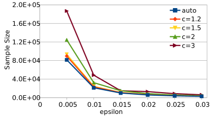
Figure 1: Final sample size for different sample schedules on P2p-Gnutella

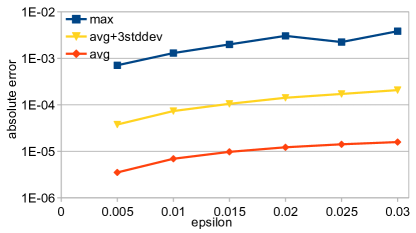
Figure 2: Absolute error evaluation – Soc-Epinions1

6.3 Accuracy

We evaluate the accuracy of ABRA-s by measuring the absolute error $|\widetilde{\mathsf{b}}(v)-\mathsf{b}(v)|$. The theoretical analysis guarantees that this quantity should be at most $\varepsilon$ for all nodes, with probability at least $1-\delta$. A first important result is that in all the thousands of runs of ABRA-s, the maximum error was always smaller than $\varepsilon$ (not just with probability $>1-\delta$). We report statistics about the absolute error in the three rightmost columns of Table 2 and in Fig. 2 (figures for the other graphs are in Appendix C. The minimum error (not reported) was always 0. The maximum error is an order of magnitude smaller than $\varepsilon$, and the average error is around three orders of magnitude smaller than $\varepsilon$, with a very small standard deviation. As expected, the error grows as $\varepsilon^{-2}$. In Fig. 2 we show the behavior of the maximum, average, and average plus three standard deviations (approximately corresponding to the 95% percentile) for Soc-Epinions1 (the vertical axis has a logarithmic scale), to appreciate how most of the errors are almost two orders of magnitude smaller than $\varepsilon$.

All these results show that ABRA-s is very accurate, more than what is guaranteed by the theoretical analysis. This can be explained by the fact that the bounds to the sampling size, the stopping condition, and the sample schedule are conservative, in the sense that we may be sampling more than necessary to obtain an $(\varepsilon,\delta)$-approximation. Tightening any of these components would result in a less conservative algorithm that still offers the same approximation quality guarantees, and is an interesting research direction.

6.4 Dynamic BC Approximation

We did not evaluate ABRA-d experimental, but, given its design, one can expect that, when compared to previous contributions offering the same quality guarantees [8, 21], it would exhibit similar or even larger speedups and reduction in the sample size than what ABRA-s had w.r.t. RK. Indeed, the algorithm by Bergamini and Meyerhenke [7] uses RK as a building block and it needs to constantly keep track of (an upper bound to) the vertex diameter of the graph, a very expensive operation. On the other hand, the analysis of the sample size by Hayashi et al. [21] uses very loose simultaneous deviation bounds (the union bound). As already shown by Riondato and Kornaropoulos [31], the resulting sample size is extremely large and they already showed how RK can use a smaller sample size. Since we built over the work by Hayashi et al. [21] and ABRA-s improves over RK, we can reasonably expect it to have much better performances than the algorithm by Hayashi et al. [21]

7 Conclusions

We presented ABRA, a family of sampling-based algorithms for computing and maintaining high-quality approximations of (variants of) the bc of all vertices in a graph. Our algorithms can handle static and dynamic graphs with edge updates (both deletions and insertions). We discussed a number of variants of our basic algorithms, including finding the top-$k$ nodes with higher bc, using improved estimators, and special cases when there is a single SP. ABRA greatly improves, theoretically and experimentally, the current state of the art. The analysis relies on Rademacher averages and on pseudodimension. To our knowledge this is the first application of these concepts to graph mining.

In the future we plan to investigate stronger bounds to the Rademacher averages, give stricter bounds to the sample complexity of bc by studying the pseudodimension of the class of functions associated to it, and extend our study to other network measures.

Acknowledgements. The authors are thankful to Elisabetta Bergamini and Christian Staudt for their help with the NetworKit code.

This work was supported in part by NSF grant IIS-1247581 and NIH grant R01-CA180776.

Appendix A Relative-error Top-k Approximation

In this section we prove the correctness of the algorithm ABRA-k (Thm. 6). The pseudocode can be found in Algorithm 2.

of Thm. 6.

With probability at least $1-\delta^{\prime}$, the set $\tilde{B}^{\prime}$ computed during the first phase (execution of ABRA-s) has the properties …. With probability at least $1-\delta^{\prime\prime}$, the set $\tilde{B}^{\prime\prime}$ computed during the second phase (execution of ABRA-s) has the properties from Thm. 5. Suppose both these events occur, which happens with probability at least $1-\delta$. Consider the value $\ell^{\prime}$. It is straightforward to check that $\ell^{\prime}$ is a lower bound to $b_{k}$: indeed there must be at least $k$ nodes with exact bc at least $\ell^{\prime}$. For the same reasons, and considering the fact that we run ABRA-r with parameters $\varepsilon$, $\delta^{\prime\prime}$, and $\lambda=\ell^{\prime}$, we have that $\ell^{\prime\prime}\leq b_{k}$. From this and the definition of $\widetilde{\mathsf{TOP}}(k,G)$, it follows that the elements of $\widetilde{\mathsf{TOP}}(k,G)$ are such that their exact may be greater than $\ell^{\prime\prime}$, and therefore of $b_{k}$. This means that $\mathsf{TOP}(k,G)\subseteq\widetilde{TOP}(k,G)$. The other properties of $\widetilde{TOP}(k,G)$ follow from the properties of the output of ABRA-r. ∎

input : Graph $G=(V,E)$, accuracy parameter $\varepsilon\in(0,1)$, confidence parameter $\delta\in(0,1)$, value $k\geq 1$

output : Set $\widetilde{B}$ of approximations of the bc of the top-$k$ vertices in $V$ with highest bc

1 $\delta^{\prime},\delta^{\prime\prime}\leftarrow$ reals such that $(1-\delta_{1})(1-\delta_{2})\geq 1-\delta$

2 $\widetilde{B}^{\prime}\leftarrow$ output of ABRA-s run with input $G,\varepsilon,\delta^{\prime}$

3 $\ell^{\prime}\leftarrow$ $k$-th highest value in $\widetilde{B}^{\prime}$

4 $\tilde{b}^{\prime}=\ell^{\prime}-\varepsilon$

5 $\widetilde{B}\leftarrow$ output of a variant of ABRA-s using the definition of $\Delta_{i}$ from (14), and input $G,\varepsilon,\delta^{\prime\prime},\tilde{b}^{\prime}$

6 return $\widetilde{B}$

Algorithm 2 ABRA-k: relative-error approximation of top-$k$ bc nodes on static graph

Appendix B Special Cases

In this section we expand on our discussion from Sect. 4.3. Since our results rely on pseudodimension [30], we start with a presentation of the fundamental definitions and results about pseudodimension.

B.1 Pseudodimension

Before introducing the pseudodimension, we must recall some notions and results about the Vapnik-Chervonenkis (VC) dimension. We refer the reader to the books by Shalev-Shwartz and Ben-David [34] and by Anthony and Bartlett [3] for an in-depth exposition of VC-dimension and pseudodimension.

Let $D$ be a domain and let $\mathcal{R}$ be a collection of subsets of $D$ ($\mathcal{R}\subseteq 2^{D}$). We call $\mathcal{R}$ a rangeset on $D$. Given $A\subseteq D$, the projection of $\mathcal{R}$ on $A$ is $P_{\mathcal{R}}(A)=\{R\cap A\leavevmode\nobreak\ :\leavevmode\nobreak\ R\in\mathcal{R}\}$. When $P_{\mathcal{R}}(A)=2^{A}$, we say that $A$ is shattered by $\mathcal{R}$. Given $B\subseteq D$, the empirical VC-dimension of $\mathcal{R}$, denoted as $\mathsf{E}\mathsf{VC}(\mathcal{R},B)$ is the size of the largest subset of $B$ that can be shattered. The VC-dimension of $\mathcal{R}$, denoted as $\mathsf{VC}(\mathcal{R})$ is defined as $\mathsf{VC}(\mathcal{R})=\mathsf{E}\mathsf{VC}(\mathcal{R},D)$.

Let $\mathcal{F}$ be a class of functions from some domain $D$ to $[0,1]$. Consider, for each $f\in\mathcal{F}$, the subset $R_{f}$ of $D\times[0,1]$ defined as

$$R_{f}=\{(x,t)\leavevmode\nobreak\ :\leavevmode\nobreak\ t\leq f(x)\}\enspace.$$

We define a rangeset $\mathcal{F}^{+}$ on $D\times[0,1]$ as $\mathcal{F}^{+}=\{R_{f},f\in\mathcal{F}\}$. The empirical pseudodimension [30] of $\mathcal{F}$ on a subset $B\subseteq D$, denoted as $\mathsf{E}\mathsf{PD}(\mathcal{F},B)$, is the empirical VC-dimension of $\mathcal{F}^{+}$: $\mathsf{E}\mathsf{PD}(\mathcal{F},B)=\mathsf{E}\mathsf{VC}(\mathcal{F}^{+},B)$. The pseudodimension of $\mathcal{F}$, denoted as $\mathsf{PD}(\mathcal{F})$ is the VC-dimension of $\mathcal{F}^{+}$, $\mathsf{PD}(\mathcal{F})=\mathsf{VC}(\mathcal{F}^{+})$ [3, Sect. 11.2]. Having an upper bound to the pseudodimension of $\mathcal{F}$ allows to bound the supremum of the deviations from (2), as stated in the following result.

Theorem 9 ([26], see also [19]).

Let $D$ be a domain and $\mathcal{F}$ be a family of functions from $D$ to $[0,1]$. Let $\mathsf{PD}(\mathcal{F})\leq d$. Given $\varepsilon,\delta\in(0,1)$, let $\mathcal{S}$ be a collection of elements sampled independently and uniformly at random from $D$, with size

$$|\mathcal{S}|=\frac{c}{\varepsilon^{2}}\left(d+\log\frac{1}{\delta}\right)\enspace.$$ (15)

Then

$$\Pr\left(\exists f\in\mathcal{F}\mbox{ s.t. }\left|\mathsf{m}_{D}(f)-\mathsf{m}_{\mathcal{S}}(f)\right|>\varepsilon\right)<\delta\enspace.$$

The constant $c$ is universal and it is less than 0.5 [27].

The following two technical lemmas are, to the best of our knowledge, new. We use them later to bound the pseudodimension of a family of functions related to betweenness centrality.

Lemma 1.

Let $B\subseteq D\times[0,1]$ be a set that is shattered by $\mathcal{F}^{+}$. Then $B$ can contain at most one element $(d,x)\in D\times[0,1]$ for each $d\in D$.

Proof.

Let $d\in D$ and consider any two distinct values $x_{1},x_{2}\in[0,1]$. Let, w.l.o.g., $x_{1}<x_{2}$ and let $B=\{(\tau,x_{1}),(\tau,x_{2})\}$. From the definitions of the ranges, there is no $R\in\mathcal{F}^{+}$ such that $R\cap B=\{(d,x_{1})\}$, therefore $B$ can not be shattered, and so neither can any of its supersets, hence the thesis. ∎

Lemma 2.

Let $B\subseteq D\times[0,1]$ be a set that is shattered by $\mathcal{F}^{+}$. Then $B$ does not contain any element in the form $(d,0)$, for any $d\in D$.

Proof.

For any $d\in D$, $(d,0)$ is contained in every $R\in\mathcal{F}^{+}$, hence given a set $B=\{(d,0)\}$ it is impossible to find a range $R_{\emptyset}$ such that $B\cap R_{\emptyset}=\emptyset$, therefore $B$ can not be shattered, nor can any of its supersets, hence the thesis. ∎

B.2 Pseudodimension for BC

We now move to proving the results in Sect. 4.3.

Let $G=(V,E)$ be a graph, and consider the family

$$\mathcal{F}=\{f_{w},w\in V\}$$

where $f_{w}$ goes from $\mathcal{D}=\{(u,v)\in V\times V,u\neq v\}$ to $[0,1]$ and is defined in (9). The rangeset $\mathcal{F}^{+}$ contains one range $R_{w}$ for each node $w\in V$. The set $R_{w}\subseteq\mathcal{D}\times[0,1]$ contains pairs in the form $((u,v),x)$, with $(u,v)\in\mathcal{D}$ and $x\in[0,1]$. The pairs $((u,v),x)\in R_{w}$ with $x>0$ are all and only the pairs with this form such that

1. $w$ is on a SP from $u$ to $v$; and

2. $x\leq\sigma_{uv}(w)/\sigma_{uv}$.

We now prove a result showing that some subsets of $\mathcal{D}\times[0,1]$ can not be shattered by $\mathcal{F}^{+}$, on any graph $G$. Thm. 7 follows immediately from this result, and Corollary 1 then follows from Thms. 7 and 9.

Lemma 3.

There exists no undirected graph $G=(V,E)$ such that it is possible to shatter a set

$$B=\{((u_{i},v_{i}),x_{i}),1\leq i\leq 4\}\subseteq\mathcal{D}\times[0,1]$$

if there are at least three distinct values $j^{\prime},j^{\prime\prime},j^{\prime\prime\prime}\in[1,4]$ for which

$$\sigma_{u_{j^{\prime}}v_{j^{\prime}}}=\sigma_{u_{j^{\prime\prime}}v_{j^{\prime\prime}}}=\sigma_{u_{j^{\prime\prime\prime}}v_{j^{\prime\prime\prime}}}=1\enspace.$$

Proof.

First of all, according to Lemmas 1 and 2, for $B$ to be shattered it must be

$$(u_{i},v_{i})\neq(u_{j},v_{j})\mbox{ for }i\neq j$$

and $x_{i}\in(0,1]$, $1\leq i\leq 4$.

Riondato and Kornaropoulos [31, Lemma 2] showed that there exists no undirected graph $G=(V,E)$ such that it is possible to shatter $B$ if

$$\sigma_{u_{1}v_{1}}=\sigma_{u_{2}v_{2}}=\sigma_{u_{3}v_{3}}=\sigma_{u_{4}v_{4}}=1\enspace.$$

Hence, what we need to show to prove the thesis is that it is impossible to build an undirected graph $G=(V,E)$ such that $\mathcal{F}^{+}$ can shatter $B$ when the elements of $B$ are such that

$$\sigma_{u_{1}v_{1}}=\sigma_{u_{2}v_{2}}=\sigma_{u_{3}v_{3}}=1$$

and $\sigma_{u_{4}v_{4}}=2$.

Assume now that such a graph $G$ exists and therefore $B$ is shattered by $\mathcal{F}^{+}$.

For $1\leq i\leq 3$, let $p_{i}$ be the unique SP from $u_{i}$ to $v_{i}$, and let $p_{4}^{\prime}$ and $p_{4}^{\prime\prime}$ be the two SPs from $u_{4}$ to $v_{4}$.

First of all, notice that if any two of $p_{1}$, $p_{2}$, $p_{3}$ meet at a node $a$ and separate at a node $b$, then they can not meet again at any node before $a$ or after $b$, as otherwise there would be multiple SPs between their extreme nodes, contradicting the hypothesis. Let this fact be denoted as $\mathsf{F}_{1}$.

Since $B$ is shattered, its subset

$$A=\{((u_{i},v_{i}),x_{i}1\leq i\leq 3\}\subset B$$

is also shattered, and in particular it can be shattered by a collection of ranges that is a subset of a collection of ranges that shatters $B$. We now show some facts about the properties of this shattering which we will use later in the proof.

Define

$$i^{+}=\left\{\begin{array}[]{ll}i+1&\mbox{if }i=1,2\\ 1&\mbox{if }i=3\end{array}\right.$$

and

$$i^{-}=\left\{\begin{array}[]{ll}3&\mbox{if }i=1\\ i-1&\mbox{if }i=2,3\end{array}\right.\enspace.$$

Let $v_{A}$ be a node such that $R_{v_{A}}\cap A=A$. For any $i$, $1\leq i\leq 3$, let $v_{i,i^{+}}$ be the node such that

$$R_{v_{i,i^{+}}}\cap A=\{(u_{i},v_{i}),(u_{i^{+}},v_{i^{+}}\}\enspace.$$

Analogously, let $v_{i,i^{-}}$ be the node such that

$$R_{v_{i,i^{-}}}\cap A=\{(u_{i},v_{i}),(u_{i^{-}},v_{i^{-}}\}\enspace.$$

We want to show that $v_{A}$ is on the SP connecting $v_{i,i^{+}}$ to $v_{i,i^{-}}$. Assume it was not. Then we would have that either $v_{i,i^{+}}$ is between $v_{A}$ and $v_{i,i^{-}}$ or $v_{i,i^{-}}$ is between $v_{A}$ and $v_{i,i^{+}}$. Assume it was the former (the latter follows by symmetry). Then

1. there must be a SP $p^{\prime}$ from $u_{i^{-}}$ to $v_{i^{+}}$ that goes through $v_{i,i^{-}}$;

2. there must be a SP $p^{\prime\prime}$ from $u_{i^{-}}$ to $v_{i^{+}}$ that goes through $v_{A}$;

3. there is no SP from $u_{i^{-}}$ to $v_{i^{+}}$ that goes through $v_{i,i^{+}}$.

Since there is only one SP from $u_{i^{-}}$ to $v_{i^{-}}$, it must be that $p^{\prime}=p^{\prime\prime}$. But then $p^{\prime}$ is a SP that goes through $v_{i,i-}$ and through $v_{A}$ but not through $v_{i,i^{+}}$, and $p_{i}$ is a SP that goes through $v_{i,i^{-}}$, through $v_{i,i^{+}}$ and through $v_{A}$ (either in this order or in the opposite). This means that there are at least two SPs between $v_{i,i^{-}}$ and $v_{A}$, and therefore there would be two SPs between $u_{i}$ and $v_{i}$, contradicting the hypothesis that there is only one SP between these nodes. Hence it must be that $v_{A}$ is between $v_{i,i^{-}}$ and $v_{i,i^{+}}$. This is true for all $i$, $1\leq i\leq 3$. Denote this fact as $\mathsf{F}_{2}$.

Consider now the nodes $v_{i,4}$ and $v_{j,4}$. We now show that they can not belong to the same SP from $u_{4}$ and $v_{4}$.

• Assume that $v_{i,4}$ and $v_{j,4}$ are on the same SP $p$ from $u_{4}$ to $v_{4}$ and assume that $v_{i,j,4}$ is also on $p$. Consider the possible orderings of $v_{i,4}$, $v_{j,4}$ and $v_{i,j,4}$ along $p$.

  • If the ordering is $v_{i,4}$, then $v_{j,4}$, then $v_{i,j,4}$ or $v_{j,4}$, then $v_{j,4}$, then $v_{i,j,4}$, or the reverses of these orderings (for a total of four orderings), then it is easy to see that fact $\mathsf{F}_{1}$ would be contradicted, as there are two different SPs from the first of these nodes to the last, one that goes through the middle one, and one that does not, but then there would be two SPs between the pair of nodes $(u_{k},v_{k})$ where $k$ is the index in $\{1,2,3\}$ different than $4$ that is in common between the first and the last nodes in this ordering, and this would contradict the hypothesis, so these orderings are not possible.

  • Assume instead the ordering is such that $v_{i,j,4}$ is between $v_{i,4}$ and $v_{j,4}$ (two such ordering exist). Consider the paths $p_{i}$ and $p_{j}$. They must meet at some node $v_{f_{i,j}}$ and separate at some node $v_{l_{i,j}}$. From the ordering, and fact $\mathsf{F}_{1}$, $v_{i,j,4}$ must be between these two nodes. From fact $\mathsf{F}_{2}$ we have that also $v_{A}$ must be between these two nodes. Moreover, neither $v_{i,4}$ nor $v_{j,4}$ can be between these two nodes. But then consider the SP $p$. This path must go together with $p_{i}$ (resp. $p_{j}$) from at least $p_{i,4}$ (resp. $p_{j,4}$) to the farthest between $v_{f_{i,j}}$ and $v_{l_{i,j}}$ from $p_{i,4}$ (resp. $p_{j,4}$). Then in particular $p$ goes through all nodes between $v_{f_{i,j}}$ and $v_{l_{i,j}}$ that $p_{i}$ and $p_{j}$ go through. But since $v_{A}$ is among these nodes,and $v_{A}$ can not belong to $p$, this is impossible, so these orderings of the nodes $v_{i,4}$, $v_{j,4}$, and $v_{i,j,4}$ are not possible.

  Hence we showed that $v_{i,4}$, $v_{j,4}$, and $v_{i,j,4}$ can not be on the same SP from $u_{4}$ to $v_{4}$.

• Assume now that $v_{i,4}$ and $v_{j,4}$ are on the same SP from $u_{4}$ to $v_{4}$ but $v_{i,j,4}$ is on the other SP from $u_{4}$ to $v_{4}$ (by hypothesis there are only two SPs from $u_{4}$ to $v_{4}$). Since what we prove in the previous point must be true for all choices of $i$ and $j$, we have that all nodes $v_{h,4}$, $1\leq h\leq 3$, must be on the same SP from $u_{4}$ to $v_{4}$, and all nodes in the form $v_{i,j,4}$, $1\leq i<j\leq 3$ must be on the other SP from $u_{4}$ to $v_{4}$. Consider now these three nodes, $v_{1,2,4}$, $v_{1,3,4}$, and $v_{2,3,4}$ and consider their ordering along the SP from $u_{4}$ to $v_{4}$ that they lay on. No matter what the ordering is, there is an index $h\in\{1,2,3\}$ such that the shortest path $p_{h}$ must go through the extreme two nodes in the ordering but not through the middle one. But this would contradict fact $\mathsf{F}_{1}$, so it is impossible that we have $v_{i,4}$ and $v_{j,4}$ on the same SP from $u_{4}$ to $v_{4}$ but $v_{i,j,4}$ is on the other SP, for any choice of $i$ and $j$.

We showed that the nodes $v_{i,4}$ and $v_{j,4}$ can not be on the same SP from $u_{4}$ to $v_{4}$. But this is true for any choice of the unordered pair $(i,j)$ and there are three such choices, but only two SPs from $u_{4}$ to $v_{4}$, so it is impossible to accommodate all the constraints requiring $v_{i,4}$ and $v_{j,4}$ to be on different SPs from $u_{4}$ to $v_{4}$. Hence we reach a contradiction and $B$ can not be shattered. ∎

The following lemma shows that the bound in Lemma 3 is tight.

Lemma 4.

There is an undirected graph $G=(V,E)$ such that there is a set $\{(u_{i},v_{i}),u_{i},v_{i}\in V,u_{i}\neq v_{i},1\leq i\leq 4\}$ with $|\mathsf{S}_{u_{1},v_{1}}|=|\mathsf{S}_{u_{2},v_{2}}|=2$ and $|\mathsf{S}_{u_{3},v_{3}}|=|\mathsf{S}_{u_{4},v_{4}}|=1$ that is shattered.

Figure 3: Graph for Lemma 4

Proof.

Consider the undirected graph $G=(V,E)$ in Fig. 3. There is a single SP from $0$ to $16$:

$$0,1,2,22,21,35,20,19,18,15,16\enspace.$$

There is a single SP from $23$ to $17$:

$$23,24,25,26,27,36,20,19,18,15,17\enspace.$$

There are exactly two SPs from $5$ to $33$:

$$5,4,3,2,22,26,25,28,39,33\mbox{ and}$$

$$5,6,7,18,18,29,30,32,40,33\enspace.$$

There are exactly two SPs from $11$ to $34$:

$$11,10,9,8,21,22,26,27,37,34\mbox{ and}$$

$$11,12,13,14,15,18,29,31,38,34\enspace.$$

Let $a=((0,16),1)$, $b=((23,17),1)$, $c=((5,33),1/2)$, and $d=((11,34),1/2)$. We can shatter the set $Q=\{a,b,c,d\}$, as shown in Table 3. ∎

$P\subseteq Q$	Vertex $v$ such that $P=Q\cap R_{v}$
$\emptyset$	0
$\{a\}$	1
$\{b\}$	24
$\{c\}$	40
$\{d\}$	38
$\{a,b\}$	20
$\{a,c\}$	2
$\{a,d\}$	21
$\{b,c\}$	25
$\{b,d\}$	27
$\{c,d\}$	29
$\{a,b,c\}$	19
$\{a,b,d\}$	15
$\{a,c,d\}$	22
$\{b,c,d\}$	26
$\{a,b,c,d\}$	18

Table 3: How to shatter $Q=\{a,b,c,d\}$ from Lemma 4.

We pose the following conjecture, which would allow us to generalize Lemma 3, and develop an additional stopping rule for ABRA-s based on the empirical pseudodimension.

Conjecture 1.

Given $n>0$, there exists no undirected graph $G=(V,E)$ such that it is possible to shatter a set

$$B=\{((u_{i},v_{i}),x_{i}),1\leq i\leq n\}\subseteq\mathcal{D}\times[0,1]$$

if

$$\sum_{i=1}^{n}\sigma_{u_{i}v_{i}}|<\binom{n}{\lfloor n/2\rfloor}\enspace.$$

Appendix C Additional Experimental Results

In this section we show additional experimental results, mostly limited to additional figures like Figs. 1 and 2 but for other graphs. The figures we present here exhibits the exact same behavior as those in Sect. 6, and that is why we did not include include them in the main text. Figures corresponding to Fig. 1 are shown in Fig. 4 and those corresponding to Fig. 2 are shown in Fig. 5.

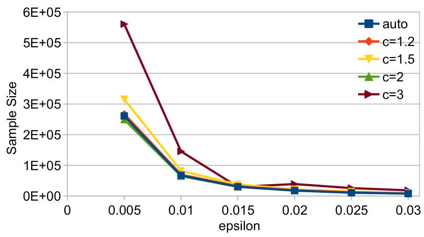
(a) Email-Enron

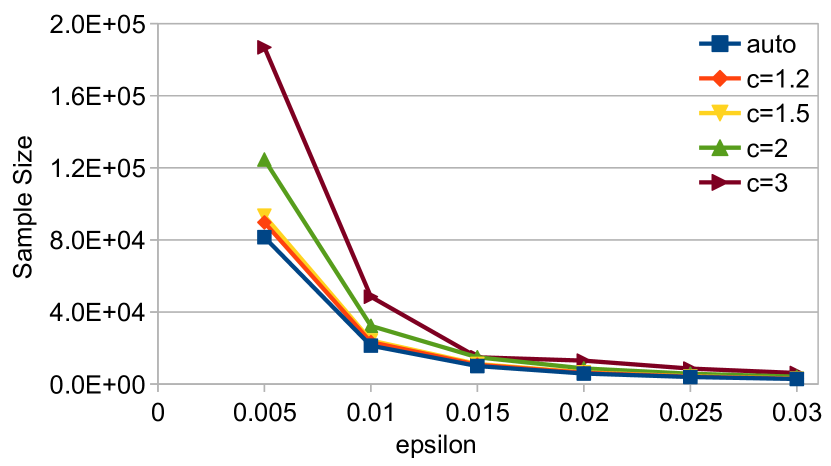
(b) Soc-Epinions1

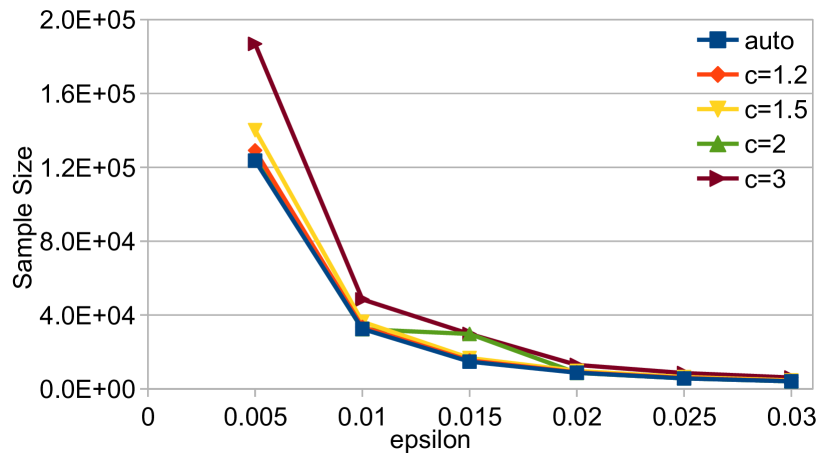
(c) Cit-HepPh

Figure 4: Final sample size for different sample schedules

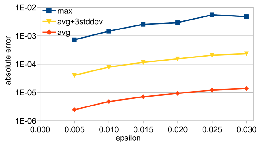
(a) Email-Enron

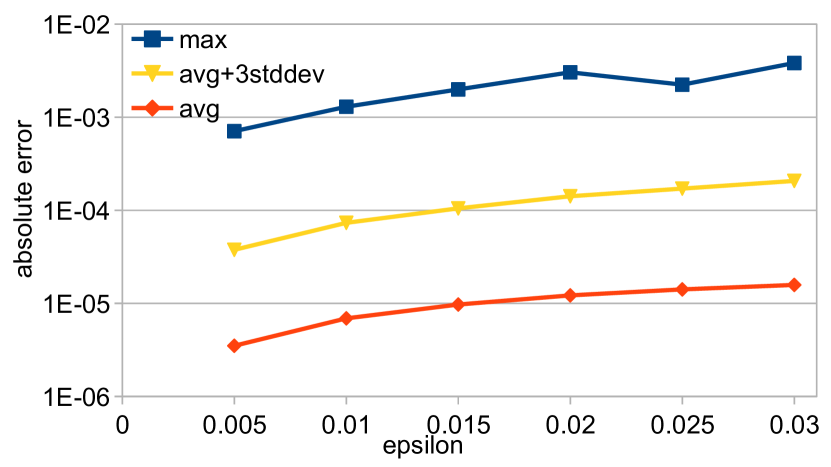
(b) Soc-Epinions1

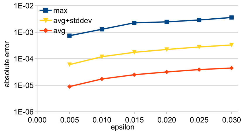
(c) Cit-HepPh

Figure 5: Absolute error evaluation

Appendix D Relative-error Rademacher Averages

In this note we show how to obtain relative $(p,\varepsilon)$-approximations as defined by Har-Peled and Sharir [19] (see Def. 3) using a relative-error variant of the Rademacher averages.

D.1 Definitions

Let $\mathcal{D}$ be some domain, and $\mathcal{F}$ be a family of functions from $\mathcal{D}$ to $[a,b]$, an interval of the non-negative reals. Assume that $\pi$ is a probability distribution on $\mathcal{D}$. For any $f\in\mathcal{F}$, let $\mathbb{E}_{\pi}[f]$ be the expected value of $f$ w.r.t. $\pi$. Let $A=\{a_{1},\dotsc,a_{n}\}$ be a collection of $n$ elements of $\mathcal{D}$. For any $f\in\mathcal{F}$, let

$$\tilde{f}(A)=\frac{1}{n}\sum_{i=1}^{n}f(a_{i})\enspace.$$

Definition 3 ([19]).

Given $p\in(0,1)$ and $\varepsilon\in(0,1)$, a relative $(p,\varepsilon)$-approximation for $\mathcal{F}$ is a collection $A$ of elements of $Z$ such that

$$\sup_{f\in\mathcal{F}}\frac{|\mathbb{E}_{\pi}[f]-\tilde{f}(A)|}{\max\{p,\mathbb{E}_{\pi}[f]\}}\leq\varepsilon\enspace.$$ (16)

Fixed-sample bound

Har-Peled and Sharir [19] showed that, when the functions of $\mathcal{F}$ only take values in $\{0,1\}$ and $\mathcal{F}$ has finite VC-dimension, then a sufficiently large collection $\mathcal{S}$ of $n$ elements of $\mathcal{D}$ sampled independently according to $\pi$ is a relative $(p,\varepsilon)$-approximation for $\mathcal{F}$ with probability at least $1-\delta$, for $\delta\in(0,1)$.

Theorem 10 (Thm. 2.11 [19]).

Let $\mathcal{F}$ be a family of functions from $\mathcal{D}$ to $\{0,1\}$, and let $d$ be the VC-dimension of $\mathcal{F}$. Given $p,\varepsilon,\delta\in(0,1)$, let

$$n=O\left(\frac{1}{\varepsilon^{2}p}\left(d\log\frac{1}{p}+\ln\frac{1}{\delta}\right)\right),$$ (17)

and let $\mathcal{S}$ be a collection of $n$ elements of $\mathcal{D}$ sampled independently according to $\pi$. Then,

$$\Pr\left(\sup_{f\in\mathcal{F}}\frac{|\mathbb{E}_{\pi}[f]-\tilde{f}(A)|}{\max\{p,\mathbb{E}_{\pi}[f]\}}>\varepsilon\right)<\delta,$$

or, in other words, $\mathcal{S}$ is a relative $(p,\varepsilon)$-approximation for $\mathcal{F}$ with probability at least $1-\delta$.

Related works

The bound in (17) is an extension of a result by Li et al. [26] obtained for families of real-valued functions taking values in $[0,1]$, and using the pseudodimension of the family instead of the VC-dimension. The original result by Li et al. [26] shows how large should $\mathcal{S}$ be in order for the quantity

$$\sup_{f\in\mathcal{F}}\frac{|\mathbb{E}_{\pi}[f]-\tilde{f}(\mathcal{S})|}{\mathbb{E}_{\pi}[f]+\tilde{f}(\mathcal{S})+p}$$ (18)

to be at most $\varepsilon$ with probability at least $1-\delta$. Some constant factors are lost in the adaptation of the measure from (18) to the one on the l.h.s. of (16). The quantity in (18) has been studied often in the literature of statistical learning theory, see for example [3, Sect. 5.5], [10, Sect. 5.1], and [20], while other works (e.g., [10, Sect. 5.1], [14], [4], and [6]) focused on the quantity

$$\sup_{f\in\mathcal{F}}\frac{|\mathbb{E}_{\pi}[f]-\tilde{f}(\mathcal{S})|}{\sqrt{\mathbb{E}_{\pi}[f]}}\enspace.$$

D.2 Obtaining a relative $(p,\varepsilon)$-approximation

In this note we study how to bound the quantity on the l.h.s. of (16) directly, without going through the quantity in (18). By following the same steps as [19, Thm. 2.9(ii)], we can extend our results to the quantity in (18). The advantage of tackling the problem directly is that we can derive sample-dependent bounds with explicit constants. Moreover, the use of (a variant of) Rademacher averages allows us to obtain stricter bounds to the sample size.

Let $\mathcal{S}=\{X_{1},\dotsc,X_{n}\}$ be a collection of $n$ elements from $\mathcal{D}$ sampled independently according to $\pi$. Let $\sigma_{1},\dotsc,\sigma_{n}$ be independent Rademacher random variables $\sigma_{1},\dotsc,\sigma_{n}$, independent from the samples. Consider now the random variable

$$\mathsf{r}\mathsf{R}(\mathcal{F},\mathcal{S},p)=\mathbb{E}_{\sigma}\left[\sup_{f\in\mathcal{F}}\frac{1}{n\max\{p,\mathbb{E}_{\pi}[f]\}}\sum_{i=1}^{n}\sigma_{i}f(X_{i})\right],$$

which we call the conditional $p$-relative Rademacher average of $\mathcal{F}$ on $\mathcal{S}$. We have the following result connecting this quantity to the $(p,\varepsilon)$ approximation condition.

Theorem 11.

Let $\mathcal{S}$ be a collection of $n$ elements of $\mathcal{D}$ sampled independently according to $\pi$. With probability at least $1-\delta$,

$$\sup_{f\in\mathcal{F}}\frac{|\mathbb{E}_{\pi}[f]-\tilde{f}(\mathcal{S})|}{\max\{p,\mathbb{E}_{\pi}[f]\}}\leq 2\mathsf{r}\mathsf{R}(\mathcal{S},\mathcal{F},p)+3\frac{|b-a|}{p}\sqrt{\frac{\ln(2/\delta)}{n}}\enspace.$$

The proof of Thm. 11 follows step by step the proof of Thm. 1 ([34, Thm. 26.4]), with the only important difference that we need to show that the quantities

$$\sup_{f\in\mathcal{F}}\frac{\mathbb{E}_{\pi}[f]-\tilde{f}(\mathcal{S})}{\max\{p,\mathbb{E}_{\pi}[f]\}}$$

and $\mathsf{r}\mathsf{R}(\mathcal{F},\mathcal{S},p)$, seen as functions of $\mathcal{S}=\{X_{1},\dotsc,X_{n}\}$, satisfy the bounded difference inequality.

Definition 4 (Bounded difference inequality).

Let $g:\mathcal{X}^{n}\rightarrow\mathbb{R}$ be a function of $n$ variables. The function $g$ is said to satisfy the bounded difference inequality iff for each $i$, $1\leq i\leq n$ there is a nonnegative constant $c_{i}$ such that:

$$\sup_{\begin{subarray}{c}x_{1},\dotsc,x_{n}\\ x_{i}^{\prime}\in\mathcal{X}\end{subarray}}|g(x_{1},\dotsc,x_{n})-g(x_{1},\dotsc,x_{i-1},x^{\prime}_{i},x_{i+1},\dotsc,x_{n})|\leq c_{i}\enspace.$$ (19)

We have the following results, showing that indeed the quantities above satisfy the bounded difference inequality.

Lemma 5.

The function

$$g(X_{1},\dotsc,X_{n})=\sup_{f\in\mathcal{F}}\frac{\mathbb{E}_{\pi}[f]-\tilde{f}(\mathcal{S})}{\max\{p,\mathbb{E}_{\pi}[f]\}}$$

satisfies the bounded difference inequality (19) with constants

$$c_{i}=\frac{|b-a|}{np}\enspace.$$

of Lemma 5.

Let $\mathcal{S}=\{X_{1},\dotsc,X_{n}\}$ and, for any $i$, $1\leq i\leq n$, let

$$\mathcal{S}^{\prime}_{i}=\{X_{1},\dotsc,X_{i-1},X^{\prime}_{i},X_{i+1},\dotsc,X_{n}\},$$

i.e., we replaced the random variable $X_{i}$ with another random variable $X^{\prime}_{i}$, sampled independently according to the same distribution. For any function $f\in\mathcal{F}$ let

$$\phi_{f}(\mathcal{S})=\frac{\mathbb{E}_{\pi}[f]-\tilde{f}(\mathcal{S})}{\max\{p,\mathbb{E}_{\pi}[f]\}}\enspace.$$

It is easy to see that

$$|\phi_{f}(\mathcal{S})-\phi_{f}(\mathcal{S}^{\prime}_{i})|\leq\frac{|b-a|}{np}$$ (20)

We have

$$|g(X_{1},\dotsc,X_{n})-g(X_{1},\dotsc,X_{i-1},X^{\prime}_{i},X_{i+1},\dotsc,X_{n})=$$

$$|g(\mathcal{S}^{\prime}_{i})-g(\mathcal{S})|=$$

$$\left|\sup_{f\in F}\phi_{f}(\mathcal{S}^{\prime}_{i})-\sup_{f\in F}\phi_{f}(\mathcal{S})\right|\enspace.$$ (21)

To simplify the notation, let now $\ell\in\mathcal{F}$ denote one of the functions for which the supremum is attained on $\mathcal{S}^{\prime}_{i}$, and let $h\in\mathcal{F}$ be on of the functions for which the supremum is attained on $\mathcal{S}$. Then we can rewrite (D.2) as

$$|\phi_{\ell}(\mathcal{S}^{\prime}_{i})-\phi_{h}(\mathcal{S})|\enspace.$$

Assume w.l.o.g. that

$$\phi_{h}(\mathcal{S})\leq\phi_{\ell}(\mathcal{S}^{\prime}_{i}),$$ (22)

(the other case follows by symmetry). We have

$$\phi_{\ell}(\mathcal{S})\leq\phi_{h}(\mathcal{S})$$ (23)

because $h$ attains the supremum over all possible $f\in F$ on $X_{1},\dotsc,X_{n}$. This and our assumption (22) imply that it must be

$$\phi_{\ell}(\mathcal{S})\leq\phi_{\ell}(\mathcal{S}^{\prime}_{i})\enspace.$$

From this and (20) we have

$$\phi_{\ell}(\mathcal{S}^{\prime}_{i})\leq\phi_{\ell}(\mathcal{S})+\frac{|b-a|}{np}\enspace.$$

Then from this and from (23) we have

$$\phi_{\ell}(\mathcal{S}^{\prime}_{i})-\phi_{h}(\mathcal{S})\leq\left(\phi_{\ell}(\mathcal{S})+\frac{|b-a|}{np}\right)-\phi_{\ell}(\mathcal{S})\leq\frac{|b-a|}{np}\enspace.$$

∎

Using the same steps as the above proof, we can prove the following result about the conditional $p$-relative Rademacher average.

Lemma 6.

The function

$$g(X_{1},\dotsc,X_{n})=\mathsf{r}\mathsf{R}(\{X_{1},\dotsc,X_{n}\},\mathcal{F},p)$$

satisfies the bounded difference inequality (19) with constants

$$c_{i}=\frac{|b-a|}{np}\enspace.$$

The following result is the analogous of Thm. 3 ([32, Thm. 3]) for the conditional $p$-relative Rademacher averages.

Theorem 12.

Let $\mathsf{w}_{\mathsf{r}}:\mathbb{R}^{+}\to\mathbb{R}^{+}$ be the function

$$\mathsf{w}_{\mathsf{r}}(s)=\frac{1}{s}\ln\displaystyle\sum_{\mathbf{v}\in\mathcal{V}_{\mathcal{S}}}\mathrm{exp}(s^{2}\|\mathbf{v}\|^{2}/p(2\ell^{2})),$$ (24)

where $\|\cdot\|$ denotes the Euclidean norm. Then

$$\mathsf{r}\mathsf{R}(\mathcal{F},\mathcal{S},p)\leq\min_{s\in\mathbb{R}^{+}}\mathsf{w}_{\mathsf{r}}(s)\enspace.$$ (25)

The proof follows the same steps as the one for [32, Thm. 3], with the additional initial observation that

$$\mathsf{r}\mathsf{R}(\mathcal{S},\mathcal{F},p)\leq\frac{1}{p}\mathsf{R}(\mathcal{S},\mathcal{F})\enspace.$$

References

- Anguita et al. [2014] D. Anguita, A. Ghio, L. Oneto, and S. Ridella. A deep connection between the Vapnik-Chervonenkis entropy and the Rademacher complexity. IEEE Transactions on Neural Networks and Learning Systems, 25(12):2202–2211, 2014.
- Anthonisse [1971] J. M. Anthonisse. The rush in a directed graph. Technical Report BN 9/71, Stichting Mathematisch Centrum, Amsterdam, Netherlands, 1971.
- Anthony and Bartlett [1999] M. Anthony and P. L. Bartlett. Neural Network Learning - Theoretical Foundations. Cambridge University Press, New York, NY, USA, 1999. ISBN 978-0-521-57353-5.
- Anthony and Shawe-Taylor [1993] M. Anthony and J. Shawe-Taylor. A result of Vapnik with applications. Discrete Applied Mathematics, 47(3):207–217, 1993.
- Bader et al. [2007] D. A. Bader, S. Kintali, K. Madduri, and M. Mihail. Approximating betweenness centrality. In A. Bonato and F. Chung, editors, Algorithms and Models for the Web-Graph, volume 4863 of Lecture Notes in Computer Science, pages 124–137. Springer Berlin Heidelberg, 2007. ISBN 978-3-540-77003-9. doi: 10.1007/978-3-540-77004-6_10.
- Bartlett and Lugosi [1999] P. L. Bartlett and G. Lugosi. An inequality for uniform deviations of sample averages from their means. Statistics & Probability Letters, 44(1):55–62, 1999.
- Bergamini and Meyerhenke [2015a] E. Bergamini and H. Meyerhenke. Fully-dynamic approximation of betweenness centrality. CoRR, abs/1504.0709 (to appear in ESA’15), Apr. 2015a.
- Bergamini and Meyerhenke [2015b] E. Bergamini and H. Meyerhenke. Approximating betweenness centrality in fully-dynamic networks. CoRR, abs/1510.07971, Oct 2015b. URL http://arxiv.org/abs/1510.07971.
- Bergamini et al. [2015] E. Bergamini, H. Meyerhenke, and C. L. Staudt. Approximating betweenness centrality in large evolving networks. In 17th Workshop on Algorithm Engineering and Experiments, ALENEX 2015, pages 133–146. SIAM, 2015.
- Boucheron et al. [2005] S. Boucheron, O. Bousquet, and G. Lugosi. Theory of classification : A survey of some recent advances. ESAIM: Probability and Statistics, 9:323–375, 2005.
- Boyd and Vandenberghe [2004] S. Boyd and L. Vandenberghe. Convex optimization. Cambridge university press, 2004.
- Brandes [2001] U. Brandes. A faster algorithm for betweenness centrality. J. Math. Sociol., 25(2):163–177, 2001. doi: 10.1080/0022250X.2001.9990249.
- Brandes and Pich [2007] U. Brandes and C. Pich. Centrality estimation in large networks. Int. J. Bifurcation and Chaos, 17(7):2303–2318, 2007. doi: 10.1142/S0218127407018403.
- Cortes et al. [2013] C. Cortes, S. Greenberg, and M. Mohri. Relative deviation learning bounds and generalization with unbounded loss functions. CoRR, abs/1310.5796, Oct 2013. URL http://arxiv.org/abs/1310.5796.
- Erdős et al. [2015] D. Erdős, V. Ishakian, A. Bestavros, and E. Terzi. A divide-and-conquer algorithm for betweenness centrality. In SIAM Data Mining Conf., 2015.
- Freeman [1977] L. C. Freeman. A set of measures of centrality based on betweenness. Sociometry, 40:35–41, 1977.
- Geisberger et al. [2008] R. Geisberger, P. Sanders, and D. Schultes. Better approximation of betweenness centrality. In J. I. Munro and D. Wagner, editors, Algorithm Eng. & Experiments (ALENEX’08), pages 90–100. SIAM, 2008.
- Green et al. [2012] O. Green, R. McColl, and D. Bader. A fast algorithm for streaming betweenness centrality. In Privacy, Security, Risk and Trust (PASSAT), 2012 International Conference on and 2012 International Confernece on Social Computing (SocialCom), pages 11–20, sep 2012. doi: 10.1109/SocialCom-PASSAT.2012.37.
- Har-Peled and Sharir [2011] S. Har-Peled and M. Sharir. Relative -approximations in geometry. Discrete & Computational Geometry, 45(3):462–496, 2011. ISSN 0179-5376. doi: 10.1007/s00454-010-9248-1.
- Haussler [1992] D. Haussler. Decision theoretic generalizations of the PAC model for neural net and other learning applications. Information and Computation, 100(1):78–150, 1992. ISSN 0890-5401.
- Hayashi et al. [2015] T. Hayashi, T. Akiba, and Y. Yoshida. Fully dynamic betweenness centrality maintenance on massive networks. Proceedings of the VLDB Endowment, 9(2), 2015.
- Kas et al. [2013] M. Kas, M. Wachs, K. M. Carley, and L. R. Carley. Incremental algorithm for updating betweenness centrality in dynamically growing networks. In Proceedings of the 2013 IEEE/ACM International Conference on Advances in Social Networks Analysis and Mining, ASONAM ’13, pages 33–40, New York, NY, USA, 2013. ACM. ISBN 978-1-4503-2240-9. doi: 10.1145/2492517.2492533. URL http://doi.acm.org/10.1145/2492517.2492533.
- Kourtellis et al. [2015] N. Kourtellis, G. D. F. Morales, and F. Bonchi. Scalable online betweenness centrality in evolving graphs. IEEE Trans. Knowl. Data Eng., 27(9):2494–2506, 2015. doi: 10.1109/TKDE.2015.2419666.
- Lee et al. [2012] M.-J. Lee, J. Lee, J. Y. Park, R. H. Choi, and C.-W. Chung. QUBE: A quick algorithm for updating betweenness centrality. In Proceedings of the 21st International Conference on World Wide Web, WWW ’12, pages 351–360, New York, NY, USA, 2012. ACM. ISBN 978-1-4503-1229-5. doi: 10.1145/2187836.2187884.
- Leskovec and Krevl [2014] J. Leskovec and A. Krevl. SNAP Datasets: Stanford large network dataset collection. http://snap.stanford.edu/data, June 2014.
- Li et al. [2001] Y. Li, P. M. Long, and A. Srinivasan. Improved bounds on the sample complexity of learning. J. Comp. Sys. Sci., 62(3):516–527, 2001. ISSN 0022-0000. doi: 10.1006/jcss.2000.1741.
- Löffler and Phillips [2009] M. Löffler and J. M. Phillips. Shape fitting on point sets with probability distributions. In A. Fiat and P. Sanders, editors, Algorithms - ESA 2009, volume 5757 of Lecture Notes in Computer Science, pages 313–324. Springer Berlin Heidelberg, 2009. doi: 10.1007/978-3-642-04128-0_29.
- Newman [2010] M. E. J. Newman. Networks – An Introduction. Oxford University Press, 2010.
- Oneto et al. [2013] L. Oneto, A. Ghio, D. Anguita, and S. Ridella. An improved analysis of the Rademacher data-dependent bound using its self bounding property. Neural Networks, 44:107–111, 2013.
- Pollard [1984] D. Pollard. Convergence of stochastic processes. Springer-Verlag, 1984.