Chaotic Advection at the Pore Scale: Mechanisms, Upscaling and Implications for Macroscopic Transport

Abstract

The macroscopic spreading and mixing of solute plumes in saturated porous media is ultimately controlled by processes operating at the pore scale. Whilst the conventional picture of pore-scale mechanical dispersion and molecular diffusion leading to persistent hydrodynamic dispersion is well accepted, this paradigm is inherently two-dimensional (2D) in nature and neglects important three-dimensional (3D) phenomena. We discuss how the kinematics of steady 3D flow at the pore-scale generate chaotic advection—involving exponential stretching and folding of fluid elements—the mechanisms by which it arises and implications of microscopic chaos for macroscopic dispersion and mixing. Prohibited in steady 2D flow due to topological constraints, these phenomena are ubiquitous due to the topological complexity inherent to all 3D porous media. Consequently 3D porous media flows generate profoundly different fluid deformation and mixing processes to those of 2D flow. The interplay of chaotic advection and broad transit time distributions can be incorporated into a continuous-time random walk (CTRW) framework to predict macroscopic solute mixing and spreading. We show how these results may be generalised to real porous architectures via a CTRW model of fluid deformation, leading to stochastic models of macroscopic dispersion and mixing which both honour the pore-scale kinematics and are directly conditioned on the pore-scale architecture.

1 Introduction

The migration and dispersion of solutes in groundwater systems is fundamental to chemical and biological reaction in the regolith. Solute transport in porous media is a well studied topic, and relevant dispersion, dilution and mixing process models have utility across a range of transport and reaction scenarios, including in contaminant remediation, in extraction of commodities (minerals, oil and gas), in surface water - groundwater interaction, and so on. In fact, more generally, fluid dispersion, dilution and mixing belong to a broad class of dissipative processes that mediate structure and instability in the geosciences, where thermal, hydrological, mechanical and chemical (THMC) phenomena are coupled over wide ranges of spatial and temporal scales [40, 39]. Evidence is growing that fluid dissipation processes manifesting at one scale can have profound influences on mechanical, thermal and chemical structures at larger scales. It is important to consider whether our understandings of solute transport in porous media are sufficient to underpin the rich set of dependent phenomena.

If we focus on the problem of solute transport in groundwater systems, the last forty years have seen growing sophistication of conceptual and theoretical tools, observations and predictions of spreading and reaction in solute plumes. Even so, there is still much to learn about how fluids and solutes migrate and mix in porous media, and how we may control or manipulate these transport processes for benefit. Despite recent advances in dynamical engineering of subsurface reactions at the macroscale [44, 31], significant questions about the scale dependence of plume dispersion, about solute mixing and about in situ biogeochemical reaction kinetics remain unresolved. It is our thesis that the resolution of these meso/macroscale questions lies at the pore scale, specifically in terms of the complex interplay between the pore space and fluid mechanics, and how this interplay upscales into observed plume characteristics. We contend that pore-scale dynamics engender characteristics of transport and mixing that persist through upscaling into the macroscopic domain and therefore play an important role in conditioning effective mixing and reaction phenomena in porous media.

Computer tomography (CT) has enabled significant advances in the understanding and prediction of pore scale fluid percolation, transport and reaction phenomena [5]. Using three-dimensional (3D) micro-CT scanning, it is possible to construct digital representations of pore spaces from physical samples, and then use numerical flow and transport solvers to track and predict fluid-borne phenomena in three dimensions. For example, Liu and Regenauer-Lieb [29] show how digital cores can be post-processed to characterise percolation thresholds and critical indices, which permits detailed upscaling of microscopic sample observations to effective macroscopic material properties. Kang et al. [15] use low-Reynolds number Navier-Stokes computations to show how the pore fluid velocity bursts observed in strongly heterogeneous systems are correlated with anomalous transport signatures at the micron scale in real rock samples. In a larger scale study, Alhashmi et al. [1] have imaged spherical bead assemblies and generated Stokes flow fields in the interstitial spaces. From these fields they were able to reconcile under-prediction of effective bimolecular reaction rates in terms of incomplete fluid mixing in the complex pore space. The digital imaging approach is also being used to progress detailed simulations of multiphase processes in complex pore geometries at the micron scale [37]. Together, these and other studies have shown that it is possible to link the microscale to the macroscale through a combination of high-resolution imaging, direct computation and upscaling techniques. However, dealing simultaneously with the complexities of topology, geometry and fluid reactions may obscure some of the component processes.

Stochastic models offer a means to deal with both the uncertainty and complexity of the both the pore-scale architecture and macroscopic heterogeneities, and to facilitate upscaling. The kernels of the stochastic models embody the physical properties of both the porous medium and the hosted processes. Whilst these models possess a great deal of flexibility with respect to capturing a wide range of (often anomalous) transport, mixing and reaction phenomena, it is important to develop strong linkages between the physical processes and the model kernels. The alternative approach is to create stochastic models with “black box” kernels derived from regression analysis, which provide limited physical insight into the process at hand, and hamper development of generalised models which may be readily applied to different media or chemical kinetics. This shortcoming often manifests as an upscaling failure - i.e. models which are conditioned upon observations at a particular length-scale fail at others, or cannot be readily translated to regimes with different Peclét or Damköhler numbers. Central to the development of so-called physically conditioned stochastic models is the need to derive models which capture the underlying fundamental dynamics and so recover the associated constraints and physical phenomena. As the kernels of these models are more tightly constrained they exhibit a reduced risk of spurious regression, are directly linked to the underlying physical processes, and so are more readily generalised across scales, media and processes.

In this paper we consider how the kinematics of steady 3D flow at the pore-scale influence macroscopic fluid mixing and chemical transport in saturated porous media, and how to develop upscaled models of dispersion and dilution which capture these processes. Our purpose here is to strengthen the conceptual linkages between pore-scale physics and macroscopic observations of solute transport and mixing in porous media. This paper describes concepts of pore scale topology and how they relate to transport of solutes in porous media. Dimensionality is a critical parameter. In contrast with common conceptual pictures of two dimensional branching of fluid streamlines used as a motivation for hydrodynamic dispersion, it is shown that proper consideration of truly 3D flow and transport at the pore scale admits wholly new transport mechanisms which are not readily apparent in conventional dispersion models. Specifically, 3D steady flow opens the door to the possibility of chaotic fluid trajectories [36], whereby fluid elements deform exponentially in time, leading to wholly different mixing and dispersion. Indeed, chaotic advection has been shown [25] to be inherent to steady 3D flow at the pore scale. Conversely, these dynamics are inadmissible in steady 2D flow, and so are neglected—or in fact not suspected to be needed—in conventional modelling frameworks.

Such chaotic (space-filling) transport dynamics are quite distinct from the conventional picture of hydrodynamic dispersion and can lead to persistent features that manifest in solute plumes at much greater spatial and temporal scales. The paper provides examples of persistent pore-scale chaotic phenomena, and then discusses some implications of pore-scale chaos for macroscopic transport. This topological approach to fluid physics at the pore scale is a relatively new area and opportunities abound for further development. The remainder of this paper is organised as follows; Section 2 discusses topology of the pore pace and implications for flow, Section 3 discusses the mechanisms which lead to chaotic advection at the pore scale, and in Section 4 fluid flow and transport are considered in a model open porous network. In Section 5 pore-scale mixing due to the interplay of chaotic advection and molecular diffusion is quantified, and the impact of these processes upon longitudinal dispersion is considered in Section 6. A discussion of approaches to extend the derived results to real porous media is presented in Section 7, and the paper concludes with some commentary on particularly promising research directions.

2 Fluid flow and deformation an the pore-scale

In general, as fluid mixing and dispersion involves the interplay of fluid deformation, advection and molecular diffusion, successful upscaling of these phenomena must capture the salient features of these processes at the micro-scale. The classical picture of flow and transport at the pore scale (e.g. Bear and Verruijt, 1987 [4]) typically involves the depiction of fluid streamline dynamics meandering through a 2D domain punctuated by an arbitrary array of inclusions, as depicted in Figure 1. This conceptual image illustrates the features which organise transport and dispersion but, if interpreted literally, the 2D nature of the fluid domain actually imposes severe constraints upon the admissible fluid dynamics, which in turn impact transport and mixing. Whilst conceptual, these topological constraints implicitly skew our understanding of the mechanisms which drive transport and mixing and neglect other important phenomena which may occur in 3D domains.

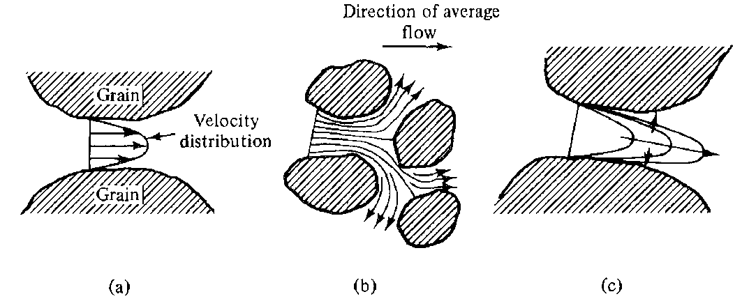
Figure 1: Conventional depiction of hydrodynamic dispersion mechanisms operating at the pore scale (the graphic is reproduced from [4]): (a) mechanical dispersion via Poisueille flow profiles at pore throats, (b) mechanical dispersion via flow separation at obstacles, (c) spreading due to molecular diffusion (Brownian motion).

Figure 2: Experimental image of hydrodynamic dispersion in 2D random porous media (mean flow is from left to right) illustrating splitting and recombination of fluid streamlines. Adapted from Bruyne et al [6].

For all steady 2D flows, an important topological constraint arises from the fact that the fluid acts as a continuum, and so streamlines cannot cross over each other, as reflected in Figure 1. As such, whilst the distance between neighbouring streamlines in 2D flows may fluctuate along a streamline, the separation distance cannot grow or shrink without bound due to conservation of mass. Although distance fluctuations can persist as streamlines pass either side of the stagnation points of grains and inclusions, eventually these streamlines must recombine, as shown in Figures 1,2. This topological constraint, which is formally imposed by the Poincaré-Bendixson theorem [43, 3], places significant restrictions on fluid deformation and hence transport of a diffusive scalar (solutes, heat etc) since no steady 2D flow can be chaotic - all such flows are regular with deformations which scale algebraically with time. Hence the only mechanism for persistent dispersion of solutes transverse to the mean flow direction is molecular diffusion. That is, transverse diffusion is the only physical means by which scalar quantities can spread transversely without bound in two dimensions to generate the observed lateral spreading of macroscale plumes. In contrast to the conventional picture of dispersion, the divergence of streamlines around inclusions (specifically, around stagnation points) is immaterial with respect to macroscopic transverse dispersion as eventually these streamlines must recombine downstream due to the topological constraint inherent to 2D steady flow.

However, this topological constraint does not apply to 3D steady flows, as the additional degree of freedom associated with the third spatial dimension removes the restriction that a fluid streamline is bounded by its neighbours, and so streamlines may wander much more freely throughout the pore space. As such, continua may deform in a more complex manner, and streamlines may now diverge or converge without bound even if the flow is incompressible. Hence, 3D transport is not simply a 3D extrusion of the dynamics shown in Figure 1, but rather 3D flows exhibit fundamentally different dynamics which introduce wholly new transport and mixing phenomena. It is these pore-scale dynamics that we shall explore and quantify in this study, and determine some of the related implications for macroscopic transport and dispersion.

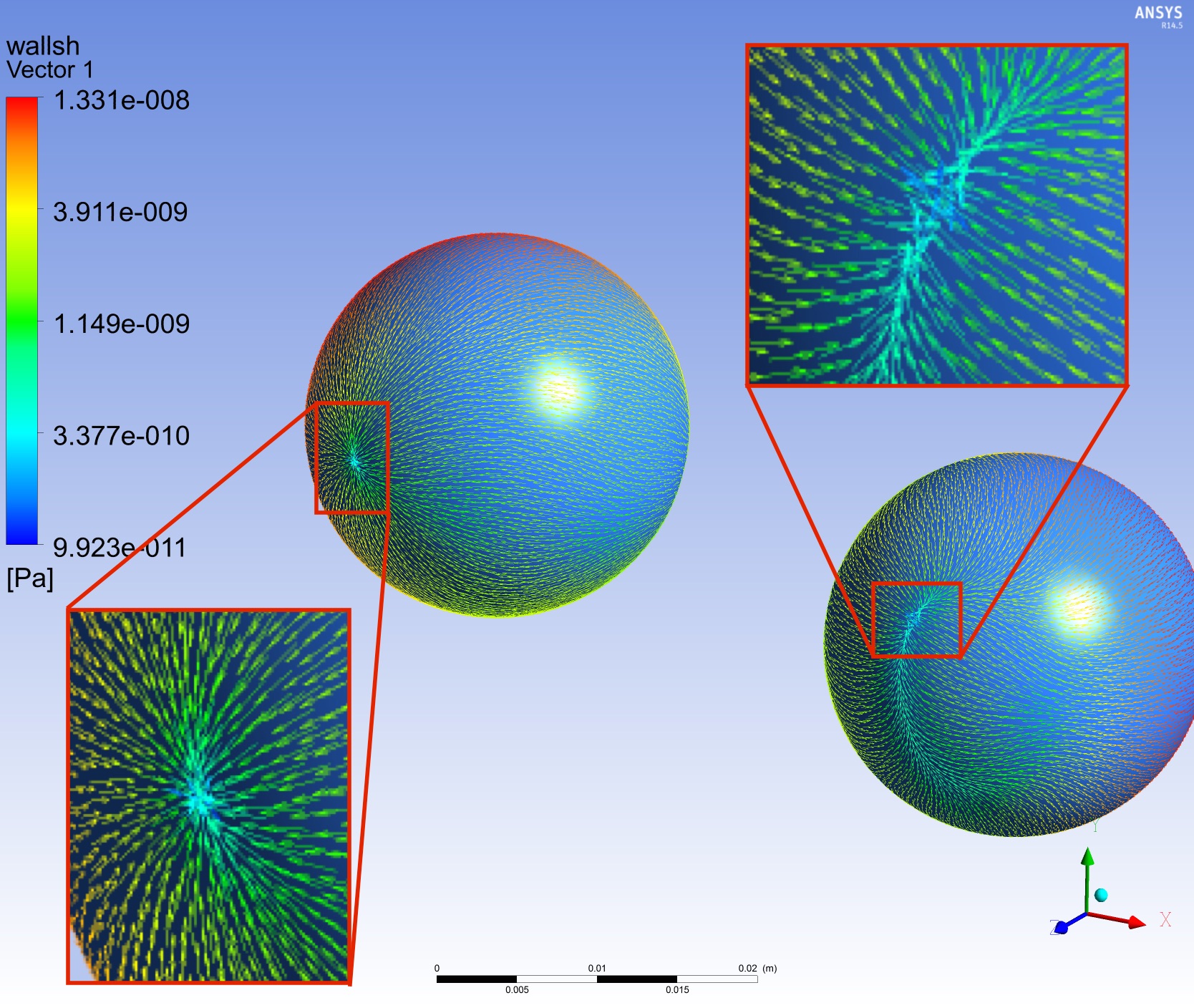
(a)

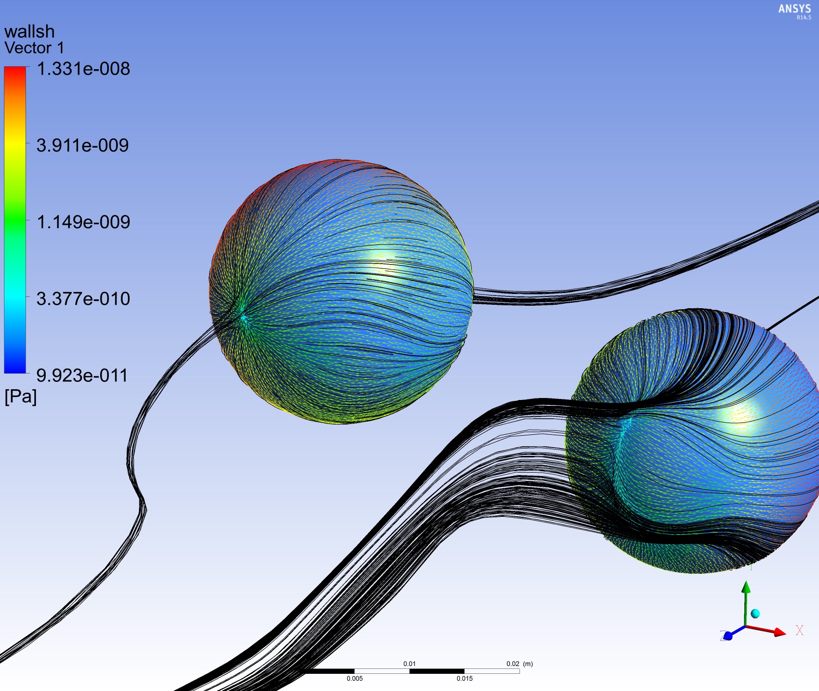
(b)

Figure 3: Computational simulations of 3D Stokes flow through a disordered array of spherical obstacles (only two spheres are shown). (a) Skin friction fields on sphere surfaces, showing minimum friction node point (left sphere) and locus (right sphere). (b) Panel (a) with streamlines drawn, showing a 1D unstable manifold downstream of the left sphere, and a 2D unstable manifold downstream of the right sphere. Image courtesy of Regis Turuban, University of Rennes.

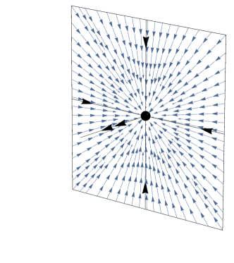
(a)	(b)

Figure 4: Schematic of the skin friction field (blue arrows) and 1D and 2D manifolds (black arrows, blue sheet) associated with an (a) node- and (b) saddle-type re-attachment point (black dot) shown in Figure 3.

To understand the mechanisms which govern dispersion and dilution at the pore scale, it is instructive to first consider the advection dynamics in the absence of molecular diffusion; these dynamics provides a template upon which diffusion, mixing and reaction play out. Whilst pore-scale fluid flow may appear to be a trivial process, in fact the Lagrangian advection dynamics can exhibit complex, chaotic behaviour, even in simple steady flows such as Stokes flow. Figure 3 shows the dynamics of a steady 3D Stokes flow over a random cluster of non-touching spheres (many spheres are present but only two are rendered), with particular attention paid to streamlines which pass very closely to the surface of the spheres shown and to the skin friction (surface stress) field over the surface of these spheres. The complexity of these streamlines is a direct consequence of the geometry of the spheres; these inclusions significantly perturb the flow in a manner which differs significantly from flow over an isolated sphere. Figure 3 illustrates that the downstream separatrix of the flow over a sphere can take the form of a point (analogous to 2D flow in Figure 1) or of a locus which generates a 2D sheet (or manifold) of streamlines, even if the upstream collection of streamlines is essentially one-dimensional (1D). Such stretching into 2D sheets is the fundamental building block of chaotic advection at the pore scale, and we shall see that in all disordered 3D geometries the repeated stretching into sheets is the norm rather than the exception: such stretching is ubiquitous to all random porous media.

The skin friction field itself causes transverse stretching of streamlines as they are ejected from near the surface of the sphere, and successive stretching events driven by these boundary dynamics lead to complex entanglements of streamlines as fluid elements encounter successive obstacles on the journey through a porous medium. In contrast to steady 2D flows, streamlines in 3D flows that are initially close are now free to diverge in such a manner that fluid elements between streamlines can become stretched exponentially with longitudinal distance without bound. As this unbounded exponential growth is contained within a finite domain, these 2D sheets are both stretched and folded into complex, highly striated (lamellar) distributions as they flow downstream. Hence, even a miniscule amount of molecular diffusion can lead to rapid mixing of these lamellar structures and exhibit significantly accelerated dilution, many orders of magnitude faster than that permitted by the 2D flows shown in Figure 1. In this way effective hydrodynamic dispersion can be far more prevalent and profound in genuinely 3D steady flows.

The key questions with respect to dispersion and dilution are, given the topological freedom associated with 3D flow, how prevalent is such streamline separation/diversion and what are the consequent impacts upon transport and mixing? How do these mechanisms manifest at the macroscale and what are the implications of pore-scale dimensionality for macroscale dispersion and dilution?

3 Chaos at the pore scale

As discussed in the previous Section, pore scale geometries and fluid processes are both complex and complicated. We contend, however, that by focusing on the essential topological features of these systems it is possible to understand and classify the dispersion and mixing dynamics without requiring precise descriptions of the pore network. We pursue a detailed understanding of the phenomena presented in Figure 3 and what dynamical consequences arise for such flows encountering a long succession of pore branches and merges. Whilst the phenomena in the figure are the result of highly idealized models, we shall demonstrate that the ingredients for such phenomena are inherent to all 3D random porous media, regardless of the specific details of the pore-scale architecture and so these mechanisms are completely ubiquitous.

To begin, the phenomena illustrated in Figure 3 are classical precursors of so-called chaotic advection in a steady 3D flow. Chaotic advection [2, 36] refers to a particular flow phenomenon which can arise in unsteady 2D or steady 3D flows whereby the advection equation

$$\frac{d\mathbf{x}}{dt}=\mathbf{v}(\mathbf{x},t),$$ (1)

describing the evolution of the position $\mathbf{x}$ of a fluid particle with time $t$ under the action of the flow field $\mathbf{v}(\mathbf{x},t)$ can give rise to chaotic dynamics in which fluid particles separate exponentially in time, losing memory of their initial neighborhoods and giving rise to complex fluid particle trajectories. The strength of the chaotic dynamics is characterized by the Lyapunov exponent $\lambda_{\infty}$ which measures the exponential growth rate of the length $\ell(t)$ of a fluid element of initial length $\ell_{0}$ with time as

$$\lambda_{\infty}=\lim_{t\rightarrow\infty}\frac{1}{t}\ln\frac{\ell(t)}{\ell_{0}}.$$ (2)

The Lyapunov exponent also acts as an indicator for chaotic dynamics as sub-exponential (i.e. algebraic) stretching results in $\lambda_{\infty}=0$. Due to conservation of mass, exponential longitudinal stretching of fluid elements must also be accompanied by equivalent exponential narrowing in at least one of the transverse directions, resulting in highly striated lamellar material distributions. To contain such elongated structures within a finite domain, both fluid stretching and folding is required, and these two motions are considered to be the hallmarks of chaotic dynamics in all continuous systems [36].

This stretching and folding process is known as chaotic advection, and represents an efficient means of fluid stirring akin to that of turbulent flow but available for acctuation in low Reynolds number, non-turbulent flows. The key difference between chaotic advection and turbulent mixing is that the advection equation (1) is an identity and so is kinematic rather than dynamic in origin, and so chaotic advection can arise under a broad range of dynamical regimes. Importantly, from (1), flows which have a simple structure in the Eulerian frame can generate complex Lagrangian dynamics and material distributions with arbitrarily small length scales. Since at sufficiently small length scales molecular diffusion—no matter how weak—plays a dominant role and leads to rapid dilution and homogenization of initially large-scale concentration distributions, chaos is the basis for accelerated mixing. This phenomenon is well documented [36, 46, 42, 32] and understood in low-Reynolds number flows such as Stokes and laminar flows, and forms the design basis of a wide range of micro-fluidic [41] and industrial [24] mixing devices, including static mixers [12] which operate on similar principles to the mixing dynamics in 3D porous media. Moreover, elucidation of these mixing mechanisms has provided significant insights into mixing and transport in nature, ranging from transport in geophysical flows [35] to population biology [16].

It is instructive to consider whether the mechanism of chaotic advection is relevant to transport in porous media; particularly with respect to dilution, mixing and macro-dispersion. For reasons that shall become apparent, we focus attention to pore-scale flow, under steady 3D Stokes flow, subject to no-slip boundary conditions. Whilst the concepts discussed apply to broader conditions than these (specifically any boundary condition and all steady flows of continua), these conditions serve well to elucidate the fundamental mechanisms.

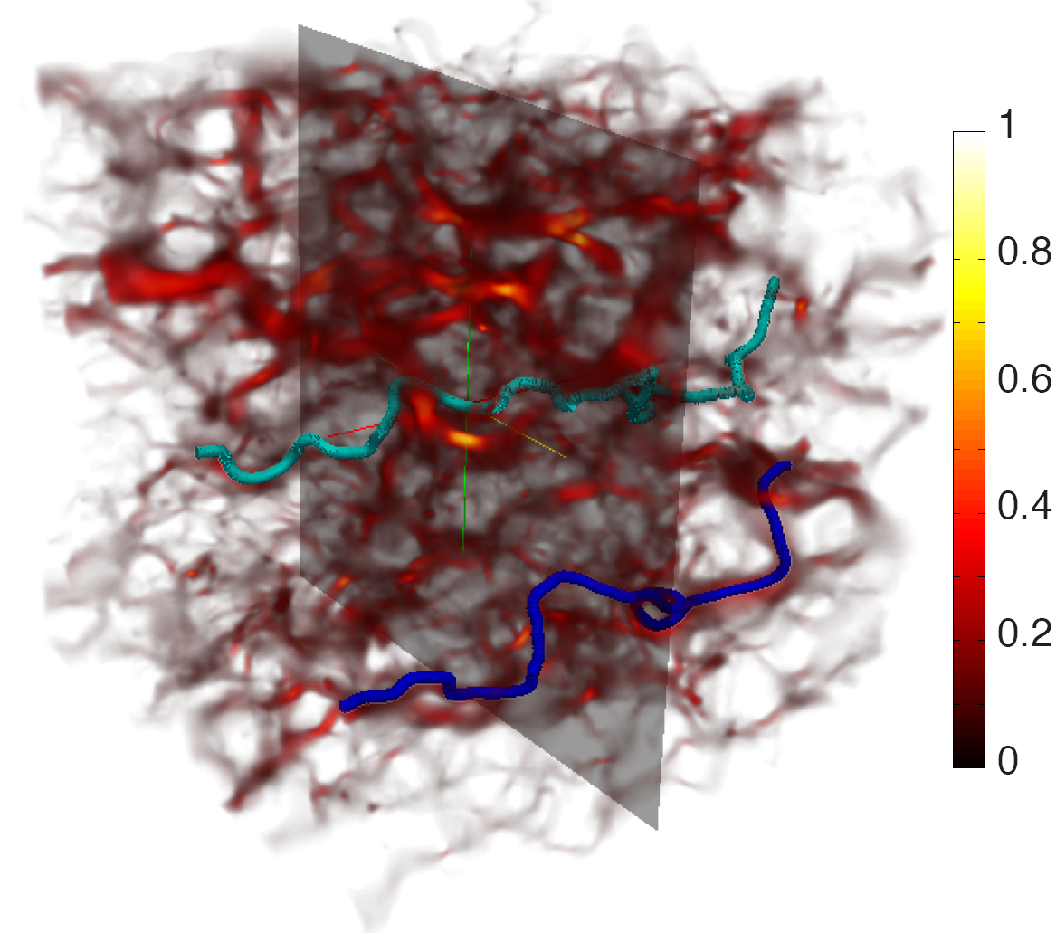
Figure 5: Digital reconstruction of the 3D flow field through a Berea sandstone block (1.6 mm cube). The normalized velocity magnitude is rendered according to the colour bar; yellow zones indicate high velocity bursts. Two flow paths (blue and cyan) show evidence of branch and merge behaviour. Adapted from Figure 1 of [15].

The key feature common to all porous media is topological complexity of the pore space, such that the pore-scale fluid domain is highly connected, and contains a large number of junctions and merges per unit volume, as illustrated by the blue and cyan flow paths in Figure 5). This defining property is common to all porous media, whether open porous networks, granular, fractured or synthetic media and has significant implications for flow and transport. Such complexity can be quantified via digital CT imaging of the pore space, allowing direct measurement of the number of pores $N$, redundant connections $C$ and enclosed cavities $H$ per unit volume [45]. These measures allow the connectivity at the pore scale to be directly quantified in terms of the topological genus $g$, which may be interpreted as the number of distinct “holes” an object possesses, such that a sphere is of genus zero, whilst a doughnut is of genus one, and a pretzel may be genus two, three or higher. The topological genus per unit volume of a porous medium is then directly related to the measures above [45] as

$$2(1-g)=N-C+H.$$ (3)

As all porous media are highly connected (topologically complex) at the pore scale, imaging studies typically find $N<C$ and $H$ small (except for foams and some vitreous rocks), and so $g$ is positive and large across a broad range of systems. This inherent topological complexity has significant implications for flow and transport at the pore-scale.

Remarkably, there exists a direct correspondence between pore-scale complexity (measured by $g$) and the number and type of stagnation points in the skin friction vector field (the shear stress field projected onto the pore boundary), such as those shown in Figure 3. A stagnation point $\mathbf{x}_{p}$ arises as a zero of the skin friction field $\bm{\tau}(\mathbf{x})$, and may take the form of a separation point associated with the separation of fluid from the boundary region into the fluid bulk, or a reattachment point associated with the converse attachment of fluid onto the boundary region. Attachment points predominantly lie on upstream facing surfaces, whilst separation points typically lie on downstream facing surfaces.

Both separation and reattachment stagnation points may be further classified as either node or saddle points, in reference to the dynamics of the skin friction field local to $\mathbf{x}_{p}$. These types are quantified by the index $\gamma_{p}$, where $\gamma_{p}$=-1 for a saddle point, $\gamma_{p}$=+1 for a node point. Typical node and saddle points and the associated skin friction fields from computational studies are shown in Figure 3, and schematics of these features are illustrated in Figure 4. The sum of these indices is directly related to the topological genus $g$ by the Poincaré-Hopf theorem

$$\sum_{p}\gamma_{p}(\mathbf{x}_{p})=2(1-g),$$ (4)

forming the direct link between the topology of the pore space and the dynamics of the skin friction field. It is important to note that this link is not related to the pore-scale fluid mechanics per se, but rather is a direct consequence of the advection of a continuum through the highly connected pore space. As explained below, saddle points are important for the generation of chaotic advection because they not only impart significant fluid stretching, but also because the stretching surfaces (termed unstable manifolds in the language of dynamical systems) that emanate into the fluid bulk from saddle points are 2D, whereas node points lead to 1D stretching lines in the flow field.

The impact of these different points is illustrated in Figure 3, which shows the behaviour of a family of streamlines which travel closely to the surface of a sphere prior to being ejected into the fluid bulk near a separation point. If the separation point is of node type, the family of streamlines are tightly bound around a 1D line (a 1D unstable manifold), whereas if the separation point is of saddle type, the streamlines align with a 2D surface (a 2D unstable manifold). As either a 1D line or a 2D surface local to a stagnation point is stretched exponentially by the flow, then local fluid trajectories are also attracted toward these structures due to conservation of volume. The behaviour is reflected by the shadowing behaviour of the streamlines in Figure 3.

This stretching also means that the 2D surface associated with a saddle point is a surface of minimal transverse flux [30], in that transport across this surface is significantly retarded, and so such surfaces form largely impenetrable barriers which divide and separate the 3D flow field as shown in Figure 6. Conversely, whilst the 1D lines associated with node points impart fluid stretching, this effect is local to a small region around the 1D line, and other fluid elements can travel around this line relatively unperturbed by its presence. Similarly, saddle-type attachment points also admit 2D surfaces of minimal transverse flux (as per Figure 6(a)), and node-type attachment points admit 1D lines, however both of these are contracting rather than stretching structures (termed 1D and 2D stable manifolds). Again, these surfaces impart significant fluid stretching, but it is the interaction of the 2D stretching and contracting surfaces which governs the persistence of these deformations.

Chaotic advection in steady 3D flow arises when the 2D stable and unstable manifolds associated with saddle-type separation and reattachment points respectively intersect each other transversely (i.e. $\theta\neq 0$ in Figure 6), leading to persistent exponential fluid stretching. Conversely, if these surfaces intersect each other tangentially ($\theta=0$ in Figure 6), the stretching and contraction cancel each other out, leading to significantly reduced net fluid deformation. In steady 2D flows, $\theta$ is constrained to be zero always, prohibiting persistent exponential fluid stretching.

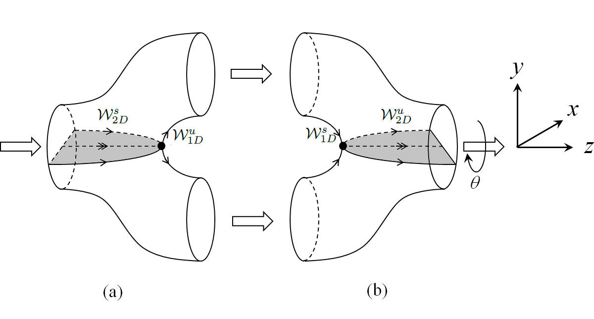
Figure 6: Schematic of pore branch (a) and merge (b) depicting stagnation points and associated 2D unstable $\mathcal{W}^{U}_{2D}$ and stable $\mathcal{W}^{S}_{2D}$ manifolds which act as surfaces of transverse minimum transverse flux. Note fluid stretching transverse to these surfaces and the orientation angle $\theta$ between these surfaces. Adapted from [25]

.

These stretching dynamics are shown schematically in the 3D baker’s flow depicted in Figure 7, adapted from [7], which corresponds to the case $\theta=\pi/2$. This schematic depicts fluid deformation (as illustrated by the dark/light bands) over a pore branch and subsequent merger, followed by a repeated branch and merger, under steady flow conditions. Whilst not shown, saddle-type stagnation points occur at each of the pore branches and mergers, and the associated 2D unstable manifolds project into the fluid bulk oriented at $\theta=\pi/2$ to each other, where the “twist” between the branch and merger is necessary to achieve this angle. The input flow (at left, $\phi_{0}$) is partitioned into two (light and dark) tones; after passing through two successive branch and merger re-arrangements, the fluid tones are re-distributed into an array of eight contiguous light and dark tones (at right, $\phi_{2}$), indicating that significant stretching and folding process has taken place along the flow trajectory. As per Figure 7, the 3D baker’s flow generates 2D fluid striations (sheets) which are stretched and thinned exponentially with the number $n$ of pore branches and merges as $2^{n}$. Numerical simulations [7] of Stokes flow in this geometry calculated that the Lyapunov exponent $\lambda_{\infty}\approx 0.68$ for this flow is withing 2% of the theoretical upper bound $\lambda_{\infty}=\ln 2$ for continuous steady 3D flows. Hence fluid stretching arising from pore branches and merges in certain geometries can generate very efficient mixing from chaotic advection. Note that these Lyapunov exponents are calculated with respect to the number $n$ of coupled pore branches and mergers rather than the time $t$ in (2).

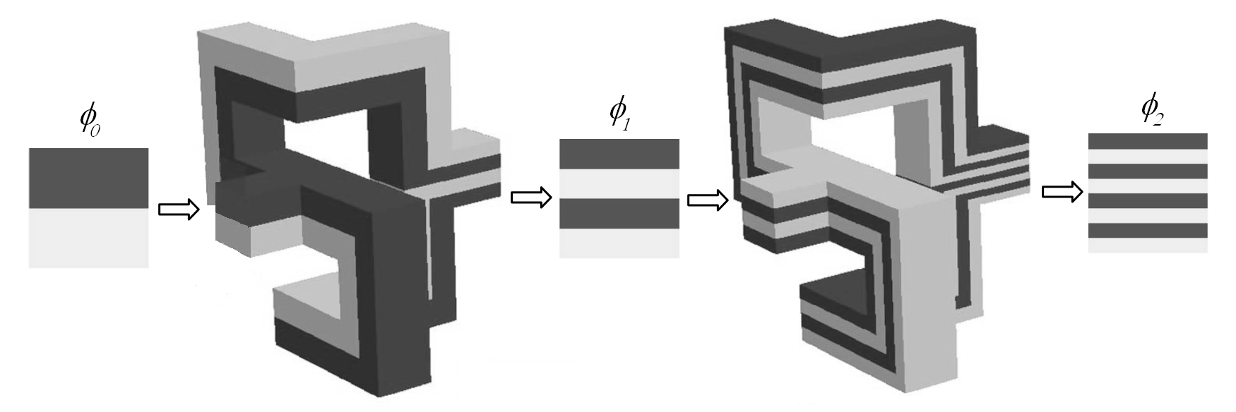
Figure 7: Schematic of the baker’s flow, a 3D fluid mechanical implementation of the baker’s map arising from non-trivial pore branching and merging. Adapted from [7].

For random porous media, the orientation angle $\theta$ is not at the optimum value $\theta=\pi/2$, but rather is randomly distributed (uniformly as an independent random variable) in the range $[0,\pi]$ between branches and mergers. For a random open porous network (detailed in Section 4) comprising randomly connected pore branches and mergers, the mean stretching rate was calculated in [25] to be $\lambda_{\infty}\approx 0.1178$. A schematic of the model connections in [25] is shown in Figure 8(a), and a typical macroscopic evolution of a dye plume continuously injected into a single pore is shown in Figure 8(b). Chaotic advection inherent to this open porous network rapidly organises these non-diffusive particles into highly striated material distributions which grow exponentially as $\ell(n)=\ell_{0}\exp(\lambda_{\infty}n)$ as shown in Figure 9, which illustrates the cross-sectional distribution of fluid tracer particles in a single pore as they evolve with pore number $n$ under a mean advective flow. Whilst these striations do not stretch as rapidly as for the 3D bakers flow shown in Figure 7, the underlying mechanism leading to chaotic advection in the random porous network is identical, and is also intrinsically applicable to granular systems and fracture networks.

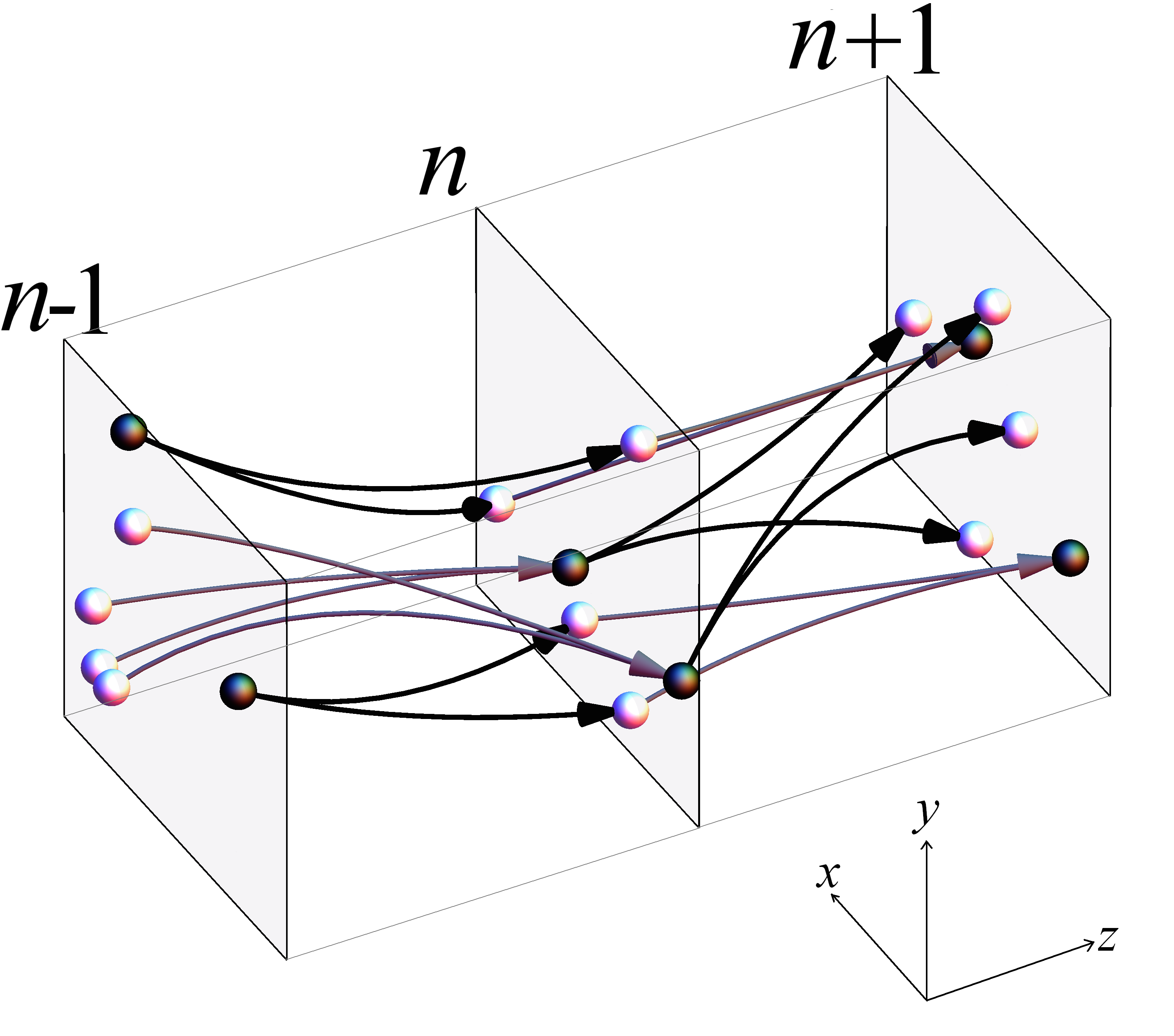
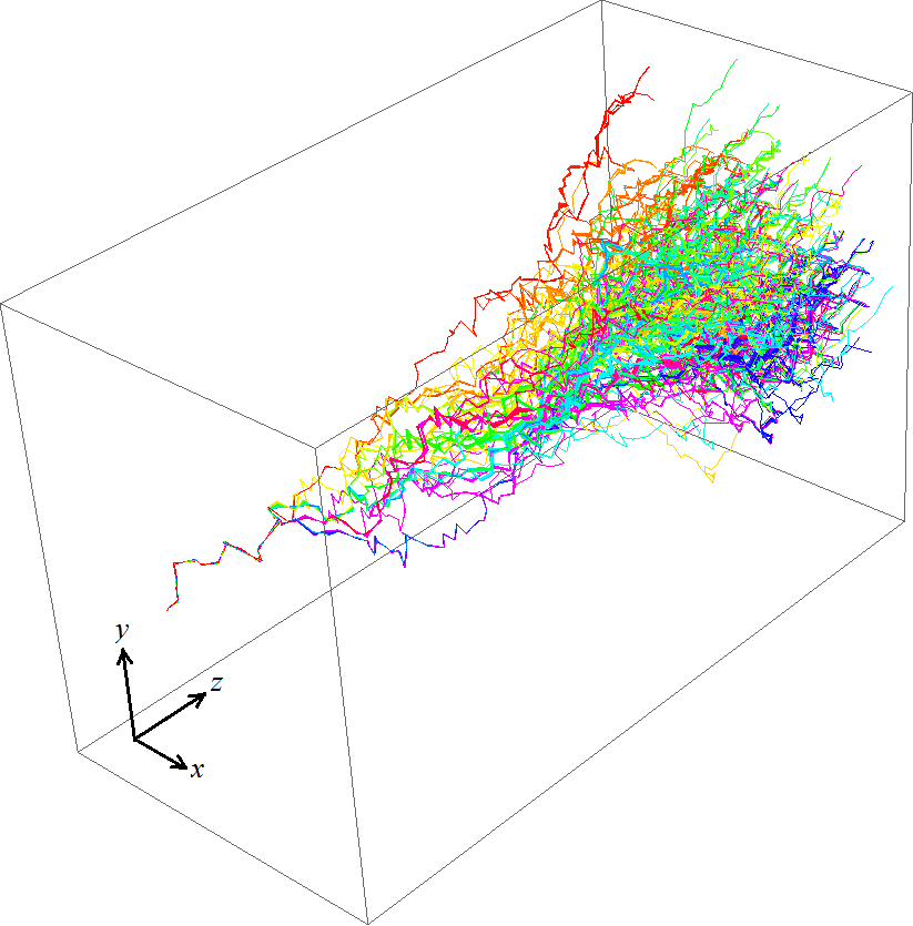
(a)	(b)

Figure 8: (a) Schematic of connectivity of pore branches (black) and mergers (white) between mapping planes in the open porous network model of [25], with branch pores (black) and merge pores (white) shown. (b) Evolution of a continuously injected line source of differently colored particles in a single pore within one realisation of the open porous network model.

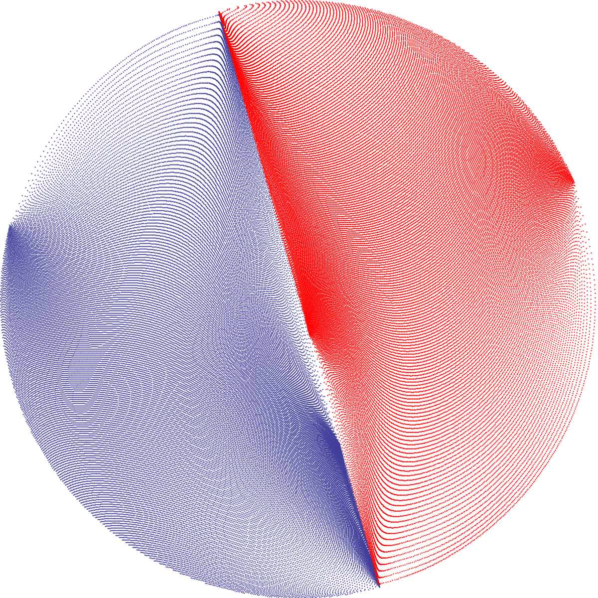
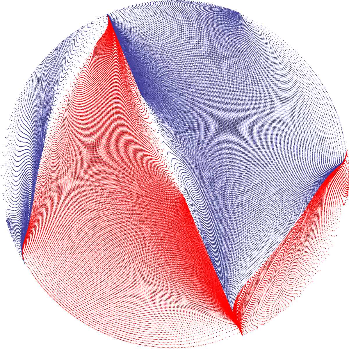
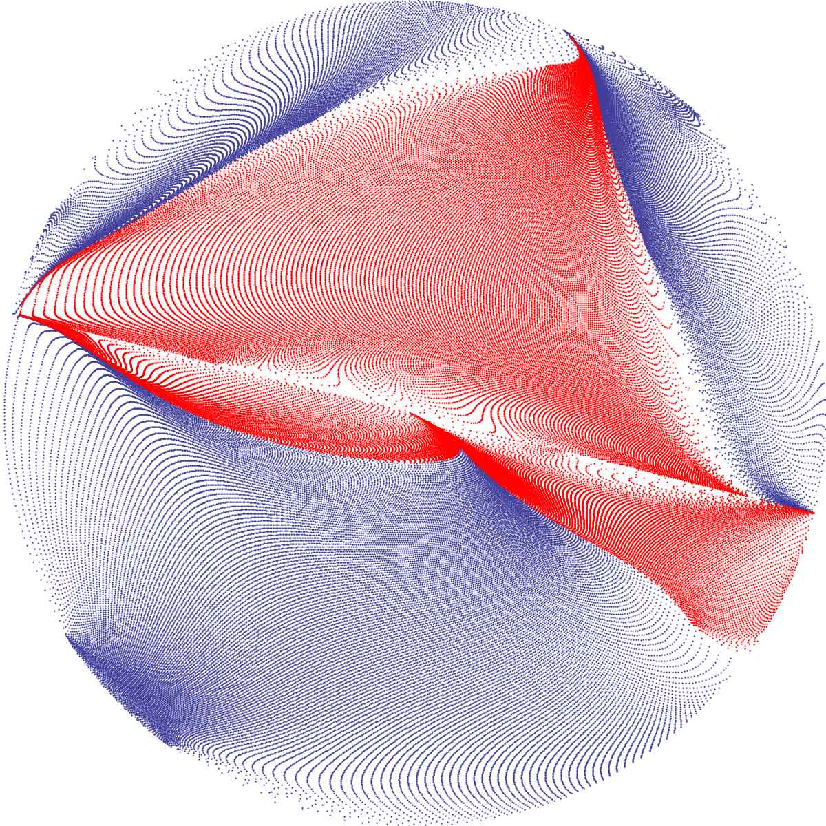
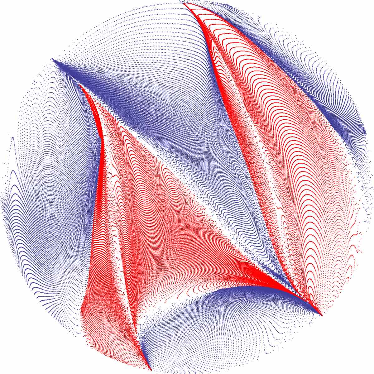
$n=1$	$n=2$	$n=6$	$n=8$
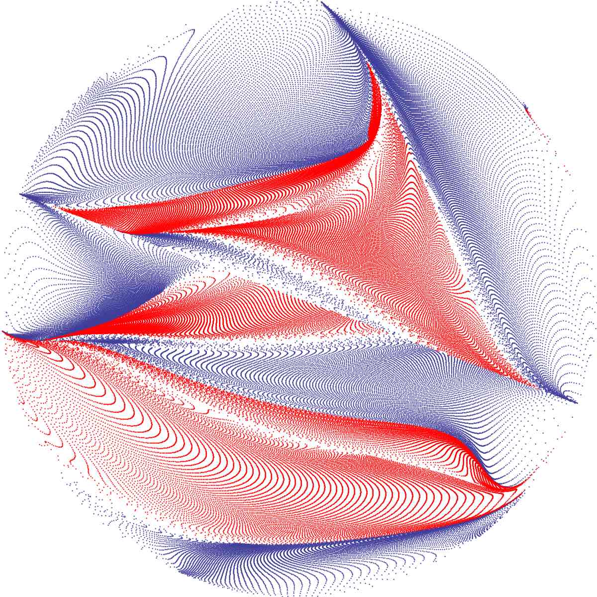
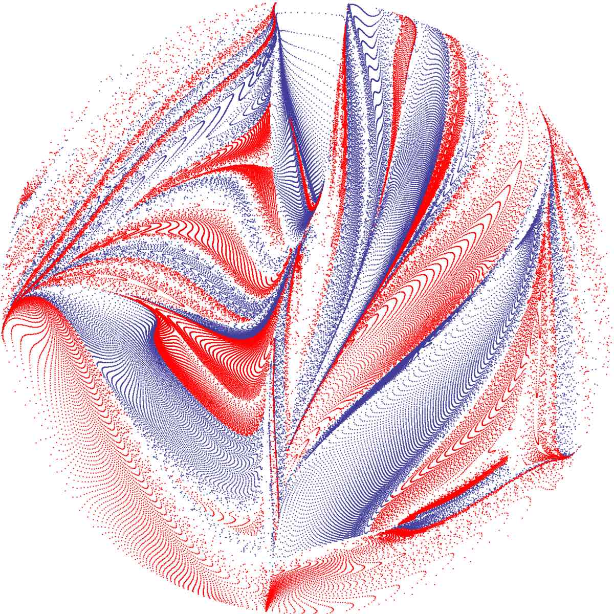
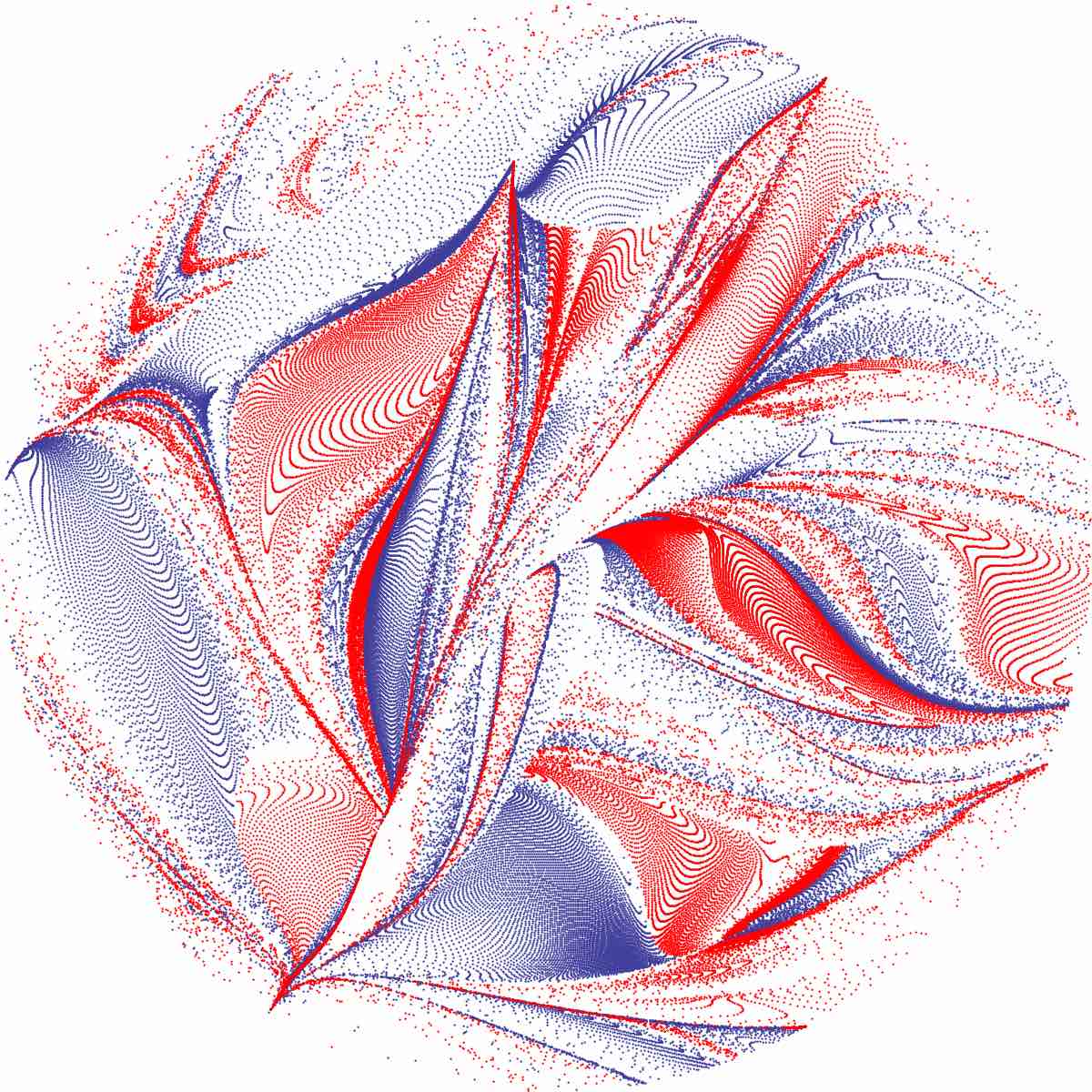
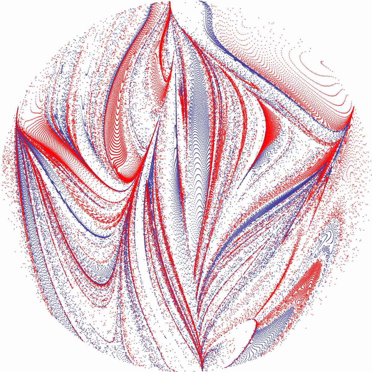
$n=10$	$n=20$	$n=30$	$n=40$

Figure 9: Typical evolution of coloured fluid particles with pore number $n$ in a 3D randomly oriented open porous network.

The ergodicity of streamline dynamics under chaotic advection means that the Lyapunov exponent $\lambda_{\infty}$ reflects both an ensemble average as well as a volumetric average. Although it may be surprising that fluid stretching in random porous media can lead to persistent exponential fluid stretching (as random stretching and compression may be expected to cancel), this persistence is explained by the asymmetry between fluid stretching and compression. Whilst material elements tend to align with the stretching direction and so amplify stretching, under compression material elements tend to align normal to the compression direction, hence compression is retarded. The Lyapunov exponent $\lambda_{\infty}\approx 0.1178$ directly quantifies this asymmetry.

Whilst significantly smaller than the upper bound $\lambda_{\infty}=\ln 2$, this mean stretching rate is still positive, which means that the topological complexity inherent to all porous media imparts significant chaotic advection to all 3D random media under steady flow conditions. As each branch and merge pair corresponds roughly to one pore (exactly in the model) and as significant mixing and spreading happens after a few tens of pore lengths (i.e. $l/l_{0}>100$ for $\lambda_{\infty}\approx 0.1178$ for $n>39$ pores), mixing and dispersion by chaotic advection is significant well within the averaging volumes typically associated with upscaling models: dispersion by chaotic advection cannot rightly be ignored when upscaling. Although the model used to develop these quantitative estimates is highly simplified, the fundamental properties (topological complexity and random pore orientation) are inherent to all 3D random porous media. Moreover, this rate presents a lower bound driven by the pore-space topology, and so does not account for for additional mechanisms such as surface roughness [41] and pore curvature [14]. Although fluid shear is also significant in all porous media (due to the important role played by the no-slip condition at grain surfaces), such mechanisms give rise only to algebraic fluid deformations, and so are dominated in the long term by the exponential fluid stretching associated with chaotic advection.

In this Section we have seen that there exist significant qualitative differences between the fluid dynamics in 2D and 3D porous media. In the latter case, complex streamline behaviour driven by the pore-scale topology generates chaotic advection, resulting in highly striated, lamellar material distributions which have the potential to accelerate pore-scale mixing and augment macroscopic transport. In the following Sections we explore the impact of these dynamics upon pore-scale transport and mixing which manifest as macroscopic dispersion and dilution.

4 Flow and transport in a model open porous network

To study the fundamentals of chaotic advection and transport in 3D random porous networks, we consider an idealised random model network based on the symmetric pore branch element $\Omega$ (shown in Figure 6(a)) which contains the minimum topological complexity and disorder common to all random porous media, i.e. branching and merging pores. This ideal network is homogeneous and isotropic at the macroscale, loosely defined as the length scale significantly greater than the characteristic length scale of $\Omega$. Whilst real porous media exhibit significantly more complexity in the pore-scale structure including features such as tortuosity, heterogeneity and surface roughness, for clarity of exposition we seek the simplest model which exhibits chaotic advection and anomalous transport. These phenomena persist in the presence of additional pore-scale features outlined above [26], which only act to alter the quantitative aspects of transport and dispersion. As the network model considered herein is the simplest representation of porous media with non-trivial pore-scale topology (which is common to all porous media), we contend that the qualitative transport dynamics of this model are universal. In Section 7 we demonstrate how these results can be extended to real porous architectures as characterised by e.g. micro-CT imaging.

The fundamental building block of the random network model is the symmetric pore branch element $\Omega$ (Figure 6(a)), and its reflected image given by the pore merge element (Figure 6(b)). A random continuous 3D network can be constructed by spatial composition of these branch and merge elements, as described in greater detail in A. Each random composition is unique, and a set of compositions forms an ensemble of random networks over which one can study the characteristics of scalar transport. The set of pore locations in each composition defines a realization of a 3D open porous network, and the set of all realizations of the porous network forms a statistical ensemble which is both ergodic and stationary. If the pore locations are uniformly and independently distributed (up to constraints of non-overlapping pores), then the resultant distribution of of the relative orientation of pairs of branches and merges $\theta$ is also uniform and independent. Hence transport within the 3D open porous network follows a multidimensional Markov process in space, forming a basis for the development of continuous-time random walk (CTRW) models of transport, deformation and mixing.

To model flow within the porous network, we consider the steady fluid velocity field $\mathbf{v}(\mathbf{x})$ within the pore branch element $\Omega$ given by Stokes law

$$\mu\nabla^{2}\mathbf{v}+\nabla p=0,\,\,\nabla\cdot\mathbf{v}=0,$$ (5)

forced by the pressure differential $\Delta p$ over the inlet and outlet pores, subject to the no-slip boundary condition $\mathbf{v}|_{\partial\Omega}=0$. The flow field within $\Omega$ is calculated numerically to order $10^{-16}$ accuracy using the finite-volume computational fluid dynamics (CFD) package ANSYS-CFX 14, and the resultant fluid streamlines, velocity and residence time distributions are shown in Figure 10(a)-(c). Figure 10(d) depicts detail of a saddle-type stagnation point at the pore branch in $\Omega$, the associated skin friction vector and stable manifold $\mathcal{W}^{S}_{2D}$ which acts as a minimal flux surface. Due to reversibility of Stokes flow, the deformation, fluid velocity and skin friction fields in the pore merge element are identical to that shown in Figure 10 with the velocity and skin friction field reversed, and so in this case the 2D manifold associated with the saddle-type reattachment point is an unstable manifold $\mathcal{W}^{U}_{2D}$.

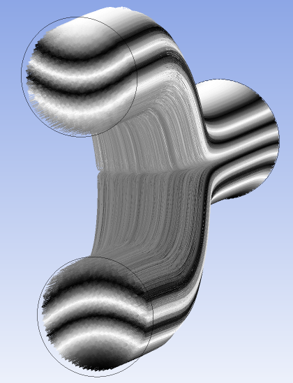
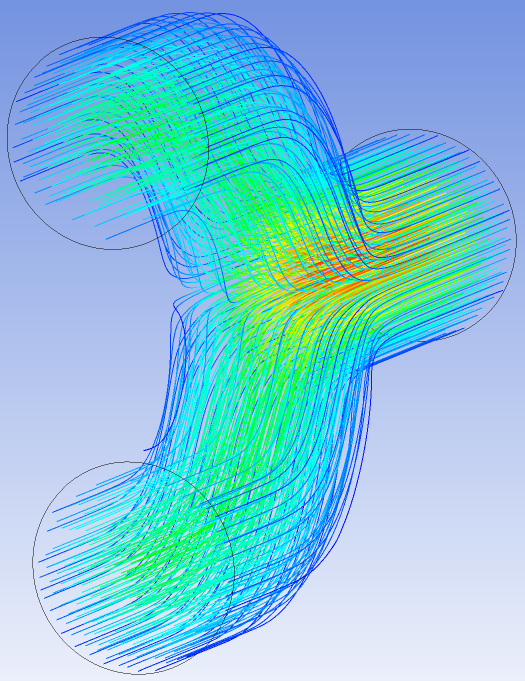
(a)	(b)
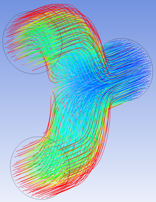
(c)	(d)

Figure 10: (a) Streamlines, (b) velocity, and (c) residence time distributions along streamlines under Stokes flow within the pore branch element $\Omega$ calculated from CFD calculations. (d) Saddle-type stagnation point (black dot), associated stable manifold $\mathcal{W}^{S}_{2D}$ (grey surface) and local skin friction vectors.

To generate a global transport model for the random porous network, we consider the effect on position and time of a fluid particle advecting through the pore branch and merge elements. We take the results shown in Figure 10 and define a transformation $\mathcal{M}^{\star}$ which maps advection of fluid particles from position $\{x_{r},y_{r}\}$ at the inlet pore of $\Omega$ to the outlet pore position $\{x_{r}^{\prime},y_{r}^{\prime}\}$, where $\{x_{r},y_{r}\}$, are the scaled and reoriented (by angle $\theta$) $x,y$ particle positions relative to the pore boundary at the inlet and outlet, such that $x_{r}^{2}+y_{r}^{2}=0,1$ corresponds to the pore centre and boundary respectively. Similarly, a temporal map $\mathcal{T}^{\star}:t\mapsto t^{\prime}$ quantifies the residence time $t^{\prime}-t$ along each particle streamline in $\Omega$. Distributions of exit positions $x_{r}^{\prime}$, $y_{r}^{\prime}$ and residence times $t^{\prime}-t$ are shown in Figure 11(a)-(c) for 100,000 streamlines within each branch element. The exact maps $\mathcal{M}^{\star}$, $\mathcal{T}^{\star}$ are remarkably well approximated (within relative error $\epsilon\sim 10^{-3}$) by the simple analytic maps $\mathcal{M}$, $\mathcal{T}$ (whose associated distributions are shown as contours in Figure 11(a)-(c))

$$\mathcal{M}:\{x_{r},y_{r}\}\mapsto\{x_{r},2y_{r}-\frac{|y_{r}|}{y_{r}}\sqrt{1-x_{r}^{2}}\},$$ (6)

$$\mathcal{T}:t\mapsto t+\frac{1}{1-x_{r}^{2}-y_{r}^{2}}.$$ (7)

Similarly, transport in a pore merge element is quantified by the inverse spatial map $\mathcal{M}^{-1}$. The no-slip boundary condition in $\Omega$ generates the residence time distribution (7) similar to that of a Poiseuille flow, which is singular at the pore boundary, leading to unbounded residence time distributions which, as shall be shown, have a significant impact upon transport and mixing. From (6), (7), the residence time in the pore branch and merge is quantified respectively by the composite operators $\mathcal{T}\circ\mathcal{M}$, $\mathcal{T}\circ\mathcal{M}^{-1}$, respectively. For randomly oriented branch and merge elements within the porous network, advection is quantified by the composite reoriented maps respectively as

$$\mathcal{S}(\theta) :=R(\theta)\circ\mathcal{M}\circ R(-\theta),$$ (8)

$$\mathcal{S}^{-1}(\theta) :=R(\theta)\circ\mathcal{M}^{-1}\circ R(-\theta),$$ (9)

where $R(\theta)$ is a reorientation operator. These composite advection operators reflect symmetry breaking for $\theta\neq 0$ over a coupled pore brach and merger such that

$$\mathcal{S}(\theta_{1})\circ\mathcal{S}^{-1}(\theta_{2})\neq I\,\,\text{for}\,\,\theta:=\theta_{1}-\theta_{2}\neq 0,$$ (10)

where $I$ is the identity operator. The approximate maps $\mathcal{S}(\theta)$, $\mathcal{T}$, capture the salient features of fluid stretching at stagnation points and hold-up at the no-slip boundaries of $\Omega$, and from Figure 11 accurately represent advection in the pore branch and merge elements. When appropriately concatenated, these maps permit highly efficient modelling of transport and mixing over a given realization of the open porous network.

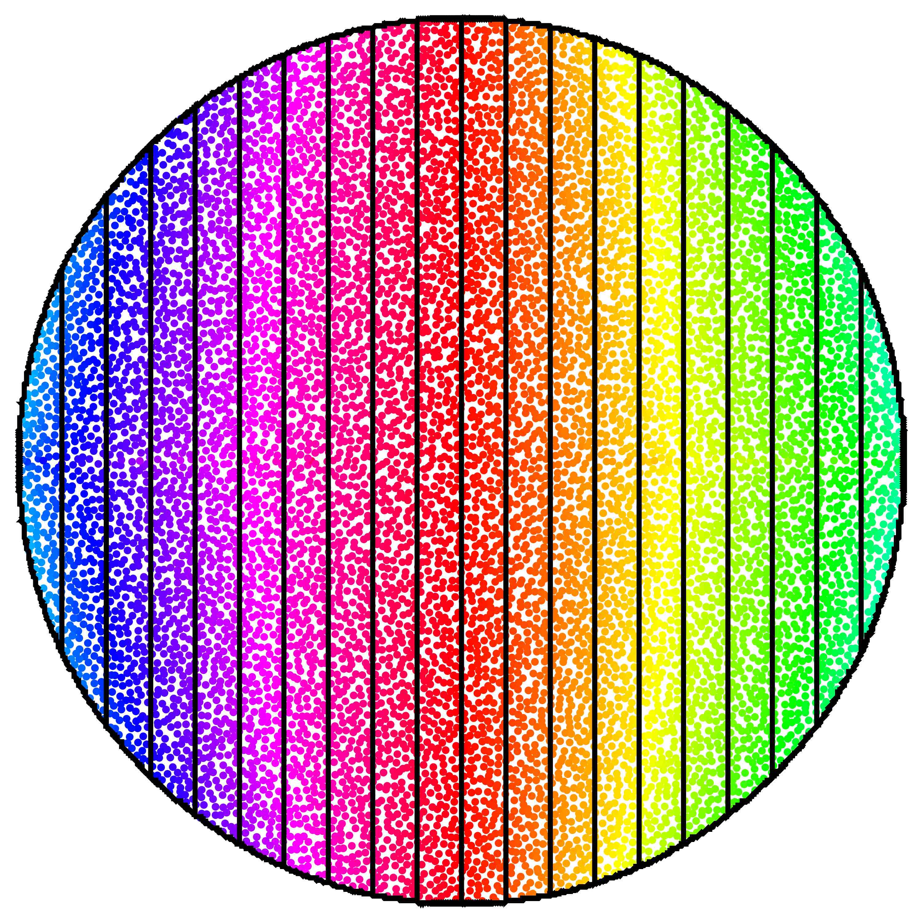
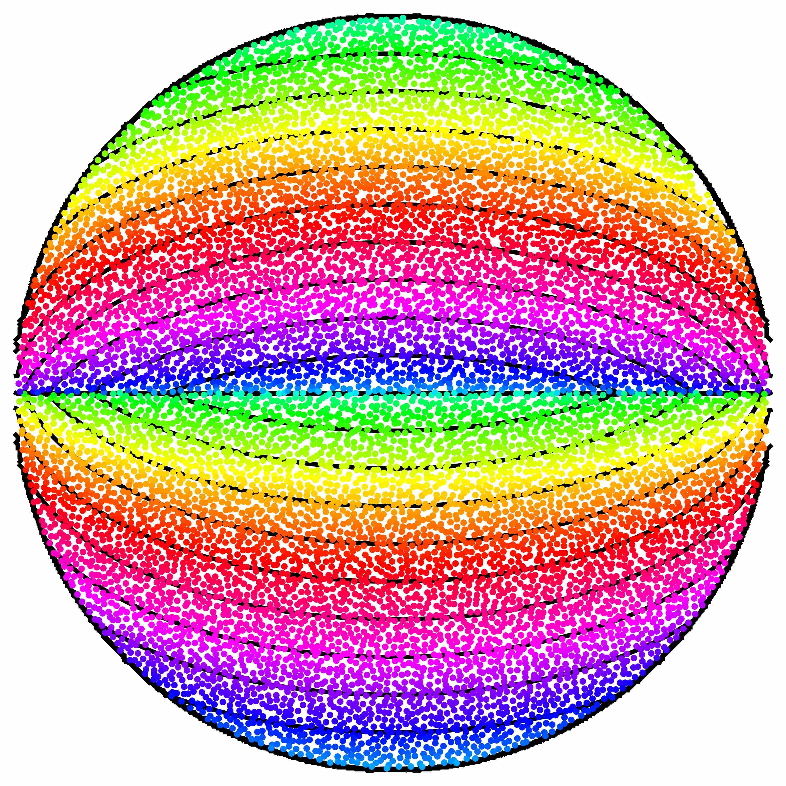
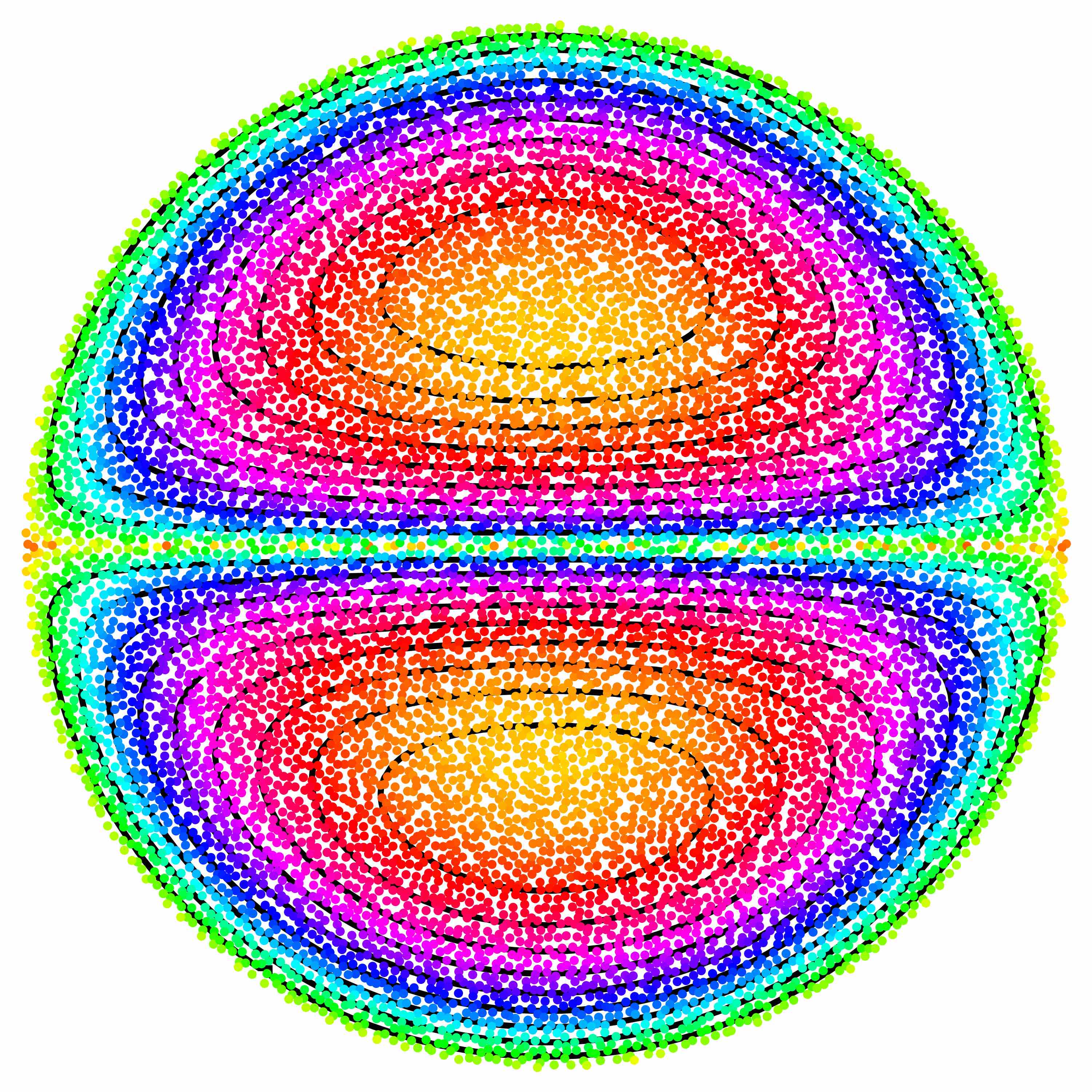
(a)	(b)	(c)

Figure 11: Comparison of distributions of (a) $x$-location, (b) $y$-location and (c) residence time in pore branch element $\Omega$ between CFD calculations (colored points) and approximate analytic maps $\mathcal{M}$ (6), $\mathcal{T}$ (7) (contour lines).

Macroscopic transport in a single realization of the pore network model is illustrated in Figure 8(b), where 1000 closely spaced (equidistant over a line 1/10th of the pore diameter) fluid particles (differentiated by colour) are advected over 100 pore branches and mergers in the absence of molecular diffusion. Transverse fluid stretching acts to initially spread these particles over the first 10 pores, as illustrated by a slight broadening of the particle trajectories, but after 10 pores the plume is split into several different pores, a process which repeats along the network, leading to macroscopic transverse dispersion which converges toward a Gaussian distribution of particles, reflecting the macroscopically homogeneous nature of the network. This behaviour clearly depicts how pore-scale chaotic advection impacts transverse dispersion; whilst macroscopic transverse dispersion is chiefly governed by the geometry and topology of the network, pore-scale chaotic advection acts to transversely stretch fluid elements, increasing the probability of bifurcation over a stagnation point and advection down different pores, leading to macroscopic dispersion. Hence chaotic advection does not alter the qualitative nature of transverse dispersion in homogeneous media, but rather impacts the rate of dispersion. However, as shall be shown, chaotic advection plays a significant role with respect to both longitudinal dispersion and mixing and dilution [17] within a plume.

Figure 9 shows the evolution of a dye trace simulation (consisting of the advection of a large number of diffusionless particles) propagated by the composite maps following a single pore through a realization of the random network (where the half blue/half red distribution of points is initiated across all pores), illustrating the formation of exponentially elongated material striations as the fluid approaches the well-mixed state. This behaviour is ubiquitous across all realizations of the random network, and non-mixing regions can only arise in ordered networks. Whilst there is no clear evidence of the folding of fluid elements in the $xy$-cross sections in Figure 9, folding occurs in the $z$-direction as fluid elements flow over stagnation points, and so manifests as discontinuities when projected into the $xy$-plane. The spatial and temporal maps $\mathcal{S}$, $\mathcal{T}$ implicitly capture this behaviour through the advection and residence time distributions.

Evolution of the residence time distribution for these points is shown in Figure 12, where the large residence times of the temporal map $\mathcal{T}$ associated with the no-slip boundary condition are clearly illustrated for small values of the longitudinal pore number $n$. The spatial distribution of residence times become increasing striated as particles are propagated through the network, and so chaotic advection acts to “mix” these residence times, as shown for large $n$, i.e. the residence time distribution in pores becomes more and more peaked and uniform, albeit retaining a long tail in the distribution. Whilst, in the absence of diffusion, particle trajectories and hence residence times are not random, the space-filling nature of chaotic orbits renders these trajectories to be ergodic, and so may be conceptualised as a random process with decaying correlation along streamlines, where this decay rate is directly related to the Lyapunov exponent $\lambda_{\infty}$. As shall be shown, the impact of such “mixing” of residence times has a significant impact upon macroscopic longitudinal dispersion.

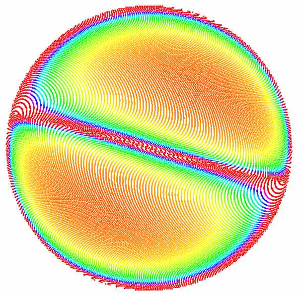
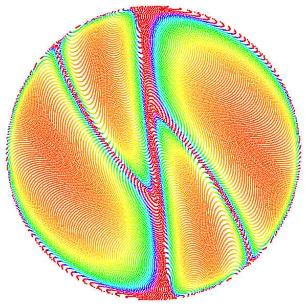
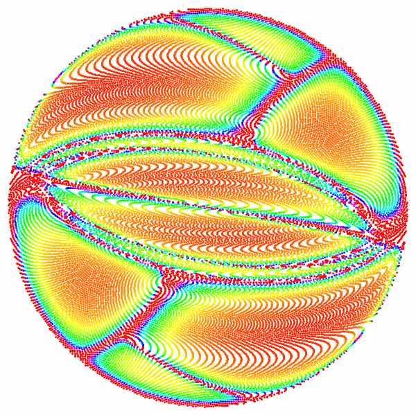
$n$=1	$n$=2	$n$=5
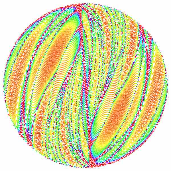
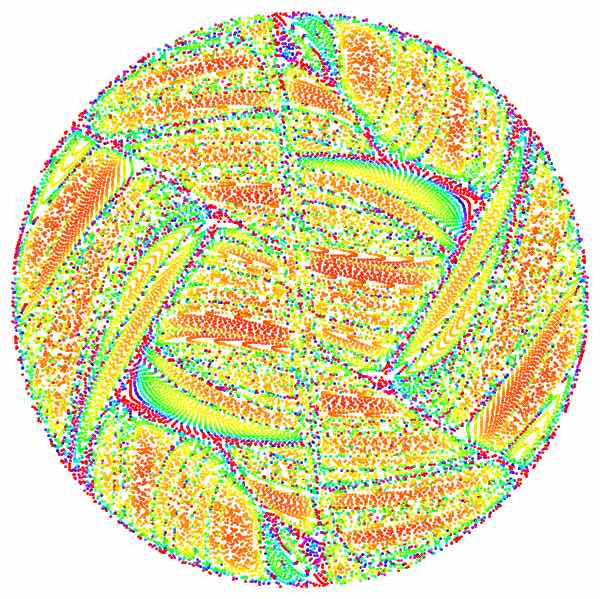
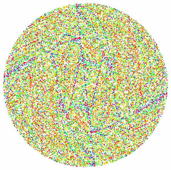
$n$=10	$n$=20	$n$=50

Figure 12: Calculated residence time distributions (pink = large, orange=small) with increasing number of pore branch-merge transitions $n$.

5 Pore-scale mixing due to chaotic advection-diffusion

The results above illustrate the mechanisms which generate chaotic advection in 3D porous media and the consequent impacts upon fluid stretching and material distributions. To quantify the impact of chaotic advection upon pore-scale mixing of a tracer solute, we summarise the results of Lester et al. [28] regarding the interplay of such fluid deformation with molecular diffusion. For simplicity of exposition we consider the steady concentration field $c(\mathbf{x})$ which arises from a continuous source at the inlet plane $z=0$ which is uniformly injected across all inlet pores as a line source with Gaussian concentration profile (given by (16)). Whilst this inlet condition is not representative of any physically important situation, this condition renders the macroscopic concentration distribution uniform and so more clearly illustrates the mixing and dilution dynamics. Results derived for this specific condition are then generalised to an arbitrary inhomogeneous macroscopic concentration distribution at the end of this section.

The concentration distribution within the pore space is described by the steady 3D advection-diffusion equation (ADE)

$$-\mathbf{v}(\mathbf{x})\cdot\nabla c(\mathbf{x})+D_{m}\nabla^{2}c(\mathbf{x})=0,$$ (11)

subject to the zero-flux boundary condition $\mathbf{n}\cdot\nabla c|_{\partial\mathcal{D}_{f}}=0$, where $\mathbf{n}$ is the outward normal vector from the fluid domain $\mathcal{D}_{f}$, and where $D_{m}$ is the molecular diffusivity. Following [28] we ignore longitudinal diffusion for the continuous injection protocol and thus pose the steady 3D ADE (11) as a transient 2D ADE in the $xy$-plane as

$$\frac{\partial c}{\partial t}=v_{z}\frac{\partial c}{\partial z}=-\mathbf{v}_{\bot}(x,y,t)\cdot\nabla_{\bot}c(x,y,t)+D_{m}\nabla^{2}_{\bot}c(x,y,t),$$ (12)

where $v_{z}$ is the $z$-component of $\mathbf{v}(\mathbf{x})$, $\mathbf{v}_{\bot}$ and $\nabla_{\bot}$ denote the $xy$-components of velocity and gradient operator respectively. The $z$-coordinate is also parameterised in terms of the Lagrangian travel time $t=t(z)$ along a given fluid particle trajectory as

$$t(z)=\int_{0}^{z}dz^{\prime}\frac{1}{v_{z}(z^{\prime})}.$$ (13)

Whilst the travel time $t(z_{0})$ for fixed $z=z_{0}$ also varies over the $xy$-plane, (12) provides a convenient basis for solution of the concentration field based upon a CTRW for the local advection time and deformation history of fluid elements.

For highly striated, lamellar material distributions (such as those generated by chaotic advection) the ADE simplifies to a 1D transport equation [38, 10, 11, 20] for an individual lamella l in terms of the material coordinates $\{\chi,\eta\}$ where $\eta$ is the coordinate transverse to the elongated lamella l and $\chi$ is the coordinate along the lamella. Due to fluid stretching, concentration gradients along the lamella ($\chi$) are exponentially weakened, whilst gradients transverse to the lamellae ($\eta$) are exponentially amplified, and so (12) further simplifies to

$$\frac{\partial c}{\partial t}-\gamma(t)\eta\frac{\partial c}{\partial\eta}=D_{m}\frac{\partial^{2}c}{\partial\eta^{2}},$$ (14)

where the temporal stretching rate of a lamella, $\gamma(t)$, is given by the elongation rate

$$\gamma(t)=\frac{d\ln\rho(t)}{dt},$$ (15)

and $\rho(t)=\ell(t)/\ell(0)$ is the local deformation of a material line relative to its original length $\ell(0)$. The ensemble average of the stretching rate $\gamma(t)$ converges toward a constant for exponential stretching and scales as $1/t$ for algebraic fluid stretching, and so the fluid deformation rate directly impacts the evolution of the lamellae. For a Gaussian initial concentration profile in each pore of the form

$$c(\eta,0)=\frac{c_{0}}{\sqrt{2\pi\sigma_{0}^{2}}}\exp\left(-\frac{\eta^{2}}{2\sigma_{0}^{2}}\right),$$ (16)

solutions to the lamellar ADE (14) are given by

$$c(\eta,t)=\frac{c_{0}}{\sqrt{2\pi(\sigma_{0}^{2}+2D_{m}\tau(t))}}\exp\left(-\frac{\eta^{2}\rho(t)^{2}}{2\sigma_{0}^{2}+4D_{m}\tau(t)}\right),$$ (17)

where the maximum concentration across the lamella is $c_{m}(t)=c(0,t)$ and the operational time $\tau(t)$ which encodes the entire stretching history is defined as

$$\tau(t)=\int_{0}^{t}\rho(t^{\prime})^{2}dt^{\prime}.$$ (18)

Hence the action of fluid stretching as quantified by $\rho(t)$ acts to both narrow the striation due to fluid stretching, but also increase the profile variance as $\sigma^{\star 2}(t)=\sigma_{0}^{2}(t)+2D_{m}\tau(t)$. Note that (17) quantifies the transverse concentration profile at a single point along the lamellar backbone (denote by the $\chi$-coordinate), and so the concentration field over a single is described as $c(\chi,\eta,t)$. The entire concentration field is then comprised of the set of lamellae undergoing distortions as they migrate through the pore-space.

To develop analytic solutions for the evolving concentration field, Lester et al. [27] develop a stretching CTRW in the open porous network which describes evolution of fluid deformation with pore number $n$ as a two-step process (corresponding to alternating pore branches and mergers) for the advection time $t$ and length $\ell$ (in the $\chi$-direction) of an element of a material strip (lamella) in the 2D plane transverse to the mean flow direction as

$$\ell_{n+1}=\ell_{n}\rho_{s}(\varphi_{n}),\quad\quad t_{n+1}=t_{n}+\Delta t_{n},$$ (19)

$$\ell_{n+2}=\ell_{n+1}\rho_{c}(\varphi_{n+1}),\quad\quad t_{n+2}=t_{n+1}+\Delta t_{n},$$ (20)

where $n$ is the pore number and $\Delta t_{n}$ is the advection time between pores. $\rho_{s}(\theta)$, $\rho_{c}(\theta)$ are the relative elongations due to stretching and compression, respectively, of $\ell$ over a pore branch and merger, and $\varphi$ is the orientation of the material strip with respect to the pore branch or merger which, due to randomness of the pore network, is distributed uniformly over $[-\pi,\pi]$. Note that $\theta$ represents the angle between a pore branch and merger, whereas $\varphi$ represents the angle between the material strip and the local branch or merger. Closed expressions for the relative elongations $\rho_{s}$, $\rho_{c}$ are derived directly from the advection maps $\mathcal{S}(\theta)$, $\mathcal{S}^{-1}(\theta)$ as

$$\rho_{s}(\varphi)=\sqrt{1+3\cos^{2}\varphi},$$ (21)

$$\rho_{c}(\varphi)=\frac{1}{2}\sqrt{4-3\cos^{2}\varphi}.$$ (22)

Similarly, the distribution of advection time between pores $\Delta t_{n}$ determined from the temporal map $\mathcal{T}$ is distributed as a Pareto variable

$$\psi(\Delta t)=H(\Delta t-\Delta t_{a})\frac{1}{\Delta t_{a}}\left(\frac{\Delta t}{\Delta t_{a}}\right)^{-2},$$ (23)

where $H$ is the Heaviside step function and $\Delta t_{a}$ is the minimum waiting time in the pore. As discussed above, the ergodicity of chaotic orbits permits the space-filling nature of fluid particle trajectories to be modelled as the stochastic process defined by equations (19) and (20). This stretching CTRW captures the essential features of exponential fluid stretching and arbitrarily long waiting times as the fluid particles propagate through the porous medium. As a result of the Central Limit Theorem, the total fluid deformation $\rho=\rho_{s}\rho_{c}$ over a coupled pore branch/merger converges with pore number $n$ toward a lognormal distribution

$$\hat{p}_{\rho}(\rho)=\frac{1}{\rho\sqrt{\pi n\sigma^{2}}}\exp\left[-\frac{(\ln\rho-n\lambda_{\infty}/2)^{2}}{n\sigma^{2}}\right],$$ (24)

where the asymptotic average stretching rate $\lambda_{\infty}\approx 0.1178$ and variance $\sigma^{2}\approx 0.11436$ over the pore network are derived from (21), (22). This result allows the evolution of the total deformation $\rho$ given by the two-step CTRW (19) (20) to be expressed in terms of of a one-step CTRW for the relative stretch $\rho_{n}$ of the line element as

$$l_{n+1}=l_{n}\rho_{n},\quad\quad t_{n+1}=t_{n}+\Delta t_{n},$$ (25)

which may be solved analytically [27]. To solve diffusive mixing in the pore network, it is necessary to also solve the operational time $\tau(t)$ in (17), which is well-approximated by the expression

$$\tau_{n}:=\tau(t_{n})\approx\frac{t_{n}\rho_{n}^{2}}{n\Lambda_{\infty}},$$ (26)

where $\Lambda_{\infty}=\lambda_{\infty}+\sigma^{2}$. These results completely quantify evolution of the lamellar mixing model (17) up to the coalescence regime, where previously non-interacting lamellae merge into a continuous mixing plume, and the 1D approximation governing (17) breaks down. Methods are available [10, 20] to predict evolution of the scalar concentration field beyond this coalescence limit, and whilst these are beyond the scope of this paper, the rate of mixing is still strongly dependent upon the fluid stretching dynamics, hence chaotic advection augments fluid mixing in this regime also.

As shown by Lester et al. [27] and Le Borgne et al. [21], this CTRW formulation leads to asymptotic estimates of the decline in average maximum concentration of the tracer plume as the pore number $n$ increases. In 2D porous networks, the asymptotic maximum concentration $c_{m}$ decays algebraically with $n$ as

$$\langle c_{m,2D}(n)\rangle\propto n^{-\alpha-\frac{\beta+1}{2}},$$ (27)

where $\alpha\geqslant 1/2$ and $\beta\leqslant 2$ are characteristic exponents of the underlying velocity distribution [9, 8]. However, in 3D porous networks the asymptotic maximum concentration declines exponentially with $n$ as

$$\langle c_{m,3D}(n)\rangle\propto\frac{1}{\sqrt{\ln(n)}}\exp\left[-n\frac{2\lambda_{\infty}+\sigma^{2}}{4}\right].$$ (28)

In terms of ergodic theory 2D steady porous media flows intrinsically produce, at best, weak mixing, and 3D steady porous media flows intrinsically produce strong mixing.

The fundamental difference between mixing in 2D and 3D porous media is clear. The Poincaré-Bendixson theorem [43] excludes chaotic advection in 2D steady flows but permits it in 3D steady flows. This phenomenon must occur and even be ubiquitous in topologically complex porous media. The major observable effect is a transition from algebraic fluid stretching in two dimensions to exponential stretching in three dimensions that leads to exponential dilution at the pore scale in real systems as a function of longitudinal distance(the pore number $n$) from a point source.

This behaviour is also observed in the rate of scalar dissipation (quantified as variance decay), where Lester et al [27] show that concentration variance across a pore of area $A$ varies with pore number $n$ directly as

$$\sigma_{c}^{2}(n):=\frac{1}{A}\int_{A}(c(\eta,t_{n})-\overline{c(n)})^{2}dA=\overline{c(n)}^{2}\left(\frac{\langle c_{m}(n)\rangle}{\sqrt{2}\,\overline{c(n)}}-1\right),$$ (29)

where $\overline{c(n)}$ is the average concentration across the pore and $\langle c_{m}(n)\rangle$ is the average concentration over the concentration support area, defined as the area corresponding to $c$ greater than an cut-off concentration $\epsilon$ which is small but finite [27]. For moderate $n$, where $\langle c_{m}(n)\rangle\gg\overline{c(n)}$, the scalar variance scales as $\langle c_{m}(n)\rangle$, and so the rate of fluid stretching directly impacts the rate of scalar dissipation. Again, the chaotic advection inherent to 3D porous media imparts dissipation which scales exponentially with pore number $n$, whereas algebraic dissipation obtains in 2D porous media.

These results are generalised in [27] to the case of an arbitrary heterogeneous macroscopic concentration distribution, which may be defined in terms of the total length $l_{p}(\mathbf{x})$ of lamellae per pore local to $\mathbf{x}$. For such a macroscopic distribution, the concentration mean and variance within the plume then vary as

$$\overline{c_{p}(\mathbf{x})}=\overline{c(n)}\frac{l_{p}(\mathbf{x})}{l(n)},$$ (30)

$$\sigma_{c_{p}}^{2}=\overline{c_{p}(\mathbf{x})}^{2}\left(\frac{\langle c_{m}(n)\rangle}{\sqrt{2}\overline{c_{p}(\mathbf{x})}}-1\right),$$ (31)

and again the rate of scalar dissipation within a heterogeneous plume is also governed by the rate of fluid stretching via $\langle c_{m}(n)\rangle$. Hence chaotic advection acts to significantly alter the dynamics of mixing and dilution at both the pore and macro scales.

6 Impact of chaotic advection upon longitudinal dispersion

In the previous Section we have considered the impact of pore-scale chaotic advection upon mixing and dilution. As illustrated in Figure 12, these kinematics also significantly impact evolution of the residence time distribution and hence longitudinal dispersion, as is well established over several studies [34, 13, 33, 22, 23] of chaotic duct flows. Pore-scale chaotic advection imparts particle trajectories which, whilst deterministic, are ergodic due to the space-filling nature of the chaotic orbits. Hence diffusion-less fluid trajectories sample all of the velocities across the pore space as they are advected downstream, retarding longitudinal dispersion in a manner similar to Taylor-Aris dispersion. Specifically, in the absence of diffusion, pore-scale chaotic advection acts to retard growth of longitudinal variance $\sigma_{L}^{2}(t)$ (related to longitudinal dispersion as $D_{L}(t)=\sigma_{L}^{2}(t)/2t)$ from ballistic growth $\sigma_{L}^{2}(t)\sim t^{2}$ due to the no-slip boundary condition to super-diffusive growth $\sigma_{L}^{2}(t)\sim t^{\alpha}$, $1<\alpha<2$. While analogous to Taylor-Aris dispersion in the presence of molecular diffusion, this mechanism is distinctly different in that chaotic advection is hydrodynamic (geometric) in origin and deterministic and so cannot be modelled as a simple Fickian diffusion process. These dynamics also persist in the presence of molecular diffusion in that chaotic advection provides a mechanism to significantly accelerate transverse mixing, which in turn further retards longitudinal dispersion [22, 23].

In this section we first quantify the impacts of pore-scale chaotic advection upon longitudinal dispersion in the absence of molecular diffusion, prior to discussion of extension of these results to diffusive tracers. Whilst chaotic orbits are not random, these fluid trajectories exhibit decaying correlations (the decay rate of which is related to the Lyapunov exponent $\lambda_{\infty}$), and so follow a Markov process when appropriately spatially discretised. This property allows diffusion-less tracer advection in the 3D open porous network to be modelled as a CTRW, which captures the interactions between tracer holdup due to the no-slip boundary condition and chaotic advection due to fluid stretching around stagnation points of the flow.

In Lester et al. [26] we formalized this CTRW in terms of the displacements $\Delta\mathbf{x}$ and transition times $\Delta t$ over each pore branch and merge element of the flow (shown in Figure 6) which are populated from the CFD computations outlined in Section 4. If we consider the evolution of a fluid particle propagating in the mean flow direction $z$, then in the absence of diffusion the longitudinal position $z$ and residence time $t$ of fluid particle evolves via the CTRW as

$$t_{n+1} =t_{n}+\Delta t_{n},$$ (32)

$$z_{n+1} =z_{n}+\Delta z,$$ (33)

where the temporal increment $\Delta t$ is distributed via the PDF $\psi(\Delta t)$ (23), and for the model network the spatial increment $\Delta z$ is constant (corresponding to the distance between mapping planes in Figure 8). Solution of this CTRW [26] shows that the axial distribution of fluid particles $p_{L}(n,t)$ (expressed in terms of longitudinal pore number $n$) rapidly converges to a Landau distribution $p_{l}(\tau)$

$$p_{L}(n,t) =\frac{2}{\pi}\left(\frac{1}{n}+\frac{t}{n^{2}}\right)p_{l}\left[\frac{2t-2n\left(\ln(n+1)-\gamma^{\star}-\ln\frac{2}{\pi}\right)}{n\pi}\right],$$ (34)

$$p_{l}(\tau) =\frac{1}{\pi}\int_{0}^{\infty}\exp(-\zeta\ln\zeta-\tau\zeta)\sin(\pi\zeta)d\zeta,$$ (35)

where $\gamma^{\star}$ is Euler’s constant. As shown in Figure 13(a), this prediction agrees well with direct numerical simulations via the advection and temporal maps $\mathcal{S}$, $\mathcal{T}$ for the open porous network. The asymptotic longitudinal variance of the resulting distribution is also estimated as

$$\sigma_{L}^{2}(t)\sim\frac{t^{2}}{(\ln t)^{3}},$$ (36)

which agrees well with predictions from the 3D pore network model at long times ($t\gtrsim 10^{3}$) (Figure 13(b)). Hence the impact of chaotic advection in the 3D model network is to retard longitudinal dispersion from a ballistic phenomenon $\sigma_{L}^{2}(t)\sim t^{2}$ to super-diffusive anomalous transport $\sigma_{L}^{2}(t)\sim t^{2}/(\ln t)^{3}$.

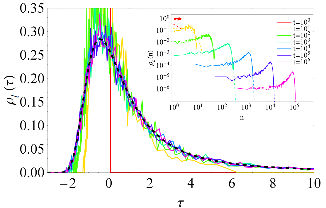
(a)

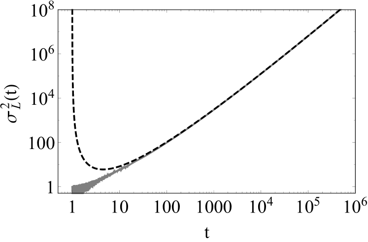
(b)

Figure 13: (a) (Color online) Convergence of residence time distribution for $10^{5}$ orbits in a single realization of the random network upon shifting and scaling to the Landau distribution $\rho_{l}(t)$. Inset: comparison between analytic (dashed) and numerical (solid) axial distribution $\rho_{L}(n)$. (b) Longitudinal dispersion $\sigma_{L}^{2}(t)\sim t^{2}/(\ln t)^{3}$ as predicted by asymptotic estimate in (36) (dashed, black) and pore network simulations (solid, grey).

For real homogeneous porous media the topology and geometry of the pore space is more complex than is catered for in the idealised 3D network that we use here for illustration. This difference would lead to alterations in the transverse stretching rates $\lambda_{\infty}$, and spatial $\rho_{\Delta x}$ and temporal $\psi(\Delta t)$ increments in the CTRW model. It is important to note that the Lyapunov exponent $\lambda_{\infty}$ does not directly control longitudinal plume dispersion; rather $\lambda_{\infty}$ ensures ergodicity of fluid orbits which renders the assumptions of the CTRW model valid, and so only the spatial and temporal increments control longitudinal dispersion. The asymptotic scaling result (36) holds for all $\rho_{\Delta x}$ under the Poiseuille (Pareto) time increment (23). In general, the CTRW longitudinal dispersion for any porous medium can be derived, given $\psi(\Delta t)$, $\rho_{\Delta x}(\Delta x)$. As discussed by Lester et al. [26], the no-slip boundary condition generates unbounded temporal increments $\psi(\Delta t)$ and, as a consequence, for any spatial increment distribution $\rho_{\Delta x}(\Delta x)$, the CTRW dynamics lead to pre-asymptotic and asymptotic transport which is universally anomalous (super-linear but sub-ballistic).

These results may also be extended to the case of diffusive tracers, where pore-scale chaotic advection acts to significantly accelerate scalar mixing, essentially enhancing the Taylor-Aris mechanism for molecular diffusion, and so further retarding longitudinal dispersion. In the presence of molecular diffusion, the asymptotic longitudinal dispersion dynamics are rendered Fickian, and so may be quantified solely in terms of an asymptotic dispersion coefficient $D_{L,\infty}$. These dynamics are most clearly illustrated via consideration of the mathematical connection between transverse mixing and RTD evolution in boundary-dominated flows [22]. In general, the rate of transverse mixing scales with Peclét number $Pe$ as $Pe^{\alpha}$, where $\alpha\approx 1/2$ for chaotic advection. The relationship between longitudinal dispersion and traverse mixing then yields [22, 23]

$$D_{L,\infty}=D_{m}\left(1+\kappa_{0}Pe^{2-\alpha}D_{m}\right),$$ (37)

In general, accelerated transverse mixing directly retards asymptotic longitudinal dispersion. Whilst diffusive longitudinal dispersion is yet to be couched in terms of stochastic models, the physical mechanisms are generic to all porous media, time scales and length scales, and have profound effects upon dispersion at the macroscale. Hence, pore-scale chaotic advection significantly augments dispersion and mixing at the macroscale in all porous media.

7 Application to Non-Ideal Porous Architectures

The pore-scale advection dynamics and implications for dispersion and mixing analysed in sections 4-6 are based upon idealised models of random porous media and leading-order analysis of the deformation dynamics and associated mixing phenomena. Whilst quantitative, these idealised models act to illustrate the governing mechanisms and resultant scalings for mixing and dispersion. To develop more general theories of macroscopic transport which capture the effects of more realistic pore-scale phenomena, it it necessary to extend these results to non-ideal media, such as pore space architectures given by micro-CT imaging studies.

Such an approach not only facilitates the development of stochastic models of mixing and dispersion which honour the pore-scale advection dynamics but also provide important data with respect to linking measures of pore-scale geometry (such as topology, tortuosity, heterogeneity) of real media to stochastic mixing kernels. This approach both identifies the pore-scale features which govern transport and mixing and paves the way for development of stochastic models which are couched directly in terms of medium properties. By utilising recent developments in lamellar mixing models [20, 21] for porous media which use deformation dynamics as inputs, it is possible to predict evolution of the full concentration PDF within the plume, which is important for upscaling of mixing and nonlinear chemical reactions.

Although exponential fluid stretching due to pore-scale chaotic advection dominates over algebraic deformation due to shear in the asymptotic limit, convergence to this regime may be slow, and so shear deformation can also play an important role in the pre-asymptotic regime. Moreover, fluid deformation (strain) is a tensorial, rather than scalar, quantity, and so to capture all of the augmented transport dynamics that arise from the interplay of molecular diffusion and fluid advection at the pore-scale it is necessary to properly quantify the full fluid deformation gradient tensor $\mathbf{F}$ which evolves along a streamline as

$$\frac{d\mathbf{F}}{dt}=[\nabla\mathbf{v}(t)]^{T}\cdot\mathbf{F}(t),\,\,\mathbf{F}(0)=\mathbf{I},$$ (38)

where the advection time $t$ denotes the position $\mathbf{x}(t)$ along a streamline with initial position $\mathbf{x}(0)=\mathbf{x}_{0}$.

This issue is illustrated by consideration of the difference between 3D fluid mixing under continuous or pulsed injection of a line source. Focusing solely upon the advection dynamics (i.e. ignoring diffusion), in the continuous injection case (as considered in Section 5) the line source forms a continuous 2D sheet which is stretched exponentially and folded into a 2D lamellar structure. Deformation of this sheet is governed by longitudinal and transverse stretching and shear, as quantified by the elements of $\mathbf{F}$. Conversely, transient injection of a line source (as considered in Section 6) at the same injection point generates a continuous 1D line which, at any point in time, resides within the 2D sheet described above. Whilst deformation of this 1D line evolves in a different manner to that of the 2D sheet, this evolution is also quantified by the elements of $\mathbf{F}$, albeit a different combination to that of the 2D sheet. As such, there is not a unique scalar stretching rate that characterises fluid deformation relevant to all transport phenomena but rather an evolving tensorial quantity, the elements of which are relevant for different initial and boundary conditions.

While pore-scale imaging provides topographic data for specific porous samples, it is necessary to develop stochastic models of dispersion and mixing from these datasets under appropriate assumptions of stationarity and ergodicity. This approach facilitates the development of upscaled transport models which both honour the pore-scale dynamics and are derived directly from the pore-scale architecture. This approach revolves around development of a CTRW model of fluid deformation, the stochastic kernels of which are populated from pore-scale computational fluid dynamics simulations. This approach is supported by observations over several different 2D and 3D steady flow fields [18, 19, 23] that fluid advection (and hence deformation) follows a spatial Markov process along fluid streamlines. Given computation of the steady fluid velocity field $\mathbf{v}$ and velociy gradient $\nabla\mathbf{v}$ to sufficient precision over the pore-space, the fluid deformation evolves as per (38).

Recent studies [28, 23, 9] have shown that by rotation of (38) into a streamline coordinate system, the fluid deformation evolution equation (38) takes on a particularly simple form, and permits explicit solution in terms of a CTRW along fluid streamlines. As the elements of the velocity gradient in this frame are almost fully independent and Gaussian distributed for random flows [28], stochastic models for the evolution of $\mathbf{F}(t)$ can be directly determined from pore-scale fluid dynamics simulations. This stochastic characterisation of tensorial fluid deformation generates a richer dataset than is given by, for example, the Lyaponuv exponent or algebraic stretching rate alone, and so can be used as inputs for lamellar-based models of dilution and mixing relevant to various transport phenomena.

Under this approach, exponential fluid stretching due to pore-scale chaos is captured along with shear deformation due to viscous flow, facilitating characterisation of mixing and dispersion in both the pre-asymptotic and asymptotic regimes. The development permits application of lamellar mixing models [11, 21] to predict evolution of concentration PDF within a solute plume, as well as augmented longitudinal and transverse dispersion which explicitly capture the deformation dynamics inherent to the porous architecture. These stochastic models automatically capture pore-scale chaotic advection, and facilitate the development of quantitative linkages between pore-scale geometry (such as topology, tortuously, heterogeneity etc) and the stochastic kernels. In the absence of such tools, it is difficult to envisage how to process the large datasets associated with CFD modelling of pore-scale geometries beyond direct simulation of transport and mixing in the specific porous architectures at hand. Stochastic modelling of fluid deformation and lamellar mixing addresses this need and thus provides the building blocks for upscaling methods for mixing and transport which explicitly honour both the pore-scale deformation dynamics and architecture.

8 Conclusions

There is considerable empirical evidence dating back to the 1960’s to show that the mixing and spreading of solute plumes as they travel through saturated porous media display unexpected dynamics and statistics, at both short and long travel times. Early researchers sought to reconcile these characteristics by identifying upscaled (’effective’) quantities at the representative elemental volume (REV) scale or larger, e.g. macrodispersivities, bulk reaction rates etc. While consistent with the underlying picture of (laminar) Darcian flow at the meso- and macroscale, these approaches neglected the complexity of fluid dynamics at the pore scale in favour of unduly homogenized descriptions. In recent years, as observation and computational techniques have advanced, it has become possible to study transport processes at the pore scale and to embark upon quantitative upscaling efforts to support estimation of effective parameters at the macroscale. Even so there is a richness of physics operating at the pore scale that can be overlooked in the rush to find robust upscaling methodologies.

We have demonstrated in this paper that even steady, non-turbulent flows must engender chaotic (space-filling) fluid trajectories in all 3D random porous media, with an idealized 3D random pore network as an illustrative example. This profound result is a consequence of the topological complexity inherent to all porous media and presents a fundamentally new genesis for observed microscale plume spreading, that has previously been categorized as mechanical dispersion generated by streamline branching, as depicted in Figure 1. Indeed, kinematically speaking, the process of steady streamlines separating around grain boundaries cannot lead to persistent plume spreading in 2D and, as was shown in this work, persistent spreading can only be generated by steady continuum flows in 3D. Chaotic advection in steady 3D pore-scale flow generates finely striated material distributions which, when coupled with molecular diffusion, leads to mixing and dispersion dynamics that are incongruent with traditional pictures of mechanical dispersion.

The topological approach we have outlined allows fundamental characteristics of flow and transport to be studied independently of the vast complexities of pore geometry, surface roughness and chemical reaction that are so important in digital reconstructions of pore-fluid interactions. Idealised pore network models show that pore fluids deform and mix rapidly through successive pore branch-merge transitions. The addition of molecular diffusion allows tracer distributions to be estimated, with fundamentally different asymptotic plume behaviours exhibited by 2D and 3D flows. Plume maximum concentrations and variances decline algebraically with longitudinal distance in 2D (27), whereas in 3D this decay is exponential (28). Chaotic advection inherent in 3D porous networks also retards temporal scaling of longitudinal dispersion (36) to be super-diffusive rather than ballistic in the absence of molecular diffusion, and these chaotic signatures persist at the macroscale. These dynamics persist in the presence of molecular diffusion, where accelerated transverse mixing due to chaotic advection retards longitudinal dispersion as per (37). These augmented mixing and dilution dynamics have significant implications for effective reaction rates at the macroscale.

With these results in mind it is now appropriate to re-visit the conventional hydrodynamic dispersion conceptualisation depicted in Figure 1. Molecular diffusion will always be present, as will the mechanical branching and channelling of flow around sediment grains and into pore throats. However the inherently 2D shear-dominated fluid deformation dynamics may now be seen to be an over-simplification and is potentially misleading in real systems. Rather, mechanical dispersion in natural porous media is best viewed as a consequence of the continued stretching and folding experienced by genuinely 3D flows within assemblies of microscale pores and connections. Thus chaotic advection is at the very heart of mechanical dispersion and it contributes to accelerated and persistent longitudinal and transverse spreading. It is vital that stochastic models capture these dynamics to facilitate the development of physically consistent upscaled transport theories. Both the topology and geometry of the pore space make interlinked contributions to mechanical dispersion and, as we have shown, all random pore space topologies and geometries generate pervasive chaos, even the simple and highly idealised ones considered in this work.

These fundamental topological results are independent of the geological and chemical complexity that is so prevalent in real systems. Nevertheless, topological influences on flow and transport will always be present in observation and experiment. An important question is how to partition the observed net (upscaled) transport behaviours into contributions from the underlying component processes and phenomena. Such a partitioning approach may be assisted by quantifying topological contributions to upscaled transport characteristics, and this paper has sought to take an early step down this path by focusing on the steady, low-energy flow domain. Transient processes (e.g. time-dependence, reaction kinetics) and threshold phenomena (e.g. immiscible phase displacement) await pore-scale topological analysis. Much more research needs to be done to develop a comprehensive picture of how the full richness of pore-scale physics expresses at the REV scale and beyond.

Appendix A Pore Network Model

To compose a 3D random open porous network model situated within the semi-infinite domain $\mathcal{D}:\{x,y,z\}\in(-\infty,\infty)\times(-\infty,\infty)\times[0,\infty)$, where $z$ is the mean flow direction, we consider a series of so-called “mapping planes” (Figure 8(a)) oriented parallel to the $xy$-plane, which are distributed along the $z$-axis at integer multiples of the dimensionless pore element length $L$. For each realization of the random network model, the location of non-overlapping pores of dimensionless uniform diameter $d$ are prescribed by a random process within each mapping plane, and pore branch and merge elements are then used to connect pores between adjacent mapping planes to form a continuous 3D network.

To simplify composition, the network model is constrained to be periodic in the $(x,y)$ plane, such that the domain $\mathcal{D}$ is comprised of reflections of the semi-infinite cell $\mathcal{D}_{0}:\{x,y,z\}\in[0,1]\times[0,1]\times[0,\infty)$. The number of pores within each mapping plane in $\mathcal{D}_{0}$ is $3J$, for some integer $J>0$, and the location of the $j$-th pore in the $n$-th mapping plane in $\mathcal{D}_{0}$ is then labelled $\mathbf{r}_{n,j}=(x_{n,j},y_{n,j},nL)$. The non-overlapping condition is then $||\mathbf{r}_{n,j}-\mathbf{r}_{n,k}+\delta\mathbf{r}||>d\,\forall j\neq k$ and $\delta\mathbf{r}=(j_{1},j_{2},0)$ $\forall j_{1},j_{2}\in\{-1,0,1\}$.

To construct the 3D network constrained to these locations, pores $j=1:J$ within each mapping plane are labelled as “branch” pores (i.e. pores about to branch), and the remaining pores $j=J+1:3J$ are labelled as “merge pores” (i.e. about to merge), as per Figure 8(a). A merge pore at plane $n$ is connected to two branch pores at plane $n+1$ by a pore branch element located between these planes, and conversely two branch pores at plane $n$ are connected with a single merge pore at plane $n$ by a pore merge element.

Connections between merge and branch pores in adjacent planes are made by identifying unique nearest neighbour groupings of a single merge pore in one plane and two branches in the adjacent plane (accounting for periodicity in the $xy$-plane), such that the following sum is minimized

$$\begin{split}\sum_{j=1}^{J}\sum_{k=J+1}^{3J}I^{b}_{n,j,k}||\mathbf{r}_{n,j}-\mathbf{r}_{n+1,k}+\delta\mathbf{r}||_{\bot}^{2}+\sum_{j=J+1}^{3J}\sum_{k=1}^{J}I^{m}_{j,k}||\mathbf{r}_{n,j}-\mathbf{r}_{n+1,k}+\delta\mathbf{r}||_{\bot}^{2},\end{split}$$ (39)

where $\bot$ indicates the elements in the $xy$-plane only, and $I^{b}_{n,j,k}\in\{0,1\}$ ($I^{m}_{n,j,k}\in\{0,1\}$) is the indicator function that pore $j$ in mapping plane $n$ branches (merges) to connect with pore $k$ in plane $n+1$. Note that groupings are restricted such that a pair of branch pores at plane $i$ common to a single merge pore at $n-1$ do not share the same merge pore at $n+1$ - this restriction eliminates “degenerate” pore branch/merger couplings which are isolated from the global network. As all pores undergo sequential branching and merging as they propagate along the $z$-coordinate, the volumetric flow-rate within each pore type is preserved (where merge pores have half that of branch pores) throughout the network. Whilst this topology of sequential pore branching and merging is a small subset of the general topology of random porous networks, this minimum complexity is inherent to all porous media and is sufficient to generate chaotic advection [25].

To accommodate connections between the merge pore locations $\mathbf{r}_{m_{1}},\mathbf{r}_{m_{2}}$ and the branch pore location $\mathbf{r}_{b_{1}}$ at adjacent mapping planes, the pore branch/merge element $\Omega$ is rotated and stretched such that the $\hat{\mathbf{e}}_{x}$, $\hat{\mathbf{e}}_{y}$ vectors in Figure 6 respectively are aligned along $\mathbf{r}_{m_{1}}-\mathbf{r}_{m_{2}}$, $\mathbf{r}_{b_{1}}-\frac{1}{2}(\mathbf{r}_{m_{1}}+\mathbf{r}_{m_{2}})$, and the merge pore center-to-centre distance $L_{2}$ and $\hat{\mathbf{e}}_{3}$ extent $L_{3}$ of $\Omega$ are re-scaled as

$$L_{2}\mapsto||\mathbf{r}_{m_{1}}-\mathbf{r}_{m_{2}}||,$$ (40)

$$L_{3}\mapsto||\mathbf{r}_{b_{1}}-\frac{1}{2}(\mathbf{r}_{m_{1}}+\mathbf{r}_{m_{2}})||,$$ (41)

and the orientation angle $\theta$ in the $(x,y)$ plane of a pore branch/merge element $\Omega$ is then

$$\theta=\arctan\left(\frac{(\mathbf{r}_{m_{1}}-\mathbf{r}_{m_{2}})\cdot\hat{\mathbf{e}}_{y}}{(\mathbf{r}_{m_{1}}-\mathbf{r}_{m_{2}})\cdot\hat{\mathbf{e}}_{x}}\right).$$ (42)

As $\theta$ describes the orientation of 2D manifolds (or minimal flux surfaces) in the fluid bulk, the distribution of $\theta$ governs both chaotic advection and transport dynamics throughout the porous network, whether random or ordered [25].

Following the process described above, the set of pore locations $\mathbf{r}_{n,j}$ for $n=0:\infty$, $j=1:3J$ completely defines a single realisation of the 3D open porous network, and the set of all realisations of the porous network form a statistical ensemble which is ergodic and stationary. If the pore locations $\mathbf{r}_{n,j}$ are randomly distributed uniformly and independently within each mapping plane, then due to the elimination of degenerate pore branch/merger couplings, the resultant distribution of $\theta\in[0,\pi]$ is also uniform and independent both within and across mapping planes. As such, the orientation angle $\theta$ follows a Markov process in space, and so forms an appropriate basis for CTRW modelling of transport and mixing.

References

- Alhashmi et al. [2015] Z. Alhashmi, M. J. Blunt, and B. Bijeljic. Predictions of dynamic changes in reaction rates as a consequence of incomplete mixing using pore scale reactive transport modeling on images of porous media. Journal of Contaminant Hydrology, 179:171–181, 2015. ISSN 0169-7722. doi: http://dx.doi.org/10.1016/j.jconhyd.2015.06.004. URL ://WOS:000359965200015.
- Aref [1984] H. Aref. Stirring by chaotic advection. Journal of Fluid Mechanics, 143:1–21, 1984.
- Balasuriya [2015] S. Balasuriya. Dynamical systems techniques for enhancing microfluidic mixing. Journal of Micromechanics and Microengineering, 25(9), 2015. ISSN 0960-1317. doi: http://dx.doi.org/10.1088/0960-1317/25/9/094005. URL ://WOS:000365167700006.
- Bear and Verruijt [1987] J. Bear and A. Verruijt. Modeling Groundwater Flow and Pollution, volume 2 of Theory and Applications of Transport in Porous Media. Springer, 1987. ISBN 978-94-009-3379-8. URL http://www.springer.com/us/book/9781556080142.
- Blunt et al. [2013] M. J. Blunt, B. Bijeljic, H. Dong, O. Gharbi, S. Iglauer, P. Mostaghimi, A. Paluszny, and C. Pentland. Pore-scale imaging and modelling. Advances in Water Resources, 51:197–216, 2013. ISSN 0309-1708. doi: 10.1016/j.advwatres.2012.03.003. URL ://WOS:000314105900011.
- Bruyne et al. [2014] S. De Bruyne, W. De Malsche, S. Deridder, H. Gardeniers, and G. Desmet. In situ measurement of the transversal dispersion in ordered and disordered two-dimensional pillar beds for liquid chromatography. Analytical Chemistry, 86(6):2947–2954, 2014. doi: 10.1021/ac403147q.
- Carrière [2007] P. Carrière. On a three-dimensional implementation of the baker’s transformation. Physics of Fluids, 19(11):118110, 2007. doi: http://dx.doi.org/10.1063/1.2804959. URL http://link.aip.org/link/?PHF/19/118110/1.
- Dentz et al. [2015a] M. Dentz, T. Le Borgne, D. R. Lester, and F. P. J. de Barros. Scaling forms of particle densities for lévy walks and strong anomalous diffusion. Physical Review E, 92:032128, Sep 2015a. doi: 10.1103/PhysRevE.92.032128. URL http://link.aps.org/doi/10.1103/PhysRevE.92.032128.
- Dentz et al. [2015b] M. Dentz, D. R. Lester, T. Le Borgne, and F. P. J. de Barros. Fluid stretching as a Lévy process. Physical Review Letters, in review, 2015b.
- Duplat and Villermaux [2008] J. Duplat and E. Villermaux. Mixing by random stirring in confined mixtures. Journal of Fluid Mechanics, 617:51–86, 2008.
- Duplat et al. [2010] J. Duplat, C. Innocenti, and E. Villermaux. A nonsequential turbulent mixing process. Physics of Fluids, 22:035104, 2010.
- Hobbs and Muzzio [1997] D.M Hobbs and F.J Muzzio. The Kenics static mixer: a three-dimensional chaotic flow. Chemical Engineering Journal, 67(3):153 – 166, 1997. ISSN 1385-8947. doi: http://dx.doi.org/10.1016/S1385-8947(97)00013-2. URL http://www.sciencedirect.com/science/article/pii/S1385894797000132.
- Jones and Young [1994] S. W. Jones and W. R. Young. Shear dispersion and anomalous diffusion by chaotic advection. Journal of Fluid Mechanics, 280:149–172, 1994.
- Jones et al. [1989] S. W. Jones, O. M. Thomas, and H. Aref. Chaotic advection by laminar flow in a twisted pipe. Journal of Fluid Mechanics, 209:335–357, 1989.
- Kang et al. [2014] P. K. Kang, P. de Anna, J. P. Nunes, B. Bijeljic, M. J. Blunt, and R. Juanes. Pore-scale intermittent velocity structure underpinning anomalous transport through 3-d porous media. Geophysical Research Letters, 41(17):6184–6190, 2014. ISSN 0094-8276. doi: http://dx.doi.org/10.1002/2014gl061475. URL ://WOS:000342757400017.
- Károlyi et al. [2000] G. Károlyi, A. Péntek, I. Scheuring, T. Tél, and Z. Toroczkai. Chaotic flow: The physics of species coexistence. Proceedings of the National Academy of Sciences, 97(25):13661–13665, 2000.
- Kitanidis [1994] P. K. Kitanidis. The concept of the dilution index. Water Resources Research, 30:2011–2026, 1994.
- Le Borgne et al. [2008a] T. Le Borgne, M. Dentz, and J. Carrera. Spatial markov processes for modeling lagrangian particle dynamics in heterogeneous porous media. Physical Review E, 78:026308, Aug 2008a. doi: 10.1103/PhysRevE.78.026308. URL http://link.aps.org/doi/10.1103/PhysRevE.78.026308.
- Le Borgne et al. [2008b] T. Le Borgne, M. Dentz, and J. Carrera. Lagrangian statistical model for transport in highly heterogeneous velocity fields. Physical Review Letters, 101:090601, Aug 2008b. doi: 10.1103/PhysRevLett.101.090601. URL http://link.aps.org/doi/10.1103/PhysRevLett.101.090601.
- Le Borgne et al. [2013] T. Le Borgne, M. Dentz, and E. Villermaux. Stretching, coalescence, and mixing in porous media. Physical Review Letters, 110:204501, May 2013. doi: http://dx.doi.org/10.1103/PhysRevLett.110.204501. URL http://link.aps.org/doi/10.1103/PhysRevLett.110.204501.
- Le Borgne et al. [2015] T. Le Borgne, M. Dentz, and E. Villermaux. The lamellar description of mixing in porous media. Journal of Fluid Mechanics, 770:458–498, 5 2015. ISSN 1469-7645. doi: http://dx.doi.org/10.1017/jfm.2015.117. URL http://journals.cambridge.org/article_S0022112015001172.
- Lester [2014] D. R. Lester. How does transverse mixing control residence time evolution? Proceedings of the 19th Australasian Fluid Mechanics Conference, 463(463), December 2014. 0.
- Lester [2016] D. R. Lester. The connection between transverse and longitudinal dispersion. Journal of Fluid Mechanics, 2016. in review.
- Lester et al. [2009] D. R. Lester, M. Rudman, and G. Metcalfe. Low reynolds number scalar transport enhancement in viscous and non-Newtonian fluids. International Journal of Heat and Mass Transfer, 52(3–4):655 – 664, 2009. ISSN 0017-9310. doi: http://dx.doi.org/10.1016/j.ijheatmasstransfer.2008.06.039. URL http://www.sciencedirect.com/science/article/pii/S0017931008004171.
- Lester et al. [2013] D. R. Lester, G. Metcalfe, and M. G. Trefry. Is chaotic advection inherent to porous media flow? Physical Review Letters, 111:174101, Oct 2013. doi: http://dx.doi.org/10.1103/PhysRevLett.111.174101. URL http://link.aps.org/doi/10.1103/PhysRevLett.111.174101.
- Lester et al. [2014] D. R. Lester, G. Metcalfe, and M. G. Trefry. Anomalous transport and chaotic advection in homogeneous porous media. Physical Review E, 90(6):3012–3012, 2014. ISSN 1539-3755. doi: http://dx.doi.org/10.1103/PhysRevE.90.063012. URL ://CCC:000346863000013. 0.
- Lester et al. [2015] D. R. Lester, M. Dentz, and T. Le Borgne. Chaotic mixing in three dimensional porous media. Journal of Fluid Mechanics, in review, 2015. in review.
- Lester et al. [2016] D. R. Lester, M. Dentz, T. Le Borgne, and F. P. J. de Barros. The Lagrangian deformation structure of three-dimensional steady flow. Journal of Fluid Mechanics, 2016. in review.
- Liu and Regenauer-Lieb [2011] J. Liu and K. Regenauer-Lieb. Application of percolation theory to microtomography of structured media: Percolation threshold, critical exponents, and upscaling. Physical Review E, 83(1), 2011. ISSN 1539-3755. doi: http://dx.doi.org/10.1103/PhysRevE.83.016106. URL <GotoISI>://WOS:000286758700003.
- MacKay [1994] R. S. MacKay. Transport in 3D volume-preserving flows. Journal of Nonlinear Science, 4:329–354, 1994. ISSN 0938-8974. doi: http://dx.doi.org/10.1007/BF02430637. URL http://dx.doi.org/10.1007/BF02430637.
- Mays and Neupauer [2012] D. C. Mays and R. M. Neupauer. Plume spreading in groundwater by stretching and folding. Water Resources Research, 48, 2012. ISSN 0043-1397. doi: http://dx.doi.org/10.1029/2011wr011567. URL ://WOS:000306242000001. 9.
- Metcalfe et al. [2012] G. Metcalfe, M. F. M. Speetjens, D. R. Lester, and H. J. H. Clercx. Beyond passive: Chaotic transport in stirred fluids. Advances in Applied Mechanics, 45:109 – 188, 2012. ISSN 0065-2156. doi: http://dx.doi.org/10.1016/B978-0-12-380876-9.00004-5. URL http://www.sciencedirect.com/science/article/pii/B9780123808769000045.
- Metcalfe et al. [2006] Guy Metcalfe, M. Rudman, A. Brydon, L. J. W. Graham, and R. Hamilton. Composing chaos: An experimental and numerical study of an open duct mixing flow. AIChE Journal, 52(1):9–28, 2006. ISSN 1547-5905. doi: 10.1002/aic.10640. URL http://dx.doi.org/10.1002/aic.10640.
- Mezić et al. [1999] I. Mezić, S. Wiggins, and D. Bentz. Residence-time distributions for chaotic flows in pipes. Chaos, 9(1):173–182, 1999.
- Mezić et al. [2010] I. Mezić, S. Loire, V. A. Fonoberov, and P. Hogan. A new mixing diagnostic and gulf oil spill movement. Science, 330(6003):486–489, 2010. ISSN 0036-8075. doi: http://dx.doi.org/10.1126/science.1194607. URL <GotoISI>://WOS:000283329100034.
- Ottino [1989] J. M. Ottino. The Kinematics of Mixing: Stretching, Chaos, and Transport. Cambridge University Press, Cambridge, United Kingdom, 1989.
- Raeini et al. [2015] A. Q. Raeini, B. Bijeljic, and M. J. Blunt. Modelling capillary trapping using finite-volume simulation of two-phase flow directly on micro-ct images. Advances in Water Resources, 83:102–110, 2015. ISSN 0309-1708. doi: http://dx.doi.org/10.1016/j.advwatres.2015.05.008. URL ://WOS:000360192200010.
- Ranz [1979] W. E. Ranz. Application of a stretch model to mixing, diffusion and reaction in laminar and turbulent flows. AIChE Journal, 25(1):41–47, 1979.
- Regenauer-Lieb et al. [2013a] K. Regenauer-Lieb, M. Veveakis, T. Poulet, F. Wellmann, A. Karrech, J. Liu, J. Hauser, C. Schrank, O. Gaede, F. Fusseis, and M. Trefry. Multiscale coupling and multiphysics approaches in earth sciences: Applications. Journal of Coupled Systems and Multiscale Dynamics, 1(3):281–323, 2013a. ISSN 2330-152X. doi: http://dx.doi.org/10.1166/jcsmd.2013.1021.
- Regenauer-Lieb et al. [2013b] K. Regenauer-Lieb, M. Veveakis, T. Poulet, F. Wellmann, A. Karrech, J. Liu, J. Hauser, C. Schrank, O. Gaede, and M. Trefry. Multiscale coupling and multiphysics approaches in earth sciences: Theory. Journal of Coupled Systems and Multiscale Dynamics, 1(1):49–73, 2013b. ISSN 2330-152X. doi: http://dx.doi.org/10.1166/jcsmd.2013.1012.
- Stroock et al. [2002] A. D. Stroock, S. K. W. Dertinger, A. Ajdari, I. Mezić, H. A. Stone, and G. M. Whitesides. Chaotic mixer for microchannels. Science, 295(5555):647–651, 2002. ISSN 0036-8075. doi: 10.1126/science.1066238.
- Sundararajan and Stroock [2012] P. Sundararajan and A. D. Stroock. Transport phenomena in chaotic laminar flows. Annual Review of Chemical and Biomolecular Engineering, 3(1):473–496, 2012. doi: http://dx.doi.org/10.1146/annurev-chembioeng-062011-081000. URL http://www.annualreviews.org/doi/abs/10.1146/annurev-chembioeng-062011-081000.
- Teschl [2012] G. Teschl. Ordinary Differential Equations and Dynamical Systems. Number 1 in Graduate studies in mathematics. American Mathematical Soc., 2012. ISBN 9780821891056. URL https://books.google.com.au/books?id=FSObYfuWceMC.
- Trefry et al. [2012] M. G. Trefry, D. R. Lester, G. Metcalfe, A. Ord, and K. Regenauer-Lieb. Toward enhanced subsurface intervention methods using chaotic advection. Journal of Contaminant Hydrology, 127(1–4):15 – 29, 2012. ISSN 0169-7722. doi: http://dx.doi.org/10.1016/j.jconhyd.2011.04.006. URL http://www.sciencedirect.com/science/article/pii/S0169772211000489.
- Vogel [2002] H. J. Vogel. Topological characterization of porous media. In Klaus Mecke and Dietrich Stoyan, editors, Morphology of Condensed Matter, volume 600 of Lecture Notes in Physics, pages 75–92. Springer Berlin Heidelberg, 2002. ISBN 978-3-540-44203-5.
- Wiggins and Ottino [2004] S. Wiggins and J. M. Ottino. Foundations of chaotic mixing. Philosophical Transactions of the Royal Society of London. Series A: Mathematical, Physical and Engineering Sciences, 362(1818):937–970, 2004. doi: http://dx.doi.org/10.1098/rsta.2003.1356.