Coupled dynamics of flow, microstructure, and conductivity in sheared suspensions

Abstract

We propose a model for the evolution of the conductivity tensor for a flowing suspension of electrically conductive particles. We use discrete particle numerical simulations together with a continuum physical framework to construct an evolution law for the suspension microsutructure during flow. This model is then coupled with a relationship between the microstructure and the electrical conductivity tensor. The parameters of the joint model are fit experimentally using rheo-electrical conductivity measurements of carbon black suspensions under flow over a range of shear rates. The model is applied to the case of steady shearing as well as time-varying conductivity of unsteady flow experiments. We find that the model prediction agrees closely with the measured experimental data in all cases.

Introduction: Microstructural anisotropy has been an active area of research for decades. It plays a critical role in biomechanics Bischoff et al. (2002); Deneweth et al. (2013), plasticity Frederick and Armstrong (2007), granular materials Azéma et al. (2012); da Cruz et al. (2005); Mehrabadi et al. (1982); Oda et al. (1982); Radjai et al. (2012); Satake (1978); Sun and Sundaresan (2011), liquid crystals Stephen and Straley (1974), and more. Some materials, such as elastic composites, have fixed anisotropy that does not evolve over time. However, other materials may develop anisotropy due to deformation, e.g. kinematic hardening of solids Frederick and Armstrong (2007), or due to an externally-applied field, such as an electric field, as is typical of liquid crystals Stephen and Straley (1974).

Of particular interest in this study is the flow-induced anisotropy of colloidal suspensions Grenard et al. (2011, 2014); Koumakis et al. (2012); Mohraz and Solomon (2005); Negi and Osuji (2009); Osuji et al. (2008); Osuji and Weitz (2008); Park and Ahn (2013); Santos et al. (2013); Trappe et al. (2001); Trappe and Weitz (2000). Suspensions of carbon black, an electrically-conductive form of carbon, have recently found application in a class of semi-solid batteries called “flow batteries” Duduta et al. (2011); Youssry et al. (2013). At concentrations above the percolation threshold, the carbon black creates an electrically conductive network inside the flowing electrolytes of the battery, allowing for higher reaction rates and overall system efficiency. However, it has been experimentally demonstrated that the networks in these carbon suspensions are highly sensitive to shearing Alig et al. (2007); Amari and Watanabe (1990); Bauhofer et al. (2010); Schulz and Bauhofer (2010). In these studies, the conductivity of the carbon network drops precipitously with shear and recovers dynamically when brought to rest. This has serious implications for battery performance if the evolution of network structure and conductivity are not properly considered during design. Recent studies Smith et al. (2014) on optimizing the efficiency of a flow battery have neglected the effect of a shear-induced drop in suspension conductivity. In addition to the drop in conductivity, it has been observed that the suspension microstructure becomes anisotropic during shearing flow, which can lead to anisotropic conductivity Hoekstra et al. (2003); Morris and Katyal (2002); Vermant and Solomon (2005). In this study, we use discrete-particle simulations and continuum physical arguments to derive a general constitutive law for the flow-induced evolution of a tensor-valued measure of suspension network anisotropy. We couple this with a nonlinear structure-conductivity relation, and show that the calibrated joint model makes quantitative predictions of conductivity evolution in many different experimental flows of carbon black.

We use a fabric tensor to describe the structure of the particle network in suspension. This concept was originally devised to describe the contact network in granular materials Mehrabadi et al. (1982); Oda et al. (1982); Satake (1978). The fabric tensor can be defined at the particle level with the relation

$$\mathbf{A}^{P}=\sum_{i=1}^{N_{contacts}}\mathbf{n}^{(i)}\otimes\mathbf{n}^{(i)}$$ (1)

where $\otimes$ denotes the dyadic product and $\mathbf{n}^{(i)}$ the contact unit normals. It is often illustrative to examine the average fabric of a group of particles rather than the particle-level information, i.e. $\mathbf{A}=\langle\mathbf{A}^{P}\rangle_{P}$. This definition yields a number of useful properties. The trace of $\mathbf{A}^{P}$ is equal to the coordination number of contacts on a particle. Consequently, $\mathrm{tr}\mathbf{A}$ represents the average coordination number, $Z$, of a group of particles. Second, this definition results in a symmetric, positive semi-definite tensor. This is appealing, because these tensorial properties are shared by the conductivity tensor $\mathbf{K}$.

In a previous numerical study Olsen and Kamrin (2015), we modeled the conductivity tensor of a particle network as a function of the average fabric tensor $\mathbf{A}$, by assuming the network could be represented by a regular lattice of identical particles with the same average fabric tensor. The fabric-lattice relationship can be inverted to obtain a model for conductivity as shown below in 3D:

$$\mathbf{K}=k_{1}\frac{\left(\mathrm{tr}\mathbf{A}-2\right)^{2}}{\det\mathbf{A}}\mathbf{A}.$$ (2)

The above was validated for computer-generated random sphere networks, but was never tested experimentally; a byproduct of its usage in the current study is a de facto experimental test and a check on its robustness for non-spherical particles.

General Evolution Law: We set out to develop a continuum model to accurately characterize the evolution of flowing particle networks indicated by the aforementioned experiments. Although the fundamental quantity—the particle network—is composed of discrete units, we make a continuum approximation such that quantities at a point represent local spatial averages, e.g. velocity or fabric. This is a valid approximation since typical applications of these particle networks are several orders of magnitude larger than the constituents of the networks.

We define the velocity gradient $\mathbf{L}=\frac{\partial\mathbf{v}}{\partial\mathbf{x}}$, the strain-rate tensor $\mathbf{D}=\frac{1}{2}\left(\mathbf{L}+\mathbf{L}^{T}\right)$, and the spin tensor $\mathbf{W}=\frac{1}{2}\left(\mathbf{L}-\mathbf{L}^{T}\right)$. We postulate a fabric evolution law of the form $\dot{\mathbf{A}}=\boldsymbol{\Psi}(\mathbf{A},\mathbf{L})$, where $\dot{\mathbf{A}}$ denotes the material time derivative of $\mathbf{A}$. In order for an evolution law such as this to be indifferent under a change in an observer’s frame of reference, the evolution law must be expressible as $\dot{\mathbf{A}}=\mathbf{WA}-\mathbf{AW}+\hat{\boldsymbol{\Psi}}(\mathbf{A},\mathbf{D})$, where $\hat{\boldsymbol{\Psi}}$ is an isotropic function of the fabric tensor and the stretching tensor Hand (1962). A representation theorem for isotropic functions of 3$\times$3 symmetric tensors Rivlin (1955) can be applied, allowing us to write

$$\dot{\mathbf{A}}+\mathbf{AW}- \mathbf{WA}=c_{1}\mathbf{1}+c_{2}\mathbf{A}+c_{3}\mathbf{D}+c_{4}\mathbf{A}^{2}+c_{5}\mathbf{D}^{2}$$

$$+ c_{6}(\mathbf{AD}+\mathbf{DA})+c_{7}(\mathbf{A}^{2}\mathbf{D}+\mathbf{D}\mathbf{A}^{2})$$

$$+ c_{8}(\mathbf{A}\mathbf{D}^{2}+\mathbf{D}^{2}\mathbf{A})+c_{9}(\mathbf{A}^{2}\mathbf{D}^{2}+\mathbf{D}^{2}\mathbf{A}^{2})$$ (3)

In the above expression, $c_{i}=c_{i}(\mathcal{I}_{\mathbf{A},\mathbf{D}})$, where the full set of simultaneous invariants of $\mathbf{A}$ and $\mathbf{D}$ is $\mathcal{I}_{\mathbf{A},\mathbf{D}}=\left(\cup_{\alpha,\beta<3}\,\mathrm{tr}\mathbf{A}^{\alpha}\mathbf{D}^{\beta}\right)\cup\mathrm{tr}\mathbf{A}^{3}\cup\mathrm{tr}\mathbf{D}^{3}$. The left-hand side of (Coupled dynamics of flow, microstructure, and conductivity in sheared suspensions) is the co-rotational time derivative of $\mathbf{A}$, or Jaumann rate, given the symbol $\mathring{\mathbf{A}}$. In general, the left-hand side can be any objective time derivative of the tensor field; all specializations atop the Lie derivative Marsden and Hughes (1994). Without loss of generality, we chose to use the co-rotational rate of $\mathbf{A}$ for ease of modeling; other objective rates, such as the contravariant or covariant time derivatives, do not equal $\dot{\mathbf{A}}$ in a spin-free flow Gurtin et al. (2010).

The general evolution law in (Coupled dynamics of flow, microstructure, and conductivity in sheared suspensions) has a large number of scalar functions that must be specified. For simplicity, we neglect higher-order tensorial terms by setting $c_{i}(\mathcal{I}_{\mathbf{A},\mathbf{D}})\equiv 0$ for $i\geq 4$. This leaves the quasi-linear form

$$\mathring{\mathbf{A}}=c_{1}\mathbf{1}+c_{2}\mathbf{A}+c_{3}\mathbf{D}.$$ (4)

The task of modeling, therefore, is reduced to choosing physically meaningful functions for $c_{1}$, $c_{2}$, and $c_{3}$.

By examining the effect of each term on the evolution of the fabric, some physical constraints must be satisfied by the choice of the $c_{i}$. First, the fabric will be positive, isotropic, and unchanging after a long period of no flow; anisotropy induced by flow must relax away over time. This implies

$$c_{1}(\mathcal{I}_{\mathbf{A},\mathbf{D}})>0;\quad c_{2}(\mathcal{I}_{\mathbf{A},\mathbf{D}})<0\quad\forall\;\mathbf{A},\mathbf{D}.$$ (5)

If either of these constraints are violated, then the fabric would either decay away to a non-positive isotropic state or diverge.

Second, contacts are formed on the compressive axis of shearing flow and broken on the extension axis (as experimentally confirmed in Hoekstra et al.Hoekstra et al. (2003)). This gives us the condition

$$c_{3}(\mathcal{I}_{\mathbf{A},\mathbf{D}})<0\quad\forall\;\mathbf{A},\mathbf{D}.$$ (6)

Third, while the electrical conductivity decreases with increasing shear rate, the conductivity never reaches zero despite the fluid being a strong insulator Amari and Watanabe (1990). Based on the conductivity model assumption in (2), this implies that $\mathrm{tr}\mathbf{A}$ remains above 2 at all times. This condition implies

$$-\frac{c_{1}}{c_{2}}>\frac{2}{3}\quad\forall\;\mathbf{A},\mathbf{D}.$$ (7)

Finally, as the fabric is necessarily positive semi-definite, the evolution law must guarantee this property is preserved. A sufficient condition for this, as derived in the Supplemental Materials, is

$$\frac{c_{1}}{c_{3}}\leq-\sqrt{\frac{2}{3}}\,|\mathbf{D}|.$$ (8)

Numerical Experiments: To gain insight on the relaxation behavior of the fabric, characterized through $c_{1}$ and $c_{2}$, we created a discrete particle aggregation code. In the code, 100,000 particles are seeded into a periodic box at a 1.5% volume fraction and allowed to diffuse. Particles and clusters are assigned velocities such that the distance that a cluster moves in a single time step is drawn from a Gaussian distribution with variance $D\Delta t$, where $D$ is the diffusion coefficient, and $\Delta t$ is the simulation time step length. As hit-and-stick behavior is typical in diffusion-limited aggregation Jr and Sander (1981), all clusters in contact after a step are deemed to stick, creating a larger cluster. As clusters grow, the diffusion coefficient is adjusted according to $D=D_{0}/N$, where $D_{0}$ is the diffusion coefficient for a single particle, and $N$ is the number of particles in a cluster. Because clusters typically have a snake-like shape, dominated by long strands of particles, this relation was chosen for its relation to the asymptotic solution for the diffusion coefficient of a string of $N$ particles Happel and Brenner (2012).

The simulation results are shown in Fig 1, where $\mathbf{A}_{ss}$ is the steady-state fabric. After a brief startup period, the deviation from steady state $(\mathrm{tr}\mathbf{A}_{ss}-\mathrm{tr}\mathbf{A})$ and time relate through a power law

$$(\mathrm{tr}\mathbf{A}_{ss}-\mathrm{tr}\mathbf{A})\sim(t/\Delta t)^{-0.745}$$ (9)

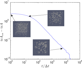
Figure 1: Log-log plot of $\mathrm{tr}\mathbf{A}_{ss}-\mathrm{tr}\mathbf{A}$ vs time shows power-law nature of $\mathrm{tr}\mathbf{A}$ to steady state. Inset images show a typical particle configure at a given point on the curve.

Form of evolution coefficients: Motivated by the power-law decay of $\mathrm{tr}\mathbf{A}$ to steady state we have just determined, we choose the following functional forms for the $c_{i}$ coefficients:

$$c_{1} =\frac{1}{3}\left(\frac{Z_{0}}{\tau}\left(Z_{0}-\mathrm{tr}\mathbf{A}\right)^{n}+\beta Z_{\infty}\left|\mathbf{D}\right|\right)$$ (10)

$$c_{2} =-\left(\frac{1}{\tau}\left(Z_{0}-\mathrm{tr}\mathbf{A}\right)^{n}+\beta\left|\mathbf{D}\right|\right)$$ (11)

$$c_{3} =\alpha$$ (12)

where $Z_{0}=\mathrm{tr}\mathbf{A}_{ss}$ (in the absence of flow), $Z_{\infty}=\mathrm{tr}\mathbf{A}_{ss}$ as $\left|\mathbf{D}\right|\rightarrow\infty$, $\tau$ is the time scale of thermal fabric relaxation, $\beta$ reflects the network creation or disruption due to non-affine flow perturbations, $\alpha$ is the initial rate of anisotropy formation when started from an isotropic state, and $n$ characterizes the relaxation to the no-flow steady state (see Fig 1). The above constraints imply the following inequalities on these parameters: $Z_{0},Z_{\infty}>2$; $\tau,\beta>0>\sqrt{2/3}\,\alpha>-\beta Z_{\infty}/3$. The value of $n$ can be predicted from the discrete simulation data by taking the trace of Eq (4), setting $\mathbf{L}$ to $\mathbf{0}$, integrating to find $\mathrm{tr}\mathbf{A}$ as a function of time, and relating the answer back to the power-law in Eq 9. Using this, we find $n=1.34$.

Experimental Methods: The system studied is a carbon black suspension prepared in the absense of dispersant by mixing carbon black particles in a light mineral oil. Details of materials and preparation can be found in the supplementary material. Simultaneous rheo-electric measurements were performed using a custom device, described in more detail in the supplementary material. A schematic of the device used to perform the rheo-electric measurements is shown in Fig 2.

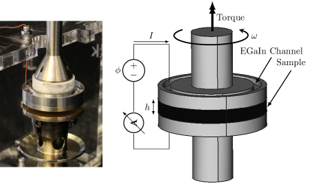
Figure 2: Device used to perform rheo-electric measurements.

Two sets of experiments were performed using the setup described above. The first was a set of steady-state current measurements taken at nominal shear rates in the range $\dot{\Gamma}=\omega R/h\in\left[0,300\right]s^{-1}$. At each shear rate, both the current and stress were allowed to equilibrate before the measurement was recorded to ensure that it had relaxed to its steady value. The shear rates were swept in descending order to mitigate complications such as shear-induced phase separation that arise at low shear rates, below $\dot{\Gamma}\sim 20s^{-1}$ Helal et al. (tion).

The second dataset was a collection of transient ramp tests wherein current data was collected continuously for the duration of the test. The ramp tests consisted of 5 minutes of nominal shear rate $\dot{\Gamma}=\dot{\Gamma}_{1}$, ramping linearly to $\dot{\Gamma}_{2}$ over duration $t_{R}$, holding for 5 minutes, and abruptly setting $\dot{\Gamma}=0$, collecting data for 15 additional minutes. Pre-shear at $\dot{\Gamma}=100s^{-1}$ was applied for 5 minutes before each test to ensure consistent initial conditions.

The parameters $Z_{0}$, $Z_{\infty}$, $\beta$, and $\alpha$ were fitted to the steady-state current measurements using the $\mathtt{fminunc}$ Matlab optimization routine, minimizing the squared difference between predicted and measured electrical currents. The $\tau$ parameter, which is primarily responsible for controlling the fabric’s relaxation time, was chosen from the experimental dynamics of the ramp tests. Lastly, the $k_{1}$ parameter can be chosen to match the steady-state current observed at $\dot{\Gamma}=0$.

The predicted current is calculated by evaluating the integral

$$I(t)=2\pi\int_{0}^{R}K_{zz}(\mathbf{A}(r,t))\cdot\frac{\phi}{h}r\,dr$$ (13)

where $K_{zz}$ is the component of conductivity perpendicular to the plate, $\phi$ is the applied potential difference across the plates, $h$ is the plate separation, and $R$ is the plate radius. Note that the fabric tensor is a function of radial position; each point along a radius is subjected to a different shear rate due to the applied torsional motion, and thus evolves differently.

The form of (13) can be modified slightly in order to solve for the current at steady-state for a given nominal shear rate $\dot{\Gamma}$, by substituting $\mathbf{A}(r,t)$ with $\mathbf{A}_{ss}(\dot{\gamma}=\dot{\Gamma}r/R)$ where $\mathbf{A}_{ss}(\dot{\gamma})$ is the steady-state fabric tensor, whose components are obtained algebraically from Eq 4 by defining $\mathbf{D}$ and $\mathbf{W}$ to correspond to simple shearing at $\dot{\gamma}$ and setting $\dot{\mathbf{A}}=\mathbf{0}$. A detailed outline of the fitting procedure can be found in the supplementary material.

To simulate the electrical current for a transient test, the evolution law must be directly integrated at each point across the disk where the conductivity will be evaluated. To do this, one must input the time-dependent nominal shear-rate $\dot{\Gamma}(t)$ from the experimental protocol. The evolution law was numerically integrated using the 4th-order Runge-Kutta method implemented in the Matlab function $\mathtt{ode45}$. After the fabric is known for all time at each point, (13) can be approximated directly using a Riemann sum to give the predicted current as a function of time.

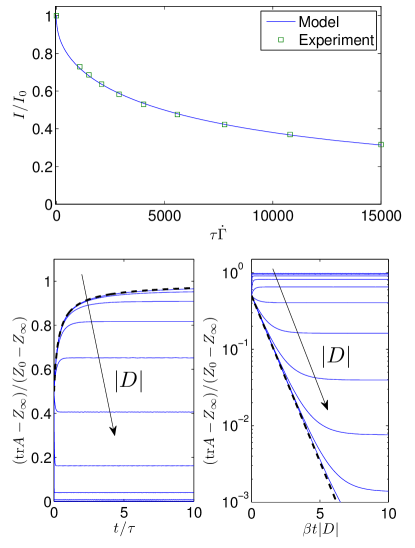
Figure 3: Top: Model fit of steady-state current measurements at different nominal shear rates. Values are normalized by static current measurement $I_{0}$. Bottom: Evolution of $Z=\mathrm{tr}\mathbf{A}$ in pure shearing under different shear rates, as predicted by the model. (Left) Small $\left|\mathbf{D}\right|$ yields power-law approach of $Z$ to steady state; $|Z-Z_{0}|\sim t^{-1/n}$ as $|D|\to 0$, dotted line. (Right) Large $\left|\mathbf{D}\right|$ yields exponential approach to steady state; $\log(Z-Z_{\infty})\sim-\left|\mathbf{D}\right|t$ as $|D|\to\infty$, dotted line.

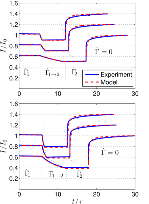
Figure 4: Transient ramp experiments from (top) $\tau\dot{\Gamma}_{1}=2500$ to $\tau\dot{\Gamma}_{2}=5000$, and (bottom) $\tau\dot{\Gamma}_{1}=2500$ to $\tau\dot{\Gamma}_{2}=10000$ with ramp times $t_{R}/\tau$ of 0.6, 1.2, and 6 (top to bottom). A vertical offset of 0.2 has been added between successive curves for clarity, with the y-axis correct as displayed for the bottom curve. Current values are normalized by the static current measurement $I_{0}$.

Results: The power law index $n$ was determined a priori using the discrete simulation, and all others were found using the fitting procedure described above. The parameters used to generate all of the following plots, which satisfy all necessary constraints, are $Z_{0}=7$, $Z_{\infty}=2.41$, $\tau=50\,s$, $\beta=0.009$, $\alpha=-0.0089$, $n=1.34$, and $k_{1}=0.0282\;S/m$.

The top of Fig 3 shows the steady-state current predicted by the model compared to experimental data at various shear rates. The results indicate the model does an excellent job predicting the steady-state current measurements over the entire tested range of $\dot{\Gamma}$. The bottom of Fig 3 demonstrates the behavior of the model regarding evolution of the coordination number from a common starting value for various scalar strain-rates, $\left|\mathbf{D}\right|$, in pure shearing (same data is shown in both plots, but under different axes definitions). Dotted lines show analytical solutions in the limiting cases of $\left|\mathbf{D}\right|\rightarrow 0$ and $\left|\mathbf{D}\right|\rightarrow\infty$ respectively. The model’s prediction that $Z$ exponentially decays to its steady state in the shear-dominated ($|\mathbf{D}|\gg(\beta\tau)^{-1}$) limit agrees with previous simulations of attractive fluid-particle systems Martys et al. (2009).

The results in Fig 4 show the temporal evolution of the current under imposed shearing normalized by the static current measurement. The close agreement indicates that the model is capable of making accurate, quantitative predictions for the transient behavior of the normalized current. The model and the data match closely over the majority of the experiment, and the model reproduces the final relaxation behavior correctly.

Discussion: We have demonstrated a model for the conductivity of sheared suspensions, by linking conductivity and flow to a common microstructural description. Although the model parameters were obtained using conductivity measurements, it is interesting to note the following points, which emphasize that the structure indeed plays the assumed role: (i) the best-fit parameters obtained from the calibration experiment obey constraints implied by a particle structure (5-8), (ii) the parameters predict a reasonable static coordination number for a particle system, and (iii) the structural evolution model, on which the experimental agreement hinges, gives the same asymptotic behaviors as those observed in suspension simulations. Conversely, our approach highlights the possibility of using conductivity measurements to infer discrete microstructural properties of systems, a notion also suggested in Zhuang et al. (1995). It should be noted that a simpler constitutive specialization of the $c_{i}$ functions using $n=0$ does not not capture the measured evolution of conductivity well. A model using $n=0$ predicts exponential, rather than power-law, relaxation of fabric upon cessation of flow. The resulting conductivity evolution cannot predict the observed behavior shown in Fig 4. The new model (2, 4, 10-12) can be applied as a quantitative tool for designing systems of flowing, electrically-active pariculate suspensions, for example in a semi-solid flow battery architecture Duduta et al. (2011); Helal et al. (2014); Smith et al. (2014). Because the shear-induced conductivity loss can be strong even under moderate shear rates, the ability to predict this component of the performance envelope through a quantitative continuum model should enable subsequent geometric and flow protocol optimization.

Acknowledgements: The authors acknowledge support from the Joint Center for Energy Storage Research (JCESR), an Energy Innovation Hub funded by the U.S. Department of Energy, Office of Science, Basic Energy Science (BES). The authors declare that there are no conflicts of interest.

References

- Bischoff et al. (2002) J. E. Bischoff, E. M. Arruda, and K. Grosh, Journal of Applied Mechanics 69, 570 (2002).
- Deneweth et al. (2013) J. M. Deneweth, S. G. McLean, and E. M. Arruda, Journal of biomechanics 46, 1604 (2013).
- Frederick and Armstrong (2007) C. O. Frederick and P. Armstrong, Materials at High Temperatures 24, 1 (2007).
- Azéma et al. (2012) E. Azéma, N. Estrada, and F. Radjai, Physical Review E 86, 041301 (2012).
- da Cruz et al. (2005) F. da Cruz, S. Emam, M. Prochnow, J.-N. Roux, and F. Chevoir, Physical Review E 72, 021309 (2005).
- Mehrabadi et al. (1982) M. M. Mehrabadi, S. Nemat-Nasser, and M. Oda, International Journal for Numerical and Analytical Methods in Geomechanics 6, 95 (1982).
- Oda et al. (1982) M. Oda, S. Nemat-Nasser, and M. M. Mehrabadi, International Journal for Numerical and Analytical Methods in Geomechanics 6, 77 (1982).
- Radjai et al. (2012) F. Radjai, J.-Y. Delenne, E. Azéma, and S. Roux, Granular Matter 14, 259 (2012).
- Satake (1978) M. Satake, Continuum Mechanical and Statistical Approaches in the Mechanics of Granular Materials , 47 (1978).
- Sun and Sundaresan (2011) J. Sun and S. Sundaresan, Journal of Fluid Mechanics 682, 590 (2011).
- Stephen and Straley (1974) M. J. Stephen and J. P. Straley, Reviews of Modern Physics 46, 617 (1974).
- Grenard et al. (2011) V. Grenard, N. Taberlet, and S. Manneville, Soft Matter 7, 3920 (2011).
- Grenard et al. (2014) V. Grenard, T. Divoux, N. Taberlet, and S. Manneville, Soft Matter 10, 1555 (2014).
- Koumakis et al. (2012) N. Koumakis, M. Laurati, S. U. Egelhaaf, J. F. Brady, and G. Petekidis, Physical Review Letters 108, 098303 (2012).
- Mohraz and Solomon (2005) A. Mohraz and M. J. Solomon, Journal of Rheology 49, 657 (2005).
- Negi and Osuji (2009) A. S. Negi and C. O. Osuji, Rheologica Acta 48, 871 (2009).
- Osuji et al. (2008) C. O. Osuji, C. Kim, and D. A. Weitz, Physical Review E - Statistical, Nonlinear, and Soft Matter Physics 77, 8 (2008).
- Osuji and Weitz (2008) C. O. Osuji and D. A. Weitz, Soft Matter 4, 1388 (2008).
- Park and Ahn (2013) J. D. Park and K. H. Ahn, Soft Matter 9, 11650 (2013).
- Santos et al. (2013) P. H. S. Santos, O. H. Campanella, and M. A. Carignano, Soft Matter 9, 709 (2013), arXiv:1307.3615 .
- Trappe et al. (2001) V. Trappe, V. Prasad, L. Cipelletti, P. N. Segre, and D. A. Weitz, Nature 411, 772 (2001).
- Trappe and Weitz (2000) V. Trappe and D. A. Weitz, Physical Review Letters 85, 449 (2000).
- Duduta et al. (2011) M. Duduta, B. Ho, V. C. Wood, P. Limthongkul, V. E. Brunini, W. C. Carter, and Y.-M. Chiang, Advanced Energy Materials 1, 511 (2011).
- Youssry et al. (2013) M. Youssry, L. Madec, P. Soudan, M. Cerbelaud, D. Guyomard, and B. Lestriez, Physical Chemistry Chemical Physics 15, 14476 (2013).
- Alig et al. (2007) I. Alig, T. Skipa, M. Engel, D. Lellinger, S. Pegel, and P. Pötschke, Physica Status Solidi (B) 244, 4223 (2007).
- Amari and Watanabe (1990) T. Amari and K. Watanabe, Journal of Rheology 34, 207 (1990).
- Bauhofer et al. (2010) W. Bauhofer, S. Schulz, A. E. Eken, T. Skipa, D. Lellinger, I. Alig, E. Tozzi, and D. Klingenberg, Polymer 51, 5024 (2010).
- Schulz and Bauhofer (2010) S. Schulz and W. Bauhofer, Polymer 51, 5500 (2010).
- Smith et al. (2014) K. C. Smith, Y.-M. Chiang, and W. Craig Carter, Journal of the Electrochemical Society 161, A486 (2014).
- Hoekstra et al. (2003) H. Hoekstra, J. Vermant, J. Mewis, and G. G. Fuller, Langmuir , 9134 (2003).
- Morris and Katyal (2002) J. F. Morris and B. Katyal, Physics of Fluids 14, 1920 (2002).
- Vermant and Solomon (2005) J. Vermant and M. J. Solomon, Journal of Physics: Condensed Matter 17, R187 (2005).
- Olsen and Kamrin (2015) T. Olsen and K. Kamrin, Soft Matter 11, 3875 (2015).
- Hand (1962) G. L. Hand, Journal of Fluid Mechanics 13, 33 (1962).
- Rivlin (1955) R. S. Rivlin, Journal of Rational Mechanics and Analysis 4, 681 (1955).
- Marsden and Hughes (1994) J. E. Marsden and T. J. Hughes, Mathematical foundations of elasticity (Courier Corporation, 1994).
- Gurtin et al. (2010) M. E. Gurtin, E. Fried, and L. Anand, The Mechanics and Thermodynamics of Continua (Cambridge University Press, 2010).
- Jr and Sander (1981) T. W. Jr and L. Sander, Physical Review Letters 47 (1981).
- Happel and Brenner (2012) J. Happel and H. Brenner, Low Reynolds number hydrodynamics: with special applications to particulate media, Vol. 1 (Springer Science & Business Media, 2012).
- Helal et al. (tion) A. Helal, T. Divoux, X. Chen, Y.-M. Chiang, and G. H. McKinley, Phys. Rev. Applied (InPreparation).
- Martys et al. (2009) N. S. Martys, D. Lootens, W. George, and P. Hébraud, Physical Review E 80, 031401 (2009).
- Zhuang et al. (1995) X. Zhuang, A. Didwania, and J. Goddard, Journal of Computational physics 121, 331 (1995).
- Helal et al. (2014) A. Helal, K. Smith, F. Fan, X. W. Chen, J. M. Nobrega, Y.-M. Chiang, and G. H. McKinley, “Study of the rheology and wall slip of carbon black suspensions for semi-solid flow batteries,” The Society of Rheology 86th Annual Meeting (2014).