THE INNER EDGE OF THE HABITABLE ZONE FOR SYNCHRONOUSLY ROTATING PLANETS AROUND LOW-MASS STARS USING GENERAL CIRCULATION MODELS

Abstract

Terrestrial planets at the inner edge of the habitable zone of late-K and M-dwarf stars are expected to be in synchronous rotation, as a consequence of strong tidal interactions with their host stars. Previous global climate model (GCM) studies have shown that, for slowly-rotating planets, strong convection at the substellar point can create optically thick water clouds, increasing the planetary albedo, and thus stabilizing the climate against a thermal runaway. However these studies did not use self-consistent orbital/rotational periods for synchronously rotating planets placed at different distances from the host star. Here we provide new estimates of the inner edge of the habitable zone for synchronously rotating terrestrial planets around late-K and M-dwarf stars using a 3-D Earth-analog GCM with self-consistent relationships between stellar metallicity, stellar effective temperature, and the planetary orbital/rotational period. We find that both atmospheric dynamics and the efficacy of the substellar cloud deck are sensitive to the precise rotation rate of the planet. Around mid-to-late M-dwarf stars with low metallicity, planetary rotation rates at the inner edge of the HZ become faster, and the inner edge of the habitable zone is farther away from the host stars than in previous GCM studies. For an Earth-sized planet, the dynamical regime of the substellar clouds begins to transition as the rotation rate approaches $\sim 10$ days. These faster rotation rates produce stronger zonal winds that encircle the planet and smear the substellar clouds around it, lowering the planetary albedo, and causing the onset of the water-vapor greenhouse climatic instability to occur at up to $\sim 25\%$ lower incident stellar fluxes than found in previous GCM studies. For mid-to-late M-dwarf stars with high metallicity and for mid-K to early-M stars, we agree with previous studies.

1 Introduction

The study of habitable zones (HZs) has received increased attention with the discoveries of terrestrial mass/size planets from both ground-based surveys and from the Kepler mission (Kasting et al., 1993; Selsis et al., 2007b; Kopparapu et al., 2013; Leconte et al., 2013; Yang et al., 2013; Kopparapu et al., 2014; Wolf & Toon, 2014; Yang et al., 2014a; Wolf & Toon, 2015). Specifically, terrestrial planets in the HZs of M-dwarf stars have received the most recent scrutiny because their shorter orbital periods increase their chances of detection compared to planets around G stars. M-dwarfs are the most numerous stars in the Galaxy and are also our closest neighbors. The upcoming James Webb Space Telescope (JWST) mission, with targets provided by the ongoing K2 mission and planned Transiting Exoplanet Survey Satellite (TESS, Ricker et al. (2014)), may be capable of probing the atmospheric composition of terrestrial planets around a nearby M-dwarf. This will be our first opportunity to obtain spectral information on terrestrial planets in the habitable zones of M-dwarf stars. The initial targets for these missions will likely be planets near the inner edge of the HZ, precisely because such planets have an increased probability of transit and are more likely to get their masses estimated by RV techniques. Recent work (Boyajian et al. 2012, Boyajian et al. 2014, Terrien et al. 2015, Mann et al. 2015, Newton et al. 2015) has resulted in better stellar characterization and more accurate temperatures and radii for the M dwarfs. Thus, determining an accurate inner edge of the HZ around late-K and M-dwarf stars will soon become crucial for interpreting the data from these missions.

Previous 1-D climate model studies of HZs (Kasting et al., 1993; Selsis et al., 2007b; Kopparapu et al., 2013, 2014) predicted that, for a water-rich planet such as Earth, two types of habitability limits exist near the inner edge: (1) A moist greenhouse limit, which occurs when the stratospheric water vapor volume mixing ratio becomes $>10^{-3}$, causing the planet to lose water by photolysis and subsequent loss of hydrogen to space; (2) A runaway greenhouse limit, whereby the outgoing thermal-infrared radiation from the planet reaches an upper limit beyond which the surface temperature increases uncontrollably, causing the oceans to evaporate. Habitable climates may be terminated via the moist greenhouse process long before a thermal runaway occurs. Widespread surface habitability for human life could be terminated by rising temperatures well before even a moist greenhouse is reached, because of limits on biological functioning (Sherwood & Huber, 2010).

1-D climate models that are being used currently have significant limitations. In particular, it is hard to accurately model planets within the HZs of late-K and all M-dwarf stars because such planets are expected to be tidally locked. If the planet’s orbital eccentricity is near zero, this can result in synchronous rotation, in which one side of the planet always faces the star. Indeed, a recent study by Leconte et al. (2015) argued that all planets near the inner edge of the HZ of M-dwarfs (masses $<0.6$ M_⊙; Dotter et al. (2008)) should rotate synchronously. Somewhat surprisingly, according to Leconte et al. (2015), planets orbiting in the outer HZs of M and K-dwarf stars should not rotate synchronously because their rotation rates are perturbed by thermal tides.

Recently, Yang et al. (2013, 2014a) used the Community Atmosphere Model (CAM) from the National Center of Atmospheric Research, Boulder CO, to simulate an Earth-size water-rich planet in various spin-orbit configurations. Not surprisingly, they found that atmospheric circulation, and thus the predominant location of clouds, is critically influenced by the Coriolis force (which results from the planetary rotation rate). Rapidly rotating planets, like Earth, have latitudinally banded circulation patterns. However, for slowly rotating planets the Coriolis force is too weak to form such banded structures. Instead, strong and persistent convection occurs at the substellar region, creating a stationary and optically thick cloud deck. This causes a strong increase in the planetary albedo, cooling the planet, and stabilizing climate against a thermal runaway for large incident stellar fluxes. This result was found to be qualitatively robust for a wide variety of model configurations and parameter sensitivity tests. It has also been qualitatively corroborated by a generalized version of the NASA GISS GCM (Way et al., 2015). Thus, it initially appears that the substellar convection and cloud mechanisms on slow rotators is a robust prediction of climate models. This moves the inner edge of the habitable zone significantly closer to the star, reaching almost twice the stellar flux predicted by 1-D models (Kopparapu et al., 2013, 2014).

A caveat should be added to the above conclusion, however. In doing their calculations, Yang et al. (2014a) assumed a constant orbital period of 60 days at the inner edge of the HZ for synchronously rotating planets around M and K-dwarf stars. While this assumption is sufficient to demonstrate the concept of cloud stabilization, it is not consistent with Kepler’s third law. Moreover, the climatic differentiation between “rapid” and “slow” rotators is not a binary choice, but rather is a continuous function of changing Coriolis force (Yang et al., 2014a). Thus, correcting the orbital/rotational period for synchronously rotating planets around M and K-dwarfs may indeed change our view of the inner edge of the HZ.

Whether atmospheric circulation of one planet is in the rapidly rotating or slowly rotating regime mainly depends on the ratio of Rossby deformation radius to the planetary radius (Edson et al. 2011; Showman et al. 2013; Carone2014). If the ratio is larger than one, the planet will be in the slow rotating regime, and if the ratio is smaller than one, the planet will be in the rapidly rotating regime. For the synchronously rotating planets we disussed here, the transition from the slowly rotating regime to the rapidly rotating regime occurs when the planetary rotation period is approximately 5 days for planets with $1$ R_⊕ and approximately 10 days for planets with 2 R_⊕, as pointed out by Yang et al. (2013). Different planets in one of the two regimes will have very similar patterns of atmospheric circulation and surface climate.

For synchronously rotating planets, the orbital period and the rotational period are by definition in 1:1 resonance. For example, Gl 667Cc (Anglada-Escude et al., 2013), a super-Earth around an M-dwarf star with effective temperature $T_{eff}=3350$K, has an orbital period of $28.1$ days (Robertson et al., 2014). This planet receives a stellar flux of $0.87$ times Earth’s flux. The model planets at the inner edge of the HZ with a $60$ day orbital period considered by Yang et al. (2014a) would need to be at roughly twice the observed period of Gl 667Cc to be consistent with Kepler’s third law. Therefore, they should be receiving roughly $\sim 0.3$ Earth’s flux, which puts those model planets beyond the outer edge of the HZ, rather than at the inner HZ limit. Planets at the inner edge of the HZ of M-dwarfs have shorter orbital periods than planets around G-dwarfs. Since such planets are synchronously rotating, shorter orbital periods mean shorter rotational periods. As Yang et al. (2014a) pointed out, a rapidly rotating planet tends to have decreased substellar cloud cover, lowering its albedo, and hence moving the inner edge of the HZ further away from the star. Our goal in this paper is to use self-consistent orbital and rotational periods for planets and to derive new inner HZ limits for synchronously rotating planets around M and late-K dwarfs.

The outline of the paper is as follows: In §2 we briefly describe our general circulation model. In §3 we present results from our model, comparing to previous studies, and present new HZ limits. We conclude in §4.

2 Model

We used the Community Atmosphere Model v.4 (CAM4) developed by the National Center for Atmospheric Research (NCAR). For an in-depth technical description of CAM4, see Neale et al. (2010). We configured the model to simulate an Earth-size aquaplanet (i.e. globally ocean covered) in synchronous rotation (1:1 spin-orbit resonance) around M and late-K dwarfs. We ran the model at a horizontal resolution of $1.9^{\circ}\times 2.5^{\circ}$ with $26$ vertical levels. The assumed atmosphere consists of 1 bar of N₂, 1 ppm of $\rm{CO_{2}}$ and no $\rm{CH_{4}}$, O₂, O₃, trace gases, or aerosols. We used a thermodynamic (slab) ocean model with a uniform depth of 50 m (a standard value for slab ocean models) and zero ocean heat transport. The ocean surface albedo is $0.06$ in the visible and 0.07 in the near-IR. We assumed zero obliquity and zero eccentricity, consistent with the assumption of synchronous rotation; thus, there is no seasonal cycle. Stellar spectra are assumed to be blackbody to facilitate comparison with Yang et al. (2014a). We use a model time step of 1800 seconds. Sub-grid-scale cloud parameters were taken as the default values for our given resolution and dynamical core selections. Following a methodology similar to that of Yang et al. (2014), we moved planets closer to the star (by increasing the stellar flux) until the the model becomes unstable. We used the last converged solution as a proxy for the inner edge of the HZ.

3 Results

3.1 Calculation of Correct Orbital Periods

Following Kepler’s third law, the orbital period $P$ is a function of orbital semi-major axis $a$ and the stellar mass $M_{\star}$:

$$P\mathrm{(years)} = \left[\frac{a\mathrm{(AU)}^{3}}{M_{\star}/M_{\odot}}\right]^{1/2}$$ (1)

The stellar flux incident on a planet, $F_{P}$, compared to the flux on Earth ($F_{\oplus}$) can be written as:

$$F_{P}/F_{\oplus} = \frac{L_{\star}/L_{\odot}}{a^{2}}$$ (2)

where $L_{\star}/L_{\odot}$ is the luminosity of the star with respect to the bolometric luminosity of the Sun. Combining these two equations, the orbital period can be written as:

$$P(years) = \left[\left(\frac{L_{\star}/L_{\odot}}{F_{P}/F_{\oplus}}\right)^{3/4}\right]\left[{M_{\star}/M_{\odot}}\right]^{-1/2}$$ (3)

This equation indicates that the orbital period of a planet in synchronous rotation can be calculated from the luminosity, mass and the incident flux, and it cannot be chosen irrespective of the stellar type. This result is obvious, and not new, but it has significant implications for where the inner edge of the HZ is located. Moreover, for a star with a fixed effective radiating temperature, $T_{eff}$, stellar luminosity depends on the metallicity of a star (Chabrier & Baraffe, 2000; Dotter et al., 2008, see Fig. 2a) because of changes in the opacity of the stellar atmosphere. So the HZ also varies as a function of stellar metallicity (Young et al., 2012). In this srudy, we used the Dartmouth stellar evolution database (Dotter et al., 2008) to obtain $L_{\star}$ and $M_{\star}$ for both low ($[Fe/H]=-0.5$) and high ($[Fe/H]=0.3$) metallicities, as a function of $T_{eff}$. For convenience, we parameterized the relationship between $T_{eff}$, $M_{\star}$, and $L_{\star}$ and provided the coefficients in Table 3.1:

$$y = a+bx+cx^{2}+dx^{3}+ex^{4}+fx^{5}$$ (4)

Here, $y$ can be either $M_{\star}/M_{\odot}$ or $L_{\star}/L_{\odot}$, and $x$ is $T_{eff}$. These relations apply only for stars with $3300\leq T_{eff}\leq 4500$K, as we are focused on low-mass stars which may have synchronously rotating planets near the inner edge of their HZs. The lower limit of $3300$K is based on the completeness of the Dartmouth model grid for our chosen parameters.

[h!] Coefficients to be used in Eq.(4) to calculate stellar luminosity and mass from $T_{eff}$. [Fe/H] $y$ $a$ $b$ $c$ $d$ $e$ $f$ $L_{\star}/L_{\odot}$ $-48.048$ $0.0645$ $-3.442\mathrm{E}-5$ $9.098\mathrm{E}-9$ $-1.192\mathrm{E}-12$ $6.209\mathrm{E}-17$ $-0.5$ $M_{\star}/M_{\odot}$ $874.787$ $-1.121$ $5.709\mathrm{E}-4$ $-1.445\mathrm{E}-7$ $1.821\mathrm{E}-11$ $-9.138\mathrm{E}-16$ $L_{\star}/L_{\odot}$ $-27.044$ $0.033$ $-1.640\mathrm{E}-5$ $4.036\mathrm{E}-9$ $-4.961\mathrm{E}-13$ $2.452\mathrm{E}-17$ $0.3$ $M_{\star}/M_{\odot}$ $-406.344$ $0.480$ $-2.268\mathrm{E}-4$ $5.342\mathrm{E}-8$ $-6.271\mathrm{E}-12$ $2.935\mathrm{E}-16$

One can calculate a range of orbital periods using Eq.(3), substituting the values for $M_{\star}/M_{\odot}$ and $L_{\star}/L_{\odot}$ obtained from Eq.(4), assuming a given $F_{P}/F_{\oplus}$.

For a $3400$K star, using Eq.(4), the corresponding stellar luminosity and mass are $0.0049L_{\odot}$ and $0.189M_{\odot}$, respectively, for the low-metallicity case, $0.0204L_{\odot}$ and $0.416M_{\odot}$ for the high-metallicity case. A high metallicity star has a higher mean atmospheric opacity, so for a certain stellar mass and age, a given optical depth is higher in the atmosphere and therefore at a lower temperature (lower Teff). To match the same Teff as a lower metallicity star (as is done here), the higher metallicity star (at a given age) must be more massive, increasing the overall stellar energy output and therefore Teff. If one assumes $P=60$ days in Eq.(3), the corresponding stellar fluxes are $0.165F_{\oplus}$ for $[Fe/H]=-0.5$, and $0.406F_{\oplus}$ for $[Fe/H]=0.3$. These fluxes are much lower than the value used by Yang et al. (2014a) at the inner HZ; indeed, they are substantially lower than that of present day Earth. Thus, a planet with $P=60$ days around a $T_{eff}=3400$K is more likely to have a frozen surface than to be at the precipice of a runaway.

One can calculate a consistent orbital period from Eq.(3), assuming an inner HZ flux of $1.626F_{\oplus}$ calculated from Yang et al. (2014a) for a $3400$K star. Then, the orbital period that the planet should have is $10.79$ days for $[Fe/H]=-0.5$, and $21.21$ days for $[Fe/H]=0.3$, both much shorter than the $60$-day period assumed by Yang et al. (2014a). We performed simulations at both of these orbital periods. For the $10.79$-day period, the planet warms rapidly and no converged solution is found. By contrast, the $21.2$-day case and the (unphysical) $60$-day case remain climatologically stable (Fig.1). Both the 21.2-day and 60-day simulations exhibit similar climatological characteristics, with planetary albedos of $0.54$ and mean surface temperatures in the upper end of 270 K. While the $10.79$-day case is not quite a “fast” rotator like Earth, the increased rotation rate alters dynamics such that some of the substellar cloud deck is advected to the anti-stellar side of the planet, lowering the planetary albedo, and causing the planet to become much warmer than in the slowly rotating cases.

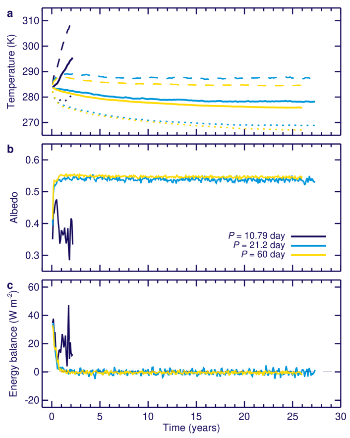
Figure 1: Time series data from three simulations: $[Fe/H]=-0.5$ ($P=10.79$ day), $[Fe/H]=0.3$ ($P=21.2$ day), and $P=60$ day period. Each simulation is irradiated by $2211$ W m^-2 of solar radiation. This value is the inner edge flux for a star with $T_{eff}=3400$K, as calculated by Yang et al. (2014a) for their slowly rotating case. Panel a shows the temporal evolution of the surface temperature, panel b shows the planetary albedo, and panel c shows the top-of-atmosphere energy balance (net solar in minus net longwave out). In all figures solid curves show the global mean quantity. Dashed and dotted curves in panel a show the dayside and nightside mean temperatures, respectively.

For slower rotation rates ($P>20$ days), thick substellar clouds produce a large planetary albedo, which stabilizes the climate against strong solar radiation. However, as $P$ approaches $\sim 10$ days, the sub-stellar cloud decks begins to be smeared around the planet, resulting in a reduced albedo on the substellar hemisphere, and thus rapidly rising temperatures. The simulation with $P=10.79$ days experiences numerical instability after only a few years, with a residual energy imbalance of $>10$ Wm^-2. While stable climates may lie beyond the numerical limits of our model, such atmospheres surely are excessively hot.

One can derive a range of orbital periods that is self-consistent with incident flux (Eq.(3)), using the luminosities and masses from Table 3.1 for different [Fe/H]. Fig.2 shows the correct orbital periods calculated using Eq.(3) that one should use, if one assumes an inner HZ flux $F_{P}/F_{\oplus}$ from the slow-rotator equation of Yang et al. (2014a) for different stars. Also shown are the $P=60$ day periods assumed by Yang et al. (2014a) (blue filled circles), and the results from our own simulations for a $T_{eff}=3400$K star using the correct orbital periods ($10.8$ and $21.2$ days, blue cross and square, respectively) from Eq.(3) to illustrate the differences. The unstable $10.8$-day and the stable $21.2$-day solutions indicate that, for this $T_{eff}=3400$K, the correct inner HZ limit should lie somewhere in between these two orbital periods.

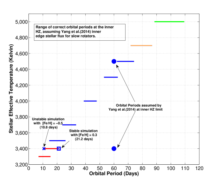
Figure 2: Range of correct orbital periods, $P$, near the inner edge of the HZ for various stars (color horizontal lines), calculated using Eq.(3), assuming an inner HZ flux for slow rotators from Yang et al. (2014a) for both high ([Fe/H] $=0.3$) and low ([Fe/H] $=-0.5$) metallicity cases. Also shown are the $P=60$ day periods (blue filled circles) assumed by Yang et al. (2014a) at the inner edge of the HZ, which are inconsistent with Kepler’s third law. Planets at the inner HZ limit are in 1:1 spin-orbit resonance. Using correct orbital/rotational periods for a $T_{eff}=3400$K star, we find that the inner HZ flux from Yang et al. (2014a) warms a planet beyond the stability limit of our 3-D model (blue cross), around a low [Fe/H] star.

To determine an inner HZ limit that is self-consistent with the calculated orbital periods, we followed the procedure described below for each star with $T_{eff}=3300$K, $3700$K, $4000$K, $4500$K. The lower limit of $3300$K pushes across the edge of the Dartmouth model grid in some parameters, so we limit our simulations to values above this $T_{eff}$. We first calculated the appropriate values of $L_{\star}/L_{\odot}$ and $M_{\star}/M_{\odot}$ from Eq.(4) for that $T_{eff}$, and then chose a range of $F_{P}$ (in Wm^-2) to calculate the corresponding orbital periods for these $F_{P}$. Then, we performed climate simulations at these $P$ and $F_{P}$ values using CAM, assuming synchronous rotation, BB spectral energy distribution (SED) from the star, and zero planetary obliquity. We assumed, as did Yang et al. (2014a), that the last converged solution represents the inner edge of the HZ. The SEDs used in our models are given in Table 3.1.

[h!] Blackbody spectral energy distribution of stars that were considered in this study, written in terms of percentage of total flux in CAM wavelength bands. Band $\lambda_{min}$ (micron) $\lambda_{max}$ (micron) $3300$K $\%$ flux $3700$K $\%$ flux $4000$K $\%$ flux $4500$K $\%$ flux 1 0.200 0.245 0.001913 0.009296 0.02462 0.086219 2 0.245 0.265 0.004174 0.01659 0.03865 0.11277 3 0.265 0.275 0.004139 0.01497 0.03286 0.088338 4 0.275 0.285 0.005468 0.01865 0.03948 0.10097 5 0.285 0.295 0.007856 0.02528 0.05164 0.1257 6 0.295 0.305 0.01225 0.03724 0.07343 0.1703 7 0.305 0.350 0.1158 0.3045 0.5495 1.306 8 0.350 0.640 8.3733 12.902 16.913 22.73 9 0.640 0.700 3.7251 4.7689 5.5102 6.1537 10 0.700 5.000 84.87 79.63 75.524 67.853 11 2.630 2.860 2.1099 1.6653 1.4339 1.0786 12 4.160 4.550 0.8054 0.6082 0.5099 0.3701

3.2 Effect of Correct Orbital Periods on Climate

In this section we discuss the large-scale atmospheric dynamics of synchronously rotating planets. We examine simulations with a stellar effective temperature of 3300 K at the correct orbital period of 9-day which is self-consistent with the assumed incident flux, and for the 60d period, which is not self-consistent. As the planets are assumed to be synchronously rotating, such that the orbital period equals the period of rotation for the planet, we focus on the dynamical contribution toward the reduction in cloud cover caused by these differences in rotation rate.

Fig. 3 shows the latitude-longitude contour plots for three simulations of planets around a $T_{eff}=3300$K star, centered on the substellar point. The first column uses a $60$-day rotation period, as used by Yang et al. (2014a), to define the inner edge of the habitable zone for slow rotators. The second and third columns show contour plots for stable simulations using physically consistent orbital period and solar insolation relationships for both high and low stellar metallicity cases, respectively. For each simulation, the incident flux, rotation rate, mean surface temperature and albedo are listed above each column. While the incident stellar flux is different for each case, the resultant global mean surface temperatures are roughly similar. The key difference between each case is the modification of the cloud albedo as a function of rotation rate. Reducing the rotation rate from 60 to 9-days, decreases the top-of-atmosphere (TOA) albedo by $\sim 25\%$.

Vigorous convection occurs over the substellar point in each of the three cases. Column-integrated cloud water and cloud fractions are expectedly large, as substellar convection lofts water into the free troposphere, creating high upper atmosphere relative humidities and thick convective water clouds, much like in Earth’s tropics today. However, the important differences lie in the details. As the rotation rate of the planet increases from 60 to 16.46 to 9-days for high and low metallicity stars, respectively, the beginnings of a dynamical regime change become evident. This dynamical transition has previously been found by other studies for both highly-irradiated and cool planets of different rotation rates (Heng & Vogt, 2011; Carone et al., 2014; Showman et al., 2013a; Kaspi & Showman, 2015). While all cases maintain strong sub-stellar convection, gradually increasing the rotation produces a corresponding increase in the strength of the zonal winds (Fig 4., Fig 5). Stronger upper level zonal winds begin to smear the clouds into a narrow equatorial band that can stretch around the entire planet. The 500 mb relative humidity (and thus water vapor) closely mirrors the distribution of clouds. The areal extent of clouds over the substellar hemisphere is reduced, most noticeably along the western flank of the sub-stellar point. Increased upper level winds advect clouds eastward, away from their formation region above the sub-stellar point. This reduces the overall fractional cloud cover on the sunlit side of the planet, decreasing the TOA albedo, and thereby warming the climate. Thus, with a 9-day rotation rate, it takes $\sim 26\%$ less solar flux to maintain an equal global mean surface temperature compared to the 60-day rotation case.

Note also that cloud fractions remain high ($\sim 100\%$) on the anti-stellar side of the planet, despite there being little to no convective activity, nor cloud water. On the anti-stellar side, the complete absence of solar surface heating, combined with substellar-to-antistellar atmospheric heat redistribution aloft, creates strong inversions, similar in nature to those that occur during the polar night on Earth. Here, a uniform, thin ice fog extends from the surface up to the inversion cap near 800 mb across the entire night side of the planet. Cloud fractions are near unity, but the clouds contain exceedingly little water and interact only very weakly with the thermal emission from the planet.

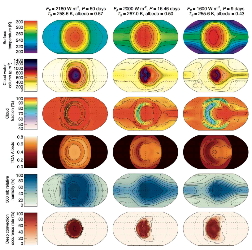
Figure 3: From top to bottom rows: global mean surface temperature, column-integrated cloud water content, column-integrated cloud fraction, top-of-the atmosphere (TOA) albedo, 500 mb relative humidity, and deep convection occurrence rate. These contour maps are shown for three different simulations, each with a different rotation rate around a star with $T_{eff}=3300$K. The first column assumes P = 60 days, following Yang et al. (2014a). The remaining two column figures are the last converged solutions (i.e, planets at the inner HZ limit) for high and low stellar metallicities, whose Ps are calculated self-consistently with the incident flux (FP ) using Eq.(3). These results show that, at least for late M dwarfs, the final converged solution occurs at a lower incident flux, and so the inner HZ limit is not as close as predicted by Yang et al. (2014a). A self-consistent calculation of P yields faster rotating planets, decreasing the substellar clouds and albedo, and thus increasing surface temperature.

Global average temperature and horizontal wind for $T_{eff}=3300$K low metallicity, 9-day and 60-day simulations are shown in Fig 4. Surface temperature and winds are shown in the left column of Fig 4, with inflow along the equator and from the poles into the substellar point at the center. Upper atmosphere temperature and winds at the 200 hPa surface are shown in the right-hand column of Fig 4, with strong zonal westerly flow aloft in the 9-day case and much weaker turbulent flow in the 60-day case. Differences between these cases show up to 4 K of surface warming at the substellar point and more than 10 K along the equator when the rotation rate is increased. Warming of about 4 K also occurs aloft in a gyre near the antistellar point. This warming occurs as a result of a transition from the stabilizing cloud feedback described by Yang et al. (2013) to a banded cloud structure that allows a larger stellar flux incident on the surface. The direction and magnitude of surface winds are similar between the 9-day and 60-day cases, but the pattern of winds aloft differs significantly, with the 9-day case displaying strong upper-level flow that generates a banded cloud structure.

This shift in upper level flow is also apparent in the time-averaged zonal mean zonal wind shown in Fig 5. The 9d case shows strong westerly flow aloft at all latitudes, with two jets prominent at midlatitudes and weaker easterlies along the surface. By comparison, the 60d case shows weaker westerly flow aloft only at tropical latitudes, with easterly jets in the upper atmosphere toward the poles and extremely weak surface winds. This weaker flow in the 60d case provides part of the physical process by which a stabilizing cloud feedback can be maintained; however, the stronger flow when the rotation rate is increased to 9d inhibits the maintenance of this cloud structure.

The mean zonal circulation (MZC) and mean vertical wind for these T3300 (i.e, T${}_{eff}=3300$ K simulations are shown in Fig 6. Rising motion with the MZC and upward vertical wind is apparent at the substellar point, with regions of sinking in the vicinity of the antistellar point. Both of these cases show that the MZC spans the full hemisphere from substellar to antistellar point, which is expected because the orbital periods of all our cases are greater than the critical period $P_{c}$ where a dynamical regime shift would occur (Edson et al. 2011; Carone et al. 2014). The 60-day case shows a stronger zonal circulation than the 9-day case, with greater rising motion at the substellar point and sinking motion at the antistellar point. The symmetry of the MZC and associated rising motion in the 60d case also suggests a symmetric formation for clouds aloft, while the asymmetry observed in the 9d case corresponds to the formation of banded clouds.

The cross-polar circulation is shown in Fig. 7. This circulation pattern is obtained by subtracting the zonal mean from all zonal wind vectors (Joshi1997; Haqq-Misra and Kopparapu 2015), which helps to illustrate the complex three-dimensional patterns that form the general circulation of synchronous rotators. Both cases show flow across the pole at both the 800 hPa and 200 hPa surfaces, although the direction of this flow varies with each experiment. Both cases also display vortices near $0^{\circ}$ to $30^{\circ}$ longitude that contribute to a unique circulation pattern not easily described by the MZC or the mean meridional circulation. This cross-polar circulation is stronger in the 9-day case, both an aloft and along the surface, while the 60d case shows a relatively similar flow pattern but with a reduced magnitude. The increase in cross-polar flow when rotation rate changes from 60d to 9d also provides a mechanism that would disrupt the formation of a stabilizing cloud feedback above the substellar point.

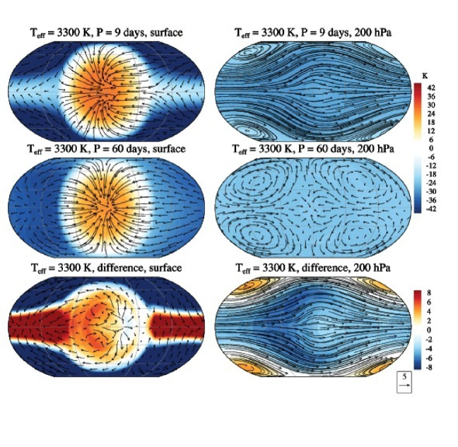
Figure 4: Time average of temperature deviation from the freezing point of water (shading) and horizontal wind (vectors) for T${}_{eff}=3300$ K experiments at the surface (left column) and upper atmosphere (right column). The top row shows the 9d case, the middle row shows the 60d case, and the bottom row shows the difference of the first row minus the second. The substellar point is at the center of each panel.

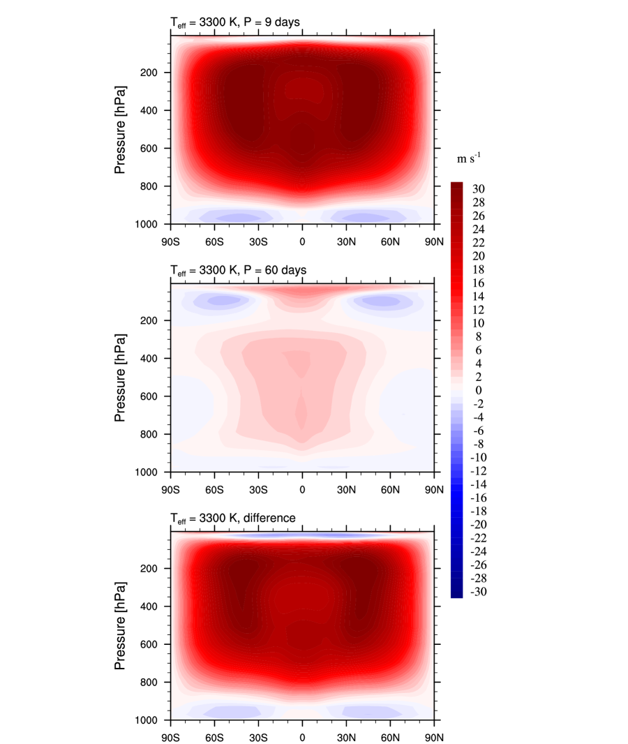
Figure 5: Time average of mean zonal wind (shading) for T${}_{eff}=3300$ K experiments. The top row shows the 9d case, the middle row shows the 60d case, and the bottom row shows the difference of the first row minus the second. The substellar point is centered on the equator at the middle of each panel. Positive (red) shading indicates westerly zonal wind, and negative (blue) shading indicates easterly zonal wind.

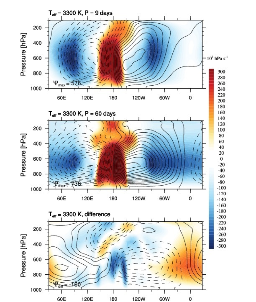
Figure 6: Mean zonal circulation (line contours) and vertical wind (shading) for the T${}_{eff}=3300$ K experiments. The top row shows the 9d case, the middle row shows the 60d case, and the bottom row shows the difference of the first row minus the second. The substellar point is centered on the prime meridian at the middle of each panel. The line contour interval is $30\times 10^{11}$kg s^-1 and the maximum streamfunction $\Psi_{max}$ or difference $\Psi_{diff}$ is shown on each panel in units of $10^{11}$kg s^-1. Solid contours indicate clockwise circulation, and dashed contours indicate anti-clockwise circulation. Positive (orange) shading indicates rising motion, and negative (blue) shading indicates sinking motion.

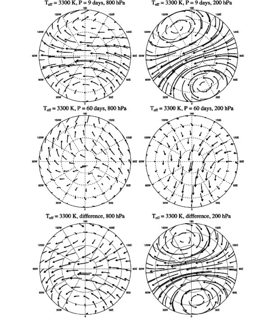
Figure 7: Polar stereographic plots of horizontal wind (vectors) and eddy heat flux (shading) for T${}_{eff}=3300$ K experiments. The top row shows the 9d case, the middle row shows the 60d case, and the bottom row shows the difference of the first row minus the second. The substellar point is centered on the equator and the prime meridian, which is shown at the top of each panel. The plot shows the Northern hemisphere from $30^{\circ}$ to $90^{\circ}$ latitude, and the zonal mean is removed from all zonal wind vectors.

3.3 The Inner HZ Limit with Correct Orbital Periods

Fig. 8 shows our new inner HZ boundary for stars with $3300$K $\leq T_{eff}\leq 4500$K. We show the limits for both low (red) and high (green) [Fe/H] cases. The red curve is farther away from the star because, for a given stellar $T_{eff}$, the low-metallicity star is brighter (see discussion below). For comparison, we also plotted the inner HZ limit from Yang et al. (2014a) (blue) for their 60-day rotator case. These results indicate that the inner edge of the HZ is closer to the star than predicted by Yang et al. (2014a) for $3700$K $\leq T_{eff}\leq 4500$K. This is true for both the high and low [Fe/H] cases, though the difference between these two [Fe/H] is minimal. For stars with $T_{eff}\leq 3700$K, although the low and high [Fe/H] cases diverge dramatically from each other, with the high [Fe/H] case (green) staying closer to the Yang et al. (2014a) inner edge limit (blue). We have also shown several currently confirmed exoplanets on this plot.

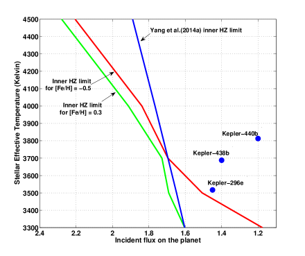
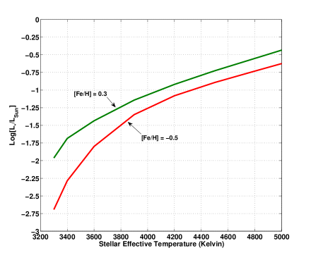
Figure 8: Panel a: Estimates of the inner edge of the HZ for low-mass stars from this study for [Fe/H] $=-0.5$ (red) and $0.3$ (green), compared with Yang et al. (2014a) (blue). Panel b: Dependence of the stellar luminosity on [Fe/H] Dotter et al. (2008). Synchronously rotating planets around lower luminosity stars (red) have faster orbital (and rotational) periods, and hence have a tendency to develop banded cloud formations. This reduces the planetary albedo due to reduction of thick clouds at the substellar point. Therefore, the inner HZ limit is at a lower stellar flux for these low-metallicity, low-luminosity stars.

The reason for this large divergence between the two stellar metallicity cases can be traced to the differences in the stars’ luminosities and planetary rotation rates. Fig. 8 illustrates this point. The difference between $L_{\star}/L_{\odot}$ for [Fe/H] = $0.3$ (blue) and $-0.5$ (red) is largest at lower $T_{eff}$, and that is precisely where we see the divergence in our inner HZ result. The difference in log$[L_{\star}/L_{\odot}]$ for the two metallicities is $\approx 30\%$ at $T_{eff}=3300$K. To receive the same amount of incident $F_{P}$ around a low luminosity star, a planet that is in synchronous rotation needs to be at a shorter $P$ (fast rotator), according to Eq.(3), compared to a high luminosity one. As discussed before, fast rotating planets have stronger Coriolis force, which tends to create more banded cloud formations that reduce the planetary albedo. Furthermore, stars with lower $T_{eff}$ output more flux in the near-infrared (IR) part of the SED. As terrestrial planets at the inner edge of the HZ are expected to have increasing amounts of water vapor in their atmospheres, and as $\rm{H_{2}O}$ is a good near-IR absorber, a small increment in the stellar flux around these low $T_{eff}$ stars would push the planet close to the runaway greenhouse limit. Hence, the inner edge of the HZ is further away around these cool stars.

For stellar effective temperatures greater than 3700 K, we find that the inner edge of the HZ occurs at stellar fluxes up to 20% larger than shown by Yang et al. (2014a). This result was unexpected, as in this regime orbital periods in the HZ remain firmly within the slow-rotating regime, and there is little difference between our model and theirs in the mean state of the climate. In fact, for $T_{eff}=4500$ K, we find self-consistent orbital periods at the inner edge of the HZ of 55.31 and 64.1 days for low- and high-metallicity stars, respectively, bracketing the 60-day value used in Yang et al. (2014a). However, the differences can be traced to subtle differences in the model configuration. Yang et al. (2014a) used CAM3, while here we use CAM4 with an improved numerical algorithm for deep convection. With this patch, CAM4 is able to remain numerically stable at hotter temperatures, while keeping a relatively long model timestep (1800 seconds). To better understand this difference, we repeated simulations for 4500 K stellar effective temperature star using CAM3 without any numerical improvement to the deep convection scheme, but with an exceedingly short model timestep (100 seconds) to improve numerical stability. When we do this, we find similar results to those found with CAM4 using a longer timestep. Thus, there is no actual conflict between the results shown here and those shown in Yang et al. (2014a) for $T_{eff}>3700$K; rather, it is an issue of model configuration and numerical stability. This point highlights why model intercomparisons are of the utmost importance.

3.4 The nature of the last converged solution

Computational and numerical limitations prevent current Earth-derivative 3D climate models from exploring the full runaway greenhouse process, through surface temperatures beyond the critical point and the vaporization of the entire oceans. This has led to the so-called “last converged solution” criteria being used as a proxy for the inner edge of the HZ (Wolf and Toon, 2014; Yang et al. 2014). While at first glance this criteria appears unsatisfying, the last converged solution may nonetheless be diagnostic of an imminent climatic state transition. Using CAM4 to study Earth (a rapid rotator), Wolf and Toon (2014) first found the last converged solution to have a global mean surface temperature of $\sim 313$ K. However, in a subsequent study, using the same model but with improved numerics, Wolf and Toon (2015) showed that their previous assumed last converged solution was actually hovering just below the threshold of an abrupt transition into a hotter climate state.

In Fig. 9, we summarize the global mean climates of our last converged solutions as a function of the stellar effective temperature. There is a definite trend in the global mean surface temperature of the last converged solution, with the last stable temperatures being significantly lower around 3300 K stars compared to 4500 K stars. This trend is caused by the interaction of different spectral energy distributions (SEDs) with atmospheric water vapor. Changes to the top of the atmosphere (TOA) albedo also display a trend, in this case linked most tightly to the rotation rate of the planet due to the dynamical modulation of the cloud fields, as is discussed in section 3.2. SED does affect atmospheric scattering, with planets around bluer stars scattering more of the incident sunlight than those around redder stars; however this effect is relatively small at the atmospheric temperatures and pressures we consider in this study. Here, the TOA albedo is dominated by the clouds rather than by atmospheric scattering. As the rotation rate (Fig. 9) falls to $\sim 10$ days, a steep reduction in the TOA albedo is observed.

To gain more insight into the problem, we must also consider what happens immediately beyond the last converged solution: the so-called “first unstable” simulation. The first unstable simulation is defined as that with the smallest value for the solar insolation where the simulation fails due to numerical instability. Beyond the last converged solution, our test planet is moved closer to the star, and thus towards higher stellar fluxes and slightly shorter rotational periods. Here, dynamical differences due to the change in rotation rate are not important, as the rotation rate only changes by several percent between the last converged and the first unstable simulations. The key driver is the input of solar energy. In Fig. 10 we show vertical profiles of temperature, convection, and clouds for the substellar region of the planet for the last converged and first unstable simulations around $T_{eff}$ = 3300 K and 4500 K high-metallicity stars. Note, we show only profiles (and the mean) from the substellar region (the region forming an ellipse bounded by $\pm 30^{\circ}$ latitude and longitude from the substellar point), as this is where convection and clouds most strongly influence the energy budget of slow-rotating aquaplanets. While converged simulations of course reach equilibrium conditions, unstable simulations fail well before reaching equilibrium. For the first unstable simulations shown in Fig. 10, we take results averaged over the last 30 days of simulations immediately before the point of failure.

Increased solar input drives the water vapor greenhouse feedback. Increased atmospheric water vapor leads to increased solar absorption aloft, and thus reduces the mean lapse rate, noticeably below about 800 mb in Fig. 10. This causes the substellar atmosphere to trend towards convective stability, reducing convection emanating from the substellar boundary layer (Figure 10b,f) and thus suppressing the formation of the ubiquitous substellar cloud deck (Figure 10c,d,g,h). A similar mechanism for radiatively driven convective stabilization of the lower atmosphere was proposed for rapidly rotating planets (WP2013; Wolf & Toon, 2015). Strong solar absorption in the near-IR water wapor bands can stabilize the lower atmosphere and prevent boundary layer convection from occurring. However, while rapidly rotating planets may maintain climatological stability beyond this transition, the transition appears catastrophic for strongly irradiated synchronous rotators. At the last converged solution, the substellar cloud deck protects synchronous rotators from incendiary warming under immense stellar fluxes. Thus, even a small dent in the substellar cloud shield lets in a tremendous amount of solar radiation, strongly destabilizing climate. Note that this bifurcation about last converged and first unstable simulations is also illustrated in Fig. 1.

While the triggering of climatic instabilities in the model is caused by increases to the total stellar flux, the trend in the temperatures of the last converged solution are traceable to differences in stellar effective temperature and thus the SED. The last stable temperature is much lower around lower $T_{eff}$ stars due to the fact that redder SED interacts much more strongly with near-IR water vapor absorption bands. Thus, strong solar heating and subsequent convective stabilization around the substellar point can occur with less water vapor in the atmosphere and thus at lower mean surface temperatures around redder stars compared with bluer stars. The bifurcation between the last converged and first unstable simulations is very pronounced around 3300 K stars (Fig. 10). However, the apparent bifurcation becomes more subtle as one moves towards higher stellar effective temperatures. Nonetheless, even for the 4500 K case, one can still clearly see that the first unstable simulation has less substellar convection and clouds than the last converged solution. This result agrees with the assertion of Kopparapu et al. (2013), that planets around low mass stars may skip over the moist greenhouse phase completely and instead move straight to the runaway phase, owing to stronger interactions with water vapor near-IR bands. Thus, planets around bluer stars may have additional stable climate states near the inner edge boundary.

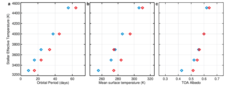
Figure 9: Here we show the rotation rate (a), mean surface temperature (b) and top-of-atmosphere albedo (c) for the last converged solutions found in this study. Blue diamonds are for low-metallicity stars, and red diamonds are for high-metallicity stars. Variability about the trend is due to the coarseness of our solar constant interval (50 or 100 W m^-2, depending on $T_{eff}$) across our simulation sets. The temperature of the last converged solution is much lower around redder stars, due to the stronger interaction of the SED with the near-IR water vapor bands. The trend in the TOA albedo is dominated by the effect of the orbital period, which controls thickness of the substellar cloud deck.

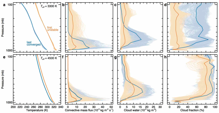
Figure 10: This plot shows vertical profiles of temperature (a, e), upward convective mass flux (b,f), grid-box averaged cloud water content (c,g), and cloud fraction (d,h) for the substellar region of the planet; (the elliptical region bounded by $\pm 30^{\circ}$ latitude and longitude from the substellar point). The top row is for planets around high-metallicity 3300 K stars, and the bottom row is for planets around high-metallicity 4500 K stars. Blue lines are for the last converged solution, red lines are for the first unstable simulation. The bolded lines are the mean of the substellar region. The light colored lines are from each individual profile within the substellar region. While the bifurcation is sharper around the 3300 K star, in both cases the first unstable simulation is characterized by a lessening of the lapse rate in the boundary layer and a reduction in substellar convection and thus in clouds.

3.5 Estimating water-loss to space

In section 3.3 we established new limits to the inner edge of the HZ based on the last converged solutions for stable climates. This criterion is intentionally taken to compare with inner HZ results for slow rotators in Yang et al. (2014). In section 3.4 we argue that the last converged solutions lie just below the threshold of an abrupt climatic transition towards hotter states, whereupon the substellar cloud deck weakens considerably and strong solar radiation then heats the planet. However, we have not yet considered the potential for significant water-loss from our modeled atmospheres. Notably, water-loss to space from a moist greenhouse is believed to be the more conservative estimate for inner edge of the HZ, and essentially a limit to habitability, occurring at a lower stellar flux (and thus further from the star) than does a runaway greenhouse.

At first glance, Fig. 9 appears to indicate that our model atmospheres located nearest the inner edge of the HZ are probably too cold to experience significant water-loss to space, all being below   310 K. Note that the canonical value for the mean surface temperature marking the moist greenhouse water-loss limit is 340 K in 1D models (Kasting et al. 1993; Kopparapu et al. 2013), and was recently found be to  350 K using CAM4 to simulate Earth under high stellar fluxes (Wolf & Toon, 2015). In Fig. 11 we show the model top (i.e. 3 mb) water vapor mixing ratio and the lifetime of the ocean against water-loss, assuming an initial water inventory equal to 1 Earth ocean ($1.4\times 10^{24}$g H₂O). We assume diffusion limited escape from the upper most model layer, following Hunten (1973). The solid red and solid blue lines in the Fig. 11b are the estimated main sequence lifetimes for high and low metallicity stars respectively. Interestingly, for nearly all our simulations that define the IHZ, even those with seemingly little water vapor in their upper atmospheres, the lifetime to lose an Earth ocean is approximately equal to or shorter than the main sequence lifetime of the host star. Of course, for M stars this timescale remains much larger than the current age of the universe, and thus is of little practical use for determining habitability.

However, synchronous rotators around late-K stars have significant water vapor near the model top and thus can have rapid water-loss rates. Our last converged solutions around stars with $T_{eff}=4500$K can lose an Earth ocean in less than 1 Gyr (red and blue diamonds in Fig. 11b, left-top). Thus these atmospheres may not be habitable under the more stringent water-loss criteria. The inner edge of the HZ defined by water-loss is thus likely at a lower stellar flux for late-K stars, compared with that illustrated in Fig 8. These atmospheres undergo rapid water-loss at a surprisingly low global mean surface temperature, between 295 K and 310 K. We postulate that strong substellar convection may be more effective at pumping water vapor into the high atmosphere, compared to tropical convection on a rapidly rotating world. However, there is much more work left to be done. Here, our model uses a relatively low model top, with poor resolution of the stratosphere. Furthermore, Yang et al. (2014), using CAM3 with an identical vertical resolution, found much lower water vapor mixing ratios in the upper atmosphere for an early (wet) Venus around the Sun. Future planned work will utilize a higher model top, with significantly improved vertical resolution, and will study a wider range of stellar fluxes.

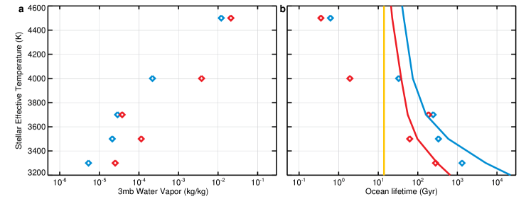
Figure 11: The model top (3 mb) water vapor volume mixing ratio (a) and the lifetime of an Earth ocean against diffusion limited water-loss (b). Blue and red diamonds are from the last converged solutions around low-metallicity stars high-metallicity stars respectively. The solid blue and red lines in panel (b) are the total main sequence lifetime for low-metallicity and high-metallicity stars respectively. The vertical yellow line in panel (b) is the current age of the universe.

3.6 Habitability of M-dwarfs

Several studies have argued that terrestrial planets within the HZs of M dwarfs may not be habitable, either because they could be deficient in volatiles (Lissauer, 2007) or form dry as a result of inefficient water delivery (Raymond et al., 2007), if they formed in situ. If the planets migrate from the outer parts of the system, they accumulate massive H and He envelopes. Whether they are able to shed most of their H-rich envelopes and potentially become ’habitable evaporated cores’ (HECs) depends on the mass of the solid core and the X-ray/UV-driven escape (Luger et al., 2015). Recently, Luger & Barnes (2015) pointed out that due to the extended pre-main sequence phase of M dwarfs ($\sim 100$Myr, Baraffe et al. (2015)), where the star is more luminous than its main sequence phase, terrestrial planets in the (current) HZs of M dwarfs could have been in runaway greenhouse during the pre-main sequence phase and may therefore be uninhabitable. This prolonged runaway greenhouse state may have removed water from a planet’s atmosphere through photolysis, and may dessicate the planet. As a by-product, if the surface of the planet is not an efficient oxygen sink, the resulting oxygen from the photolysis may accumulate and can potentially generate an abiotically produced bio-signature (Luger & Barnes, 2015). However, based on the combined results from planetary population synthesis and atmospheric water-loss models, Tian & Ida (2015) suggest a bimodel distribution of water contents for terrestrial planets around low mass stars. Earth-like water endowments may be rare, but dune and deep ocean worlds may both be common. Thus, the extended pre-main sequence phase of M-dwarfs does not unequivocally rule out the existence of ocean planets.

4 Conclusions

Low-eccentricity planets at the inner edge of the HZ around low-mass stars that are within the tidal locking radius and not perturbed by planetary companions are expected to be in synchronous rotation, with $1:1$ spin-orbit resonance. In this paper, we showed that to determine the inner edge of the HZ around low-mass stars using 3-D GCMs, care should be taken to self-consistently calculate the orbital/rotational periods of the planets as a function of the incident stellar flux, in accordance with Kepler’s third law. Previous GCM studies that assumed fixed, 60-day orbital periods were always in the slow-rotator dynamical regime, and thus may have overestimated fractional cloud cover and planetary albedo on planets near the inner edge of the HZ. According to our model, planets orbiting late-M dwarfs should begin transitioning to the fast-rotator regime, resulting in zonal banding and a decrease in cloud cover, with a corresponding decrease in planetary albedo. Thus, in our model the HZ inner edge moves outward for planets orbiting late M dwarfs compared to previous calculations. For hotter stars, though, ($T_{eff}>3700$ K), the inner edge moves inwards as a result of improved numerics in the CAM4 GCM.

We also showed that, for a given stellar $T_{eff}$, the location of the HZ for M-dwarfs depends on the metallicity of the star, because metallicity affects the stellar luminosity and hence, the semi-major axis and orbital period of a planet near the inner edge. Low-metallicity stars are more luminous for a given $T_{eff}$, and hence their HZ boundaries are farther out.

Future work will include updating the radiative transfer scheme in CAM4, and taking into account that water can become major atmospheric constituent on warm, moist planets. Still, these results are a first step towards improved estimates of the HZ inner edge. We encourage model intercomparisons, and all 3-D calculations of HZ boundaries should be validated by several independent GCMs, as is done routinely in the global climate change community.

References

- Anglada-Escude et al. (2013) Anglada-Escude, G., Tuomi, M., Gerlach, E. et al. 2013. A&A, 556, id.A126
- Baraffe et al. (2015) Baraffe, I., Homeier, D., Allard, F., & Chabrier, G. 2015. A&A, 577, id.A42
- Boyajian et al. (2012) Boyajian, T. S., Von Braun, K., Van Belle, G., et al. 2012. ApJ, 757, 112
- Boyajian et al. (2014) Boyajian, T. S., Van Belle, G., Braun, V. et al. 2014. AJ, 147, 47
- Carone et al. (2014) Carone L., Keppens, R., & Decin, L. (2014). MNRAS, 445, 930
- Chabrier & Baraffe (2000) Chabrier, G., & Baraffe, I. 2000. ARAA, 38, 337
- Dotter et al. (2008) Dotter, A., Chaboyer, B., Jevremovic, D., et al. 2008. ApJS, 178, 89
- Edson et al. (2011) Edson, A., Lee, S., Bannon, P. et al. 2011. Icarus, 212, 1
- Haqq-Misra & Kopparapu (2015) Haqq-Misra, J., & Kopparapu, R. K. 2015. MNRAS. 446, 428
- Heng & Vogt (2011) Heng, K., Vogt, S. 2011, MNRAS, 415, 2145
- Hunten (1973) Hunten, D. M. 1973. J. Atmos. Sci., 30, 1481
- Joshi et al. (1997) Joshi, M. M., Haberle R. M., Reynolds R. T. 1997. Icarus, 129, 450
- Kaspi & Showman (2015) Kaspi, Y., Showman, A. P. 2015. ApJ, 804, 60
- Kasting et al. (1993) Kasting, J., F., Whitmire, D., P., & Reynolds. R. T. 1993, Icarus, 101, 108
- Kopparapu et al. (2013) Kopparapu, R. K., Ramirez, R., Kasting, J. F., Eymet, V., Robinson, T. D., Mahadevan, S., Terrien, R. C., Domagal-Goldman, S. D., Meadows, V., & Deshpande, R. 2013, ApJ, 765, 131
- Kopparapu et al. (2014) Kopparapu, R. K., Ramirez, R. M., SchottelKotte, J. et al. 2014. ApJ, 787, L29
- Leconte et al. (2013) Leconte, J., Forget, F., Charnay, B., Wordsworth, R., & Pottier, A. 2013. Nature, 504, 268
- Leconte et al. (2015) Leconte, J., Wu, H., Menou, K., & Murray, N. 2015. Science, 347, 632
- Lissauer (2007) Lissauer, J. J. 2007. ApJ, 660, L149
- Luger & Barnes (2015) Luger. R., & Barnes, R. 2015. Astrobiology, 15, 2
- Luger et al. (2015) Luger. R., Barnes, R., Lopez, E., Fortney, J., Jackson, B., & Meadows, V. 2015. Astrobiology, 15, 57
- Mann et al. (2015) Mann, W. A., Feiden, A. G., Gaidos, E., Boyajian, T., & Von Braun, K. 2015. ApJ, 804, 64
- Neale et al. (2010) Neale, R. B., Gettelman, S. P., Chen, C. C. et al. 2010. NCAR/TN-486+STR NCAR TECHNICAL NOTE
- Newton et al. (2015) Newton, E., Charbonneau, D., Irwin, J., & Mann, A. 2015. ApJ, 800, 85
- Ricker et al. (2014) Ricker, G. R., Winn, J. N., Vanderspek, R. et al. 2014. Proceedings of the SPIE, 9143, 914320
- Raymond et al. (2007) Raymond, S. N., Scalo, J., Meadows, V. S. 2007. ApJ, 669, 606
- Robertson et al. (2014) Robertson, P., & Mahadevan, S. 2014. ApJ, 793, L24
- Selsis et al. (2007b) Selsis, F. et al. 2007b. A&A, 476, 137
- Sherwood & Huber (2010) Sherwood, S. C. & Huber, M. 2010. PNAS, 107(21), 9552
- Showman et al. (2013a) Showman, A. P.,Fortney. J. J., Lewis, N. K., Shabram, M. 2013. ApJ, 762, 24
- Showman et al. (2013) Showman, A.P., R.D. Wordsworth, T.M. Merlis, and Y. Kaspi. 2013. Comparative Climatology of Terrestrial Planets (S.J. Mackwell et al., Eds.), Univ. Arizona Press. pp. 277-326.
- Terrien et al. (2015) Terrien, R. C., Mahadevan, S., Bender, C. F., Deshpande, R., & Robertson, P. 2015. ApJ, 802, L10
- Tian & Ida (2015) Tian, F., & Ida, S. Nature Geoscience, 8, 177
- Way et al. (2015) Way, M. J., Del Genio, A. D., Kelley, M., Aleinov, I., Clune, T. 2015. Comparative Climatology of Terrestrial Planets II, NASA Conference Proceeding, arxiv:1511.07283
- Wolf & Toon (2014) Wolf, E., & Toon, E. 2014. Geophysical Research Letters. 41, doi:10.1002/2013GL058376
- Wolf & Toon (2015) Wolf, E., & Toon, E. 2015. JGRA, 120, 5775
- Wordsworth & Pierrehumbert (2013) Wordsworth, R., & Pierrehumbert, R. 2013. Science, 339, 64
- Yang et al. (2013) Yang, J., Cowan, N. B., & Abbot, D. S. 2013. ApJ, 771, L45
- Yang et al. (2014a) Yang, J., Gwenael, B., Fabrycky, D., & Abbot, D. 2014. ApJ, 787, L2
- Young et al. (2012) Young, P. A., Liebst, K., & Pagano, M. 2012. ApJ, 755, L31