A simple, general result for the variance of substitution number in molecular evolution.

Abstract

The number of substitutions (of nucleotides, amino acids, …) that take place during the evolution of a sequence is a stochastic variable of fundamental importance in the field of molecular evolution. Although the mean number of substitutions during molecular evolution of a sequence can be estimated for a given substitution model, no simple solution exists for the variance of this random variable.

We show in this article that the computation of the variance is as simple as that of the mean number of substitutions for both short and long times. Apart from its fundamental importance, this result can be used to investigate the dispersion index $R$, i.e. the ratio of the variance to the mean substitution number, which is of prime importance in the neutral theory of molecular evolution. By investigating large classes of substitution models, we demonstrate that although $R\geq 1$, to obtain $R$ significantly larger than unity necessitates in general additional hypotheses on the structure of the substitution model.

I Introduction.

Evolution at the molecular level is the process by which random mutations change the content of some sites of a given sequence (of nucleotides, amino acids, …) during time. The number of substitutions $n$ that occur during this time is of prime importance in the field of molecular evolution and its characterization is the first step in deciphering the history of evolution and its many branching. The main observable in molecular evolution, on comparing two sequences, is $\hat{p}$, the fraction of sites at which the two sequences are different. In order to estimate the statistical moments of $n$, the usual approach is to postulate a substitution model $\mathbf{Q}$ through which $\hat{p}$ can be related to the statistical moments of $n$. The simplest and most widely used models assume that $\mathbf{Q}$ is site independent, although this constraint can be relaxedGraur1999 ; Yang2006 .

Once a substitution model $\mathbf{Q}$ has been specified, it is straightforward to deduce the mean number of substitutions $\left\langle n\right\rangle$ and the process is detailed in many textbooks. However, the mean is only the first step in the characterization of a random variable and by itself is a rather poor indicator. The next step in the investigation of a random variable is to obtain its variance $V$. Surprisingly, no simple expression for $V$ can be found in the literature for arbitrary substitution model $\mathbf{Q}$. The first purpose of this article is to overcome this shortcoming. We show that computing $V$ is as simple as computing $\left\langle n\right\rangle$, both for short and long times.

We then apply this fundamental result to the investigation of the dispersion index $R$, the ratio of the variance to the mean number of substitutions. The neutral theory of molecular evolution introduced by KimuraKimura1984 supposes that the majority of mutations are neutral (i.e. have no effect on the phenotypic fitness) and therefore substitutions in protein or DNA sequences accumulate at a “constant rate” during evolution, a hypothesis that plays an important role in the foundation of the “molecular clock”Bromham2003 ; Ho2014 . The original neutral theory postulated that the substitution process is Poissonian, i.e. assuming $R=1$. Since the earliest work on the index of dispersion, it became evident however that $R$ is usually much larger than unity (see Cutler2000a for a review of data). Many alternatives have been suggested to reconcile the “overdispersion” observation with the neutral theory (Cutler2000a ). Among these various models, a promising alternative, that of fluctuating neutral space, was suggested by Takahata Takahata1991a which has been extensively studied in various frameworks (Zheng2001 ; Bastolla2002 ; Wilke2004 ; Bloom2007 ; Raval2007 ).

The fluctuating neutral space model states that the substitution rate $m_{j}^{i}$ from state $i$ to state $j$ is a function of both $i$ and $j$. States $i$ and $j$ can be nucleotides or amino acids, in which case we recover the usual substitution models of molecular evolution discussed above. The states can also be nodes of a neutral graph used to study global protein evolution (Huynen1996 ; Bornberg-Bauer1999 ; VanNimwegen1999 ). For neutral networks used in the study of protein evolution, Bloom, Raval and Wilke Bloom2007 devised an elegant procedure to estimate the substitution rates. We will show in this article that in general $R\geq 1$ and the equality is reached only for the most trivial cases. However, producing large $R$ requires additional hypotheses on the structure of substitution rates.

In summary, the problem we investigate in this article is to find a simple and general solution for the variance and dispersion index of any substitution matrix of dimension $K$. A substitution matrix $\mathbf{Q}$ collects the transition rates $m_{j}^{i}$ ($i\neq j$); its diagonal elements $q_{i}^{i}=-m^{i}$ are set such that its columns sum to zero (see below for notations) and designate the rate of leaving state $i$. Because of this condition, $\mathbf{Q}$ is singular.

Zheng Zheng2001 was the first to use Markov chains to investigate the variance of substitution number as a solution of a set of differential equations. His investigation was further developed by Bloom, Raval and Wilke Bloom2007 who gave the general solution in terms of the spectral decomposition of the substitution matrix; this solution was extended by Raval Raval2007 for a specific class of matrices used for random walk on neutral graphs. Minin and Suchard Minin2008 used the same spectral method to derive an analytical form for the generating function of a binary process.

The first step to characterize the substitution number, which as is well known, is to find the equilibrium probabilities $\pi_{i}$ of being in a state $i$, which is obtained by solving the linear system $\sum_{i}q_{j}^{i}\pi_{i}=0$ with the additional condition of $\sum_{i}\pi_{i}=1$. Once $\pi_{i}$ are obtained, the mean substitution number as a function of time is simply $\left\langle n\right\rangle=\bar{m}t$ where $\bar{m}=\sum_{i}m^{i}\pi_{i}$ is the weighted average of the “leaving” rates.

We show here that finding the variance necessitates a similar computation. Denoting the weighted deviation of the diagonal elements of $\mathbf{Q}$ from the mean $h_{i}=(\bar{m}-m^{i})\pi_{i}$, we have to find the solution of the linear system $\sum_{i}q_{j}^{i}r_{i}=h_{j}$ with the additional condition $\sum r_{i}=0$. For long times, the dispersion index is then simply

$$R=1+\frac{2}{\bar{m}}\sum_{i=1}^{K}m^{i}r_{i}$$ (1)

For short times, i.e. when the mean number of substitutions is small, the result is even simpler :

$$R=1+\frac{v_{m}}{\bar{m}^{2}}\left\langle n\right\rangle$$ (2)

where

$$v_{m}=\sum_{i=1}^{K}(\bar{m}-m^{i})^{2}\pi_{i}$$

in other words, $v_{m}$ is the variance of the diagonal elements of the substitution matrix, weighted by the equilibrium probabilities.

This article is organized as follow. In the next section, we use a Markov chain approach to derive relations (1,2) and show its validity by comparing it to results obtained by direct numerical simulations. The simplicity of these results then allows us to study the dispersion index for specific models of nucleotide substitutions widely used in the literature (section III) and for general models (section IV). We investigate in particular the conditions necessary to produce large $R$. The last section is devoted to a general discussion of these results and to conclusions. Technical details, such as the proof of $R\geq 1$ are given in the appendices.

II Markov chain model of dispersion index.

II.1 Background and definitions.

The problem we investigate in this article is mainly that of counting transitions of a random variable

Figure 1: The random variables $X$ can switch between $K$ states; the counter $N$ of the number of transitions is incremented at each transition of the variable $X$. The figure above shows one realization of these random variables as a function of time.

(figure 1). Consider a random variable $X$ that can occupy $K$ distinct states and let $m_{j}^{i}$ ($i\neq j$, $1\leq i,j\leq K$ ) be the transition rate from state $i$ to state $j$. The probability density $p_{i}(t)$ of being in state $i$ at time $t$ is governed by the Master equation

$$\frac{dp_{i}}{dt} = -\sum_{j}m_{j}^{i}p_{i}+\sum_{j}m_{i}^{j}p_{j}$$

$$= -m^{i}p_{i}+\sum_{j}m_{i}^{j}p_{j}$$

where $m^{i}=\sum_{j}m_{j}^{i}$ is the “leaving” rate from state $i$. We can collect the $p_{i}$ into a (column) vector $\left|p\right\rangle=(p_{1},...p_{K})^{T}$ and write the above equations in matrix notation

$$\frac{d}{dt}\left|p\right>=(-\mathbf{D}+\mathbf{M})\left|p\right>=\mathbf{Q}\left|p\right>$$ (3)

where $\mathbf{D}$ is the diagonal matrix of $m^{i}$ and $\mathbf{M}=(m_{j}^{i})$ collects the detailed transition rates from state $i$ to state $j$ ($i\neq j$) and has zero on its diagonal. In our notations, the upper (lower) index designates the column (row) of a matrix. The matrix $\mathbf{Q}=-\mathbf{D}+\mathbf{M}$ is called the substitution matrix and its columns sum to zero.

Before proceeding, we explain the notations used in this article. As the matrix $\mathbf{Q}$ is not in general symmetric, a clear distinction must be made between right (column) and left (row) vectors. The Dirac notations are standard and useful for handling this distinction : a column vector $(x_{1},...x_{K})^{T}$ is denoted $\left|x\right>$ while a row vector $(y^{1},...,y^{K})$ is denoted $\left<y\right|$ and $\left\langle y|x\right\rangle=\sum_{i}y^{i}x_{i}$ is their scalar product. In some of literature (see Yang2006 ), the substitution matrix is the transpose of the matrix used here and the master equation is then written as $d\left<p\right|/dt=\left<p\right|\mathbf{Q}$ and therefore its rows sum to zero.

By construction, the matrix $\mathbf{Q}$ is singular and has one zero eigenvalue while all others are negative. Therefore, as time flows, $\left|p(t)\right>\rightarrow\left|\pi\right>$ where $\left|\pi\right>=(\pi_{1},...\pi_{K})$ is the equilibrium occupation probability and the zero-eigenvector of the substitution matrix.

$$\mathbf{Q}\left|\pi\right> = 0$$

$$\left\langle 1|\pi\right\rangle = 1$$

where $\left<1\right|=(1,...1)$, and the second condition expresses that the sum of the probabilities must be 1. Note that by definition, $\left<1\right|\mathbf{Q}=0$, and thus $\left<1\right|$ is a zero left eigenvector of the substitution matrix.

II.2 Problem formulation.

To count the number of substitutions (figure 1), we consider the probability densities $p_{i}^{n}(t)$ of being in state $i$ after $n$ substitutions at time $t$. These probabilities are governed by the master equation

$$\frac{dp_{i}^{n}}{dt} = -m^{i}p_{i}^{n}+\sum_{j}m_{i}^{j}p_{j}^{n-1}\,\,\,\,\,\,n>0$$

$$\frac{dp_{i}^{0}}{dt} = -m^{i}p_{i}^{0}$$

We can combine the above equations by setting $p_{i}^{n}(t)=0$ if $n<0$. Collecting the elements of $(p_{1}^{n},p_{2}^{n},...,p_{K}^{n})^{T}$ into the vector $\left|p^{n}\right>$, the above equation can then be written as

$$\frac{d}{dt}\left|p^{n}\right>=-\mathbf{D}\left|p^{n}\right>+\mathbf{M}\left|p^{n-1}\right>$$ (4)

The quantities of interest for the computation of the dispersion index are the mean and the variance of the number of substitutions. The mean number of substitutions at time $t$ is

$$\left\langle n(t)\right\rangle=\sum_{i,n}np_{i}^{n}(t)$$

Let us define

$$n_{i}(t)=\sum_{n}np_{i}^{n}(t)$$

and collect the partial means $n_{i}$ into the vector $\left|n(t)\right>=(n_{1},...,n_{K})^{T}$. The mean is then defined simply as

$$\left\langle n(t)\right\rangle=\sum_{i}n_{i}(t)=\left\langle 1|n(t)\right\rangle$$

By the same token, the second moment

$$\left\langle n^{2}(t)\right\rangle=\sum_{i,n}n^{2}p_{i}^{n}(t)$$

can be written in terms of partial second moments $n_{i}^{2}=\sum_{n}n^{2}p_{i}^{n}(t)$ as

$$\left\langle n^{2}(t)\right\rangle=\left\langle 1|n^{2}(t)\right\rangle$$

where $\left|n^{2}(t)\right>=(n_{1}^{2},...,n_{K}^{2})^{T}$. It is straightforward to show (see appendix A), for the initial condition $\left|p^{n}(0)\right\rangle=\left|\pi\right\rangle$, that $\left|n(t)\right>$ and $\left|n^{2}(t)\right>$ obey a linear differential equation

$$\frac{d}{dt}\left|n\right> = \mathbf{Q}\left|n\right>+\mathbf{D}\left|\pi\right>$$ (5)

$$\frac{d}{dt}\left|n^{2}\right> = \mathbf{Q}\left|n^{2}\right>+2\mathbf{M}\left|n\right>+\mathbf{D}\left|\pi\right>$$ (6)

Let us define the left vector

$$\left<m\right|=(m^{1},...,m^{K})$$

which collects the leaving rates. By definition, $\left<1\right|\mathbf{M}=\left<1\right|\mathbf{D}=\left<m\right|$. Multiplying eqs (5,6) by the left vector $\left<1\right|$, and noting that $\left<1\right|\mathbf{Q}=\left<0\right|$, we get a simple relation for the moments :

$$\frac{d}{dt}\left\langle n\right\rangle = \left\langle m|\pi\right\rangle$$ (7)

$$\frac{d}{dt}\left\langle n^{2}\right\rangle = 2\left\langle m|n\right\rangle+\left\langle m|\pi\right\rangle$$ (8)

We observe that the mean number of substitutions involves only a trivial integration. Defining the weighted average of the leaving rates as

$$\bar{m}=\left\langle m|\pi\right\rangle=\sum_{i}m^{i}\pi_{i}$$

the mean number of substitution is simply

$$\left\langle n(t)\right\rangle=\bar{m}t$$ (9)

To compute the second moment of the substitution number on the other hand, we must solve for $\left|n\right>$ using equation (5) and then perform one integration. The next subsection is devoted to the efficient solution of this procedure.

II.3 Solution of the equation for the moments .

One standard way of solving equation (5) would be to express the matrix $\mathbf{Q}$ in its eigenbasis; equation(5) is then diagonalized and can be formally solved. This is the method used by Bloom, Raval and Wilke Bloom2007 and further refined by RavalRaval2007 for a specific class of substitution matrices where $m_{j}^{i}=0\,\mbox{or}\,1$. The first problem with this approach is that there is no guarantee that $\mathbf{Q}$ is diagonalizable. Even if $\mathbf{Q}$ can be diagonalized, this is not the most efficient procedure to find $V$, as it necessitates the computation of all eigenvalues and left and right eigenvectors of $\mathbf{Q}$ and then the cumbersome summation of their binomial products.

The procedure we follow involves some straightforward, albeit cumbersome linear algebraic operations, but the end result is quite simple. We note that the matrix $\mathbf{Q}$ is singular and has exactly one zero eigenvalue, associated with the left $\left<1\right|$ and right $\left|\pi\right>$ eigenvectors. The method we use is to isolate the zero eigenvalue by making a round-trip to a new basis. Thus, if we can find a new basis in which the substitution matrix $\mathbf{Q}^{\prime}=\mathbf{X}^{-1}\mathbf{Q}\mathbf{X}$ takes a lower block triangular form

$$\mathbf{Q}^{\prime}=\left(\begin{array}[]{c|c}0&0\cdots 0\\ \hline\cr&\raisebox{-12.91663pt}{{\large\mbox{{$\mathbf{\tilde{Q}}$}}}}\\[-14.2083pt] \tilde{\alpha}&\\[-2.15277pt] &\end{array}\right)$$ (10)

we will have achieved our goal of isolating the zero eigenvalue. The non singular matrix $\mathbf{\tilde{\mathbf{Q}}}$ is of rank $K-1$ and has the non-zero and negative eigenvalues of $\mathbf{Q}$. As $\left<1\right|$ is the known left eigenvalue of $\mathbf{Q}$, we can split the vector space into ${\cal B}=\{\left|u\right\rangle$| $\left\langle 1|u\right\rangle=0\}$ and the space padded by $\left|\pi\right\rangle$. It is then straightforward to find the above transfer matrices $\mathbf{X}$ and $\mathbf{X}^{-1}$ for such a transformation:

$$\mathbf{X}=\left(\begin{array}[]{ccccc}1&-1&-1&\cdots&-1\\ 0&1&0&\cdots&0\\ 0&0&1&\cdots&0\\ \vdots&&&\ddots&\vdots\\ 0&&\cdots&0&1\end{array}\right);\mathbf{X}^{-1}=\left(\begin{array}[]{ccccc}1&1&1&\cdots&1\\ 0&1&0&\cdots&0\\ 0&0&1&\cdots&0\\ \vdots&&&\ddots&\vdots\\ 0&&\cdots&0&1\end{array}\right)$$

Under such a transformation, a right vector $\left|x\right\rangle=(x_{1},x_{2},...,x_{K})^{T}$ transforms into

$$\left|x^{\prime}\right\rangle=\mathbf{X}^{-1}\left|x\right\rangle=\left(\begin{array}[]{c}\sum_{i}x_{i}\\ x_{2}\\ \vdots\\ x_{K}\end{array}\right)=\left(\begin{array}[]{c}\sum_{i}x_{i}\vspace{0.5ex}\\ \hline\cr\\ \left|\tilde{x}\right\rangle\\ \\ \end{array}\right)$$

where the $K-1$ dimensional vector $\left|\tilde{x}\right\rangle=(x_{2},...,x_{K})^{T}$. In general, we will designate by a $\tilde{}$  all vectors that belong the $K-1$ dimensional space ${\cal B}$ in which the linear application $\mathbf{\tilde{Q}}$ operates.

A left vector $\left<y\right|=(y^{1},y^{2},...,y^{K})$ transforms into

$$\left<y^{\prime}\right|=\left<y\right|\mathbf{X}=(y^{1},y^{2}-y^{1},...,y^{K}-y^{1})=(y^{1}\vline\ \left<\tilde{y}\right|\ )$$

where the $K-1$ dimensional left vector $\left<\tilde{y}\right|=(y^{2}-y^{1},...,y^{K}-y^{1})$.

Finally, $\tilde{Q}_{j}^{i}=Q_{j}^{i}-Q_{j}^{1}$ where the elements of $\tilde{\mathbf{Q}}$ have been indexed from 2 to $K$.

Expressing now the equation (5) for the evolution of first moments in the new basis, we find that

$$\frac{d}{dt}\left\langle n\right\rangle = \bar{m}$$ (11)

$$\frac{d}{dt}\left|\tilde{n}\right\rangle = \mathbf{\tilde{Q}}\left|\tilde{n}\right\rangle+\left\langle n\right\rangle\left|\tilde{\alpha}\right\rangle+\left|\tilde{\mu}\right\rangle$$ (12)

where $\left|\tilde{n}\right\rangle=(n_{2},...,n_{K})^{T}$, $\left|\tilde{\mu}\right\rangle=(m^{2}\pi_{2},...,m^{K}\pi_{K})$ and $\left|\tilde{\alpha}\right\rangle$ is given in relation 10. Equation (11) is the same as equation (7) and implies that $\left\langle n\right\rangle=\bar{m}t$. As $\tilde{\mathbf{Q}}$ is non-singular (and negative definite), equations (11,12) can now readily be solved. Noting that $\mathbf{Q}\left|\pi\right\rangle=0$ implies that $\left|\tilde{\alpha}\right\rangle+\tilde{\mathbf{Q}}\left|\tilde{\pi}\right\rangle=0$, the differential equation (12) integrates

$$\left|\tilde{n}\right\rangle=\left(\mathbf{I}-e^{\tilde{\mathbf{Q}}t}\right)\tilde{\mathbf{Q}}^{-1}\left|\tilde{h}\right\rangle+\left\langle n\right\rangle\left|\tilde{\pi}\right\rangle$$ (13)

where $\left|\tilde{h}\right\rangle=\bar{m}\left|\tilde{\pi}\right\rangle-\left|\tilde{\mu}\right\rangle$.

To compute the second moment (equation 8) and the variance, we need must integrate the above expression one more time. We finally obtain

$$\mbox{Var}(n) = \left\langle n^{2}\right\rangle-\left\langle n\right\rangle^{2}$$

$$= \left\langle n\right\rangle+2\left\langle\tilde{m}|\left(It+\tilde{\mathbf{Q}}^{-1}(\mathbf{I}-e^{\tilde{\mathbf{Q}}t})\right)\tilde{\mathbf{Q}}^{-1}|\tilde{h}\right\rangle$$

The second term in the r.h.s. of the above equation is the excess variance $\delta V$ with respect to a Poisson process.

II.3.1 Long time behavior.

As all eigenvalues of $\tilde{\mathbf{Q}}$ are negative, for large times $\exp(\tilde{\mathbf{Q}}t)\rightarrow 0$ and the leading term of the excess variance is therefore

$$\delta V=2\left\langle\tilde{m}|\tilde{r}\right\rangle t$$ (15)

where $\left|\tilde{r}\right\rangle$ is the solution of the linear equation

$$\tilde{\mathbf{Q}}\left|\tilde{r}\right\rangle=\left|\tilde{h}\right\rangle$$ (16)

Returning to the original basis, relation (15) becomes

$$\delta V=2\left\langle m|r\right\rangle t$$ (17)

where $\left<m\right|=(m^{1},m^{2},...m^{K})$ is the left vector of the leaving rates and $\left|r\right\rangle$ is the solution of the linear equation

$$\mathbf{Q}\left|r\right\rangle = \left|h\right\rangle$$ (18)

$$\left\langle 1|r\right\rangle = 0$$ (19)

$\left|h\right\rangle=(h_{1},...,h_{K})^{T}$ is the vector of weighted deviation from $\bar{m}$ of the leaving rates $m^{i}$:

$$h_{i}=(\bar{m}-m^{i})\pi_{i}$$

Finally, for large times, the dispersion index is

$$R=1+2\frac{\left\langle m|r\right\rangle}{\bar{m}}$$ (20)

which is the relation (1) given in the introduction.

Figure 2 shows the agreement between the above theoretical results and stochastic numerical simulations.

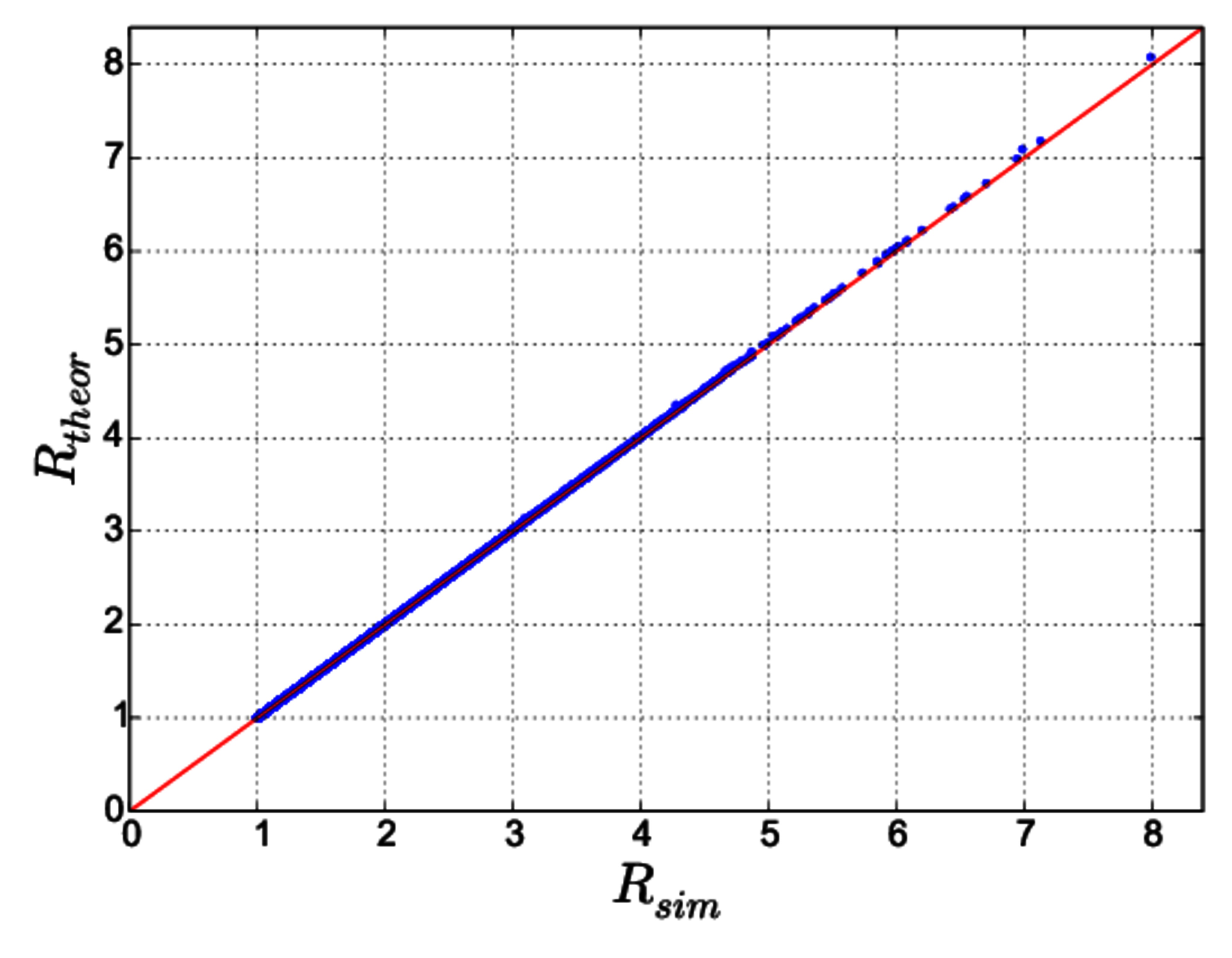
Figure 2: Comparison between the theoretical result (20) and numerical simulations. $3\times 10^{5}$ $4\times 4$ random (uniform$(0,1)$ ) matrices were generated. For each matrix, a Gillespie algorithm was used to generate $10^{6}$ random paths as a function of time ($t_{final}=1000$), from which the dispersion index was computed. In the above figure, each dot corresponds to one random matrix. The mean relative error $(R_{\mbox{theor}}-R_{\mbox{sim}})/R_{\mbox{theor}}$ is $1.3\times 10^{-3}$.

Two important consequences should be noted. First, it is not difficult to show that $R\geq 1$, which is called the overdispersion of the molecular clock. A demonstration of this theorem for symmetric substitution matrices whose elements are 0 or 1 (adjacency matrices) was given by Raval Raval2007 . We give the general demonstration for general time reversible (GTR) substitution matrices in appendix B .

The second consequence of relation (20) is that if all diagonal elements of the substitution matrix are equal (i.e. $m^{i}=m^{j}$ $\forall i,j$ ), then the dispersion index is exactly 1 and we recover the property of a normal Poisson process, regardless of the fine structure of $\mathbf{Q}$ and the equilibrium probabilities $\pi_{i}$. This is a sufficient condition. We show that the necessary condition for $R=1$ is $\left|h\right\rangle=\left|0\right\rangle$, which, except for the trivial case where some $\pi_{i}=0$, again implies the equality of diagonal elements of $\mathbf{Q}$ (see B).

II.3.2 Short time behavior.

For short times, i.e. when the mean number of substitution is small, we can expand $\delta V$ given by expression (II.3) to the second order in time:

$$\delta V = -t^{2}\left\langle\tilde{m}|\tilde{h}\right\rangle+O(t^{3})$$ (21)

$$= -t^{2}\sum_{i=2}^{K}(m^{i}-m^{1})(\bar{m}-m^{i})\pi_{i}+O(t^{3})$$ (22)

Note that the above summation is over $i=2\cdots K$ . However, by definition,

$$\sum_{i=1}^{K}(\bar{m}-m^{i})\pi_{i}=0$$

and hence the sum in relation (22) can be rearranged as

$$\delta V=t^{2}\sum_{i=1}^{K}(\bar{m}-m^{i})^{2}\pi_{i}$$ (23)

The sum,which we will denote by $v_{m}$, represents the variance of the diagonal elements of $\mathbf{Q}$, weighted by the equilibrium probabilities. It is more meaningful to express the variance in terms of the mean substitution number. Using relation (9), we therefore have

$$\delta V=\frac{v_{m}}{\bar{m}^{2}}\left\langle n\right\rangle^{2}$$ (24)

The dispersion index for short times is therefore

$$R=1+\frac{v_{m}}{\bar{m}^{2}}\left\langle n\right\rangle$$

The dispersion index for all times can also be computed, and an example is given in appendix C. In the next section, we investigate some applications of the relation (20).

III Application to specific nucleotides substitution models.

Nucleotide substitution models are widely used in molecular evolutionYang2006 ; Graur1999 for example to deduce distances between sequences. Some of these models have few parameters or have particular symmetries. For these models, it is worthwhile to express relation (20) for large times into an even more explicit form and compute the dispersion number as an explicit function of the parameters. We provide below such a computation for some of the most commonly used models.

For the K80 model proposed by KimuraKimura1980 , all diagonal elements of the substitution matrix are equal; hence, relation (20) implies that $R=1$.

III.1 T92 model.

Tamura TAMURA1992 introduced a two parameter model (T92) extending the K80 model to take into account biases in G+C contents. Solving relation (20) explicitly for this model, we find for the dispersion index

$$R=1+\frac{2k^{2}}{k+1}\frac{\theta(1-\theta)(2\theta-1)^{2}}{1+2k\theta(1-\theta)}$$ (25)

Here $k=\alpha/\beta$, where $\alpha$ and $\beta$ are the two parameters of the original T92 model. A similar expression was found by ZhengZheng2001 . For a given $k$, the maximum value of $R$ is

$$R^{*} = 1+\frac{\left(\sqrt{2+k}-\sqrt{2}\right)^{2}}{k+1}$$

And it is straightforward to show that in this case

$$R\in[1,2]$$

although even reaching a maximum value for $R=1.5$ will necessitate strong asymmetries in the substitution rates (such as $k=18.8$ and $\theta=0.063$).

III.2 TN93 model.

Tamura and NeiTamura1993 proposed a generalization of the F81Felsenstein1981 and HKY85 Hasegawa1985 models which allows for biases in the equilibrium probabilities, different rates of transition vs transversion and for different rates of transitions. The corresponding substitution matrix is

$$\mathbf{Q}_{\mbox{TN93}}=\mbox{$\mu$}\left(\begin{array}[]{cccc}*&k_{1}\pi_{1}&\pi_{1}&\pi_{1}\\ k_{1}\pi_{2}&*&\pi_{2}&\pi_{2}\\ \pi_{3}&\pi_{3}&*&k_{2}\pi_{3}\\ \pi_{4}&\pi_{4}&k_{2}\pi_{4}&*\end{array}\right)$$

a specific case of this model where $k_{1}=k_{2}$ corresponds to the HKY85 model, while $k_{1}=k_{2}=1$ corresponds to that of F81 (also called “equal input” ). Solving equation (20) leads to

$$R=1+\frac{2}{\bar{m}}\sum_{i<j}C_{ij}(m^{i}-m^{j})^{2}$$ (26)

where $m^{i}$ are the (negative of) diagonal elements of $\mathbf{Q}$, $\bar{m}=\sum_{i}m^{i}\pi_{i}$; $C_{ij}$ are defined as

$$C_{12} = \pi_{1}\pi_{2}\frac{1-(k_{1}-1)(\pi_{3}+\pi_{4})}{1+(k_{1}-1)(\pi_{1}+\pi_{2})}$$

$$C_{34} = \pi_{3}\pi_{4}\frac{1-(k_{2}-1)(\pi_{1}+\pi_{2})}{1+(k_{2}-1)(\pi_{3}+\pi_{4})}$$

$$C_{ij} = \pi_{i}\pi_{j}\,\,\,\,\mbox{for other}\,i,j$$

For the specific case $k_{1}=k_{2}=1$ (equal input or F81 model), expression (26) takes a particularly simple form

$$R = 1+\left(\sum_{i<j}\pi_{i}\pi_{j}(\pi_{i}-\pi_{j})^{2}\right)/\left(\sum_{i<j}\pi_{i}\pi_{j}\right)$$ (27)

$$= 1+2\frac{\sum_{i}\pi_{i}^{3}-\left(\sum_{i}\pi_{i}^{2}\right)^{2}}{1-\sum_{i}\pi_{i}^{2}}$$ (28)

One can deduce relation (27) from (28) by noting that $\sum_{i}\pi_{i}=1$. As every term of the first sum in relation (27) is smaller than the corresponding term in the second sum:

$$R_{\mbox{F81}}\in[1,2]$$

The lower bound is reached for $\left|\pi\right\rangle=(1/4)(1,1,1,1)^{T}$, while the upper bound is reached when one of the $\pi_{i}$ approaches 1. Zheng Zheng2001 has also computed an expression for the dispersion index for the F81 model; his solution however is rather complicated.

For the general TN93, relation $R\leq 2$ no longer holds. For example, for $\left|\pi\right\rangle=(0.6-\epsilon,\epsilon,0.2,0.2$), the dispersion index is

$$R_{\mbox{TN}}=0.04+0.24k_{2}+6/(6+k_{2})+O(\epsilon)$$

and $R$ can become arbitrarily large with appropriate values of $k_{2}$.

The simplicity of relation (26) allows for the comprehensive exploration of the hyperplane $\sum_{i}\pi_{i}=1$ , $\pi_{i}>0$. The results are displayed in figure 3 ; to obtain large values for $R$ such as $R>1.5$ necessitates high asymmetries in the transition rates and/or strong biases in equilibrium probabilities of states .

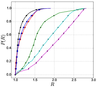
Figure 3: Cumulative histogram of the dispersion index $R$ of the TN93 model and its specific cases. The three dimensional space $\left|\pi\right\rangle=(\pi_{1},\pi_{2},\pi_{3},\pi_{4})$, $\sum_{i}\pi_{i}=1$ is scanned by steps of $d\pi=0.025$ ($\approx 11200$ points). For each value of $\left|\pi\right\rangle$, the dispersion index of the corresponding substitution matrix $\mathbf{Q}_{\mbox{TN93}}$ is computed from relation (21). Black circles : the F81 model ($k_{1}=k_{2}=1)$; red diamonds and green left triangles correspond the HKY85 with respectively $k_{1}=k_{2}=0.1$ and $10$; blue squares, cyan right triangles and magenta up triangles correspond to TN93 model with $\{k_{1},k_{2}\}=\{0.1,1\},\{1,10\},\{0.1,10\}$ respectively. Permutations of $\{k_{1},k_{2}\}$ lead to the same results and are not displayed. For each substitution matrix, it has been checked that solution (26) and the general solution (20) are identical.

IV Statistical investigation of the dispersion index and the influence of sparseness.

The relation (20) can be solved explicitly for general substitution matrices. However, a general substitution matrix of dimension 4 has 11 free parameters (substitution matrices are defined up to a scaling parameter); explicit solution of (20) as a function of substitution matrix parameters is rather cumbersome and does not provide insightful information.

An exchangeable (time reversible, GTR) substitution matrix has the additional constraintTavare1986 $m_{j}^{i}\pi_{i}=m_{i}^{j}\pi_{j}$. Considering only exchangeable matrices reduces the number of free parameters to 9, but the parameter space is still too large to be explored systematically.

We can however sample the parameter space by generating a statistically significant ensemble of substitution matrices $\mathbf{Q}$ and get an estimate of the probability distribution of the dispersion index $R$. The simplicity of relation (20) allows us to generate $10^{7}$ random matrices for each class (see section VI) and compute their associated $R$ in a few minutes with a usual normal computer : depending on the dimension of $\mathbf{Q}$ (from 4 to 20) this computation takes between 2 and 10 minutes.

Figure 4.a shows the cumulative probability $P(R)$ for both arbitrary (R) and GTR (G) matrices, computed from $10^{7}$ matrices in each case. We observe that arbitrary matrices produce statistically low dispersal indices : $P(R>1.5)=0.08$ and $P(R>3)=2.7\times 10^{-3}$. The GTR matrices have statistically higher dispersion indices: $P(R>1.5)=0.495$ and $P(R>3)=0.048$. Still, values larger than $R=5$, as has been reported in the literatureCutler2000a , have a very low probability ($1.4\times 10^{-4}$ for random matrices and $7\times 10^{-3}$ for GTR matrices).

We observed in the preceding section that for each class of matrices, high values of $R$ are generally associated with large biases in the equilibrium probabilities, i.e. a given state would have a very low equilibrium probability in order to allow for large $R$. We can investigate how this observation holds for general and GTR matrices. For each $K\times K$ matrix $\mathbf{Q}$ that is generated we quantify its relative eccentricity by

$$e=K\,\mbox{min}_{i}(\pi_{i})$$

The relation between $R$ and $e$ is statistical: matrices with dispersion index in $[R,R+dR]$ will have a range of $e$ and we display the average $e$ for each small interval (Figure 4.b). We observe again that high values of the dispersion index in each class of matrices requires high bias in equilibrium probabilities of states.

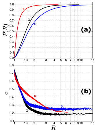
Figure 4: Statistical study of $4\times 4$ substitution matrices for (i) GTR matrices (“G”,black curves) ; (ii) arbitrary matrices (“R”, red curves) and (iii) sparse GTR matrices (“S”, blue curves). In each case, $10^{7}$ matrices are generated and for each matrix, its dispersion index $R$ and its eccentricity $e=\mbox{min}(\pi_{i})$ are computed, where $\pi_{i}$ is the equilibrium probability of state $i$. In each case, the data are sorted by $R$ value to compute the cumulative histogram (a). figure (b) shows the relation between $e$ and $R$. To make visible the statistical relation between $e$ and $R$, a moving average of size 1000 data points is applied to the $10^{7}$sorted $(R,e)$ data in each data set and the result $(R_{m},e_{m})$ is displayed in the lower plot (b).

Another effect that can increase the dispersion index of a matrix is its sparseness. This effect was investigated by Raval Raval2007 for a random walk on neutral networks, which we generalize here. Until now, we have examined fully connected graphs, i.e. substitution processes where the random variable $X$ can jump from any state $i$ to any other state $j$. For a 4 states random variable, each node of the connectivity graph is of degree 3 ($d_{G}=3$). This statement may however be too restrictive. Consider for example a $4\times 4$ nucleotide substitution matrix for synonymous substitutions. Depending on the identity of the codon to which it belongs, a nucleotide can only mutate to a subset of other nucleotides. For example, for the third codon of Tyrosine, only $\mbox{T}\leftrightarrow\mbox{C}$ transitions are allowed, while for the third codon of Alanine, all substitutions are synonymous. For a given protein sequence, the mean nucleotide synonymous substitution graph is therefore of degree smaller than 3. In general, the degree of each state (node) $i$ is given by the number (minus one) of non-zero elements of the $i-$th column in the associated substitution matrix.

We can investigate the effect of sparseness of substitution matrices on the dispersion index with the formalism developed above. Figure 4 shows the probability distribution of $R$ for GTR matrices with $d_{G}=2$. As it can be observed, the dispersion index distribution for GTR matrices is shifted to higher values and $P(R>5)$ increases six fold from 0.007 (for $d_{G}=3)$ to 0.044 (for $d_{G}=2$).

The effect of sparseness can be investigated better by considering higher dimensional substitution matrices. Consider a random variable $X$ that can take 16 different values. Figure 5 shows the effect of sparseness of $\mathbf{Q}$ on the distribution of the dispersion index. We have considered GTR matrices in three cases : (i) fully connected transition graphs ($d_{G}=15$) ; (ii) regular graphs of degree 4 where two different states $i,j=1$…16 are connected if their binary representations are one mutation apart ; and (iii) regular graphs of degree 2. For each class, $10^{7}$ matrices are generated. As can be observed, the sparseness shifts the dispersion index distribution to the right : the median in the three cases is respectively 1.65, 2.08 and 6.15.

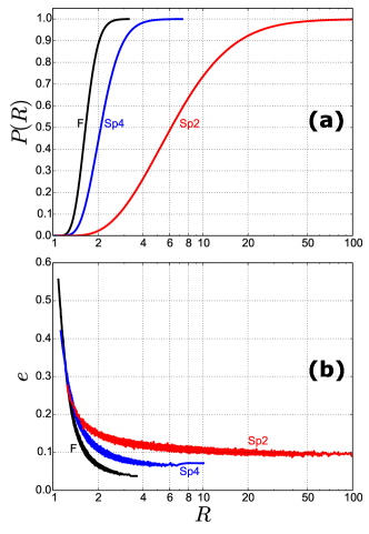
Figure 5: Effect of sparseness of $16\times 16$ GTR substitution matrices, for three different connectivities. For each class, $10^{7}$ random matrices are generated and their statistical properties displayed . Black lines (marked F) : fully connected graphs $d_{G}=15$ ; blue lines (marked Sp4) $d_{G}=4$ ; red lines (marked Sp4) $d_{G}=2$. (a) The cumulative probability $P(R)$ for each class. (b) the mean eccentricity as a function of dispersion index for each class.

A more insightful model would be $20\times 20$ GTR matrices for amino acid substitutions. We compare the case of fully connected graphs (F) where any amino acid can replace any other one to the case where only amino acids one nucleotide mutation apart can replace each other (non-synonymous substitution, NS). The average degree of the graph in the latter case is $\bar{d}_{G}=7.5$. As before, we generate $10^{7}$ random matrices in each class and compute their statistical properties. We observe again (Figure 6) that the distribution of $R$ is shifted to the right for the NS graphs, where the median is $R_{\mbox{NS}}=2.48$, compared to $R_{\mbox{F}}=1.66$ for fully connected graphs.

For specific amino acid substitution matrices used in the literature such as WAGWhelan2001 , LGLe2008 and IDRSzalkowski2011 , the index of dispersion is 1.253, 1.196 and 1.242 respectively.

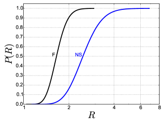
Figure 6: Cumulative probability of the dispersion index for Fully connected (black, F) and non-synonymous (blue, NS) amino acid $20\times 20$ substitution matrix. For the fully connected matrix, any amino acid can be replaced by any other. For the NS matrices, only amino acids one nucleotide mutation apart can replace each other. For each case, $10^{7}$ $20\times 20$ GTR matrices are generated and their dispersion index $R$ are computed. For the NS matrices, transitions are weighted by the number of nucleotide substitutions that can lead from one amino acid to another: there are for example 6 nucleotide mutations that transform a Phenylalanine into a Leucine, but only one mutation that transforms a Lysine into a Isoleucine.

V Discussion and conclusion.

The substitution process (of nucleotides, amino acids, …) and therefore the number of substitutions $n$ that take place during time $t$ are stochastic. One of the most fundamental task in molecular evolutionary investigation is to characterize the random variable $n$ from molecular data.

A given model for the substitution process in the form of a substitution matrix $\mathbf{Q}$ enables us to estimate the mean number of substitution $\left\langle n\right\rangle$ that occur during a time $t$. The mean depends only on the diagonal elements of $\mathbf{Q}$ and the equilibrium probabilities of states $\pi_{i}$:

$$\left\langle n(t)\right\rangle=-tQ_{i}^{i}\pi_{i}=-t\mbox{\,tr}(\mathbf{Q}\Pi)$$ (29)

where tr() designates the trace operator.

In molecular evolution, the main observable is the probability $p_{d}(t)$ that two different sequences are different at a given site. Denoting $\mathbf{U}(t)=\exp(t\mathbf{Q})$, and assuming that both sequences are at equilibrium Yang2006 ,

$$p_{d}(t)=1-U_{i}^{i}\pi_{i}=1-\mbox{tr}(\mathbf{U}\Pi)$$ (30)

One can estimate $p_{d}(t)$ from the fraction of observed differences between two sequences $\hat{p}$. By eliminating time in relations (29,30), it is then possible to relate the estimators $\hat{d}$ (of $\left\langle n\right\rangle$) and $\hat{p}$

$$\hat{d}=f(\hat{p})$$ (31)

For sequences of length $L$, $\hat{p}$ is given by a binomial distribution $B(L,p)$ and the variance of the distance estimator $\hat{d}$ can be deduced from relation (31). This quantity however is very different from the intrinsic variance of the substitution number.

The mean of substitution number, its estimator $\hat{d}$ and the variance of the estimator are only the first step in characterizing a random variable. The next crucial step is to evaluate the variance $V$ of this number. What we have achieved in this article is to find a simple expression for $V$. In particular, we have shown that for both short and long time scales, the variance $V$ can be easily deduced from $\mathbf{Q}$. For long times, the procedure is similar to deriving the equilibrium probabilities $\pi_{i}$ from $\mathbf{Q},$ i.e. we only need to solve a linear equation associated with $\mathbf{Q}$ (relation 17). For short times, only the diagonal elements of $\mathbf{Q}$ are required to compute $V$ (relation 23).

A long standing debate in the neutral theory of evolution concerns the value of dispersion index $R=V/\left\langle n\right\rangle$. On the one hand, the exact solution of this paper is used to demonstrate that in general, any substitution process given by a matrix $\mathbf{Q}$ is overdispersed, i.e. $R\geq 1$, and the equality can be observed only for trivial models where all diagonal elements of $\mathbf{Q}$ are equal. On the other hand, comprehensive investigation of various substitution models (section III,IV) shows that models that produce $R$ much larger than $\approx 2$ generally require strong biases in the equilibrium probabilities of states. One possibility to produce a higher dispersion index is sparse matrices, where the ensemble of possible transitions has been reduced.

The substitution models we have considered here can be applied to sequences where the $\mathbf{Q}$ matrix is the same for all sites. For nucleotide sequences, this can describe the evolution of non-coding sequences or synonymous substitutions (by taking into account the sparseness of the matrix). On the other hand, for amino acid substitution, it is well known that some sites are nearly constant or evolve at a slower pace than other sites. A natural extension of the present work would be to take into account substitution matrices that vary among sites, drawing for example their scaling factor from a Gamma distribution Yang2006 . The formalism we have developed in this article can be readily adapted to such an extension and the variance of the substitution number can be computed for variable substitution matrices.

VI Methods.

Numerical simulation of stochastic equations use the Gillespie algorithm Gillespie1977 and are written in C++ language. To compute the dispersion index of a given matrix $\mathbf{Q}$, we generate $10^{6}$ random path over a time period of 1000. To compare the analytical solutions given in this article (figure 2) to stochastic simulations (figure 2), we generated $3.6\times 10^{5}$ random matrices and numerically computed their dispersion index by the above method. This numerical simulation took approximately 10 days on a 60 core cluster.

All linear algebra numerical computations and all data processing were performed with the high-level Julia language Bezanson2014 . Computing the analytical dispersion index for the above $3.6\times 10^{5}$ random matrices took about 5 seconds on a normal desktop computer, using only one core.

To generate random GTR matrices, we use the factorization $\mathbf{Q}=\mathbf{S}\Pi^{-1}$ (see appendix B) which allows for independent generation of the $K(K-1)/2$ elements of the symmetric matrix $\mathbf{S}$ and $K-1$ elements of $\Pi$. For arbitrary matrices, we draw the $K(K-1)$ elements of the matrix. All random generator used in this work are uniform(0,1).

Acknowledgments.

We are grateful to Erik Geissler, Olivier Rivoire and Ivan Junier for fruitful discussions and critical reading of the manuscript.

Appendix A Mean and variance equation.

Obtaining equations of the moments such as (7,8) from the Master equation is a standard procedure of stochastic processesGardiner2004 ; Houchmandzadeh2009a . We give here the outline of the derivation.

Consider the master equation (4)

$$\frac{d}{dt}\left|p^{n}\right>=-\mathbf{D}\left|p^{n}\right>+\mathbf{M}\left|p^{n-1}\right>$$ (32)

which is a system of $K$ equations for the $p_{i}^{n}(t)$, written in vectorial form. Multiplying each row by $n$ and summing over all $n$ leads, in vectorial form, to

$$\frac{d}{dt}\sum_{n}\left|np^{n}\right>=-\mathbf{D}\sum_{n}\left|np^{n}\right>+\mathbf{M}\sum_{n}\left|np^{n-1}\right>$$

The term $\sum_{n}\left|np^{n}\right>$ was defined as the vector of the partial means $\left|n\right>$. For the second term, we have

$$\sum_{n}\left|np^{n-1}\right>=\sum_{n}\left|(n+1)p^{n}\right>=\left|n\right>+\left|p\right>$$ (33)

where $\left|p\right>=\sum_{n}\left|p^{n}\right>$ is the probability density of the random variable $X$ being in state $i$, whose dynamics is given by relation (3). For the initial condition $\left|p(0)\right>=\left|\pi\right>$, we have at all times

$$\left|p(t)\right>=\left|\pi\right>$$

so the moment equation is

$$\frac{d}{dt}\left|n\right>=(-\mathbf{D}+\mathbf{M})\left|n\right>+\mathbf{M}\left|\pi\right>$$

which is relation (5). Note that by definition, $\mathbf{M}\left|\pi\right>=\mathbf{D}\left|\pi\right>$.

The equation for the second moment (8) is obtained by the same procedure where each row of equation (32) is multiplied by $n^{2}$. Higher moments and the probability generating function equations can be obtained by similar computations.

Appendix B Proof of over dispersion for GTR substitution matrices.

As we have seen in relation (20), the dispersion index for long times is

$$R=1+2\frac{\left\langle m|r\right\rangle}{\bar{m}}$$

We must demonstrate that $\left\langle m|r\right\rangle\geq 0$ to prove that $R\geq 1$. We give here the proof for GTR matrices. These matrices can be factorized into

$$\mathbf{Q}=\mathbf{S}.\mathbf{\Pi^{-1}}$$ (34)

where $\Pi=\mbox{diag}(\pi_{1},...,\pi_{k})$ and $\mathbf{S}$ is a symmetric matrix of positive non-diagonal elements whose columns (and rows) sum to zero. Note that in the literatureYang2006 , a slightly different factorization is used in the form of $\mathbf{Q}=\Pi.\mathbf{F}$, where $\mathbf{F}$ is a symmetric matrix (we stress again that in our notation, the substitution matrix is the transpose of that used in most of the literature). The advantage of the factorization (34) is that except for one zero eigenvalue, all other eigenvalues of $\mathbf{S}$ are negative. $\mathbf{S}$ can be therefore be written as

$$\mathbf{S}=\sum_{i=2}^{K}\lambda_{i}\left|v_{i}\right\rangle\left\langle v_{i}\right|$$ (35)

where $\left|v_{i}\right\rangle$ and $\left\langle v_{i}\right|$ are the right and left orthonormal eigenvectors of $\mathbf{S}$ associated with the eigenvalue $\lambda_{i}$. The pseudo-inverse of $\mathbf{S}$ is defined as

$$\tilde{\mathbf{S}}^{-1}=\sum_{i=2}^{K}\lambda_{i}^{-1}\left|v_{i}\right\rangle\left\langle v_{i}\right|$$ (36)

and it is strictly negative definite .

The vector $\left|r\right\rangle$ is the solution of the linear equation

$$\mathbf{Q}\left|r\right\rangle = \left|h\right\rangle$$ (37)

$$\left\langle 1|r\right\rangle = 0$$ (38)

where $h_{i}=(\bar{m}-m^{i})\pi_{i}$. The general solution of the undetermined equation (37) is therefore

$$\left|r\right\rangle=C\left|\pi\right\rangle+\Pi\tilde{\mathbf{S}}^{-1}\left|h\right\rangle$$

where the constant $C$ is determined from the condition (38). On the other hand

$$\left\langle m\right| = \left\langle m\right|-\bar{m}\left\langle 1\right|+\bar{m}\left\langle 1\right|$$

$$= -\left\langle h\right|\Pi^{-1}+\bar{m}\left\langle 1\right|$$

And thus

$$\left\langle m|r\right\rangle = -\left\langle h|\Pi^{-1}|r\right\rangle+\bar{m}\left\langle 1|r\right\rangle$$ (39)

$$= -\left\langle h|\tilde{\mathbf{S}}^{-1}|h\right\rangle-C\left\langle h|1\right\rangle$$

$$= -\left\langle h|\tilde{\mathbf{S}}^{-1}|h\right\rangle$$

where we have used the fact that $\left\langle 1|r\right\rangle=\left\langle 1|h\right\rangle=0$. As $\tilde{\mathbf{S}}^{-1}$ is negative definite ,

$$\left\langle m|r\right\rangle\geq 0$$

Moreover, the equality is reached only when $\left|h\right\rangle=\left|0\right\rangle$, i.e. for $\pi_{i}\neq 0$, only when all diagonal elements of $\mathbf{Q}$ are equal. To see this, we can expand relation (39)

$$\left\langle m|r\right\rangle=-\sum_{i=2}^{K}\lambda_{i}^{-1}\left\langle v_{i}|h\right\rangle^{2}$$

The only way to obtain $\left\langle m|r\right\rangle=0$ is to have $\left\langle v_{i}|h\right\rangle=0$ for $i=2..K$. As on the other hand, $\left\langle v_{1}|h\right\rangle=\left\langle 1|h\right\rangle=0$ we must have $\left|h\right\rangle=\left|0\right\rangle$.

Appendix C Dispersion index for all times.

In subsection II.3 we gave the long (eq. 20) and short (eq.24) time solution of the variance. For all the specific models used in the literature (section III), the variance at all times can also be determined explicitly through relation (II.3)

$$\delta V=2\left\langle\tilde{m}|\left(It+\tilde{\mathbf{Q}}^{-1}(\mathbf{I}-e^{\tilde{\mathbf{Q}}t})\right)\tilde{\mathbf{Q}}^{-1}|\left|\tilde{h}\right\rangle\right\rangle$$ (40)

The procedure requires the computation of $\exp(\mathbf{Q}t)$ and is analogous to the determination of $\left\langle n\right\rangle$ from sequence dissimilaritiesYang2006 ; Zheng2001 .

As an example, consider the equal input model (F81) which we studied in subsection III.2. For this model, the reduced matrix is simply

$$\tilde{\mathbf{Q}}=-\mu\mathbf{I}_{3}$$

where $\mbox{{I}}_{3}$ is the $3\times 3$ identity matrix and therefore $\exp(\tilde{\mathbf{Q}}t)=\exp(-\mu t)\mathbf{I}_{3}$. Relation (40) then becomes

$$\delta V =- \frac{2}{\mu^{2}}(-1+\mu t+e^{-\mu t})\left\langle\tilde{m}|\tilde{h}\right\rangle$$

We have previously shown (eq. 23) that generally

$$-\left\langle\tilde{m}|\tilde{h}\right\rangle=\sum_{i=1}^{K}(\bar{m}-m^{i})^{2}\pi_{i}=v_{m}$$

and for the F81 model,

$$\mu^{-2}v_{m}=\sum_{i=1}^{K}\pi_{i}^{3}-\left(\sum_{i=1}^{K}\pi_{i}^{2}\right)^{2}$$

However, the time can be expressed as a function of mean the substitution number. Finally, for the F80 model, and setting $\mu=1$ without loss of generality, the dispersion index for all times is

$$R(\left\langle n\right\rangle)=1+2\left(\frac{\left\langle n\right\rangle}{\bar{m}}+e^{-\left\langle n\right\rangle/\bar{m}}-1\right)\frac{v_{m}}{\left\langle n\right\rangle}$$

References

- [1] Dan Graur and Wen-Hsiung Li. Fundamentals of Molecular Evolution. Sinauer Associates Inc.,U.S, 1999.
- [2] Ziheng Yang. Computational molecular evolution. Oxford series in ecology and evolution, 2006.
- [3] Motoo Kimura. The Neutral Theory of Molecular Evolution. Cambridge University Press, 1984.
- [4] Lindell Bromham and David Penny. The modern molecular clock. Nature reviews. Genetics, 4(3):216–24, mar 2003.
- [5] Simon Y W Ho and Sebastián Duchêne. Molecular-clock methods for estimating evolutionary rates and timescales. Molecular ecology, 23(24):5947–65, dec 2014.
- [6] D J Cutler. The index of dispersion of molecular evolution: slow fluctuations. Theoretical population biology, 57(2):177–86, mar 2000.
- [7] Naoyuki Takahata. Statistical models of the overdispersed molecular clock. Theoretical Population Biology, 39(3):329–344, jun 1991.
- [8] Qi Zheng. On the dispersion index of a Markovian molecular clock. Mathematical Biosciences, 172(2):115–128, aug 2001.
- [9] Ugo Bastolla, Markus Porto, H Eduardo Roman, and Michele Vendruscolo. Lack of self-averaging in neutral evolution of proteins. Physical review letters, 89(20):208101, nov 2002.
- [10] Claus O Wilke. Molecular clock in neutral protein evolution. BMC genetics, 5(1):25, aug 2004.
- [11] Jesse D Bloom, Alpan Raval, and Claus O Wilke. Thermodynamics of neutral protein evolution. Genetics, 175(1):255–66, jan 2007.
- [12] Alpan Raval. Molecular clock on a neutral network. Physical review letters, 99(13):138104, sep 2007.
- [13] M. A. Huynen, P. F. Stadler, and W. Fontana. Smoothness within ruggedness: the role of neutrality in adaptation. Proceedings of the National Academy of Sciences, 93(1):397–401, jan 1996.
- [14] E. Bornberg-Bauer and H. S. Chan. Modeling evolutionary landscapes: Mutational stability, topology, and superfunnels in sequence space. Proceedings of the National Academy of Sciences, 96(19):10689–10694, sep 1999.
- [15] E. van Nimwegen, J. P. Crutchfield, and M. Huynen. Neutral evolution of mutational robustness. Proceedings of the National Academy of Sciences, 96(17):9716–9720, aug 1999.
- [16] Vladimir N Minin and Marc A Suchard. Counting labeled transitions in continuous-time Markov models of evolution. Journal of mathematical biology, 56(3):391–412, mar 2008.
- [17] Motoo Kimura. A simple method for estimating evolutionary rates of base substitutions through comparative studies of nucleotide sequences. Journal of Molecular Evolution, 16(2):111–120, jun 1980.
- [18] K Tamura. Estimation of the number of nucleotide substitutions when there are strong transition-transversion and G+C-content biases. Molecular biology and evolution, 9(4):678–687, jul 1992.
- [19] K Tamura and M Nei. Estimation of the number of nucleotide substitutions in the control region of mitochondrial DNA in humans and chimpanzees. Mol. Biol. Evol., 10(3):512–526, may 1993.
- [20] Joseph Felsenstein. Evolutionary trees from DNA sequences: A maximum likelihood approach. Journal of Molecular Evolution, 17(6):368–376, nov 1981.
- [21] M Hasegawa, H Kishino, and T Yano. Dating of the human-ape splitting by a molecular clock of mitochondrial DNA. Journal of molecular evolution, 22(2):160–174, 1985.
- [22] Simon Tavaré. Some Probabilistic and Statistical Problems in the Analysis of DNA Sequences. Lectures in Mathematics in the Life Sciences, 17:57, 1986.
- [23] S. Whelan and N. Goldman. A General Empirical Model of Protein Evolution Derived from Multiple Protein Families Using a Maximum-Likelihood Approach. Molecular Biology and Evolution, 18(5):691–699, may 2001.
- [24] Si Quang Le and Olivier Gascuel. An improved general amino acid replacement matrix. Molecular biology and evolution, 25(7):1307–20, jul 2008.
- [25] Adam M Szalkowski and Maria Anisimova. Markov models of amino acid substitution to study proteins with intrinsically disordered regions. PloS one, 6(5):e20488, jan 2011.
- [26] Daniel T Gillespie. Exact stochastic simulation of coupled chemical reactions. The Journal of Physical Chemistry, 81(25):2340–2361, 1977.
- [27] Jeff Bezanson, Alan Edelman, Stefan Karpinski, and Viral B. Shah. Julia: A Fresh Approach to Numerical Computing. page 37, nov 2014.
- [28] C Gardiner. Handbook of Stochastic Methods: for Physics, Chemistry and the Natural Sciences. Springer, 2004.
- [29] Bahram Houchmandzadeh. Theory of neutral clustering for growing populations. Physical Review E, 80(5):051920, nov 2009.