The Fe ii emission in active galactic nuclei:
excitation mechanisms and location of the emitting region

Abstract

We present a study of Fe ii emission in the near-infrared region (NIR) for 25 active galactic nuclei (AGNs) to obtain information about the excitation mechanisms that power it and the location where it is formed. We employ a NIR Fe ii template derived in the literature and found that it successfully reproduces the observed Fe ii spectrum. The Fe ii bump at 9200Å detected in all objects studied confirms that Ly$\alpha$ fluorescence is always present in AGNs. The correlation found between the flux of the 9200Å bump, the 1 $\mu$m lines and the optical Fe ii imply that Ly$\alpha$ fluorescence plays an important role in the Fe ii production. We determined that at least 18$\%$ of the optical Fe ii is due to this process while collisional excitation dominates the production of the observed Fe ii. The line profiles of Fe ii $\lambda$10502, O i $\lambda$11287, Ca ii $\lambda$8664 and Pa$\beta$ were compared to gather information about the most likely location where they are emitted. We found that Fe ii, O i and Ca ii have similar widths and are, on average, 30$\%$ narrower than Pa$\beta$. Assuming that the clouds emitting the lines are virialized, we show that the Fe ii is emitted in a region twice as far from the central source than Pa$\beta$. The distance though strongly varies: from 8.5 light-days for NGC 4051 to 198.2 light-days for Mrk 509. Our results reinforce the importance of the Fe ii in the NIR to constrain critical parameters that drive its physics and the underlying AGN kinematics as well as more accurate models aimed at reproducing this complex emission.

1. Introduction

The broad line region (BLR) in active galactic nuclei (AGNs) has been extensively studied from X-rays to the near infrared region (NIR) during the last decades (see Gaskell, 2009, for a review) but several aspects about its physical properties remain under debate. That is the case of the Fe ii emission, whose numerous multiplets form a pseudo-continuum that extends from the ultraviolet (UV) to the NIR due to the blending of over 344,000 transitions (Bruhweiler $\&$ Verner, 2008) although it is not clear that even that number of lines could denote adequate coverage. This emission is significant for at least four reasons: (i) it represents one of the most conspicuous cooling agents of the BLR, emitting about 25% of the total energy of this region (Wills et al., 1985); (ii) it represents a strong contaminant because of the large number of emission lines. Without proper modeling and subtraction, it may lead to a wrong description of the BLR physical conditions; (iii) the gas responsible for the Fe ii emission can provide important clues on the structure and kinematics of the BLR and the central source. However, despite the extensive study of the Fe ii emission, (Kuehn et al., 2008; Matsuoka et al., 2008; Popović et al., 2007; Sluse et al., 2007; Hu et al., 2008; Kovačević et al., 2010) the strong blending of the lines prevents an accurate study of its properties and excitation mechanisms; (iv) The strength of Fe ii relative to the peak of [O iii], the so called eigenvector 1, which consists of the dominant variable in the principal component analysis presented by Boroson $\&$ Green (1992), is believed to be associated to important parameters of the accretion process (Sulentic et al., 2000; Boroson $\&$ Green, 1992).

Due to its complexity and uncertainties in transition probabilities and excitation mechanisms, the most successful approach to model the Fe ii emission in AGNs consists of deriving empirical templates from observations. Among the most successful templates for the optical region are the ones of Boroson $\&$ Green (1992) and Véron-Cetty et al. (2004), which were developed using the spectrum of I Zw 1, the prototype of NLS1 that is widely known for its strong iron emission in the optical and UV regions (Joly, 1991; Lawrence et al., 1997; Rudy et al., 2000; Tsuzuki et al., 2006; Bruhweiler $\&$ Verner, 2008). Other works also successfully employ templates to quantify the optical Fe ii emission in larges samples of AGNs (Tsuzuki et al., 2006; Popović et al., 2007; Kovačević et al., 2010; Dong et al., 2010, 2011). For the UV region, Vestergaard $\&$ Wilkes (2001) extended the Fe ii template using Hubble Space Telescope/FOS spectra of I Zw 1, presenting the first UV template for this emission.

Two decades after the seminal work by Boroson $\&$ Green (1992) on the optical FeII emission template, the first semi-empirical NIR FeII template was derived by Garcia-Rissmann et al. (2012) using a mid-resolution spectrum of I Zw 1 and theoretical models of Sigut et al. (2004) and Sigut $\&$ Pradhan (2003). They successfully modeled the Fe ii emission in that galaxy as well as Ark 564, another NLS1 known for its conspicuous iron emission (Joly, 1991; Rodríguez-Ardila et al., 2002). Similar to the optical, they found that the Fe ii spectrum in the NIR forms a subtle pseudo-continuum that extends from 8300 Å up to 11800 Å. However, unlike in the optical, the NIR Fe ii spectrum displays prominent lines that can be fully isolated, allowing the characterization of Fe ii emission line profiles and its comparison to other BLR emission features. That property confers an advantage to the NIR over the optical, making the Fe ii emission in that region a powerful tool to study and understand this complex emission. It can be used, for instance, to observationally constrain the most likely location of the region emitting this ion. Previous works in the NIR carried out on a few targets (Rodríguez-Ardila et al., 2002) suggest that the Fe ii lines are preferentially formed in the outer part of the BLR. Studies on a larger number of sources are necessary to confirm this trend and compare it to results obtained in the optical (Kovačević et al., 2010; Popović et al., 2007; Boroson $\&$ Green, 1992).

Despite the wide and successful use of templates to reproduce, measure and subtract the Fe ii emission in AGNs (Boroson $\&$ Green, 1992; Vestergaard $\&$ Wilkes, 2001; Véron-Cetty et al., 2004; Garcia-Rissmann et al., 2012), attempts on determining the mechanisms that drive this emission continue to be an open issue. Current models (Baldwin et al, 2004; Verner et al., 1999; Bruhweiler $\&$ Verner, 2008) include processes such as continuum fluorescence, collisional excitation and self-fluorescence among Fe ii transitions. They are successful at reproducing the emission lines strengths for the UV and optical lines but results for the NIR are not presented, very likely because the relevant transitions in that region are not included. Penston (1987) proposed that Ly$\alpha$ fluorescence could be a key process involved in the production of Fe ii. Indeed, models developed by Sigut $\&$ Pradhan (1998, 2003) and Sigut et al. (2004) showed that this mechanism is of fundamental importance in determining the strength of Fe ii in the NIR. The key feature that would reveal the presence of such mechanism is the detection of the Fe ii blend at 9200 Å, first identified by Rodríguez-Ardila et al. (2002) in AGNs. The bulk of this emission would be produced by primary cascades from the upper 5p levels to e⁴D and e⁶D levels after a capture of a Ly$\alpha$ photon.

Additional NIR features resulting from secondary cascading after the Ly$\alpha$ fluorescence process are the so-called 1 $\mu$m Fe ii lines ($\lambda$9997, $\lambda$10502, $\lambda$10862 and $\lambda$11127), which are the most prominent Fe ii features in the whole 8000-24000 Å region (Sigut $\&$ Pradhan, 2003; Pradhan $\&$ Nahar, 2011). The importance of the 1 $\mu$m lines resides in the fact that they are produced by the decay of the e⁴D and e⁶D levels down to the z⁴D⁰ and z⁴F⁰ levels. Transitions downwards from the latter two populate the upper levels responsible for nearly 50% of all optical Fe ii emission (Véron-Cetty et al., 2004). If Ly$\alpha$ fluorescence plays a key role as excitation mechanism of Fe ii in AGNs, a direct correlation should be observed between the strength of 9200 Å blend and the 1 $\mu$m Fe ii lines in the NIR. This issue should be investigated in detail because it can provide useful constrains to the Fe ii problem.

In this paper, we describe for the first time a detailed application of the semi-empirical NIR Fe ii template developed by Garcia-Rissmann et al. (2012) to a sample of 25 AGNs. The aims are threefold: (i) Provide a reliable test for the NIR Fe ii template and verify its capability to reproduce the numerous Fe ii emission lines in a sample of Type 1 AGNs. (ii) Measure the NIR Fe ii flux and compare it to that of the optical region to confirm model predictions of the role of Ly$\alpha$ fluorescence in the total Fe ii strength. (iii) Compare the Fe ii emission line profiles with other broad line features to probe the BLR structure and kinematics.

This paper is structured as follows: Section 2 describes the observations and data reduction. Section 3 presents the methodology adopted to convolve the NIR Fe ii template and its application to the galaxy sample and results. Section 4 discusses the excitation mechanisms of the NIR Fe ii emission. Section 5 discusses the kinematics of the BLR based on the Fe ii lines and other BLR emission as well the distance of the Fe ii emitting line region. Conclusions are given in Section 6.

2. Observations and data reduction

The 25 AGNs that compose our sample were selected primarily from the list of Joly (1991), who collected data for about 200 AGNs (Seyfert 1 and quasars) to study the relationship between Fe ii and radio emission. Additional selection criteria were applied to that initial sample such as the targets have to be brighter than K=12 mag to obtain a good compromise between signal-to-noise (S/N) and exposure time for the NASA 3 m Infrared Telescope Facility (IRTF) atop Mauna Kea. We also applied the restriction that the FWHM of the broad H$\beta$ component of the galaxies be smaller than 3000 km s^-1 in order to avoid severe blending of the Fe ii lines with adjacent permitted and forbidden features. Because of the last criterion, our final sample was naturally dominated by narrow-line Seyfert 1 galaxies. Basic information for the galaxy sample is listed in Table 1.

The NIR observations and data reduction for the above sample will be described first. Non-contemporaneous optical and UV spectroscopy obtained mostly from archival data (as well as pointed observations) were also collected for most sources of the sample for the purpose of assessing the optical and UV Fe ii emission. Since the data reduction of these latter data were described elsewhere we will discuss here only their sources and any particular issue we found interesting to mention.

2.1. Near-Infrared data

NIR spectra were obtained at IRTF from April 2002 to June 2004. The SpeX spectrograph (Rayner et al., 2003), was used in the short cross-dispersed mode (SXD, 0.8-2.4 $\mu$m). In all cases, the detector employed consisted of a 1024$\times$1024 ALADDIN 3 InSb array with a spatial scale of 0.15$\arcsec$/pixel. A 0.8$\times$15 slit was used giving a spectral resolution of 360 km s^-1. This value was determined both from the arc lamp spectra and the sky line spectra and was found to be constant with wavelength within 3%. During the different nights, the seeing varied between 0.7-1$\arcsec$. Observations were done nodding in an ABBA source pattern along the slit with typical integration times from 120 s to 180 s per frame and total on-source integration times between 35 and 50 min. Right before/after the science frames, an A0V star was observed near each target to provide a telluric standard at similar airmass. It was also used to flux calibrate the corresponding object.

The spectral reduction, extraction and wavelength calibration procedures were performed using SPEXTOOL, the in-house software developed and provided by the SpeX team for the IRTF community (Cushing et al., 2004). 1-D spectra were extracted using an aperture window of 0.8$\arcsec$ in size, centered at the peak of the light distribution. Because all objects of the sample are characterized by a bright central nucleus compared with the galaxy disk, the light profile along the spatial direction was essentially point-like. Under this assumption, SPEXTOOL corrects for small shifts due to atmospheric diffraction in the position of the light peak along the different orders.

The extracted galaxy spectra were then corrected for telluric absorption and flux calibrated using Xtellcor (Vacca et al., 2003), another in-house software developed by the IRTF team. Finally, the different orders of each science spectrum were merged to form a single 1-D frame. It was later corrected for redshift, determined from the average $z$ measured from the positions of [S iii] 9531 Å, Pa$\delta$, He i 10830 Å, Pa$\beta$ and Br$\gamma$. Galactic extinction corrections, as determined from the COBE/IRAS infrared maps of Schlegel et al. (1998), were applied for each target. The value of the Galactic E(B-V) used for each galaxy is listed in Col. 6 of Table 1.

2.2. Optical and Ultraviolet data

Optical spectroscopy for a sub-sample of objects were obtained from different telescopes, including archival data from SDSS and HST, as well as our own observations. Column 2 of Table 2 lists the source of the optical spectroscopy. The purpose of this spectra is to determine the integrated flux of the Fe ii blend centered at 4570 Å and H$\beta$ as well as R₄₅₇₀, the flux ratio Fe ii $\lambda$4570/H$\beta$.

In addition, UV spectroscopy for a sub-sample of sources taken with HST is also employed to compare the emission line profiles of Fe ii and other BLR features, including some high-ionization permitted lines.

As our interest is in the emission line spectrum, it is necessary to remove the strong continuum emission in the optical and NIR, assumed to be primarily from the central engine. To this purpose, we fit a polynomial function to the observed continuum using as anchor points regions free of emission lines and subtract it from the spectrum. Figure 1 shows an example of this procedure applied to 1H 1934-063A. This procedure proved to be successful to our purposes. The analysis of the individual continuum components (i.e., AGN, dust and stellar population) are beyond the scope of this paper, so no effort was made at interpreting the physical meaning of the fit.

In none of the cases the NIR and optical/UV spectroscopy were contemporaneous. Therefore, no effort was made to match the continuum emission in the overlapping regions of the spectra (i.e., NIR and optical and UV and optical) because of variability, seeing and aperture effects. However, since the optical data is used to provide quantities to be compared to the NIR, it is important to consider variability effects on the emission lines that are being analyzed. Few works in the literature, though, have found optical Fe ii variability, and the overall statistics are scarce.

Giannuzzo $\&$ Stirpe (1996), for example, reported variations of the Fe ii bump at 5200 Å of less than 15$\%$. Dietrich et al. (1993) detected no significant variations in the Fe ii lines in NGC 5548. Bischoff $\&$ Kollatschny (1999) found that optical Fe ii lines remained constant over a 10 year monitoring campaign, even when the Balmer lines and continuum were seen to vary over a range of 2 to 5. Wang et al. (2005) found that the Fe ii variations in NGC 4051 correlate with variations in the continuum and the H$\beta$ line. Similar results were found by Shapovalova et al. (2012) for Ark 564.

Few AGNs show strong Fe ii variations (larger than 50$\%$), particularly in very broad line objects (FWHM of H$\beta>4000$ km s^-1; Kollatschny et al., 1981; Kollatschny $\&$ Fricke, 1985; Kollatschny et al., 2000). For example, Kuehn et al. (2008) carried out a reverberation analysis of Ark 120. They were unable to measure a clean reverberation lag for this object. Barth et al. (2013), though, detected Fe ii reverberation for two broad line AGNs, Mrk 1511 and NGC 4593, using data from the LICK AGN Monitoring Project. They found variability with an amplitude lower than 20$\%$ relative to the mean flux value. In addition, Hu et al. (2015) report the detection of significant Fe ii time lags for a sample of 9 NLS1 galaxies in order to study AGNs with high accretion rates. Difficulties in detect variations in the Fe ii bump at $\lambda$4570 are usually ascribed to residual variations of the He ii $\lambda$4686, which is blended with Fe ii in this wavelength interval (Kollatschny $\&$ Dietrich, 1996).

The general scenario that emerges from these works is that the amplitude of the Fe ii variability (when it varies) in response to continuum variations is much smaller than that of H$\beta$. Indeed, this latter line is widely known to respond to continuum variability (Kaspi et al., 2000; Peterson et al., 2004, 1998; Kollatschny et al., 2000, 2006). Kollatschny et al. (2006) analyzed this effect using a sample of 45 AGNs in order to study the BLR structure. Considering the mean values of all fractional variabilities presented in their work as representative of the variability effect in our sample, we estimate an uncertainty of $\sim$11$\%$ on the optical fluxes due to variability. This value is also in good agreement with the results of Hu et al. (2015), which found an average fractional variability of 10$\%$ for Fe ii when compared with H$\beta$. This value is within the error in the line fluxes measured in this work; therefore, we conclude that variability is unlike to impact our results.

3. Analysis Procedure

3.1. NIR Fe ii Template Fitting

Modeling the Fe ii pseudo-continuum, formed by the blending of the thousands of Fe ii multiplets, remains a challenge for the analysis of this emission since it was first observed by Wampler $\&$ Oke (1967). Sargent (1968) noted that I Zw 1, for instance, had the same kind of emission but with stronger and narrower lines. The strength of the Fe ii lines in that AGN mades it a prototype of the strong Fe ii emitters as well as of the NLS1 subclass of AGNs, leading to the development of empirical templates of this emission based on this source (Boroson $\&$ Green, 1992; Vestergaard $\&$ Wilkes, 2001; Véron-Cetty et al., 2004; Garcia-Rissmann et al., 2012).

Sigut $\&$ Pradhan (2003) and Sigut et al. (2004) presented the first Fe ii model from the UV to the NIR using an iron atom with 827 fine structure energy levels and including all known excitation mechanisms (continuum fluorescence via the UV resonance lines, self-fluorescence via overlapping Fe ii transitions, and collisional excitation) that were traditionally considered by Wills et al. (1985) and Baldwin et al (2004) in addition to fluorescent excitation by Ly$\alpha$ as suggested by Penston (1987). Their models incorporates photoionization cross sections (references in Sigut et al., 2004) that include a large number of autoionizing resonances, usually treated as lines but too numerous to count explicitly, which means that they include many more photo-excitation transitions than the 23,000 bound-bound lines and would form part of the pseudo-continuum. Moreover, in their work they show how the Fe ii intensity varies as a function of the ionization parameter ($U_{\rm ion}$), the particle density ($n_{H}$) and the microturbulence velociy ($\zeta_{t}$). Details of all the physics involved in the calculations are in Sigut $\&$ Pradhan (2003). Landt et al. (2008) were the first to confront these models with observations, noting some discrepancies between the model and the observed emission lines. Bruhweiler $\&$ Verner (2008) using an Fe ii model with 830 energy levels (up to 14.06 eV) and 344,035 atomic transitions, found that the model parameters that best fit the observed UV spectrum of I Zw 1 were $log(\Phi_{H})=20.5$, $log(n_{H})=11.0$ cm^-3 and $\zeta_{t}$=20 km s^-1. Garcia-Rissmann et al. (2012) modeled the observed NIR spectrum of I Zw 1 using a grid of Sigut $\&$ Pradhan’s templates covering several values of ionization parameters and particle densities, keeping the microturbulence velocity constant at $\zeta_{t}$=10 km s^-1. They found that the model with $U_{\rm ion}$=$-2.0$ (implying in $log(\Phi_{H})=21.1$) and $log(n_{H})$=$12.6$ cm^-3 best fit the observations. Note that these values are comparable to those found by Bruhweiler $\&$ Verner (2008), suggesting that the physical conditions of the clouds emitting Fe ii are similar.

The template developed by Garcia-Rissmann et al. (2012) is composed of 1529 Fe ii emission lines in the region between 8300 Å and 11600 Å. In order to apply it to other AGNs, it is first necessary to convolve it with a line profile that is representative of the Fe ii emission. At this point we are only interested in obtaining a mathematical representation of the empirical profiles. In order to determine the optimal line width, we measured the FWHM of individual iron lines detected in that spectral region. We assumed that each Fe ii line could be represented by a single or a sum of individual profiles and that the main source of line broadening was the Doppler effect.

The Fe ii emission lines $\lambda$10502 and $\lambda$11127 are usually isolated and allow an accurate characterization of their form and width. The LINER routine (Pogge $\&$ Owen, 1993), a $\chi^{2}$ minimization algorithm that fits up to eight individual profiles (Gaussians, Lorentzians, or a linear combination of them as a pseudo-Voigt profile) to a single or a blend of several line profiles, was used in this step. We found that a single Gaussian/Lorentzian profile was enough to fit the two lines above in all objects in the sample. However, the difference between the rms error for the Gaussian and Lorentzian fit was less than 5%, which lies within the uncertainties. As Fe ii $\lambda$11127 is located in a spectral region with telluric absorptions, residuals left after division by the telluric star may hamper the characterization of that line profile. For this reason, we considered Fe ii $\lambda$10502 as the best representation of the broad Fe ii emission. Note that Garcia-Rissmann et al. (2012) argued that the Fe ii $\lambda$11127 is a better choice than Fe ii $\lambda$10502 because the latter can be slightly broadened due to a satellite Fe ii line at $\lambda$10490. However, Fe ii $\lambda$10490 is at least 5 times weaker relative to $\lambda$10502 (Garcia-Rissmann et al., 2012; Rodríguez-Ardila et al., 2002). Therefore, we adopted the $\lambda$10502 line as representative of the Fe ii profile because it can be easily isolated and displays a good S/N in the entire sample. The flux and FWHM measured for this line are shown in Columns 2 and 3 of Table 3.

For each object, a synthetic Fe ii spectrum was created from the template using the FWHM listed in Table 3 and then scaled to the integrated line flux measured for the $\lambda$10502 line.

In order to ensure that the line width used to convolve the template best represented the FWHM of the Fe ii emission region, we generated for each galaxy a grid of 100 synthetic spectra with small variations in the line width (up to 10% around the best value) for 3 different functions (Gaussian, Lorentzian and Voigt). In all cases, the value of the FWHM ​​that minimized the rms error after subtraction of the template was very close (less than 1%) to the width found from the direct measurement of the $\lambda$10502 line. Also, the best profile function found in all cases was the same one that fitted initially. The final parameters of the convolution of the template for each source are shown in Table 4.

Figures 2 to 5 show the observed spectra and the template convolved with the best parameters (upper panel). The ion-free spectra after subtraction of the modeled Fe ii emission are shown in the bottom panels. It can be seen that overall the template nicely reproduces the observed Fe ii in all AGNs. We measure the rms error of the subtraction of the template using as reference the regions around the 1 $\mu$m lines. The mean rms error of the template subtraction are shown in column 4 of Table 4.

From the best matching template we estimated the flux of the 1 $\mu$m lines. Columns 2-6 of Table 5 show the fluxes of each line. We define the quantity R_1μm as the ratio between the integrated flux of the 1 $\mu$m lines and the flux of the broad component of Pa$\beta$. This value is presented in column 7 of Table 5. We consider this ratio as an indicator of the NIR Fe ii strength in each object. Sources with weak Fe ii emission are characterized by low values of R_1μm (0.1 $-$ 0.9) while strong Fe ii emitters display values of R${}_{1\mu m}>$1.0.

Two features in the residual spectra (after subtraction of the Fe ii emission) deserve comments. The first one is the apparent Fe ii excess centered at 11400 Å that is detected in some sources. We identify this emission with an Fe ii line because it was first identified in I Zw 1 but it is absent in sources with small R₄₅₇₀. Therefore, its detection may be taken as an indication of a I Zw 1-like source. The 11400 Å feature is formed by a blend of 8 Fe ii lines, being those located at $\lambda$11381.0 and $\lambda$11402.0 the strongest ones. They both carry 95$\%$ of the predicted flux of this excess. Garcia-Rissmann et al. (2012) had to modified it to properly reproduce the observed strength in that object because the best matching Fe ii model severely underestimated it. Nonetheless, when the template was applied to Ark 564, the feature was overestimated. Our results show that the peak at 11400 Å is present only in the following objects: Mrk 478, PG 1126-041, PG 1448+273, Mrk 493 and Ark 564. In the remainder of the sample it is absent.

The second feature is the Fe ii bump centered at $\lambda$9200, which is actually a blend of aproximately 80 Fe ii lines plus Pa9. The most representative Fe ii transitions in this region are Fe ii$\lambda$9132.36, $\lambda$9155.77, $\lambda$9171.62, $\lambda$9175.87, $\lambda$9178.09, $\lambda$9179.47, $\lambda$9187.16, $\lambda$9196.90, $\lambda$9218.25 and $\lambda$9251.72. In order to assess the suitability of the template to reproduce this feature, we modeled the residual left in the 9200 Å region after subtracting the template. The residual was constrained to have the same profile and FWHM as Pa$\beta$. The flux of Pa9 line should be, within the uncertainties, the flux of Pa$\beta$ multiplied by the Paschen decrement factor (Pa$\beta$/Pa9 $\sim$ 5.6) (Garcia-Rissmann et al., 2012). The results obtained for each object are shown in column 3 of Table 6.

Column 4 of Table 6 shows the expected flux for that line. When we compare it to the measured flux, we find that the latter is systematically larger, which indicates that the template underestimates the value of the Fe ii emission in this region. Similar behavior was observed by Martínez-Aldama et al. (2015) for a a smaller spectral region (0.8-0.95 $\mu$m). They subtracted the NIR Fe ii emission in 14 luminous AGNs using the template of Garcia-Rissmann et al. (2012) for this region and found an excess of Fe ii in the 9200 Å bump after the subtraction.

Nevertheless, we can estimate the total Fe ii emission contained in the 9200 Å bump using the residual flux left after subtraction of the expected Pa9 flux to “top up” the flux found in the Fe ii template. Column 5 of Table 6 lists this total Fe ii flux in the bump. We define the quantity R₉₂₀₀ as the flux ratio between the Fe ii bump and the broad component of Pa$\beta$. The results are listed in column 6 of Table 6.

Except for the residuals in the $\lambda$9200 region, our results demonstrate the suitability of the semi-empirical NIR Fe ii template in reproducing this emission in a large sample of local AGNs. The only difference from source to source are scales factors in FWHM and flux, meaning that the relative intensity between the different Fe ii lines remains approximately constant, similar to what is observed in the UV and optical region (Boroson $\&$ Green, 1992; Vestergaard $\&$ Wilkes, 2001; Véron-Cetty et al., 2004). Figures 2-5 also confirm that the template developed for the Fe ii emission in the NIR can be applied to a broad range of Type 1 objects.

The results obtained after fitting the Fe ii template allow us to conclude that: (i) without a proper modeling and subtraction of that emission, the flux and profile characteristics of other adjacent BLR features can be overestimated; (ii) once a good match between the semi-empirical Fe ii template and the observed spectrum is found, individual Fe ii lines, as well as the NIR Fe ii fluxes, can be reliably measured; (iii) the fact that the template reproduces well the observed NIR Fe ii emission in a broad range of AGNs points to a common excitation mechanisms for the NIR Fe ii emission in Type 1 sources.

3.2. Emission line fluxes of the BLR in the NIR

Modelling the pseudo-continuum formed by numerous permitted Fe ii lines in the optical and UV regions is one of the most challenging issues for a reliable study of the BLR. Broad optical emission lines of ions other than Fe ii are usually heavily blended with Fe ii multiplets and NLR lines. In order to measure their fluxes and characterize their line profiles, a careful removal of the Fe ii emission needs to be done first. In this context, the NIR looks more promising for the analysis of the BLR at least for three reasons. First, the same set of ions detected in the optical are also present in that region (H i, He i, Fe ii, He ii in addition to O i and Ca ii, not seen in the optical). Second, the lines are either isolated or moderately blended with other species. Third, the placement of the continuum is less prone to uncertainties relative to the optical because the pseudo-continuum produced by the Fe ii is weaker.

This section will describe the method employed to derive the flux of the most important BLR lines in the NIR after the removal of all the emission attributed to Fe ii.

To this purpose, the presence of any NLR emission should be evaluated first, and, if present, subtracted from the observed lines profiles. An inspection of the spectra reveals the presence of forbidden emission lines of [S iii] $\lambda$9068 and $\lambda$9531 in all sources analyzed here. Therefore, a narrow component is also expected for the Hydrogen lines that may contribute a non-negligible fraction to the observed flux. In order to measure this narrow component, we followed the approach of Rodríguez-Ardila et al. (2000), which consists of adopting the observed profile of an isolated NLR line as a template, scaling it in strength, and subtracting it from each permitted line.

Note that neither O i, Ca ii, nor Fe ii required the presence of a narrow component to model their observed profiles, even in the spectra with the best S/N. In all cases, after the inclusion and subtraction of a narrow profile, an absorption dip was visible in the residuals. Rodríguez-Ardila et al. (2002) had already pointed out that no contribution from the NLR to these lines is expected as high gas densities ($>$10⁸ cm^-3) are necessary to drive this emission. This result contrasts to claims made by Dong et al. (2010), who include a narrow component, with origin in the NLR, in the modelling of the optical Fe ii lines.

For consistency, O i $\lambda$8446 and Ca ii $\lambda$8498,$\lambda$8542 had their widths (in velocity space) constrained to that of O i $\lambda$11287 and Ca ii $\lambda$8662, respectively. These latter lines are usually isolated and display good S/N. Note however that for a part of our sample, it was not possible to obtain a good simultaneous fit to the three calcium lines using this approach. We attribute this mostly to the fact that some of the AGNs have the Ca ii lines in absorption (Penston, 1987) and also to the lower S/N of Ca ii $\lambda$8498,$\lambda$8542 as they are located in regions with reduced atmospheric transmission.

Table 3 lists the fluxes and FWHM measured for the most conspicuous emission lines of our sample. The errors presented are due to the small variations to stablish the continuum zero level for the fits. Figure 6 shows an example of the deblending procedure applied to each of the lines analyzed.

4. Fe ii Excitation Mechanism: Ly$\alpha$ fluorescence and Collisional Excitation

The primary excitation mechanism invoked to explain most of the NIR Fe ii lines is Ly$\alpha$ fluorescence (Sigut $\&$ Pradhan, 1998, 2003; Rodríguez-Ardila et al., 2002). In this scenario the iron lines are produced by primary and/or secondary cascading after the absorption of a Ly$\alpha$ photon between the levels a⁴G $\rightarrow$ (t,u)⁴G⁰ and a⁴D $\rightarrow$ u⁴(P,D),v⁴F. As can be seen in Figure 7, there are two main NIR Fe ii features in the range of 0.8-2.5 $\mu$m that arise from this process: the 1 $\mu$m lines and the bump centered in $\lambda$9200. The importance of this excitation channel is the fact that it populates the upper energy levels whose decay produces the optical Fe ii lines, traditionally used to measure the intensity of the iron emission in AGNs (Sigut $\&$ Pradhan, 2003). Much of the challenge to the theory of the Fe ii emission is to determine if this excitation channel is indeed valid for all AGNs and the degree to which this process contributes to the observed Fe ii flux.

In order to answer these two questions, we will analyze first the 1$\mu$m lines. They result from secondary cascading after the capture of a Ly$\alpha$ photon that excites the levels a⁴G $\rightarrow$ (t,u)⁴G⁰ followed by downward UV transitions to the level b⁴G via 1870/1873 Å and 1841/1845 Å emission and finally b⁴G $\rightarrow$ z⁴F⁰ transitions, which produce the 1 $\mu$m lines. These lines are important for at least two reasons: (i) they are the most intense NIR Fe ii lines that can be isolated; and (ii) after they are emitted, the z⁴F and z⁴D levels are populated. These levels are responsible for $\sim$50$\%$ of the total optical Fe ii emission. Therefore, the comparison between the optical and NIR Fe ii emission can provide important clues about the relevance of the Ly$\alpha$ fluorescence process in the production of optical Fe ii.

We measured the optical Fe ii emission for 18 out of 25 AGNs in our sample by applying the Boroson $\&$ Green (1992) method to the optical spectra presented in Section 2. Boroson $\&$ Green (1992) found that a suitable Fe ii template can be generated by simply broadening the Fe ii spectrum derived from the observations of I Zw 1. The Fe ii template strength is free to vary, but it is broadened to be consistent with the width found for the NIR iron lines. The best Fe ii template is found by minimization of the $\chi^{2}$ values of the fit region, set to 4435$-$4750 Å. Half of the lines that form this bump comes from downward cascades from the z⁴F levels. Figure 8 shows an example of the optical Fe ii template fit to the observed spectrum. In addition, we measured the integrated flux of the H$\beta$ line after subtraction of the underlying Fe ii emission.

Afterwards, the amount of Fe ii present in each source was quantified by means of R₄₅₇₀, the flux ratio between the Fe ii blend centered at 4570 Å and H$\beta$. Currently, this quantity is employed as an estimator of the amount of optical iron emission in active galaxies. Although values of R₄₅₇₀ for some objects of our sample are found in the literature (Joly, 1991; Boroson $\&$ Green, 1992) we opted for estimating it from our own data. Differences between values of R₄₅₇₀ found for the same source by different authors, the lack of proper error estimates in some of them, and the use of different methods to determine R₄₅₇₀ (Persson, 1988; Joly, 1991), encouraged us to this approach. The values found for R₄₅₇₀ in our sample are listed in Table 7.

Model results of Bruhweiler $\&$ Verner (2008) show that both the BLR and the NLR contribute to the observed permitted Fe ii emission in the 4300-5400 Å interval. The contribution of the NLR is particularly strong in the 4300-4500Å region and would arise from the a(${}^{6}S,^{4}G$)$\rightarrow$a(${}^{6}D,^{4}F$) and b${}^{4}F\rightarrow$a${}^{6}D$ transitions, in regions of low density ($n_{\rm H}<10^{4}$ cm^-3) gas. The iron BLR component, in contrast, dominates the wavelength interval 4500-4700Å. This hypothesis was tested by Bruhweiler $\&$ Verner (2008) in the NLS1 galaxy I Zw 1. Our optical spectra includes the interval of 4200-4750 Å, and recall that we followed the empirical method proposed by Boroson $\&$ Green (1992) to quantify this emission. In other words, no effort was made to separate the BLR and NLR components. Moreover, because the relevant optical quantity in our work is composed by the blends of Fe ii lines located in the interval 4435-4750 Å, were the NLR almost do not contribute, we conclude that this NLR component, if it exists, does not interfer in our results. It is possible, however, to test the presence of NLR Fe ii emission in the NIR. Riffel et al. (2006), for instance, in their NIR atlas of 52 AGNs clearly identified the forbidden [Fe ii] lines at 12570 Å and 16634 Å in most objects of their sample, but did not find evidence of permitted Fe ii emission from the NLR. Here, we also confirm this result. For none of the NIR spectra studied here evidence of a narrow component was found, even in isolated Fe ii lines such as Fe ii$\lambda$10502. If this contribution exists, it should be at flux levels smaller than our S/N.

Table 5 lists the fluxes of the 1 $\mu$m lines. As in the optical, we derive the quantity R_1μm. In order to determine if both ratios are correlated, we plot R_1μm vs R₄₅₇₀ in Figure 9. Since the energy levels involved in producing the optical lines in the R₄₅₇₀ bump are populated after the emission of the NIR Fe ii 1$\mu$m lines, a correlation between these quantities can be interpreted as evidence of a common excitation mechanism.

An inspection to Figure 9 shows that R_1μm and R₄₅₇₀are indeed strongly correlated, at least for the range of values covered by our sample.

In order to obtain a linear fit and determine the correlation coefficient, we perform a Monte Carlo simulation with the bootstrap method (similarly to Beers et al., 1990). First, we run 10000 Monte Carlo simulations in order to determine the effect of the R_1μm and R₄₅₇₀ uncertainties in the linear fit. For each realization, random values of these two quantities were generated (constrained to the error range of the measurements) and a new fit was made. The standard deviation of the fit coefficients, $\epsilon_{i}$, was determined and represents the uncertainty of the values over the linear fit coefficients. The next step was to run the bootstrap realizations in order to derive the completeness and its effects on the fit. For each run, we made a new fit for a new sample randomly constructed with replacement from the combination of the measured values of R_1μm and R₄₅₇₀. The standard deviation of these coefficients, $\epsilon_{e}$, gives us the intrinsic scatter of the measured values. Finally, the error in the coefficients are given by the sum of the $\epsilon_{i}$ and $\epsilon_{e}$ in quadrature, i.e., $\sqrt{\epsilon_{e}^{2}+\epsilon_{i}^{2}}$. The strength of the correlation can be measured by the Pearson Rank coefficient, which indicates how similar two sample populations are.

Following the method above, we found a Pearson rank coefficient of P = 0.78 for the correlation between R_1μm and R₄₅₇₀. This suggests that the two emissions are very likely excited by the same mechanisms. However, it does not prove that Ly$\alpha$ fluorescence is the dominant process. This is because collisional excitation is also an option. Rodríguez-Ardila et al. (2002), using HST/FOS spectra, found that the Fe ii UV lines at 1860 Å were intrinsically weak, pointing out that Ly$\alpha$ fluorescence could not produce all the observed intensity of the 1 $\mu$m lines because the number of photons of the latter were significatively larger than those in the former (see Figure 7). They concluded that collisional excitation was responsible for the bulk of the Fe ii emission.

We inspected the UV spectra available for our sample in the region around 1860 Å. The evidence for the presence of these lines is marginal. For four objects in our sample, though, it was possible to indentify them: 1 H1934-063, Mrk 335, Mrk 1044 and Ark 564. The upper limit of such UV emission in these galaxies ranges from 0.6 to 13.2 (10^-14 ergs cm^-2 s^-1) for Mrk 1066 and 1 H1934-063, respectively (Rodríguez-Ardila et al., 2002). This does not necessarily mean that the lines are not actually emitted in the remainder of the sample. Extinction, for instance, can selectively absorb photons in the UV relative to that of the NIR. Also, the region where these UV lines are located, at least for the spectra we have available, is noisy and makes any reliable detection of these lines very difficult.

Taking into account that the 1 $\mu$m lines are strong in all objects while the primary cascade lines from which they originate are marginally detected, we conclude that Ly$\alpha$ fluorescence does not dominate the excitation channel leading to the NIR Fe ii emission.

Here, we propose that collisional excitation is the main process behind the iron NIR lines. This mechanism is more efficient at temperatures above 7000 K (Sigut $\&$ Pradhan, 2003). Such values are easily found in photoinization equilibrium clouds ($\sim$10000 K, Osterbrock, 1989), exciting the bound electrons from the ground levels to those where the 1 $\mu$m lines are produced. The constancy of the flux ratios among Fe ii NIR lines found from object to object of our sample supports this result.

Ly$\alpha$ fluorescence, though, should still contribute to the flux observed in the 1$\mu$m lines even if it is not the dominant mechanism. This can be observed in Figure 10, where R_1μm vs R₉₂₀₀ is plot. It can be seen that both quantities are correlated, with a Pearson coefficient of P = 0.72. However, in order to make a crude estimate of the contribution of the fluorescence process, we should look at other relationships between the iron lines, such as the bumps at 9200 Å and 4570 Å.

Recall that the former is produced after the absorption of a Ly$\alpha$ photon, exciting the levels a⁴D $\rightarrow$ (u,v)⁴(D,F) followed by downward transitions to the level e⁴D via the emission of the $\lambda$9200 lines. This latter level decays to e⁴D $\rightarrow$ z⁴(Z,F), via UV transitions emitting the lines at $\sim$2800 Å. A further cascade process contributes to produce the $\lambda$4570 bump. However, collisional excitation may also populate the upper levels leading to the $\lambda$4570 bump. As the $\lambda$9200 bump is clearly present in all objects of the sample, the presence of this excitation channel is demonstrated. In order to assess the relative contribution of the Ly$\alpha$ fluorescence to the optical Fe ii emission, we plot R₉₂₀₀ and R₄₅₇₀ in Figure 11. It can be seen that both quantities are indeed well correlated (P = 0.76), showing that part of the photons producing the 9200Å bump are converted into $\lambda$4570 photons.

It is then possible to make a rough estimate of the contribution of the Ly$\alpha$ fluorescence to the optical Fe ii emission through the comparison of the number of photons observed in both transitions. Table 8 shows the number of photons in the $\lambda$4570 bump (column 2) and that in the $\lambda$9200 bump (column 3). The ratio between the two quantities is listed in column 4. From Table 8 we estimate that Ly$\alpha$ fluorescence is responsible for $\sim$36$\%$ of the observed optical lines in the Fe ii bump centered at 4570 Å. The optical Fe ii bump at $\lambda$4570 represents about $\sim$50$\%$ of the total optical Fe ii emission (Véron-Cetty et al., 2004). This means that, on average, 18$\%$ of all optical Fe ii photons observed are produced via downward transitions excited by Ly$\alpha$ fluorescence. This result is in agreement to that presented by Garcia-Rissmann et al. (2012), which estimated a contribution of 20$\%$ of this excitation mechanism in I Zw 1.

5. Location of the Fe ii Emitting Line Region

The fact that the BLR remains unresolved for all AGNs poses a challenge to models that try to predict the spatial structure and kinematics of this region. In the simplest approach, we assume that the proximity of this region to the central source (black hole plus accretion disk) implies that the movement of the gas clouds is dominated by the gravitational potential of the black hole. Under this assumption, the analysis of the line profiles (form and width) can provide us with clues about the physical structure of this region.

We address the above issue using the most prominent lines presented in Table 3. The line profiles of Ca ii $\lambda$8664, Fe ii $\lambda$10502, O i $\lambda$11287 and Pa$\beta$ are relatively isolated or only moderately blended, making the study of their line profiles more robust than their counterparts in the optical. With the goal of obtaining clues on the structure and kinematics of the BLR, we carried out an analysis of these four line profiles detected in our galaxy sample.

Figure 12 shows the FWHM of O i vs that of Fe ii. It is clear from the plot that both lines have very similar widths, with the locus of points very close to the unitary line (red line in the Figure 12). We run a Kolmogorov-Smirnov (KS) test to verify the similarity of these two populations. We found a statistical significance of p = 0.74, implying that it is highly likely that both lines belong to the same parent population. This result can also be observed in Figures 14 to 17, which show that both lines display similar velocity widths and shapes. Rodríguez-Ardila et al. (2002), analyzing a smaller sample, found that these two lines had similar profiles, suggesting that they arise from the same parcel of gas. Our results strongly support these hypothesis using a different and a more sizable sample of 25 AGNs.

A similar behavior is seen in Figure 13, which shows the FWHM of Ca ii vs Fe ii. The lower number of points is explained by the fact that for a sub-sample of objects it was not possible to obtain a reliable estimate of the FWHM of Ca ii either due to poor S/N or because in some objects Ca ii appears in absorption. As with O i and Fe ii, we found that the width of Ca ii is similar to that of Fe ii. The KS test reveals a statistical significance of p = 0.81. The combined results of Figures 12 and 13 support the physical picture where these three lines are formed in the same region. Since the analysis of the Fe ii emission is usually more challenging, the fact of O i and Ca ii are produced co-spatially with iron provides constrains on the use of these ions to study the same physical region of the BLR (Matsuoka et al., 2007, 2008).

In contrast to O i and Ca ii, the Paschen lines display a different behavior. Figure 18 shows the FWHM of Pa$\beta$ vs Fe ii. It is clear that the latter appears systematically narrower than the former, suggesting that the H i lines are formed in a region closer to the central source than Fe ii and, by extension, O i and Ca ii. The KS test for these two populations resulted in an statistical significance p = 0.001. The average FWHM value for Pa$\beta$ is $\sim$30$\%$ larger than that of Fe ii.

Assuming that the Fe ii emitting clouds are virialized, the distance between the nucleus and the clouds are given by $D\,\propto\,v^{-2}$. Using in this equation the average difference in width (or velocity) between Fe ii and H i, we found that the Fe ii emitting region is twice as far from the nucleus compared to the region where hydrogen emission is produced.

The stratification of the BLR can also be observed in Figures 14 to 17, which compare the line profiles of the above four lines discussed in this Section. We add to the different panels, when available, C iv $\lambda$1550, a higher-ionization emission line. The plots show that Fe ii, O i and Ca ii have similar FWHM and profile shapes. Pa$\beta$ has a larger FWHM than Fe ii, and the C iv line is usually the broadest of the five lines. Moreover, the C iv line profile is highly asymmetric. This result indicates that C iv is probably emitted in an inner region of the BLR, closer to the central source than Pa$\beta$ and is very likely affected by outflows driven by the central source, as well as electron or Rayleigh scattering (Gaskell, 2009; Laor $\&$ Baskin, 2005). An observational test of this scenario was provided by North et al. (2006) who detected P-Cygni profiles in this line in a sample of 7 AGNs.

The above findings are in good agreement to those reported in the literature for different samples of AGNs and spectral regions. Hu et al. (2008) analyzed a sample of more than 4000 spectra of quasars from SDSS and verified that the FWHM of the Fe ii lines was, on average, 3/4 that of H$\beta$. Sluse et al. (2007), using spectroscopic microlensing studies for the AGN RXS J1131-1231, found that Fe ii is emitted most probably in an outer region beyond H$\beta$. Matsuoka et al. (2008), comparing the intensities of Ca ii/O i $\lambda$8446 and O i $\lambda$11287/O i $\lambda$8446 with that predicted by theoretical models, found for 11 AGNs that these lines are emitted in the same region of the BLR, with common location and gas densities. Martínez-Aldama et al. (2015) studied the emission of the Ca ii Triplet + O i 8446 Å in a sample of 14 luminous AGNs with intermediate redshifts and found intensities ratios and widths consistent with an outer part of a high density BLR, suggesting these two emission lines could be emitted in regions with similar dynamics.

Recent works based on variability studies indicates that Fe ii and hydrogen are emitted at different spatial locations, with the former being produced farther out than the latter (Kuehn et al., 2008; Kaspi et al., 2000; Barth et al., 2013). Kuehn et al. (2008), for instance, studied the reverberation behavior of the optical Fe ii lines in Akn 120. They found that the optical Fe ii emission clearly does not originate in the same region as H$\beta$, and that there was evidence of a reverberation response time of 300 days, which implies an origin in a region several times further away from the central source than H$\beta$. Barth et al. (2013) report similar results in the Seyfert 1 galaxies NGC 4593 and Mrk 1511 and demonstrate that the Fe ii emission in these objects originates in gas located predominantly in the outer portion of the broad-line region (see Table 9 for the values). Hu et al. (2015), however, analysing the reverberation mapping in a sample of 9 AGNS, identified as super-Eddington accreting massive black holes (SEAMBH), found no difference between the time lags of Fe ii and H$\beta$.

Despite the fact that Fe ii reverberation mapping results are quite rare in the literature, the reverberation of H$\beta$ is indeed more common (Kaspi et al., 2000; Peterson et al., 1998; Peterson $\&$ Wandel, 1999). Peterson et al. (1998) present a reverberation mapping for 9 AGNs obtained during a 8 year monitoring campaign, where they derived the distance of the H$\beta$ emitting line region. Kaspi et al. (2000) collected data from a 7.5 year monitoring campaign in order to determine several fundamental properties of AGNs such as BLR size and black hole masses. Four of their objects (Mrk 335, Mrk 509, NGC 4051 and NGC 7469) are common to our work, and they found the distance of the H$\beta$ emitting region using reverberation mapping. From the Hu et al. (2015) reverberation mapped AGNs we identified 3 objects common to our sample (Mrk 335, Mrk 1044 and Mrk 493). From their results, and assuming that the Fe ii emitting clouds are virialized, we may estimate the distance of these iron clouds to the central source using the relation between the measured FWHM of Fe ii and H$\beta$ for these objects. The values that we find are presented in Table 9.

Column 2 and 3 of Table 9 show the distance of H$\beta$ and Fe ii (Kaspi et al., 2000; Hu et al., 2015, determined by reverberation mapping), respectively. For Mrk 335, we notice discrepant values for the distance of H$\beta$ in the work of Hu et al. (2015) (8.7 light-days) and Kaspi et al. (2000) (16.8 light-days). Column 4 of Table 9 shows that our estimations to the distance of the Fe ii emitting line region. Except for Mrk 493, our estimations are in good agreement with those measered from reverberation mapping, with a ratio between the distances of Fe ii and H$\beta$ emitting line region $\sim$2, as we predict. Hu et al. (2015) point out that distance of the Fe ii emitting line region maybe related with the intensity the Fe ii emission. They noted that the time lags of Fe ii are roughly the same as H$\beta$ in AGNs with R₄₅₇₀ $>$ 1 (including Mrk 493 as well the other sources in their sample that are not common to ours), usually classified as strong Fe ii emitters, and longer for those with normal/weak Fe ii emission (R₄₅₇₀ $<$ 1), as seen in the sample of Barth et al. (2013) (and most of our sample). This indicates that the physical properties of strong Fe ii emitters may be different of the normal Fe ii emitters. Observations of this kind of objects are needed to confirm this hypothesis.

From the results of Kaspi et al. (2000), Barth et al. (2013) and Hu et al. (2015), we can also estimate a mean distance for the H$\beta$ and Fe ii emitting line region: $\tau$(H$\beta$) = 19.7 light-days and $\tau$(Fe ii) = 40.5 light-days. If we include high luminosity quasars (such as Mrk 509) the average values are significantly higher: $\tau$(H$\beta$) = 80.3 light-days and $\tau$(Fe ii) = 164.6 light-days.

Assuming a Keplerian velocity field where the BLR emitting clouds are gravitationally bound to the central source, the above results suggest that the low-ionization lines (Fe ii, Ca ii and O i) are formed in the same outer region of the BLR. Moreover the hydrogen lines would be formed in a region closer to the central source. This scenario is compatible with the physical conditions needed for the formation of Fe ii and O i: that is, neutral gas strongly protected from the incident ionizing radiation coming from the central source. These conditions can only be found in the outer regions of the central source. Our work confirms results obtained in previous works using different methods in different spectral regions (Rodríguez-Ardila et al., 2002; Persson, 1988; Hu et al., 2008; Barth et al., 2013; Sluse et al., 2007), but on significantly smaller samples.

6. Final Remarks

We analyzed for the first time a NIR sample of 25 AGNs in order to verify the suitability of the NIR Fe ii template developed by Garcia-Rissmann et al. (2012) in measuring the Fe ii strength in a broad range of objects. We also studied the excitation mechanisms that lead to this emission and derived the most likely region where it is produced. The analysis and results carried out in the previous sections can be summarized as follows:

• We identified, for the first time in a sizable sample of AGNs, the Ly$\alpha$ excitation mechanism predicted by Sigut $\&$ Pradhan (1998). The key feature of this process is the Fe ii bump at 9200 Å, which is clearly present in all objects of the sample.

• We demonstrated the suitability of the NIR Fe ii template developed by Garcia-Rissmann et al. (2012) in reproducing most of the iron features present in the objects of the sample. The template models and subtracts the NIR Fe ii satisfactorily. We found that the relative intensity of the 1$\mu$m lines remains constant from object to object, suggesting a common excitation mechanism (or mechanisms), most likely collisional excitation. Qualitative analysis made with the NIR and UV spectra lead us to conclude that this process contributes to most of the Fe ii production, but Ly$\alpha$ fluorescence must also contribute to this emission. However, the percentage of the contribution should vary from source to source, producing the small differences found between the predicted and observed $\lambda$9200 bump strengths. Despite this, it is still possible to determine the total Fe ii intensity of the bump.

• We found that the NIR Fe ii emission and the optical Fe ii emission are strongly correlated. The strong correlation between the indices R_1μm, R₉₂₀₀ and R₄₅₇₀ show that Ly$\alpha$ fluorescence plays an important role in the production of the Fe ii observed in AGNs.

• Through the comparison between the number of Fe ii photons in the 9200 Å bump and that in the 4570 Å bump, we determine that Ly$\alpha$ fluorescence should contribute with at least $\sim$18$\%$ to all optical Fe ii flux observed in AGNs. This is a lower limit, since UV spectroscopy at a spectral resolution higher than currently available is needed to estimate the total contribution of this process to the observed Fe ii emission. This result is key to the development of more accurate models that seek to better understand the Fe ii spectrum in AGNs.

• The comparison of BLR emission line profiles shows that Fe ii, O i and Ca ii display similar widths for a given object. This result implies that they all are produced in the same physical region of the BLR. In contrast, the Pa$\beta$ profiles are systematically broader than those of iron (30% broader, on average). This indicates that the former are produced in an region closer to the central source than the latter (2$\times$ closer, on average). These results and data from reverberation mapping allowed us to estimate the distance of the Fe ii emitting clouds from the central source for six objects in our sample. The values found range from a few light-days ($\sim$9 in NGC 4051) to nearly $\sim$200 (in Mrk 509). Overall, our results agree with those found independently via reverberation mapping, giving additional support to our approach. These results should also guide us to understand why reverberation mapping has had little success in detecting cross-correlated variations between the AGN continuum and the Fe iilines.

Table 1Basic information on the IRTF observations.

AGN	Type	z	Date	Exp. Time(s)	E(B-V)G
Mrk 335	NLS1	0.02578	2000 Oct. 21	2400	0.030
I Zw 1	NLS1	0.06114	2003 Oct. 23	2400	0.057
Ton S180	NLS1	0.06198	2000 Oct. 11	2400	0.013
Mrk 1044	NLS1	0.01645	2000 Oct. 11	1800	0.031
Mrk 1239	NLS1	0.01927	2002 Apr. 21	1920	0.065
			2002 Apr. 23	1920
Mrk 734	S1	0.05020	2002 Apr. 23	2400	0.029
PG 1126-041	QSO	0.06000	2002 Apr. 23	1920	0.055
			2002 Apr. 24	2160
H 1143-182	S1	0.03330	2002 Apr. 21	1920	0.039
NGC 4051	NLS1	0.00234	2002 Apr. 20	1560	0.013
Mrk 766	NLS1	0.01330	2002 Apr. 21	1680	0.020
			2002 Apr. 25	1080
NGC 4748	NLS1	0.01417	2002 Apr. 21	1680	0.052
			2002 Apr. 25	1440
Ton 156	QSO	0.54900	2002 Apr. 25	3600	0.015
PG 1415+451	QSO	0.11400	2002 Apr. 24	3960	0.009
			2002 Apr. 25	1440
Mrk 684	S1	0.04607	2002 Apr. 21	1440	0.021
Mrk 478	NLS1	0.07760	2002 Apr. 20	3240	0.014
PG 1448+273	QSO	0.06522	2002 Apr. 24	2160	0.029
PG 1519+226	QSO	0.13700	2002 Apr. 25	4000	0.043
Mrk 493	NLS1	0.03183	2002 Apr. 20	1800	0.025
			2002 Apr. 25	900
PG 1612+262	QSO	0.13096	2002 Apr. 23	2520	0.054
Mrk 504	NLS1	0.03629	2002 Apr. 21	2100	0.050
1H 1934-063	NLS1	0.01059	2004 Jun. 02	2160	0.293
Mrk 509	S1	0.34397	2003 Oct. 23	1440	0.057
			2004 Jun. 01	2160
1H 2107-097	S1	0.02652	2003 Oct. 23	1680	0.233
Ark 564	NLS1	0.02468	2002 Oct. 10	1500	0.060
			2003 Jun. 23	2160
NGC 7469	S1	0.01632	2003 Oct. 23	1920	0.069

Table 2Optical and UV data obtained from the literature.

AGN	Optical data	UV data
Mrk 335	Casleo	-
I Zw 1	Casleo	HST FOS
Ton S180	Casleo	HST STIS
Mrk 1044	Casleo	HST COS
Mrk 1239	Casleo
Mrk 734	KPNO	-
H 1143-182	Casleo	-
NGC 4748	Casleo	-
Ton 156	SDSS	-
PG 1415+451	SDSS	HST FOS
Mrk 478	KPNO	HST FOS
PG 1448+273	SDSS	-
PG 1519+226	SDSS	-
Mrk 493	SDSS	HST FOS
PG 1612+262	SDSS	HST FOS
1H 1934-063	Casleo	-
Mrk 509	-	HST COS
1H 2107-097	Casleo	-
NGC 7469	Casleo	-

Table 3Measurements of the most relevant BLR features used in this work.

	Fe ii $\lambda$10502		O i $\lambda$11297		Ca ii $\lambda$8663		Pa $\beta$ $\lambda$10502
Object	Flux	FWHM	Flux	FWHM	Flux	FWHM	Flux	FWHM
Mrk 335	14.4 $\pm$ 0.9	1230 $\pm$ 74	26.0 $\pm$ 2.3	1140 $\pm$ 103	14.7 $\pm$ 1.2	1490 $\pm$ 119	87.1 $\pm$ 5.2	2010 $\pm$ 121
I Zw 1	39.8 $\pm$ 1.6	890 $\pm$ 36	29.9 $\pm$ 2.1	820 $\pm$ 57	28.6 $\pm$ 2.0	1100 $\pm$ 77	86.7 $\pm$ 3.5a	1650 $\pm$ 66a
Ton S180	2.8 $\pm$ 0.1	1030 $\pm$ 52	5.5 $\pm$ 0.4	930 $\pm$ 74	5.2 $\pm$ 0.4	990 $\pm$ 69	24.0 $\pm$ 1.2a	1660 $\pm$ 83a
Mrk 1044	9.7 $\pm$ 0.6	1480 $\pm$ 79	11.7 $\pm$ 0.7	1010 $\pm$ 61	7.2 $\pm$ 0.4	1200 $\pm$ 72	24.2 $\pm$ 1.4	1800 $\pm$ 119
Mrk 1239	29.1 $\pm$ 1.7	1350 $\pm$ 81	50.1 $\pm$ 4.0	1220 $\pm$ 98	16,2 $\pm$ 1.0	1240 $\pm$ 74	135.5 $\pm$ 8.1	2220 $\pm$ 133
Mrk 734	17.8 $\pm$ 2.1	1600 $\pm$ 192	17.3 $\pm$ 0.9	1670 $\pm$ 84	- -	- -	71.9 $\pm$ 8.6a	1830 $\pm$ 220a
PG ,1126-041	25.0 $\pm$ 2.3	2000 $\pm$ 180	39.4 $\pm$ 2.4	1940 $\pm$ 116	- -	- -	128.6 $\pm$ 11.6a	2600 $\pm$ 234a
H 1143-182	18.5 $\pm$ 1.7	2170 $\pm$ 195	34.5 $\pm$ 2.1	1720 $\pm$ 103	- -	- -	151.2 $\pm$ 13.6	2070 $\pm$ 186
NGC 4051	20.0 $\pm$ 2.4	1430 $\pm$ 172	51.6 $\pm$ 2.6	1035 $\pm$ 52	- -	- -	65.1 $\pm$ 7.8	1530 $\pm$ 184
Mrk 766	21.2 $\pm$ 2.5	1650 $\pm$ 198	50.9 $\pm$ 2.0	1380 $\pm$ 55	17.9 $\pm$ 1.6	1520 $\pm$ 137	115.4 $\pm$ 13.9	1780 $\pm$ 214
NGC 4748	21.2 $\pm$ 1.9	1800 $\pm$ 162	24.7 $\pm$ 2.0	1650 $\pm$ 132	- -	- -	62.9 $\pm$ 5.7	2130 $\pm$ 192
Ton 156	47.8 $\pm$ 5.7	2050 $\pm$ 246	38.1 $\pm$ 2.3	2070 $\pm$ 124	- -	- -	144.6 $\pm$ 17.4	3490 $\pm$ 419
PG 1415+451	4.4 $\pm$ 0.4	2140 $\pm$ 171	5.3 $\pm$ 0.3	1780 $\pm$ 107	- -	- -	17.2 $\pm$ 1.4a	2530 $\pm$ 202a
Mrk 684	43.5 $\pm$ 2.6	1430 $\pm$ 86	53.0 $\pm$ 2.7	1560 $\pm$ 78	64.2 $\pm$ 4.5	1520 $\pm$ 106	107.7 $\pm$ 6.5a	2400 $\pm$ 144a
Mrk 478	50.7 $\pm$ 3.0	1400 $\pm$ 84	48.1 $\pm$ 3.4	1300 $\pm$ 91	40.3 $\pm$ 2.4	1560 $\pm$ 94	122.6 $\pm$ 7.4a	1940 $\pm$ 116a
PG 1448+273	10.9 $\pm$ 0.5	950 $\pm$ 48	32.3 $\pm$ 1.3	880 $\pm$ 35	12.4 $\pm$ 0.6	885 $\pm$ 44	66.9 $\pm$ 3.3a	2480 $\pm$ 124a
PG 1519+226	4.4 $\pm$ 0.4	2280 $\pm$ 182	7.9 $\pm$ 0.9	1890 $\pm$ 227	- -	- -	20.1 $\pm$ 1.6	2800 $\pm$ 224
Mrk 493	16.2 $\pm$ 0.6	800 $\pm$ 32	26.1 $\pm$ 1.0	770 $\pm$ 31	29.4 $\pm$ 1.8	1065 $\pm$ 64	40.0 $\pm$ 1.6a	1970 $\pm$ 79a
PG 1612+262	3.7 $\pm$ 0.3	1770 $\pm$ 124	10.9 $\pm$ 1.2	2310 $\pm$ 254	- -	- -	63.8 $\pm$ 4.5a	2770 $\pm$ 194a
Mrk 504	6.0 $\pm$ 0.4	1630 $\pm$ 114	3.9 $\pm$ 0.3	1620 $\pm$ 130	- -	- -	20.5 $\pm$ 1.4a	2390 $\pm$ 167a
1H 1934-063	16.7 $\pm$ 1.5	1200 $\pm$ 108	35.7 $\pm$ 2.9	1000 $\pm$ 80	28.6 $\pm$ 2.0	1205 $\pm$ 84	62.8 $\pm$ 5.7	1520 $\pm$ 137
Mrk 509	287.1 $\pm$ 12.6	2220 $\pm$ 178	640.2 $\pm$ 16.8	2390 $\pm$ 239	- -	- -	2474.0 $\pm$ 250.4a	3720 $\pm$ 298a
1H, 2107-097	29.9 $\pm$ 1.8	1800 $\pm$ 108	20.7 $\pm$ 1.7	1720 $\pm$ 138	10.8 $\pm$ 0.9	1700 $\pm$ 136	116.1 $\pm$ 7.0	2570 $\pm$ 154
Ark 564	17.9 $\pm$ 0.9	800 $\pm$ 40	27.8 $\pm$ 1.4	820 $\pm$ 41	28.7 $\pm$ 1.7	990 $\pm$ 59	56.9 $\pm$ 2.8	1800 $\pm$ 90
NGC 7469	24.3 $\pm$ 1.7	1860 $\pm$ 130	48.1 $\pm$ 2.9	1830 $\pm$ 110	- -	- -	174.9 $\pm$ 12.2	2800 $\pm$ 196

.

Note. — FWHM in km s^-1. Flux in units of 10^-15 erg s^-1 cm^-2

Table 4Values of the parameters used to convolve the NIR Fe ii template.

				rms3	rms3
AGN	Flux1	FWHM2	Function	after subtraction	around 1 $\mu$ lines
Mrk 335	14.1 $\pm$ 0.9	1220 $\pm$ 74	Gaussian	1.60	1.42
I Zw 1	38.8 $\pm$ 1.6	870 $\pm$ 36	Lorentzian	2.60	2.40
Ton S180	2.4 $\pm$ 0.1	1020 $\pm$ 52	Gaussian	0.29	0.35
Mrk 1044	9.0 $\pm$ 0.6	1330 $\pm$ 79	Gaussian	0.55	0.65
Mrk 1239	29.9 $\pm$ 1.7	1360 $\pm$ 81	Gaussian	2.70	2.50
Mrk 734	16.8 $\pm$ 2.1	1620 $\pm$ 192	Gaussian	1.06	1.16
PG ,1126-041	23.9 $\pm$ 2.3	2040 $\pm$ 180	Gaussian	1.87	1.83
H 1143-182	17.9 $\pm$ 1.7	2150 $\pm$ 195	Gaussian	3.01	2.92
NGC 4051	20.8 $\pm$ 2.4	1420 $\pm$ 172	Gaussian	0.90	0.70
Mrk 766	20.8 $\pm$ 2.5	1620 $\pm$ 198	Gaussian	2.20	2.10
NGC 4748	20.2 $\pm$ 1.9	1780 $\pm$ 162	Gaussian	1.20	1.26
Ton 156	46.8 $\pm$ 5.7	2030 $\pm$ 246	Gaussian	2.20	2.03
PG 1415+451	4.1 $\pm$ 0.4	2110 $\pm$ 171	Gaussian	0.48	1.60
Mrk 684	43.1 $\pm$ 2.6	1420 $\pm$ 86	Gaussian	4.19	4.35
Mrk 478	50.3 $\pm$ 3.0	1400 $\pm$ 84	Gaussian	2.30	2.35
PG 1448+273	11.3 $\pm$ 0.5	920 $\pm$ 48	Gaussian	0.68	0.74
PG 1519+226	4.6 $\pm$ 0.4	2230 $\pm$ 182	Gaussian	6.40	5.90
Mrk 493	16.5 $\pm$ 0.6	800 $\pm$ 32	Lorentzian	2.80	2.71
PG 1612+262	3.3 $\pm$ 0.3	1760 $\pm$ 124	Gaussian	0.56	0.48
Mrk 504	6.2 $\pm$ 0.4	1620 $\pm$ 114	Gaussian	0.69	0.76
1H 1934-063	16.2 $\pm$ 1.5	1200 $\pm$ 108	Gaussian	1.70	1.65
Mrk 509	290.0 $\pm$ 13.4	2250 $\pm$ 178	Gaussian	1.80	1.70
1H, 2107-097	29.5 $\pm$ 1.8	1810 $\pm$ 108	Gaussian	0.89	0.84
Ark 564	17.1 $\pm$ 0.9	810 $\pm$ 40	Lorentzian	2.20	2.32
NGC 7469	24.9 $\pm$ 1.7	1840 $\pm$ 130	Gaussian	1.17	1.05

Table 5Fluxes of the 1$\mu$m Fe ii lines measured with the template.

AGN	9998 Å	10502 Å	10863 Å	11127 Å	Pa$\beta$	R1μm
Mrk 335	14.8 $\pm$ 0.6	13.9 $\pm$ 0.6	10.1 $\pm$ 0.4	6.8 $\pm$ 0.3	87.1 $\pm$ 5.2	0.52 $\pm$ 0.07
I Zw 1	30.4 $\pm$ 1.2	29.4 $\pm$ 1.2	21.9 $\pm$ 0.9	14.2 $\pm$ 0.6	52.9 $\pm$ 2.1a	1.81 $\pm$ 0.08
Ton S180	2.5 $\pm$ 0.1	2.4 $\pm$ 0.1	1.8 $\pm$ 0.1	1.2 $\pm$ 0.1	14.6 $\pm$ 0.7a	0.54 $\pm$ 0.07
Mrk 1044	8.5 $\pm$ 0.3	8.0 $\pm$ 0.3	5.8 $\pm$ 0.2	4.0 $\pm$ 0.2	24.2 $\pm$ 1.4	1.08 $\pm$ 0.07
Mrk 1239	29.7 $\pm$ 1.2	28.1 $\pm$ 1.1	20.2 $\pm$ 0.8	13.7 $\pm$ 0.5	135.6 $\pm$ 8.1	0.68 $\pm$ 0.07
Mrk 734	15.1 $\pm$ 0.6	16.0 $\pm$ 0.6	10.7 $\pm$ 0.4	7.2 $\pm$ 0.3	43.9 $\pm$ 5.3a	1.12 $\pm$ 0.09
PG ,1126-041	14.5 $\pm$ 0.6	14.0 $\pm$ 0.6	10.0 $\pm$ 0.4	7.0 $\pm$ 0.3	78.4 $\pm$ 7.1a	0.58 $\pm$ 0.06
H 1143-182	12.0 $\pm$ 0.5	11.7 $\pm$ 0.5	8.3 $\pm$ 0.3	5.8 $\pm$ 0.2	151.2 $\pm$ 13.6	0.25 $\pm$ 0.02
NGC 4051	20.0 $\pm$ 0.8	18.8 $\pm$ 0.8	13.6 $\pm$ 0.5	9.4 $\pm$ 0.4	65.1 $\pm$ 7.8	0.95 $\pm$ 0.11
Mrk 766	18.3 $\pm$ 0.7	17.6 $\pm$ 0.7	13.1 $\pm$ 0.5	9.0 $\pm$ 0.4	115.4 $\pm$ 13.9	0.50 $\pm$ 0.06
NGC 4748	18.0 $\pm$ 0.7	17.6 $\pm$ 0.7	12.7 $\pm$ 0.5	8.8 $\pm$ 0.4	62.9 $\pm$ 5.7	0.91 $\pm$ 0.07
Ton 156	33.9 $\pm$ 1.4	30.1 $\pm$ 1.2	25.0 $\pm$ 1.0	17.3 $\pm$ 0.7	144.6 $\pm$ 17.4	0.74 $\pm$ 0.06
PG 1415+451	4.5 $\pm$ 0.2	4.7 $\pm$ 0.2	3.2 $\pm$ 0.1	2.2 $\pm$ 0.1	10.5 $\pm$ 0.8a	1.39 $\pm$ 0.07
Mrk 684	44.6 $\pm$ 1.8	43.0 $\pm$ 1.7	30.9 $\pm$ 1.2	21.5 $\pm$ 0.9	65.7 $\pm$ 3.9a	1.13 $\pm$ 0.13
Mrk 478	51.7 $\pm$ 2.1	51.6 $\pm$ 2.1	38.7 $\pm$ 1.5	26.6 $\pm$ 1.1	74.7 $\pm$ 4.5a	1.26 $\pm$ 0.14
PG 1448+273	10.1 $\pm$ 0.4	9.9 $\pm$ 0.4	7.2 $\pm$ 0.3	4.9 $\pm$ 0.2	40.8 $\pm$ 2.0a	0.79 $\pm$ 0.07
PG 1519+226	3.7 $\pm$ 0.1	3.5 $\pm$ 0.1	2.6 $\pm$ 0.1	1.8 $\pm$ 0.1	20.1 $\pm$ 1.6	0.58 $\pm$ 0.06
Mrk 493	11.6 $\pm$ 0.5	11.2 $\pm$ 0.4	8.2 $\pm$ 0.3	5.4 $\pm$ 0.2	24.4 $\pm$ 1.0a	1.49 $\pm$ 0.09
PG 1612+262	2.2 $\pm$ 0.1	2.1 $\pm$ 0.1	1.5 $\pm$ 0.1	1.0 $\pm$ 0.1	38.9 $\pm$ 2.7a	0.18 $\pm$ 0.04
Mrk 504	5.3 $\pm$ 0.2	5.4 $\pm$ 0.2	3.9 $\pm$ 0.2	2.6 $\pm$ 0.1	12.5 $\pm$ 0.9a	0.49 $\pm$ 0.35
1H 1934-063	17.6 $\pm$ 0.7	16.9 $\pm$ 0.7	12.2 $\pm$ 0.5	8.4 $\pm$ 0.3	62.8 $\pm$ 5.7	0.88 $\pm$ 0.06
Mrk 509	306.1 $\pm$ 16.7	295.8 $\pm$ 10.0	211.0 $\pm$ 11.7	141.1 $\pm$ 7.5	2474.0 $\pm$ 250.4a	0.26 $\pm$ 0.10
1H, 2107-097	24.0 $\pm$ 1.0	23.6 $\pm$ 0.9	16.7 $\pm$ 0.7	11.7 $\pm$ 0.5	116.1 $\pm$ 7.0	0.65 $\pm$ 0.08
Ark 564	11.6 $\pm$ 0.5	11.3 $\pm$ 0.5	8.3 $\pm$ 0.3	5.6 $\pm$ 0.2	56.9 $\pm$ 2.8	0.65 $\pm$ 0.01
NGC 7469	17.1 $\pm$ 0.7	16.5 $\pm$ 0.7	11.9 $\pm$ 0.5	8.3 $\pm$ 0.3	174.9 $\pm$ 12.2	0.31 $\pm$ 0.04

.

Note. — FWHM in km s^-1. Flux in units of 10^-15 ergs s^-1 cm^-2

Table 6Fluxes for the Fe ii+Pa9 Bump at $\lambda$9200.

AGN	Fe ii $\lambda$9200 bump1	Pa9+fit residuals	Expected Pa92	Total Fe ii at 9200 Å	R9200
Mrk 335	16.8 $\pm$ 0.7	45.8 $\pm$ 2.7	18.2 $\pm$ 1.1	44.4 $\pm$ 2.9	0.51 $\pm$ 0.03
I Zw 1	30.5 $\pm$ 1.2	27.3 $\pm$ 2.3	11.1 $\pm$ 0.4	46.7 $\pm$ 3.4	0.88 $\pm$ 0.04
Ton S180	2.6 $\pm$ 0.1	6.0 $\pm$ 0.3	3.1 $\pm$ 0.2	5.5 $\pm$ 0.3	0.33 $\pm$ 0.05
Mrk 1044	9.4 $\pm$ 0.4	8.8 $\pm$ 0.5	5.0 $\pm$ 0.3	13.1 $\pm$ 0.9	0.54 $\pm$ 0.03
Mrk 1239	30.9 $\pm$ 1.2	31.7 $\pm$ 1.9	28.3 $\pm$ 1.7	34.3 $\pm$ 2.3	0.25 $\pm$ 0.02
Mrk 734	16.0 $\pm$ 0.6	18.6 $\pm$ 2.2	9.2 $\pm$ 1.1	25.4 $\pm$ 3.3	0.35 $\pm$ 0.04
PG ,1126-041	15.5 $\pm$ 0.6	43.9 $\pm$ 3.9	16.5 $\pm$ 1.5	42.8 $\pm$ 4.2	0.33 $\pm$ 0.03
H 1143-182	12.7 $\pm$ 0.5	51.1 $\pm$ 4.6	31.5 $\pm$ 2.8	32.4 $\pm$ 3.2	0.21 $\pm$ 0.02
NGC 4051	22.7 $\pm$ 0.9	35.3 $\pm$ 4.2	13.6 $\pm$ 1.6	44.5 $\pm$ 5.9	0.68 $\pm$ 0.08
Mrk 766	21.3 $\pm$ 0.9	53.7 $\pm$ 6.4	24.0 $\pm$ 2.9	51.0 $\pm$ 6.7	0.44 $\pm$ 0.05
NGC 4748	20.4 $\pm$ 0.8	30.1 $\pm$ 2.7	13.1 $\pm$ 1.2	37.3 $\pm$ 3.7	0.59 $\pm$ 0.05
Ton 156	38.1 $\pm$ 1.5	33.1 $\pm$ 4.0	30.1 $\pm$ 3.6	41.0 $\pm$ 5.4	0.28 $\pm$ 0.03
PG 1415+451	5.7 $\pm$ 0.2	7.5 $\pm$ 0.6	2.2 $\pm$ 0.2	11.1 $\pm$ 1.0	0.64 $\pm$ 0.05
Mrk 684	50.8 $\pm$ 2.0	44.2 $\pm$ 2.6	13.8 $\pm$ 0.8	81.1 $\pm$ 5.4	0.75 $\pm$ 0.05
Mrk 478	50.5 $\pm$ 2.0	36.4 $\pm$ 2.2	15.7 $\pm$ 0.9	71.2 $\pm$ 4.7	0.58 $\pm$ 0.03
PG 1448+273	11.4 $\pm$ 0.5	20.1 $\pm$ 1.0	8.6 $\pm$ 0.4	22.9 $\pm$ 1.3	0.34 $\pm$ 0.02
PG 1519+226	4.2 $\pm$ 0.2	7.9 $\pm$ 0.6	4.2 $\pm$ 0.3	7.8 $\pm$ 0.7	0.39 $\pm$ 0.03
Mrk 493	13.0 $\pm$ 0.5	29.0 $\pm$ 1.2	5.1 $\pm$ 0.2	36.8 $\pm$ 1.6	0.92 $\pm$ 0.04
PG 1612+262	2.5 $\pm$ 0.1	12.0 $\pm$ 0.8	8.2 $\pm$ 0.6	6.3 $\pm$ 0.5	0.10 $\pm$ 0.01
Mrk 504	6.7 $\pm$ 0.3	0.1 $\pm$ 0.0	2.6 $\pm$ 0.2	4.0 $\pm$ 0.3	0.20 $\pm$ 0.01
1H 1934-063	19.4 $\pm$ 0.8	31.4 $\pm$ 2.8	13.1 $\pm$ 1.2	37.7 $\pm$ 3.7	0.60 $\pm$ 0.05
Mrk5̇09	336.2 $\pm$ 14.8	501.3 $\pm$ 42.2	441.7 $\pm$ 60.2	395.8 $\pm$ 51.7	0.16 $\pm$ 0.01
1H, 2107-097	26.1 $\pm$ 1.0	30.1 $\pm$ 1.8	24.2 $\pm$ 1.5	32.0 $\pm$ 2.1	0.28 $\pm$ 0.02
Ark 564	13.0 $\pm$ 0.5	14.3 $\pm$ 0.7	11.8 $\pm$ 0.6	15.4 $\pm$ 0.8	0.27 $\pm$ 0.01
NGC 7469	18.1 $\pm$ 0.7	44.7 $\pm$ 3.1	36.4 $\pm$ 2.6	26.3 $\pm$ 2.0	0.15 $\pm$ 0.01

.

Note. — Fluxes in units of 10^-15 erg s^-1 cm^-2

Table 7Fluxes for the optical Fe ii and H$\beta$.

AGN	Fe ii $\lambda$4570 bump1	Broad H$\beta^{2}$	R4570
Mrk 335	87.5 $\pm$ 6.6	11.8 $\pm$ 0.9	0.74 $\pm$ 0.11
I Zw 1	32.0 $\pm$ 1.6	1.4 $\pm$ 0.1	2.32 $\pm$ 0.11
Ton S180	19.7 $\pm$ 1.2	2.0 $\pm$ 0.1	1.01 $\pm$ 0.14
Mrk 1044	30.7 $\pm$ 2.3	2.6 $\pm$ 0.2	1.16 $\pm$ 0.11
Mrk 1239	33.5 $\pm$ 2.5	2.5 $\pm$ 0.2	1.33 $\pm$ 0.20
Mrk 734	14.3 $\pm$ 2.1	1.2 $\pm$ 0.2	1.19 $\pm$ 0.10
H 1143-182	6.3 $\pm$ 0.7	1.9 $\pm$ 0.2	0.34 $\pm$ 0.06
NGC 4748	15.0 $\pm$ 1.7	1.7 $\pm$ 0.2	0.90 $\pm$ 0.12
Ton 156	3.2 $\pm$ 0.5	0.4 $\pm$ 0.1	0.86 $\pm$ 0.18
PG 1415+451	8.2 $\pm$ 0.8	0.6 $\pm$ 0.1	1.47 $\pm$ 0.15
Mrk 478	16.1 $\pm$ 1.2	1.3 $\pm$ 0.1	1.24 $\pm$ 0.08
PG 1448+273	13.2 $\pm$ 0.8	1.1 $\pm$ 0.1	1.22 $\pm$ 0.12
PG 1519+226	8.5 $\pm$ 0.9	1.1 $\pm$ 0.1	0.76 $\pm$ 0.16
Mrk 493	19.1 $\pm$ 1.0	1.1 $\pm$ 0.1	1.85 $\pm$ 0.14
PG 1612+262	6.6 $\pm$ 0.6	1.5 $\pm$ 0.1	0.43 $\pm$ 0.06
1H 1934-063	37.9 $\pm$ 4.3	2.7 $\pm$ 0.3	1.38 $\pm$ 0.08
1H, 2107-097	15.7 $\pm$ 1.2	1.5 $\pm$ 0.1	1.07 $\pm$ 0.10
NGC 7469	4.0 $\pm$ 0.4	0.5 $\pm$ 0.0	0.74 $\pm$ 0.06

Table 8Number of photons for the Fe ii emission.

	Fe ii photons	Fe ii photons
AGN	in $\lambda$4570 bump1	in $\lambda$9200 bump2	N9200/N4570 3
Mrk 335	20 $\pm$ 2	10 $\pm$ 10	0.51
I Zw 1	74 $\pm$ 8	36 $\pm$ 4	0.48
Ton S180	46 $\pm$ 4	30 $\pm$ 3	0.65
Mrk 1044	71 $\pm$ 8	31 $\pm$ 3	0.43
Mrk 1239	77 $\pm$ 10	16 $\pm$ 2	0.20
Mrk 734	33 $\pm$ 4	12 $\pm$ 1	0.35
H 1143-182	14 $\pm$ 2	2 $\pm$ 1	0.10
NGC 4748	35 $\pm$ 3	17 $\pm$ 2	0.50
Ton 156	7 $\pm$ 1	2 $\pm$ 1	0.25
PG 1415+451	19 $\pm$ 2	5 $\pm$ 1	0.27
Mrk 478	37 $\pm$ 2	33 $\pm$ 1	0.89
PG 1448+273	30 $\pm$ 3	11 $\pm$ 1	0.35
PG 1519+226	20 $\pm$ 3	4 $\pm$ 1	0.18
Mrk 493	44 $\pm$ 5	17 $\pm$ 2	0.38
PG 1612+262	15 $\pm$ 2	3 $\pm$ 1	0.19
1H 1934-063	88 $\pm$ 11	18 $\pm$ 2	0.20
1H, 2107-097	36 $\pm$ 4	15 $\pm$ 2	0.41
NGC 7469	9 $\pm$ 1	2 $\pm$ 1	0.13

.

Note. — in units of 10¹³.

Table 9Distance of the H$\beta$ and Fe ii emitting line regions.

	H$\beta$	Fe ii	Fe ii
Object	Reverb. map.	Reverb. map.	Our estimations
Mrk 335(a)	8.7${}^{+1.6}_{-1.9}$	26.8${}^{+2.9}_{-2.5}$	23.2${}^{+2.1}_{-2.1}$
Mrk 1044(a)	10.5${}^{+3.3}_{-2.5}$	13.9${}^{+3.4}_{-4.7}$	15.6${}^{+1.7}_{-1.7}$
Mrk 509(b)	79.3${}^{+6.3}_{-6.3}$	-	198.2${}^{+34.5}_{-34.5}$
NGC 4051(b)	6.5${}^{+5.1}_{-5.1}$	-	8.5${}^{+6.3}_{-6.3}$
NGC 7469(b)	4.9${}^{+0.8}_{-0.8}$	-	11.2${}^{+1.8}_{-1.8}$
Mrk 493(a)	11.6${}^{+1.2}_{-2.6}$	11.9${}^{+3.6}_{-6.5}$	49.3${}^{+5.6}_{-5.6}$

Note. — Distances in light-days.

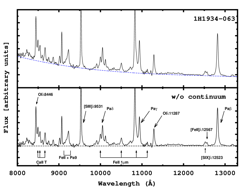
Figure 1.— Example of continuum subtraction and the most relevant emission lines used in this work. Top Panel: Observed Spectrum of 1H 1934-063 (in the rest frame) and the continuum fit (blue dashed line). Bottom Panel: Spectrum of 1H 1934-063 without the continuum. The black arrows point to the most relevant lines for this paper. The dashed black line indicates the zero continuum level.

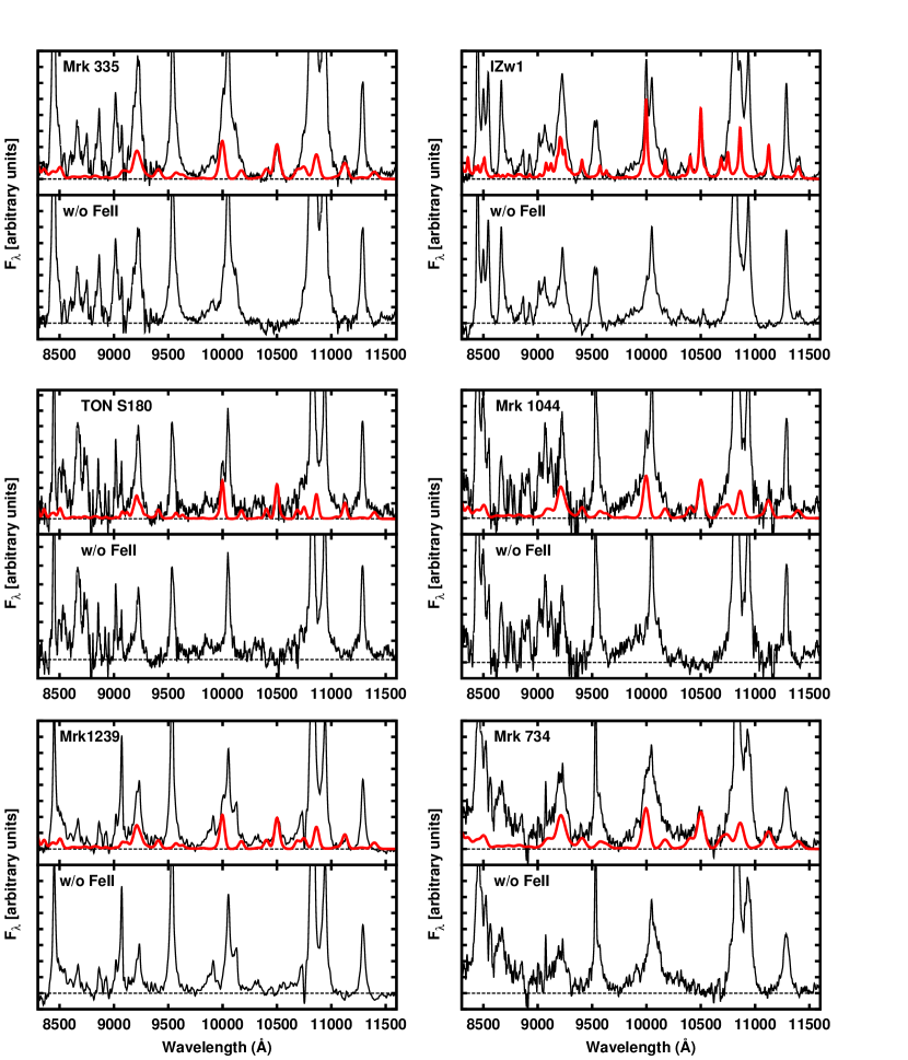
Figure 2.— Top panels: continuum-subtracted spectrum (in the rest frame) of each object of the sample (black line), with the spectrum of Fe ii calculated from the semi-empirical template (in bold) superposed. Bottom: spectrum of each object of the sample without this contribution.

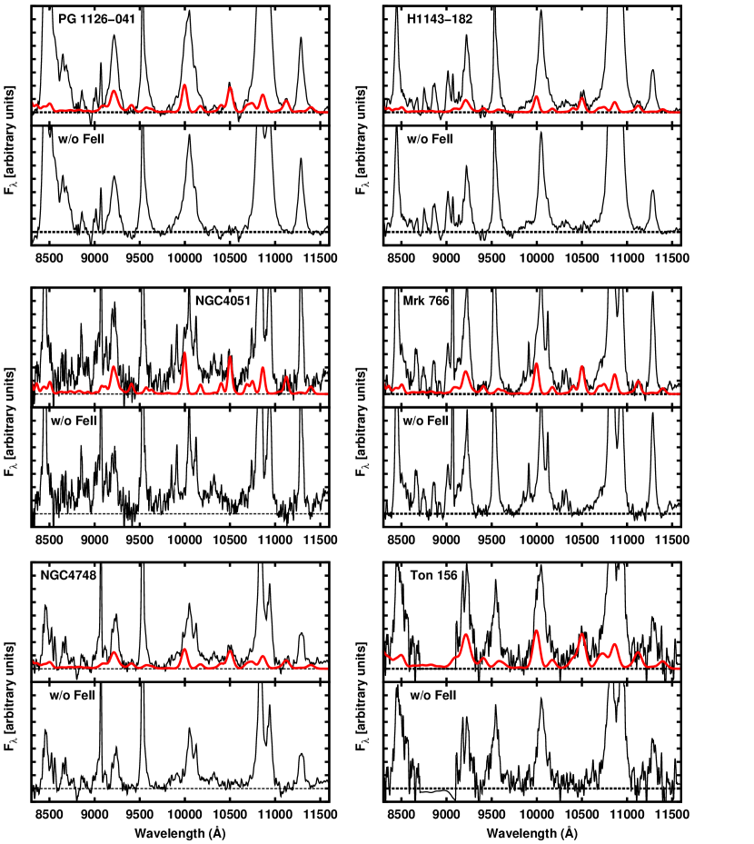
Figure 3.— Continuation of Figure 2

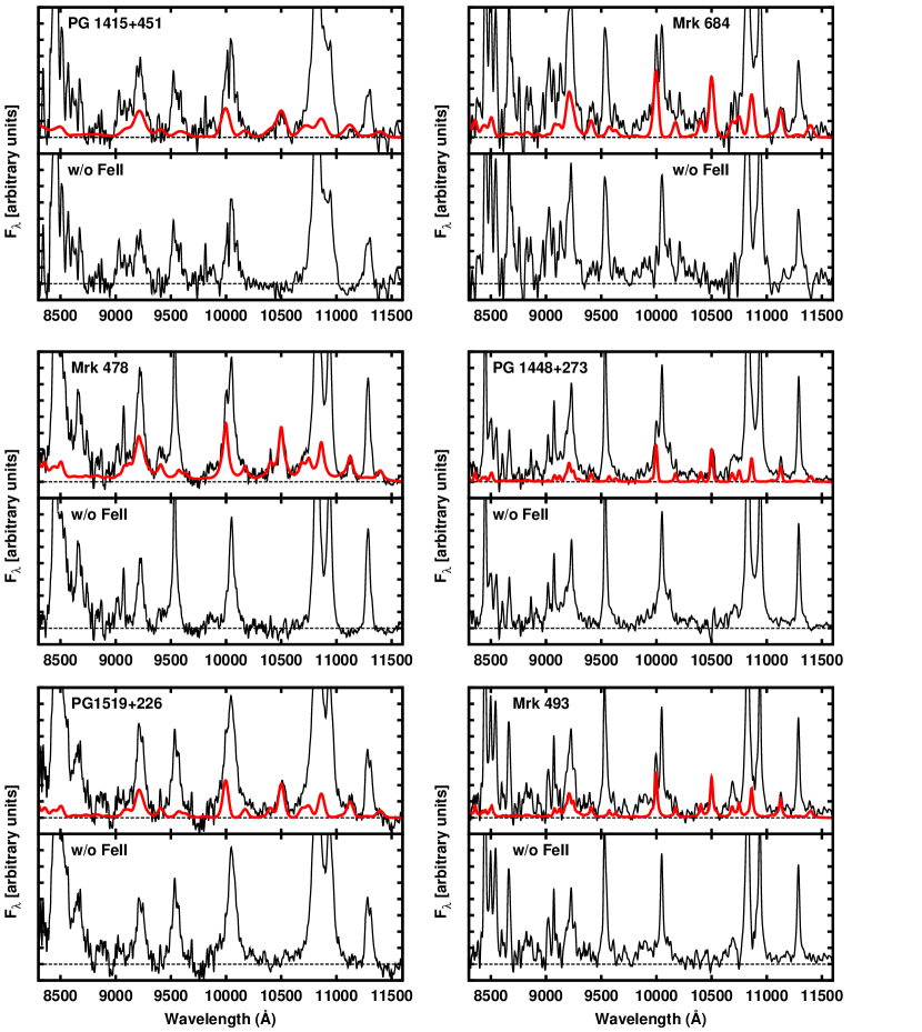
Figure 4.— Continuation of Figure 2

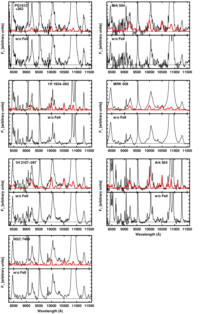
Figure 5.— Continuation of Figure 2

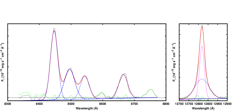
Figure 6.— Example of line deblending for 1H 1934-063. The left panel shows each line of the Ca ii triplet (blue dotted-dashed line), the O i $\lambda$8446 line (blue dotted line) and the total fit of these lines (red dashed line). Right panel shows the deblend of the Pa$\beta$ line in broad (two-dotted blue line) and narrow (dotted-dashed magenta line) components. The red dashed line is the sum of these two components.

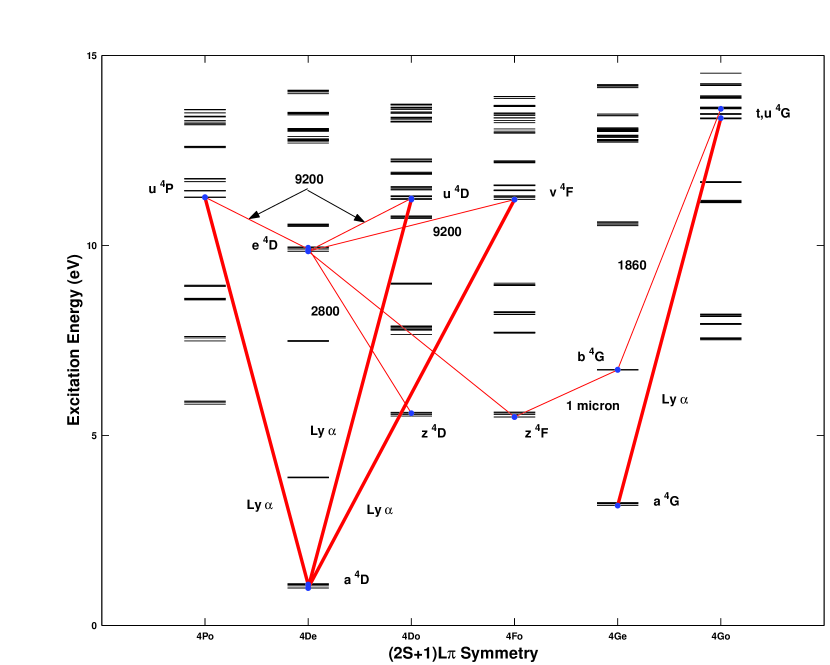
Figure 7.— Partial Grotrian diagram for the Fe ii system showing the transitions forming the 1 $\mu$m lines and the bump at 9200 Å. The Ly$\alpha$ fluorescence route and the subsequent cascades. The 1 $\mu$m lines are produced by the multiplets transitions b⁴G$\rightarrow$z(⁴F, ⁴D). The Fe ii $\lambda$9200 bump is produced by the transitions u(⁴P,⁴D),v⁴F$\rightarrow$e⁴D. Figure from Sigut $\&$ Pradhan (2003)

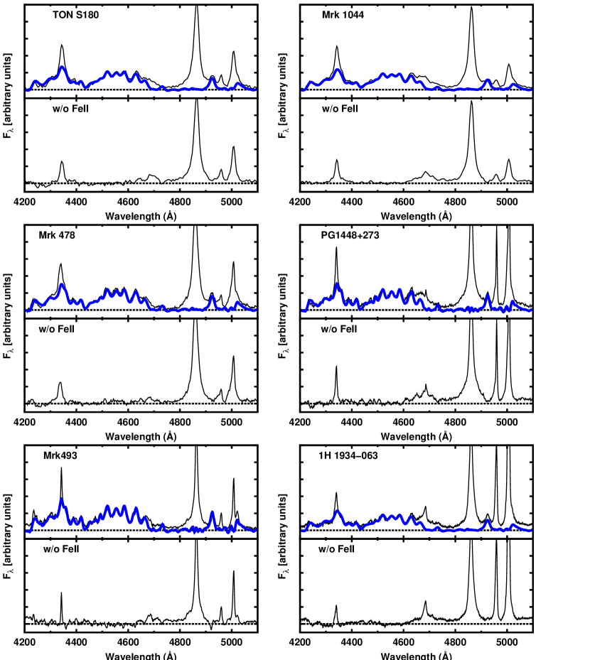
Figure 8.— Examples of The convolved optical Fe ii template. Top panels show the continuum-subtracted spectrum of the AGN (black line), with the optical spectrum of Fe ii (blue bold line) superposed. Bottom panels show the spectrum of each object without this emission.

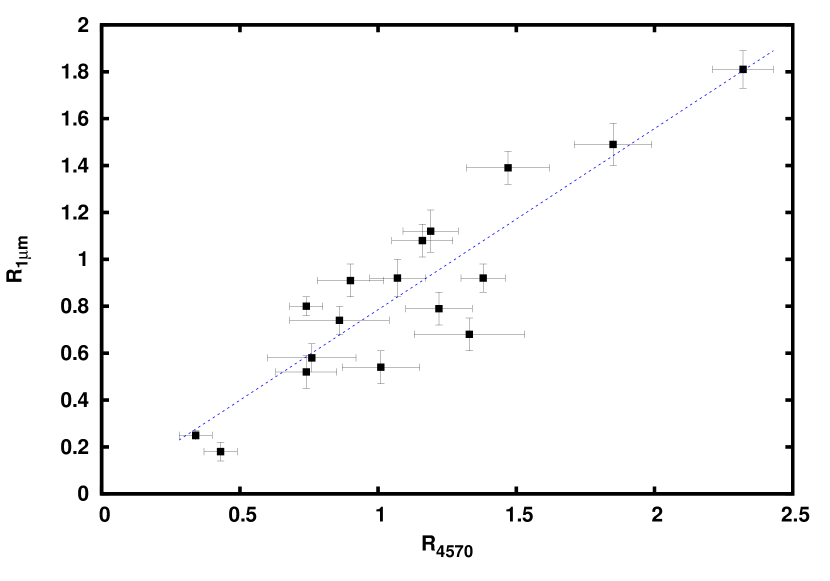
Figure 9.— Correlation between R_1μm and R₄₅₇₀. The blue dotted line shows the best linear fit.

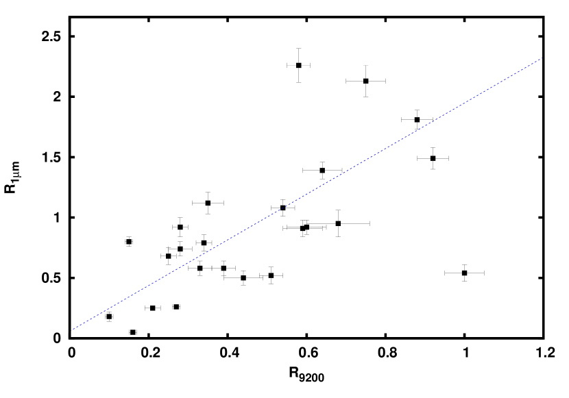
Figure 10.— Correlation between R_1μm and R₉₂₀₀. The blue dotted line shows the best linear fit.

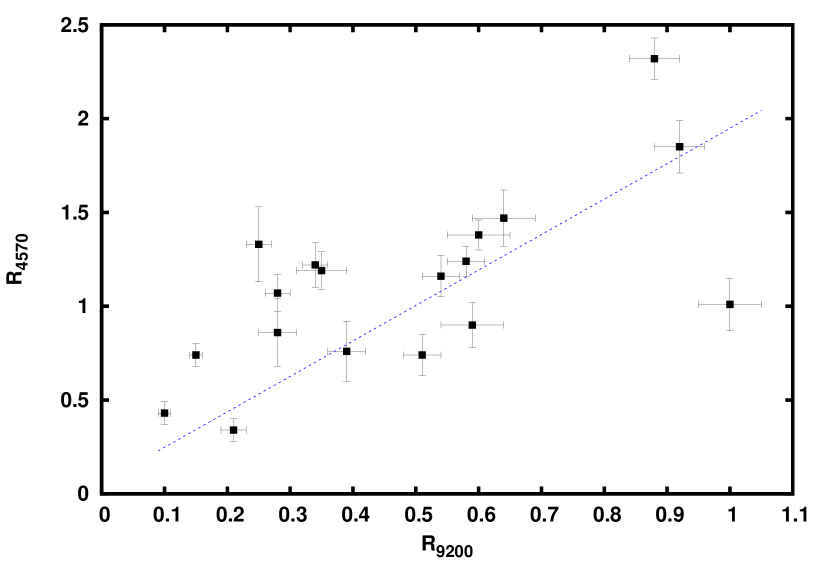
Figure 11.— Correlation between R₉₂₀₀ and R₄₅₇₀. The blue dotted line shows the best linear fit.

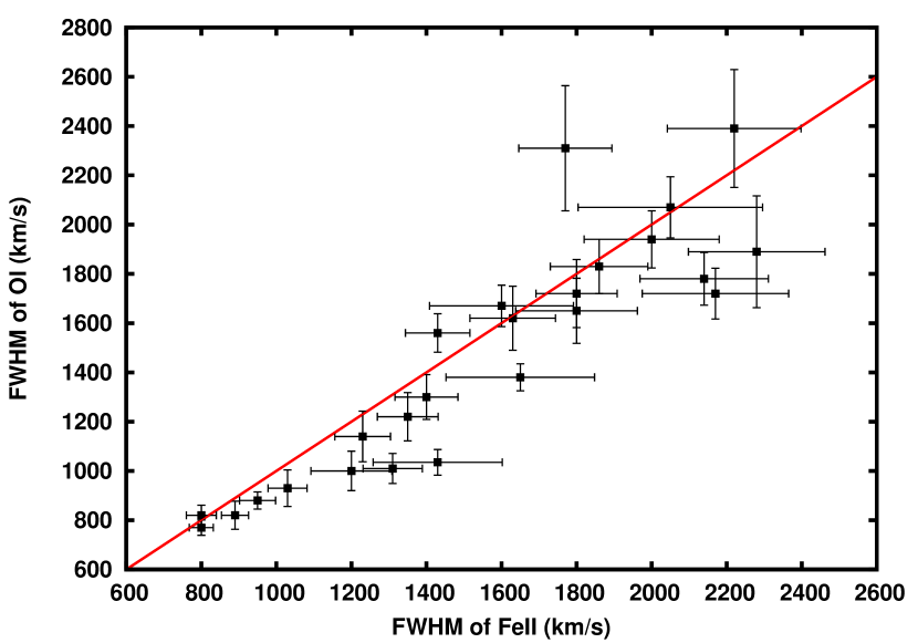
Figure 12.— Correlation between the FWHM of Fe ii and the FWHM of O i. The red line shows the unitary relationship.

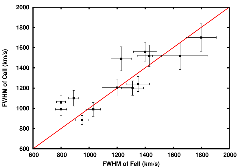
Figure 13.— Correlation between the FWHM of Fe ii and the FWHM of Ca ii. The red line shows the unitary relationship.

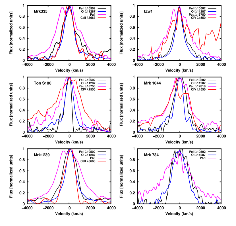
Figure 14.— Comparison between the broad line profiles for the most important lines in this work for each object of the sample: Fe ii (black line), O i (blue line) and Pa$\beta$ (magenta line). The C iv (red line) was added for the objects in which it was available in order to have a high ionization line to compare. In all cases, the lines were normalized to their peak intensity and Pa$\beta$ had its narrow component removed according to the procedure described in Section 3.

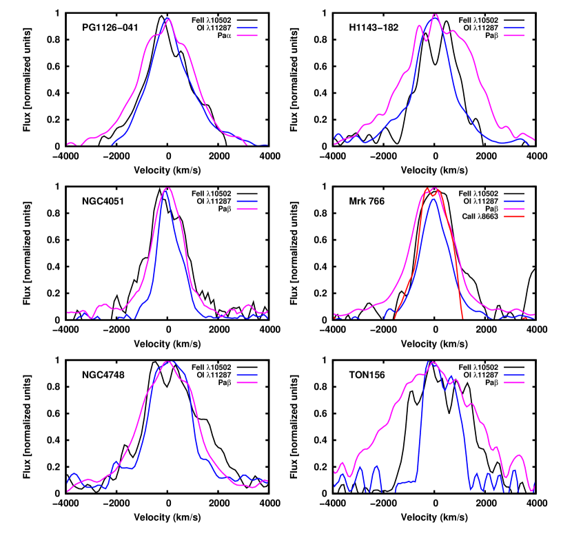
Figure 15.— Continuation of Figure 14

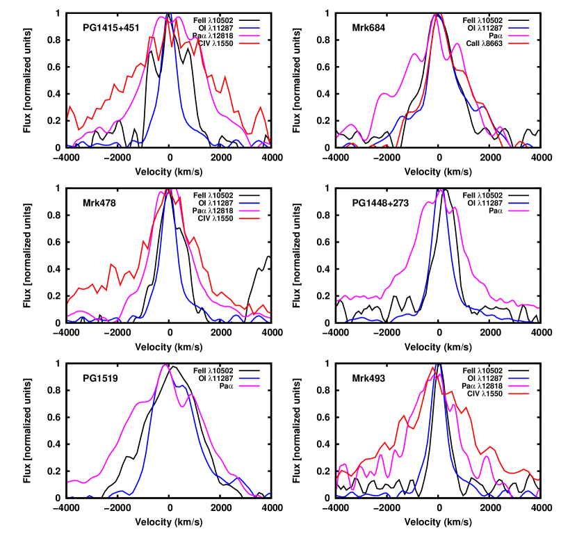
Figure 16.— Continuation of Figure 14

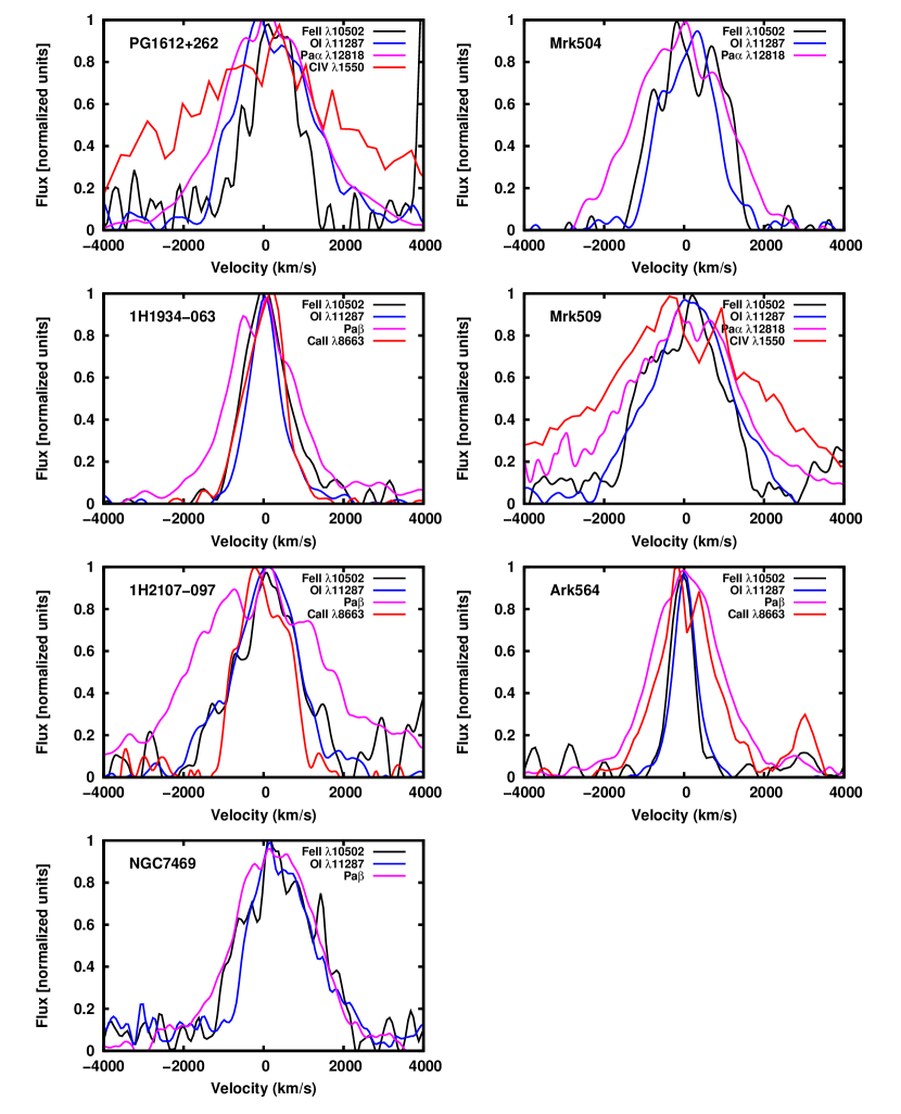
Figure 17.— Continuation of Figure 14

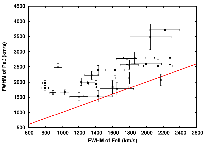
Figure 18.— Correlation between the FWHM of Fe ii and the FWHM of Pa$\beta$. The red line shows the unitary relationship.

References

- Baldwin et al (2004) Baldwin, J. A., Ferland, G. J., Korista, K. T., Hamann, F., LaCluyzé, A. 2004, ApJ, 615,610
- Barth et al. (2013) Barth, A. J., Pancoast, A., Bennert, V. N., et al., 2013, ApJ, 769, 128
- Beers et al. (1990) Beers, T. C., Flynn, K. Gebhardt, K. 1990, AJ, 100,32
- Bischoff Kollatschny (1999) Bischoff, K.; Kollatschny, W. 1999, A&A, 345, 49
- Boroson Green (1992) Boroson T. A., Green, R. F. 1992, ApJS, 80, 109
- Bruhweiler Verner (2008) Bruhweiler, F., Verner, E. 2008, ApJ, 675, 83
- Cushing et al. (2004) Cushing, M., Vacca, W. D., Rayner, J. T. 2004, PASP, 116, 362
- Dietrich et al. (1993) Dietrich, M.; Kollatschny, W.; Peterson, B. M., et al. 1993, ApJ, 408, 416
- Dong et al. (2010) Dong. X-B, Ho, L. C., Wang, J-G, Wang, T-G., Wang, H., Fan, X. Zhou, H. 2010, ApJS, 721, 123
- Dong et al. (2011) Dong. X-B, Wang, J-G, C. Ho, L. C., Wang, T-G., Fan, X., Wang, H., Zhou, H. Yuan, W. 2011, ApJ, 736, 86
- Garcia-Rissmann et al. (2012) Garcia-Rissmann, A., Rodríguez-Ardila, A., Sigut, T. A. A., Pradhan, A. K. 2012, ApJ, 751, 7
- Gaskell (2009) Gaskell, C. M. 2009, New A Rev., 53, 140
- Giannuzzo Stirpe (1996) Giannuzzo, E. M. Stirpe, G. M. 1996, A&A
- Hu et al. (2008) Hu, C., Wang, J.-M, Ho, L C., Chen, Y.-M., Zhang, H.-T., Bian, W.-H., Xue, S.-J. 2008, ApJ, 687, 78
- Hu et al. (2015) Hu, C., Du, P., Li, Y-R, Wang, F., Qu, J., Bai, J-M., Kaspi, S., Ho., L. C., Netzer, H. Wang, J-M. 2015, ApJ, 804, 138
- Joly (1991) Joly, M., 1991, A&A, 242, 49
- Joly (1993) Joly, M., 1993, Ann. Phys. Fr., 18, 241
- Kaspi et al. (2000) Kaspi, S., Smith, P.l S., Netzer, H., et al. 2000, ApJ, 533, 631
- Kollatschny et al. (1981) Kollatschny, W.; Fricke, K. J.; Schleicher, H.; Yorke, H. W. 1981, A&A, 102, 23
- Kollatschny Fricke (1985) Kollatschny, W.; Fricke, K. J. 1985, A&A, 146, 11
- Kollatschny Dietrich (1996) Kollatschny, W.; Dietrich, M. 1996, A&A, 314, 43
- Kollatschny et al. (2000) Kollatschny, W., Bischoff, K. Dietrich, M. 2000, A&A, 361, 901
- Kollatschny et al. (2006) Kollatschny, W., Zetzl, M. Dietrich, M. 2006, A&A, 454, 459
- Kovačević et al. (2010) Kovačević, J., Popović, L. Č., Dimitrijević, M. S. 2010, ApJS, 673, 69
- Kuehn et al. (2008) Kuehn, C. A., Baldwin, J. A., Peteron, B.M., Korista, K. T. 2008, ApJ, 673, 69
- Landt et al. (2008) Landt, H., Bentz, M. C., Ward, M. J., Elvis, M., Peterson, B. M., Korista, K. T., Karovska, M. 2008, ApJS, 174, 282
- Laor Baskin (2005) Baskin, A., Laor, A. 2005, MNRAS, 356, 1029
- Lawrence et al. (1997) Lawrence, A., Elvis, M., Wilkes, B. J., McHardy, I., Brandt, N. 1997, MNRAS, 285, 879
- Martínez-Aldama et al. (2015) Martínez-Aldama, M. L., Dultzin, D., Marziani, P., Sulentic, J. W., Bressan, A., Chen, Y., Stirpe, G. M. 2015, ApJ, 217, 3
- Matsuoka et al. (2007) Matsuoka, Y., Oyabu, S., Tsuzuki, Y., Kawara, K. 2007, ApJ, 663, 781
- Matsuoka et al. (2008) Matsuoka, U., Oyabu, S., Tsuzuki, Y., Kawara, K. 2008, ApJ, 673, 62
- North et al. (2006) North, M., Knigge, C. Goad, M. 2006, MNRAS, 365, 1057
- Osterbrock (1989) Osterbrock, D. E. 1989, University Science Books, v. 422
- Penston (1987) Penston, M. V. 1987, MNRAS, 229, IP
- Persson (1988) Persson, S. E. 1988, ApJ, 330, 751
- Peterson et al. (1998) Peterson, B. M., Wanders, I., Bertram, R., et al. 1998, ApJ, 501, 82
- Peterson et al. (2004) Peterson, B. M., Ferrarese, L., Gilbert, K. M., et al. 2004, ApJ, 613, 682
- Peterson Wandel (1999) Peterson, B., Wandel, A. 1999, ApJ, 521, L95
- Pogge Owen (1993) Pogge, R. W., Owen, J. M. 1993, Ohio State Univ. Int. Rep. 93-01
- Popović et al. (2007) Popović, L. Č., Smirnova, A., Ilic, D., Moiseev, A., Kovačević, J., Afanasiev, V. 2007, in The Central Engine of Active Galactic Nuclei, ed. L. C. Ho J.-M. Wang (San Fracisco: ASP), 552
- Pradhan Nahar (2011) Pradhan A. K. Nahar S. N., 2011, Atomic Astrophysics and Spectroscopy. Cambridge Univ. Press, Cambridge
- Rayner et al. (2003) Rayner, J. T., Toomey, D. W., Onaka, P. M., et al. 2003, PASP, 115, 362
- Riffel et al. (2006) Riffel, R., Rodrí́guez-Ardila, A., Pastoriza, M. 2006, A&A, 457, 61
- Rodríguez-Ardila et al. (2000) Rodríguez-Ardila, A., Binette, L., Pastoriza, M. G., Donzelli, C. J. 2000a, ApJ, 538, 581
- Rodríguez-Ardila et al. (2002) Rodríguez-Ardila, A., Viegas, S. M., Pastoriza, M. G., Prato, L. 2002, ApJ, 565, 140
- Rudy et al. (2000) Rudy, R. J., Mazuk, S., Puetter, R. C., Hamann, F. 2000, ApJ, 539, 166
- Sargent (1968) Sargent W. L. W. 1968, ApJ, 152, 31
- Schlegel et al. (1998) Schlegel, D. J., Finkbeiner, D. P., Davis, M. 1998, ApJ, 500, 525
- Shapovalova et al. (2012) Shapovalova, A. I., Popovic, L. C., Burenkov, A. N., et al. 2012, ApJS, 202, 22
- Sigut Pradhan (1998) Sigut, T. A. A., Pradhan, A. K. 1998, ApJ, 499, L139
- Sigut Pradhan (2003) Sigut, T. A. A., Pradhan, A. K. 2003, ApJS, 145, 15
- Sigut et al. (2004) Sigut, T. A. A., Nahar, S. N., Pradhan, A. K. 2004, ApJ, 611, 81
- Sluse et al. (2007) Sluse, D., Claeskens, J.-F., Hutsemémers, D., Surdej, J. 2007, A&A, 468, 885.
- Sulentic et al. (2000) Sulentic, J. W., Zwitter, T., Marziani, P., Dultzin-Hacyan, D. 2000, ApJ, 536, L5
- Tsuzuki et al. (2006) Tsuzuki, Y., Kawara, K., Yoshii, Y., et al. 2006, ApJ, 650, 57
- Vacca et al. (2003) Vacca, W. D., Cushing, M. C., Rayner, J. T. 2003, PASP, 115, 389
- Verner et al. (1999) Verner, E. M., Verner, D. A., Korista, K. T., Ferguson, J. W., Hamann, F. Ferland, G. J. 1999, ApJ, 120, 101
- Véron-Cetty et al. (2004) Véron-Cetty, M.-P., Joly, M., Véron, P. 2004, A&A, 417, 515
- Vestergaard Wilkes (2001) Vestergaard, M., Wilkes, B. J. 2001, ApJS, 134, 1
- Wang et al. (2005) Wang, J., Wei, J. Y. He, X. T. A&A, 436, 416
- Wills et al. (1985) Wills, B. J., Netzer, H., Wills, D. 1985, ApJ, 288, 94
- Wampler Oke (1967) Wampler, E. J. Oke J. B. 1967, ApJ, 148, 69