Measuring Light Echos in NGC 4051

Abstract

Five archived X-ray observations of NGC 4051, taken using the NuSTAR observatory, have been analysed, revealing lags between flux variations in bands covering a wide range of X-ray photon energy. In all pairs of bands compared, the harder band consistently lags the softer band by at least 1000 s, at temporal frequencies $\sim 5\times 10^{-5}$ Hz. In addition, soft-band lags up to 400 s are measured at frequencies $\sim 2\times 10^{-4}$ Hz. Light echos from an excess of soft band emission in the inner accretion disk cannot explain the lags in these data, as they are seen in cross-correlations with energy bands where the softer band is expected to have no contribution from reflection. The basic properties of the time delays have been parameterised by fitting a top hat response function that varies with photon energy, taking fully into account the covariance between measured time lag values. The low-frequency hard-band lags and the transition to soft-band lags are consistent with time lags arising as reverberation delays from circumnuclear scattering of X-rays, although greater model complexity is required to explain the entire spectrum of lags. The scattered fraction increases with increasing photon energy as expected, and the scattered fraction is high, indicating the reprocessor to have a global covering fraction $\sim 50\%$ around the continuum source. Circumnuclear material, possibly associated with a disk wind at a few hundred gravitational radii from the primary X-ray source, may provide suitable reprocessing.

1 Introduction

Variations in X-ray flux are common in Active Galactic Nuclei (AGN), where factors of several change are evident over all timescales observed, i.e. from tens of seconds to years. Interpretation of the flux variations and the dependences on photon energy may allow insight into the physical processes that are important in the immediate neighborhood of the supermassive nuclear black hole. Construction of a power spectral density (PSD) can help characterize the variations, showing the relative importance of the different temporal modes sampled by the data, while the lag spectrum shows the time lags between two light curves extracted from different energy ranges; these are analyzed as a function of the frequency of Fourier modes (convention defines a positive lag as hard photons lagging soft).

Time delays are expected to arise from reverberation in the X-ray band, caused by reprocessing and scattering of the continuum radiation by circumnuclear material. Of particular interest is the so-called transfer function, that is a measure of the time delays between time series constructed in differing bands of X-ray photon energy, analyzed as a function of the temporal frequency of modes of variation. Energy- and frequency-dependent time delays appear to be a common feature of the X-ray emission from AGN (e.g. De Marco et al., 2013).

There are currently two principal mechanisms that have been invoked in the literature to explain time delays between X-ray energy bands. The first of these is time delays that may be associated with the possible inwards propagation of fluctuations on the accretion disk (e.g. Kotov et al., 2001; Arévalo et al., 2006). The inner accretion disk is thought to be hotter than the outer disk, so a delayed fluctuation arriving at the inner disk may stimulate harder X-ray emission than would be produced at larger radii, leading to an energy-dependent time delay of hard photon flux variations lagging soft photon flux variations. However, while this model may work well for X-ray binaries with their hotter accretion disks, in AGN the observed X-ray emission is not thought to arise directly from the disk, as the disk should be too cool. Instead, it is commonly supposed that disk photons are Compton upscattered in energy in a hot corona, of unknown geometry (Haardt & Maraschi, 1991). However, in order to produce the observed powerlaw X-ray spectrum, the optical depth to Compton scattering must be sufficiently high that memory of the input spectrum is largely lost (Titarchuk, 1994) - thus it seems likely that this model needs to assert that coronal fluctuations may produce the require spectral-dependent time delays. It is also commonly supposed that the X-ray source is a compact region close to the black hole event horizon, in order to create a high equivalent width of strongly redshifted Fe K line emission (Miniutti & Fabian, 2004). However, if the coronal size is too small then there is no clear mechanism for the inwards disk fluctuations to be transferred into a change in the X-ray emission via the corona: the corona has to be extended in order for the inwards propagation model to work. Despite these difficulties, the ‘propagation of fluctuations’ model remains a popular choice in the literature (Uttley et al., 2014).

The second possible mechanism supposes that time delays arise from light travel time delays, arising when X-ray photons Compton scatter from circumnuclear material. Such a mechanism has been invoked to explain either short timescale delays in AGN (e.g. Fabian et al., 2009) or the entire transfer function of delays across all timescales (e.g. Miller et al., 2010a). These possibilities will be discussed later in this paper in the context of new observations of the nearby AGN NGC 4051.

In the context of reverberation models, the delayed signal, or “light echo” arises from scattering of the X-ray continuum from absorbing circumnuclear or accretion disk material - a process commonly known as ‘reflection’ in the case of optically-thick material. The reverberation component is expected to have a hard spectrum relative to the primary continuum and the contribution of reflection increases with energy. An observed time series generally comprises both direct emission and delayed, scattered emission, so that the net observed reverberation time delay is diluted according to the fraction of direct light that is present. In the harder energy bands the contribution of delayed emission increases and observed time lag tends towards an undiluted value (Miller et al., 2010a). Reverberation models predict we should see a strong delayed signal in the hard X-ray band, peaking above 10 keV.

Owing to low sensitivity, lack of spatial resolution and high background levels, there has been no mission prior to NuSTAR that has allowed useful reverberation analysis above 10 keV. Early results show the value of NuSTAR in X-ray reverberation analysis. Zoghbi et al. (2014) presented the first analysis of high-frequency time lags in NuSTAR data above 10 keV, showing the Compton hump to lag the continuum variations by 1–2 ks in MCG–5-23-16. Kara et al. (2015) claimed a similar result for SWIFT J2127.4+5654 and NGC 1365. Emission from around Fe K$\alpha$ was also found to lag the continuum in all three sources.

This work presents a study of the timing and spectroscopic properties of NGC 4051, observed in five NuSTAR observations. In Section 2 we discuss recent analyses of X-ray observations of NGC 4051. In Section 3, we describe the NuSTAR data reduction. In Section 4 we present the spectral analysis of the source. In Section 5 we describe our timing analysis methods and in Section 6 we discuss the results in the context of a light echo model for the X-ray reprocessor.

2 NGC 4051

NGC 4051 is a bright, nearby narrow-line Seyfert 1 AGN with low black hole mass, (M$\simeq 1.7\times 10^{6}{\rm M_{\odot}}$; Denney et al. 2010) and high accretion rate ($\sim 10$ % of Eddington), making it one of the most variable Seyfert galaxies in the X-ray band, with factors up to 15 observed on timescales of tens of ks (Ponti et al., 2006). The X-ray spectrum has been well studied and shows a multi-phase outflow, with zone velocities ranging from a few hundred to few thousand km/s, (Pounds et al., 2004a; Pounds & Vaughan, 2011). The ionization of some of the absorbing zones has been observed to change in response to the varying continuum (Lobban et al., 2011; Krongold et al., 2007). The strong and persistent reprocessing signatures show that there is a large amount of circumnuclear material in NGC 4051, making this an ideal target for a detailed reverberation study.

Outflowing reprocessor zones with velocities $50-400$ km s^-1 are also detected in UV spectroscopy of this source (Kaspi et al., 2004). These fit well into the Krongold et al. (2007) picture of an absorbing multi-phase wind and it may be that a significant part of the observed reflection comes from such a wind (Turner et al., 2007). The X-ray continuum itself varies by up to a factor 15 on timescales as short as 20 ks (Ponti et al., 2006). In its low state Ovii and Oviii emission lines from distant photoionized gas are prominent (Pounds et al., 2004b; Ponti et al., 2006) and there is likely also a component of distant neutral reflection (Ponti et al., 2006). Ionised Fe x emission is also detected optically up to 150 pc from the central source (Nagao et al., 2000). In summary, the reprocessed spectrum for NGC 4051 appears to include contributions from the inner accretion disk, the broad-line region and from more distant dusty regions of circumnuclear gas.

To study the temporal behaviour of the X-ray emission, McHardy et al. (2004) combined 6.5 years of observations by RXTE with a long observation by XMM-Newton (hereafter XMM), finding the lag of hard X-ray fluctuations to increase and coherence to decrease as band separation increases. They also found the lag and coherence to be greater for variations of longer time period. This behaviour suggested higher photon energies and shorter variability timescales to be associated with smaller radii.

Miller et al. (2010a) presented two long Suzaku exposures of NGC 4051, finding a strong hard component above 10 keV, some fraction of which varies with the power-law continuum. The power spectrum was non-stationary, showing differences between the low and high flux states. This was confirmed in XMM observations by Alston et al. (2013), who also measured negative time lags and found that the shape of the lag spectra depends on source flux. Frequency-dependent positive time lags $970\pm 225$ s were measured by Miller et al. (2010a) and suggested to be explained by the effects of reverberation in the hard band, caused by reflection from a thick shell of material with maximum lags of about 10,000s. The reflecting material must extend to a distance of about $1.5\times 10^{14}{\rm cm}$, i.e. 600 gravitational radii from the illuminating source with high global covering factor ($C_{g}>0.44$). The reflection may occur from Compton thick parts of the disk wind, seen out of the line-of-sight. These very long lags in the hard band also exclude the possibility that the hard component originates as reflection from the inner accretion disk in NGC 4051 Miller et al. (2010a).

3 Analysis of the NuSTAR data

Table 1: Observation Log

Date	Observation	Exposure	ct/s	ct/s	flux	flux
			2-10 keV	10-50 keV	2-10 keV	10-50 keV
2013-06-17 16:41:07	60001050002	9.4	0.25	0.11	1.99	3.79
2013-06-17 21:21:07	60001050003	45.7	0.25	0.11	1.80	3.17
2013-10-09 13:41:07	60001050005	10.2	0.19	0.09	1.31	2.89
2013-10-09 20:01:07	60001050006	49.6	0.13	0.07	0.93	2.29
2014-02-16 13:36:07	60001050008	56.7	0.35	0.13	2.99	4.19

.

NuSTAR observed NGC 4051 during five observations spread over 2015 May 15 – 22, with exposure times between 9.4 – 56.7 ks (Table 1). The data from both focal plane modules (FPMA and FPMB) and for all observations were reprocessed and cleaned using the most recent version of the NuSTAR pipeline (within HEASOFTv16.6) and calibration files (CALDB version 20140715), resulting in 172 ks of good on-source exposure (Table 1).

We extracted spectra and light curves from a circular region of 30” radius, centered on the nucleus. Background spectra and light curves were extracted from two circular regions that are free of any obvious point sources and the ratio of source to background areas for the extraction cells was 1:5.5.

NGC 4051 shows strong X-ray variability across the observation set (Table 1 and Fig.  1). The background is 0.5-2% of the total counts in the 2-70 keV band, 2-5% in the 10-70 keV band. There is no concern regarding dead time in this count rate regime (Table 1).

Examination of the background-subtracted light curves reveals strong time variability within all of the observations (Fig  1). As observations 60001050002 and 60001050003 are very close in count rate and spectral shape and were taken close together in time, we combine those exposures into a single spectrum for the spectral analysis (Table 2).

The spectral data from those summed observations, plus spectra from the other three observations were fit for modules FPMA and FPMB simultaneously. The calibration offset recommended between those two instruments is in the range 0.95-1.05, and so a constant component was allowed in the model, linked to be a single floating value that we fit to obtain a cross-normalization constant 1.05 between the two FPM instruments.

4 Spectral fitting

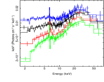
Figure 1: NuSTAR data for NGC 4051 - for clarity, only FPMA data are shown. Spectral variability is dominated by changes in the continuum level that drive lagged changes in scattered light. Observations correspond to the colored lines as: 02$+03$ (black), 05 (red), 06 (green) and 08 (blue) – see Table 2

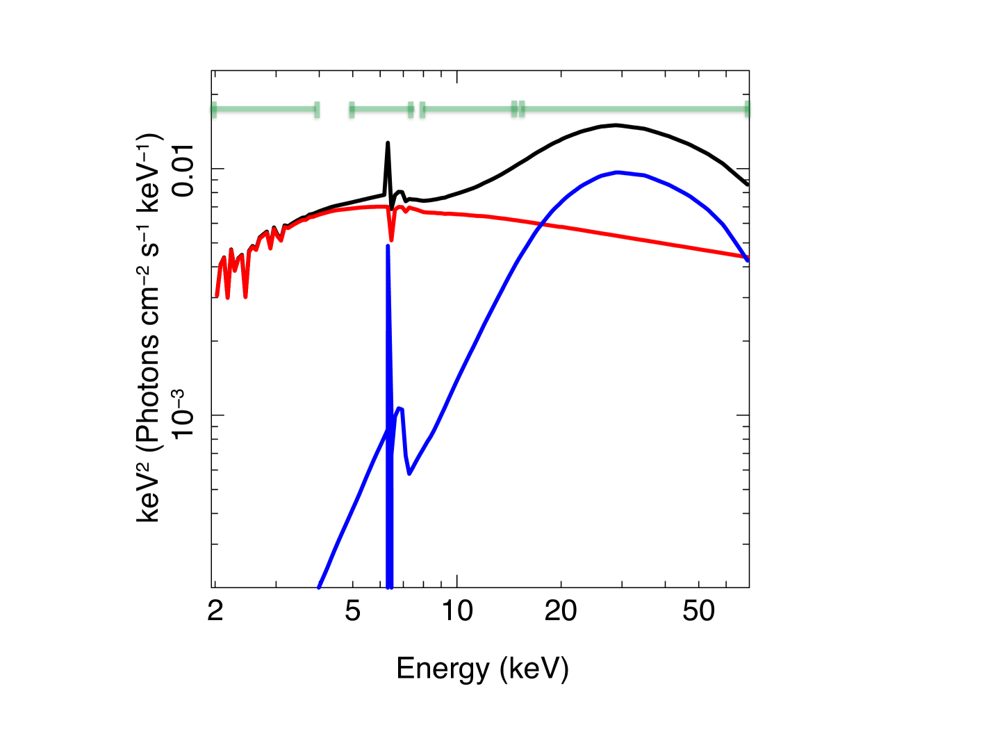
Figure 2: The mean model for NGC 4051 with the boundaries shown for the bands chosen for timing analysis shown as green horizontal lines. The mean powerlaw component is shown in red, the mean scattered component is shown in blue. Both components are modified by a layer of ionized gas and the summed model is shown as a black line.

Table 2: Reprocessing Model

Observation	${\rm N_{H}}^{1}$	N${}_{\rm PL}^{2}$	N${}_{\rm Sc}^{3}$	F${}_{\rm Fe}^{4}$	EWFe
02$+$03	4.75${}^{+1.25}_{-1.19}$	$12.31\pm 0.9$	$7.06\pm 0.15$	2.78$\pm 0.74$	144
05	6.28${}^{+2.12}_{-2.50}$	$7.84\pm 0.66$	$6.72\pm 0.15$	$4.82\pm 0.11$	347
06	12.75${}^{+1.95}_{-4.11}$	6.91$\pm 0.52$	$5.05\pm 0.10$	1.67$\pm 0.65$	191
08	2.70${}^{+0.80}_{-0.70}$	17.33 $\pm 1.17$	$6.86\pm 0.15$	3.58$\pm 0.75$	125

To remain within the well-calibrated regime for NuSTAR, this paper restricts consideration of spectral data to the $\sim$2 - 70 keV band. We rebin the spectral data first to 1024 channels to reduce the spectral oversampling, then apply a grouping to achieve a minimum of 20 photons per energy channel in order to facilitate the use of $\chi^{2}$ statistics. Models were fit to the data using the software package xspec ver. 12.9.0 (Arnaud 1996). All models included the Galactic line-of-sight absorption, N${}_{\rm H,Gal}=1.35\times 10^{20}{\rm cm}^{-2}$ (Dickey & Lockman, 1990), although this had a negligible effect on the fit parameters owing to the spectral cut-off being relatively high, at 2 keV. All model components were adjusted to be at the redshift of the host galaxy, except for the Galactic absorption. In the following, unless otherwise stated, fit parameters are quoted in the rest-frame of the source and errors are at the 90% confidence level for one interesting parameter ($\Delta\chi^{2}=2.706$).

Initial inspection of the data revealed the source to be flatter in the low flux states, and steeper in the high states, as observed previously (Miller et al., 2010a). Based upon this, and the previous modeling of the source (Miller et al., 2010a; Lobban et al., 2011) we adopted a simple model of a power law continuum plus neutral scattering gas, all covered with an ionized absorber plus the Galactic column density of neutral gas.

While the ionized absorber is known to be complex and multi-zoned, the lack of soft-band data, and modest spectral resolution of these data prevented us from creating a sophisticated model of that absorbing gas. It was found that a single ionized gas zone was adequate to model the low energy behavior of the source. Thus we fit the $2.0-70.0$ keV data using a model composed of a power-law continuum, modified by passage through a uniform sphere of ionized gas characterized by an xstar model table. For the ionized absorber table we used version 2.1ln11 of the xstar code (Kallman & Bautista, 2001; Kallman et al., 2004), assuming the abundances of Grevesse & Sauval (1998). xstar models the absorbing gas as thin slabs, with parameters of atomic column density and ionization parameter $\xi$, defined as

$$\xi=\frac{L_{\rm ion}}{nR^{2}}$$

that has units erg cm s^-1 and where $L_{\rm ion}$ is the ionizing luminosity between 1 and 1000 Rydbergs, $n$ is the gas density in cm^-3 and $R$ is the radial distance (cm) of the absorbing gas from the central continuum source. The spectral energy distribution was taken to be a simple power law with $\Gamma=2.5$. Following Lobban et al. (2011) the turbulent velocity was taken as $\sigma=200$ km s^-1.

The neutral scattering reprocessor gas was modeled using the toroidal reprocessor model, MYTorus (Murphy & Yaqoob, 2009; Yaqoob et al., 2010). The torus has a circular cross section, whose diameter is characterized by the equatorial column density, ${\rm N_{H}}$. The torus is illuminated by a central X-ray continuum. The torus is assumed to have an opening angle (half angle) of 60^o, and this corresponds to a global covering factor of 50% (and a solid angle subtended by the structure at the central X-ray source of 2$\pi$ steradians). The MYTorus model self-consistently calculates the Fe K$\alpha$ and Fe K$\beta$ fluorescent emission lines in a separate table to the opacity profile and the scattered spectrum. The availability of these components of reprocessing in separate tables allows the use of the so-called “decoupled mode”, whereby one can allow the scattered, line emission and opacity tables to vary independently, to allow for time delays between direct continuum, Compton-scattered continuum, and fluorescent line photons. All tables include the effects of Compton scattering. The element abundances for MYTorus are solar (Anders & Grevesse, 1989) and the photoelectric absorption cross-sections are those of Verner et al. (1996). Our model included only the scattered spectrum and line emission component. Our fits assumed an inclination angle of 0^o for MYTorus, representative of a face-on scattering torus, with the reprocessing matter out of the direct line-of-sight.

This simple model provided a good fit to all of the flux states exhibited by NGC 4051 (Fig. 1, Table 2). The neutral scattering gas yielded column density ${\rm N_{H}}=6.0\pm 3.1\times 10^{24}{\rm cm^{-2}}$: with our model construction, this column density is that inferred for the scatterer only and not associated with the direct transmitted continuum. The emission line component of MYTorus has been converted to Fe K$\alpha$ line fluxes and equivalent widths for ease of interpretation of the tabulated fits.

The data are consistent with a constant column density for the scattering gas, and column variations for the ionized absorber such that in the high state, the column of the ionized gas is low. Other variations, such as the ionization state or covering fraction of the absorber cannot be ruled out using these data, so our fits provide only a simple parameterization of that aspect of the source behavior.

Fitting all the NuSTAR spectra simultaneously with a single spectral model (ie not allowing any spectral variation between epochs, so we could obtain the mean scattering fractions), we found the scattered X-ray component (including Fe K line) provides a fraction (of scattered to total flux in each band) $<0.14$, 0.17$\pm 0.08$, 0.25$\pm 0.08$ and 0.55 $\pm 0.10$ of the total flux in the 2-4.0, 5.0-7.5, 8-15 and 15-70 keV bands, respectively. The mean spectral model is shown in Fig. 2.

4.1 Alternative Models

It is instructive to explore parameter space for reflection models, as inner disk reflection has been invoked previously to explain the presence of negative lags in AGN lag spectra. To this end, we adopted the xilver model, that represents reflection from Compton Thick gas with fitable ionization parameter (García et al., 2013). Initially, we fit the spectra using xilver plus a continuum powerlaw, allowing a layer of neutral absorption, fixed to account for the Galactic column as in the previous fits. In the fit, the Fe abundance was fixed at the solar value, and the ionization parameter was allowed to be free. The fit allowed the relative fractions of each of these components to vary between flux states. This fit resulted in $\chi^{2}_{r}=1.18$ for 504 degrees of freedom. The photon index was $\Gamma=2.19\pm 0.03$, with ionization parameter $\xi=1.11\pm 0.02$. The reflection fraction was 7% in the 2 - 4 keV band, 23% in 5 - 7.5 keV, 31% in 8 - 15 keV and 52% in the 15-70 keV band and the uncertainties on all bands were $\sim 20\%$. Next we allowed the Fe abundance to be free, and then convolved an unconstrained kdblur kernel, to account for relativistic blurring. Neither of these additional freedoms resulted a significant change in the reflection fractions, the soft-band fraction is mostly constrained by the hardness of the spectrum.

5 Measurement of the X-ray Time-delay Transfer Function

To measure time delays between bands of differing photon energy, we adopt an extension of the method described by Miller et al. (2010a, b). In that method, time series in two broad bands of photon energy were created, then a maximum likelihood method was used to fit a joint model to the power spectral density (PSD) in the two bands and to the cross-spectral density, fitting to the data autocorrelation in the time domain. Time delays as a function of temporal frequency were obtained from the phases of the cross-spectral density. The method rigorously accounted for gaps in the timing data and allowed accurate estimates of statistical uncertainties in PSD, cross-spectral density and time delays, including estimation of the covariance between the measured time lag values if required. The method has been independently coded and tested by (Zoghbi et al., 2013).

In this paper, given the very broad bandpass afforded by the NuSTAR observations, we wish to measure the time delays between four energy bands: 2–4 keV, 5–7.5 keV, 8–15 keV, 15–70 keV. In section 6 we consider simple models that are jointly fitted to the time lags between pairs of these bands, and for that process to be statistically rigorous we need to estimate the full covariance matrix, not only between the time lag values in each lag spectrum, but also between the lag spectra of each pair of energy bands: because energy bands are in common between the possible combinations of pairings they are correlated. To measure the covariance, the Miller et al. (2010a, b) analysis was extended to jointly fit to three energy bands, thus obtaining the lag spectra of three possible pairs of energy bands (i.e. the lags between bands 1 & 2, between 2 & 3 and between 1 & 3, out of 3 bands) and the covariance matrix. Despite other studies in the literature also carrying joint analysis of multiple bands (e.g. Kara et al., 2015), no previous study has taken into account the covariance between the measurements: those studies are therefore not able to evaluate the statistical significance of any lag spectral features that may be found simply from inspection of either plotted points with error bars or from goodness-of-fit statistics - either of those approaches should require the full covariance to be included.

In this analysis, Fourier bandpowers of frequency width $\Delta\log_{10}\nu=0.2$ were evaluated. Each observed photon in the energy bands was given equal weight, such that, in the absence of significant background flux, the optimum signal-to-noise ratio was obtained, irrespective of the source spectrum or the instrument spectral response. Note that, although the best available photon calibration has been applied, inaccuracies in photon energy calibration have little effect on the results in these broad energy bands, and the analysis did not make use of knowledge of the instrument’s spectral response. However, the source spectrum and the instrumental spectral response should be considered when interpreting the results (for example, although the highest energy band extends to 70 keV, the results are completely dominated by photons from the lower end of the bandpass around 15 keV).

Owing to the complexity of joint fitting to multiple energy bands, our analysis can currently only be carried out on three simultaneous energy bands, which leads to the generation of three, correlated lag spectra. In our discussion, we concentrate on the three bands $2-4$ keV, $8-15$ keV and $15-70$ keV, although we also consider the lag spectra that arise from joint analysis of the three bands $2-4$ keV, $5-7.5$ keV and $15-70$ keV, where the middle energy bands includes the region of Fe K emission and absorption.

The ‘lag spectra’ of time delays in all four possible pairs of bands are shown in Fig. 3. The points with error bars show the results from the data analysis, the solid curve depicts a simple model which will be described in section 6. The horizontal bars on each point show the range of temporal frequency covered, the vertical bars indicate the statistical uncertainty in the measured values. In these spectra, we follow the convention that a delay of the higher energy band with respect to the lower energy band has a positive sign. Thus in all pairs of energy bands, the harder band consistently lags the softer band at temporal frequencies around $5\times 10^{-5}$ Hz. The largest time delays have values around 1000 s, but some negative delays are also measured with amplitudes as large as 400 s. Note that lags that are consistent with zero, or with being slightly negative, are observed at the lowest frequencies in some combinations of energy bands, as found also in low states of NGC 4051 by Alston et al. (2013) and as seen in general in the study of De Marco et al. (2013). Note also the very sharp negative features visible in the upper two panels of Fig. 3, with some evidence for such a feature also in the third panel, at frequencies around $2-4\times 10^{-4}$ Hz.

Much attention in the literature has focussed on similar negative lag features, where the soft-band time variations lead the hard-band time variations in some range of frequency. Armed with the full covariance matrix, we have evaluated their statistical significance in these data as follows. Let us suppose that, where a negative lag value has been measured, the true lag value in fact is zero and the negative lag value arises purely from statistical noise (both photon shot noise and time series sampling variance). Then the statistical significance may be evaluated by measuring the change in $\chi^{2}$ that results when any negative values are forced to a value of zero, instead of being allowed to be free parameters in the maximisation of the bandpower likelihood. The change, $\Delta\chi^{2}$, may be evaluated using the covariance matrix:

$$\Delta\chi^{2}=\vec{\Delta\tau}^{T}C^{-1}\vec{\Delta\tau}\,,$$ (1)

where $\vec{\Delta\tau}$ is a vector of modified lag values, $\vec{\Delta\tau}^{T}$ is its transpose and $C^{-1}$ is the inverse covariance matrix. For positive lags, $\Delta\tau=0$, so they make no contribution to $\Delta\chi^{2}$. For negative lags, $\Delta\tau$ is set to the measured maximum-likelihood lag value, so that we measure the effect on $\chi^{2}$ of forcing these values to be zero. The statistical significance may then be evaluated from a table of $\chi^{2}$ with the number of degrees of freedom given by the number of “zeroed” lag values. We note that this test introduces some element of a posteriori statistics, as we only test the significance of values which have been selected by the experimenter. However, those values have been selected not on the basis of their apparent statistical significance, but rather simply on the sign of the lag value, irrespective of whether the amplitude of the lag value is large or small. Table 3 shows the frequency ranges over which negative lags are observed and their statistical significance, for cross-correlations between all the energy bands that have been considered. It should be noted that, although the covariance between frequency values has been taken into account, the values quoted for the various pairings of energy bands are not statistically independent. Negative lags appear to be significant in all cross-correlations with the hardest band ($15-70$ keV), and marginally significant also between the $5-7.5$ and $2-4$ keV bands. These negative lag features will be discussed further in section 6.

energy		2–4	5–7.5	8–15	15–70
/keV
2–4	$\Delta\chi^{2}/\nu$		$10.4/4$	$3.7/4$	$45.3/4$
	$p$		$0.034$	$0.45$	$3\times 10^{-9}$
5–7.5	$\Delta\chi^{2}/\nu$	0.25-0.61		n/m	$29.3/4$
	$p$				$7\times 10^{-6}$
8–15	$\Delta\chi^{2}/\nu$	0.15-0.39	n/m		$7.5/2$
	$p$				$0.024$
15–70		0.15-0.39	0.15-0.39	0.25-0.39

Table 3: Table of statistical significance of negative lag values, for combinations of pairs of energy bands used in the cross-correlation analysis. An entry of “n/m” indicates that lag spectrum was not measured. The lower left triangle shows the range of frequency over which a negative lag was observed, in units of mHz. The upper right triangle gives the $\Delta\chi^{2}$ value, the number of degrees of freedom, $\nu$, and the $p-$value statistical significance. Note that the values shown are not statistically independent.

Figure 3: Broadband lag spectra of NGC 4051 from the archived NuSTAR data, shown by the points with error bars, with the simple top hat response function described in section 6.3 (solid line), jointly fitted to all lag spectra. The panels show delays measured between 2-4 keV & 15–70 keV (top), 5–7.5 keV & 15–70 keV (second), 8–15 keV & 15–70 keV (third), 2–4 keV & 8–15 keV (fourth). 2–4 keV & 5–7.5 keV (bottom). Note that the plotted points are statistically correlated, both within each lag spectrum and between lag spectra.

6 Discussion

6.1 The cross-correlation function

The time series lags analysis in this and other papers in the literature that study X-ray time series of AGN is primarily carried out in the Fourier domain. However, much of the attention in the literature has been focussed on a time-domain interpretation of the lags, in which the measured time lags are caused by a time delay in the propagation of X-rays that are scattered by material some distance from the primary source, either close to the black hole (e.g. Fabian et al., 2009) or more distant (e.g. Miller et al., 2010a). We expect such signals to be localised to a finite range of time delays, comparable to the light crossing time between source and scatterer. It is instructive to inspect the cross-correlation between energy bands (as is commonly done in optical reverberation studies, e.g. Peterson et al. 2004) and not just the lag spectra (which formally are the time lags deduced from the phases of the Fourier transform of the cross-correlation function).

Figure 4: The cross-correlation function $C$, between the $2-4$ keV and $15-70$ keV bands, over a range of time delays $\tau$ of $\pm 10\,000$ s, as deduced in section 6.1 from the Fourier transform of the maximum-likelihood cross spectrum (solid curve). The dashed curve shows the symmetric function that arises if all cross-spectrum time lags are set to zero, as a reference. The dot-dashed curve (barely distinguishable from the solid curve) shows the function that arises if any negative time lags in the cross spectrum are set to zero, with positive time lags retaining their measured values.

For this inspection, we construct the cross-correlation by Fourier transforming the output cross-spectrum from our analysis (i.e. utilising both cross-spectrum amplitude and phase information). As the amplitudes and phases are computed in bandpowers of finite width in frequency, we linearly interpolate between these bandpowers in order to avoid discontinuities in the cross-spectrum. The central $\pm 10\,000$ s of the resulting cross-correlation function is shown as the solid curve in Fig. 4. If the time lags all were zero, the cross-correlation function would be symmetric, as shown by the dashed curve, which has the same cross-spectrum amplitude as the solid curve. The most noticeable asymmetric feature is the shoulder that appears in the range around $1000-3000$ s, although there is also asymmetric excess at larger positive time lags. This shoulder is most naturally interpreted as arising from a delayed excess of emission in the hard band. This interpretation is reinforced by the the striking similarity with the flare response functions measured by Legg et al. (2012): in that study, the temporal shape of flares in emission were obtained by identifying individual flares in the time series of each band and stacking them.

Thus the most striking feature of the cross-correlation function may be directly associated with a delayed emission response in the hard band, as proposed by Legg et al. (2012) and earlier work. We may now investigate what effect the negative lags in the lag spectrum have on the cross-correlation function. The dot-dashed curve in Fig. 4 shows the resulting cross-correlation function when all negative lag values are reset to zero. This curve is barely distinguishable from the solid curve, with the only visible difference arising as a greater sharpness of the shoulder feature. This concurs with the point made by Miller et al. (2010b) and Miller & Turner (2011), and discussed further below, that the negative lags are merely a ringing feature in the Fourier transform of a response function that is localised in the time domain.

6.2 The interpretation of negative lags

6.2.1 The relationship between the time and Fourier domains

The inspection of the maximum-likelihood cross-correlation function emphasises the point that, in a time delay analysis such as presented in section 5, it is essential to jointly consider the full set of energy bands being analysed and the full set of temporal frequencies. This is particularly important when, as seen here, sharp features with negative lag values are seen in the mid-ranges of the measured frequency range. A sharp feature in Fourier frequency space corresponds to a temporally broad, sinusoidal feature in the time domain, and although there may be some physical mechanism that could generate such narrow-band features, time lags introduced by reverberation travel-time delays should instead be limited to a finite range in time delay and thus produce broadband signals in the Fourier domain. Furthermore, a time domain feature with a sharp cutoff at some value of maximum time delay naturally produces oscillations in the Fourier domain.

Thus there are essentially two competing explanations in the literature for such negative lags: either there is some frequency range in which the soft band flux variations of the source lag the hard band variations (we follow the standard sign convention that positive lags are produced when the harder energy band lags the energy softer band); or, the negative lags are oscillatory, ringing features caused by taking the Fourier transform of a sharp feature in the Fourier domain. in the remainder of section 6.2 we discuss the constraints that the analysis may place on these two interpretations, and we discuss simple models of the second explanation in Section 6.3.

6.2.2 Inner disk reverberation coupled with propagating fluctuations in an accretion disk

An interpretation commonly proposed (e.g. Zoghbi et al. 2010) is that there are two separate origins for positive and negative lags. Low frequency, positive lags are proposed to arise from the inward propagation of accretion disk fluctuations: changes in harder bands emitted from close-in are delayed with respect to softer bands from further out. The higher-frequency negative lag results from ionized reflection from an inner accretion disk, whereby the soft band lags the hard as a result of an anomalously greater contribution of the reflected spectrum below 1 keV, compared with a harder reference band (e.g. above 2 keV). The combination of these two phenomena is then suggested to give the oscillatory nature of the lag spectrum (positive followed by negative lag with increasing frequency). Such a hybrid model was proposed for the negative lags observed in 1H 0707–495 by Fabian et al. (2009) and Zoghbi et al. (2010), and it was proposed that the strong soft-band reflection contribution arose from an anomalously large excess of Fe L emission in the accretion disk at energies below 1 keV, caused by super-solar (by a factor 9) abundance of iron. This model has been discussed further by Miller et al. (2010a) and Zoghbi et al. (2011).

Such an explanation does not provide a viable model for the NGC 4051 data analysed here. The softer reference bands (2–4 keV, 5–7.5 keV or even 8–15 keV) have a much lower fraction of reflected/scattered X-rays compared to the hardest (15–70 keV) band, where most of the Compton hump is apparent (Fig. 2), and none of the energy bands observable by NuSTAR include emission from Fe L ions as had been proposed by Fabian et al. (2009) for 1H 0707–495. There does not seem to be any reverberation mechanism by which the softer NuSTAR energy bands could produce soft-band time variations that lag the hardest energy bands.

This point is reinforced by the observation that the mid-frequency negative lags detected here are seen in multiple combinations of energy bands. In fact, they are seen whenever the hardest energy band is included in the analysis, but not when only soft bands are included. This observation lends weight to the argument that the negative features are not associated with an excess of delayed, soft band emission.

6.2.3 Ringing features in the Fourier domain

A significant cause of the lack of consensus to date on the most likely physical explanation is that measurement of the relative time delay between energy bands by a cross-correlation technique does not reveal whether the time lag arises in one band or the other, or in some combination of the two. One analysis of particular relevance to this issue was made by Legg et al. (2012), already discussed briefly in section 6.1. In that work, the time series in individual energy bands for three AGN, including the Suzaku observations of NGC 4051 (section 2), were analysed assuming a ‘moving average’ model for the response function. In one AGN in particular, Ark 564, a very clear signal was obtained, showing a sharp-edged response function extending a few ks after the primary flares in emission at energies above 4 keV, with no evidence for such a response at lower photon energies. So in Ark 564 a reverberation-like signal has been measured directly, as a lag in the hard band, not the soft band (Legg et al., 2012). The sharp negative lag in Ark 564 arises from a sharp-edged temporal response function in the hard band (Legg et al., 2012). Such an explanation is well-suited to the sharp negative feature seen in the present data for NGC 4051, as it arises in multiple combinations of energy bands, not only those that might contain a particular spectral feature.

6.3 A simple response function

To illustrate the ability of the latter model to fit the NGC 4051 NuSTAR results, we have fitted a simple top-hat response function jointly to the time lags in sets of three pairs of energy bands. The response function follows that discussed for 1H 0707-495 by Miller et al. (2010b). In each band, the response function comprises a delta function at the time origin, corresponding to a contribution from unscattered (direct) emission, plus a top-hat delayed function with a minimum and maximum time delay. At this stage, we do not need to identify a physical origin for this mathematical response function, it may be viewed as a basic moving-average model that is simple enough, with only a few free parameters, to fit to the limited time lag data that is available. However, the top-hat response function does have a simple interpretation in the context of reverberation models: a delayed top-hat response corresponds to the reverberation expected from a thin spherical shell of scattering material. We discuss this interpretation below in section 6.4, but here we consider this simple response function merely as a convenient simple model that may reproduce the observed lag spectra and allow us to extract some basic parameters that describe the observed frequency-dependent lags without adopting any particular physical interpretation. Oscillatory lags in the lag spectra arise as ringing in the Fourier transform, but only when the minimum time delay is greater than zero, do the oscillations go negative.

For this illustration, the simplest response function that was tested comprised a ’direct’ component, i.e. delta function at the origin plus a top-hat delayed response defined to be non-zero over a finite range of time delay $\tau_{\mathrm{m}in}<\tau<\tau_{\mathrm{m}ax}$. The time delays were free parameters with $\tau_{\mathrm{m}in},\tau_{\mathrm{m}ax}\geq 0$ and had the same value in all energy bands. The ratio of the flux in the direct and delayed components was a free parameter in each energy band. Thus in fitting to any combination of three energy bands there were a total of 5 free parameters. The lag spectrum values were predicted from this response function and a joint best fit to the set of measured lag spectra was obtained by mimimising the total $\chi^{2}$ between the predicted values and the measured lag spectrum points, including in the $\chi^{2}$ calculation the covariance between the measured time delay values. The response function-fitting was repeated for differing combinations of three of the four energy bands used in our analysis and consistent results were obtained. Fitting was carried out using a Markov Chain Monte Carlo (MCMC) sampling procedure, where convergence of the MCMC chains was established by inspection of the convergence of the distributions resulting from 24 independent chains with differing starting positions.

Fig. 3 shows the lags predicted from this best-fit, simple top hat response function superimposed on the measured lag spectrum values. This response function yields a qualitatively reasonable fit to the lag spectra, and in particular is able to reproduce well the large positive lags at low frequency and the negative lags at mid frequencies. It is also able to reproduce the dominant ‘shoulder’ feature in the cross-correlation function, shown in Fig. 5 as the dot-dashed curve, compared with the measured cross-correlation function, shown as the solid curve. However, the overall goodness-of-fit to the lag spectra is poor, with $\chi^{2}=71,65$ for the two sets of lag spectrum analysis (one analysis using the $2-4,5-7.5,15-70$ keV bands, the other the $2-4,8-15,15-70$ keV bands, respectively, with 25 degrees of freedom in each). Inspection of the lag spectra and the largest contributions to $\chi^{2}$ indicates that this poor goodness of fit largely arises at higher frequencies, and in particular this simple response function has difficulty in reproducing the positive lags seen in some of the lag spectra at frequencies $\nu\simeq 5\times 10^{-4}$ Hz. The absence of high frequency lags has little effect on this time domain function, however, as these primarily determine only the detailed shape of the cross-correlation features.

To better fit the complexity of the lag spectra, a more complex response function was tested, comprising two such top-hat components superimposed. Thus there were four parameters to describe the $\tau_{\mathrm{m}in},\tau_{\mathrm{m}ax}$ values of these two components, and the ratios of direct to delayed flux in each component were free parameters in each band, making a total of 10 free parameters. This more complex response function does fit better, and matches better the cross-correlation function, shown as the dashed curve in Fig. 5. However, the improvement in $\chi^{2}$ is only $\Delta\chi^{2}\simeq 10$ for each lag spectral analysis, which given that 5 additional parameters have been introduced, does not make this more complex function a compelling choice. The complex behavior exhibited in these data may require the addition of a different component than a second top hat function. However, we defer more complex modeling to future work.

Although higher frequency, positive lags need to be included to obtain a good fit to the joint set of lag spectra, it seems clear that this class of response functions is able to explain the gross time delay features that arise at low and mid frequencies, and in particular the transition to negative lags and mid frequencies. We do not expect that such a simple response function should be correct in detail - the physics of the emission and reprocessing region and its geometry must surely be more complex than can be described by just five numbers, and the function discussed in this section is indicative only - but it does show how the most obvious features in the lag spectra may have a common origin in all the energy bands over the full energy range of the NuSTAR data - and that, as seen in Ark 564, sharp negative lags may arise without any delayed response in the softest energy band.

Figure 5: The cross-correlation function $C$ as deduced in section 6.3 using the time delays of the simple top-hat response function (dot-dashed curve) compared with the full cross-correlation function of Fig. 4 (solid curve). Also shown is the more complex response function discussed in section 6.3.

6.4 A simple light echo model for NGC 4051

The above simple top-hat model may be viewed as a conveniently simple mathematical model of the response function, without any particular physical interpretation being implied. However, the top-hat model does have a simple interpretation in the context of light echo reverberation models, as we now discuss.

A top-hat temporal response function arises in the case of scattered emission from a uniform, isotropic, thin shell surrounding a central source, where the maximum time delay in the response function is given by the light travel time across the diameter of the shell. A minimum time delay that is greater than zero may arise if scattered light close to the line of sight is absent, such as might be caused either by holes in the scattering distribution, or by the scattering being caused by illuminated surfaces that, along the line of sight, face away from the observer. Comparison of our lag spectra with those obtained for NGC 4051 from XMM data (Emmanoulopoulos et al., 2014; De Marco et al., 2013) show a transition from positive to negative lag values at higher frequencies ($3-4\times 10^{-4}$ Hz) than detected here. As the transition frequency relates to the diameter of the reverberating shell, those data imply reverberation from a shell a factor $\sim 2$ smaller than that observed during the NuSTAR epoch.

XMM data also provide evidence that a zone of reprocessing gas which is not in equilibrium can result in a delay between the more absorbed photons and the continuum photons, producing a negative lag in the source lag spectrum (Silva et al., 2016): those authors found soft lags of $\sim 100$s for temporal variations on timescales of hours. The zone of gas producing that lag is implied to exist more than an order of magnitude further from the active nucleus than the reverberating shell discussed here. Owing to the lack of soft-band data using NuSTAR, we cannot investigate the possibility of warm absorber induced components of lag in the data presented here.

band	tmin/s		tmax/s		$R$
2-4 keV	$1845^{+520}_{-560}$		$3715^{+780}_{-720}$		$0.015^{+.027}_{-.005}$
5-7.5 keV					$0.28^{+.1}_{-.1}$
15-70 keV					$0.61^{+.12}_{-.36}$

Table 4: Parameters of the best-fit top-hat response function for the joint fit to the three energy bands $2-4$, $5-7.5$ and $15-70$ keV. The minimum time delay (column 2) and maximum time delay (column 3) were constrained to be the same in all three bands. The fraction of scattered light, $R$ (column 4) is given in each energy band. Uncertainties denote 68 percent confidence intervals.

The parameters of the best-fit simple response function from Section 6.3 are shown in Table 4. It may be seen that the fraction of scattered light, $R$, increases with increasing energy, as expected in the scattering of X-rays from absorbing material, either an accretion disk or more general circumnuclear material (e.g. Miller & Turner, 2013). These scattered fractions are consistent with those found from the spectral model (Section 4).

The scattered fractions observed in these data (Table 4) are consistent with those of Miller & Turner (2013). In those models, continuum emission from the primary source is suppressed by partial covering of material with geometrical covering fraction around 50 percent that has a high optical depth to Compton scattering, that emission is replaced by time-delayed scattered light from the illuminated surfaces of the circumnuclear material. Clearly, the current observations and analysis are incapable of definitively testing such a simple model, but future modelling may be able to provide testable predictions of the light echo scenario. We make one final note here, that the light echos expected from the Miller & Turner (2013) models may also predict an excess of delayed emission in the ‘red wing’ continuum region at energies below Fe K, as seen in some other AGN (e.g. Kara et al., 2015).

7 Conclusions

Timing analysis of five archived NuSTAR observations of NGC 4051 show lags between flux variations in different energy bands. The harder band flux variations consistently lag the softer band, with lags of at least 1000 s, at temporal frequencies $\nu\sim 5\times 10^{-5}$ Hz. The data also show statistically significant negative lags, i.e. soft-photon lags up to amplitudes of 400s at temporal frequencies $\nu\sim 2\times\,10^{-4}$ Hz, particularly when the highest photon energies are used in the cross-correlation.

The presence of a negative, soft lag in the cross correlation between bands where the softer energy band should contain little or no scattered light indicates that negative (soft band lags the harder band) lags do not arise from soft band scattered or reflected light during the NuSTAR observations. This argues against an origin of the negative lag as a reverberation signal arising from an excess of soft band reflection from the inner accretion disk, as has been suggested for similar timing behaviour observed in other AGN.

The hard band time delays at low frequencies and these soft band delays at mid frequencies may be reproduced with very simple top hat response functions, that may be used to quantify the delay timescales in the system. It has been shown that negative lags may arise from ringing effects in the Fourier transform of a delay in the hardest bands. Inspection of the time domain cross-correlation function reveals a distinct shoulder on timescales of 1–3 ksec which are consistent with arising as a delay in the hardest energy bands. It has been demonstrated that the negative lags in the Fourier domain have little effect on the cross-correlation function, other than to increase the sharpness of the shoulder feature. There is good agreement with the time domain delayed features seen in the direct stacking of X-ray flares by Legg et al. (2012).

These observations may all be produced by reverberation, in which X-rays are scattered by material with light travel times a few thousand ksec from the primary X-ray source, corresponding to a few hundred gravitational radii. Using the parameterisation of the simple top hat response function, scattering fractions derived from the data indicate the reprocessor to have a global covering fraction $\sim 50\%$ around the primary source. The scattered fraction of light increases with increasing photon energy, as expected for scattering by photoelectrically absorbing material.

8 Acknowledgements

T.J.Turner acknowledges financial support from NASA grant NNX11AJ57G. J.N. Reeves acknowledges financial support from STFC and from NASA grant number NNX15AF12G. VB acknowledges the support from the grant ASI-INAF Nustar I/037/12/0. This research has made use of data obtained with the NuSTAR mission, a project led by the California Institute of Technology (Caltech) and managed by the Jet Propulsion Laboratory (JPL).

References

- Alston et al. (2013) Alston W. N., Vaughan S., Uttley P., 2013, MNRAS, 435, 1511
- Anders & Grevesse (1989) Anders E., Grevesse N., 1989, Geochim. Cosmochim. Acta, 53, 197
- Arévalo et al. (2006) Arévalo P., Papadakis I. E., Uttley P., McHardy I. M., Brinkmann W., 2006, MNRAS, 372, 401
- De Marco et al. (2013) De Marco B., Ponti G., Cappi M., Dadina M., Uttley P., Cackett E. M., Fabian A. C., Miniutti G., 2013, MNRAS, 431, 2441
- Denney et al. (2010) Denney K. D., et al., 2010, ApJ, 721, 715
- Dickey & Lockman (1990) Dickey J. M., Lockman F. J., 1990, ARA&A, 28, 215
- Emmanoulopoulos et al. (2014) Emmanoulopoulos D., Papadakis I. E., Dovčiak M., McHardy I. M., 2014, MNRAS, 439, 3931
- Fabian et al. (2009) Fabian A. C., et al., 2009, Nature, 459, 540
- García et al. (2013) García J., Dauser T., Reynolds C. S., Kallman T. R., McClintock J. E., Wilms J., Eikmann W., 2013, ApJ, 768, 146
- Grevesse & Sauval (1998) Grevesse N., Sauval A. J., 1998, Space Sci. Rev., 85, 161
- Haardt & Maraschi (1991) Haardt F., Maraschi L., 1991, ApJ, 380, L51
- Kallman & Bautista (2001) Kallman T., Bautista M., 2001, ApJS, 133, 221
- Kallman et al. (2004) Kallman T. R., Palmeri P., Bautista M. A., Mendoza C., Krolik J. H., 2004, ApJS, 155, 675
- Kara et al. (2015) Kara E., et al., 2015, MNRAS, 446, 737
- Kaspi et al. (2004) Kaspi S., Netzer H., Chelouche D., George I. M., Nandra K., Turner T. J., 2004, ApJ, 611, 68
- Kotov et al. (2001) Kotov O., Churazov E., Gilfanov M., 2001, MNRAS, 327, 799
- Krongold et al. (2007) Krongold Y., Nicastro F., Elvis M., Brickhouse N., Binette L., Mathur S., Jiménez-Bailón E., 2007, ApJ, 659, 1022
- Legg et al. (2012) Legg E., Miller L., Turner T. J., Giustini M., Reeves J. N., Kraemer S. B., 2012, ApJ, 760, 73
- Lobban et al. (2011) Lobban A. P., Reeves J. N., Miller L., Turner T. J., Braito V., Kraemer S. B., Crenshaw D. M., 2011, MNRAS, 414, 1965
- McHardy et al. (2004) McHardy I. M., Papadakis I. E., Uttley P., Page M. J., Mason K. O., 2004, MNRAS, 348, 783
- Miller & Turner (2011) Miller L., Turner T. J., 2011, in Narrow-Line Seyfert 1 Galaxies and their Place in the Universe. (arXiv:1106.3648)
- Miller & Turner (2013) Miller L., Turner T. J., 2013, ApJ, 773, L5
- Miller et al. (2010a) Miller L., Turner T. J., Reeves J. N., Lobban A., Kraemer S. B., Crenshaw D. M., 2010a, MNRAS, 403, 196
- Miller et al. (2010b) Miller L., Turner T. J., Reeves J. N., Braito V., 2010b, MNRAS, 408, 1928
- Miniutti & Fabian (2004) Miniutti G., Fabian A. C., 2004, MNRAS, 349, 1435
- Murphy & Yaqoob (2009) Murphy K. D., Yaqoob T., 2009, MNRAS, 397, 1549
- Nagao et al. (2000) Nagao T., Murayama T., Taniguchi Y., Yoshida M., 2000, AJ, 119, 620
- Peterson et al. (2004) Peterson B. M., et al., 2004, ApJ, 613, 682
- Ponti et al. (2006) Ponti G., Miniutti G., Cappi M., Maraschi L., Fabian A. C., Iwasawa K., 2006, MNRAS, 368, 903
- Pounds & Vaughan (2011) Pounds K. A., Vaughan S., 2011, MNRAS, 413, 1251
- Pounds et al. (2004a) Pounds K. A., Reeves J. N., King A. R., Page K. L., 2004a, MNRAS, 350, 10
- Pounds et al. (2004b) Pounds K. A., Reeves J. N., Page K. L., O’Brien P. T., 2004b, ApJ, 605, 670
- Silva et al. (2016) Silva C. V., Uttley P., Costantini E., 2016, A&A, 596, A79
- Titarchuk (1994) Titarchuk L., 1994, ApJ, 434, 570
- Turner et al. (2007) Turner T. J., Miller L., Reeves J. N., Kraemer S. B., 2007, A&A, 475, 121
- Uttley et al. (2014) Uttley P., Cackett E. M., Fabian A. C., Kara E., Wilkins D. R., 2014, A&A Rev., 22, 72
- Verner et al. (1996) Verner D. A., Ferland G. J., Korista K. T., Yakovlev D. G., 1996, ApJ, 465, 487
- Yaqoob et al. (2010) Yaqoob T., Murphy K. D., Miller L., Turner T. J., 2010, MNRAS, 401, 411
- Zoghbi et al. (2010) Zoghbi A., Fabian A. C., Uttley P., Miniutti G., Gallo L. C., Reynolds C. S., Miller J. M., Ponti G., 2010, MNRAS, 401, 2419
- Zoghbi et al. (2011) Zoghbi A., Uttley P., Fabian A. C., 2011, MNRAS, 412, 59
- Zoghbi et al. (2013) Zoghbi A., Reynolds C., Cackett E. M., 2013, ApJ, 777, 24
- Zoghbi et al. (2014) Zoghbi A., et al., 2014, ApJ, 789, 56