Transmission Resonances Anomaly in 1D Disordered Quantum Systems

Abstract

Abstract

Abstract

Connections between the electronic eigenstates and conductivity of one-dimensional disordered systems is studied in the framework of the tight-binding model. We show that for weak disorder only part of the states exhibit resonant transmission and contribute to the conductivity. The rest of the eigenvalues are not associated with peaks in transmission and the amplitudes of their wave functions do not exhibit a significant maxima within the sample. Moreover, unlike ordinary states, the lifetimes of these ‘hidden’ modes either remain constant or even decrease (depending on the coupling with the leads) as the disorder becomes stronger. In a wide range of the disorder strengths, the averaged ratio of the number of transmission peaks to the total number of the eigenstates is independent of the degree of disorder and is close to the value $\textstyle\sqrt{2/5\,}$ , which was derived analytically in the weak-scattering approximation. These results are in perfect analogy to the spectral and transport properties of light in one-dimensional randomly inhomogeneous media Bliokh2015 , which provides strong grounds to believe that the existence of hidden, non-conducting modes is a general phenomenon inherent to 1D open random systems, and their fraction of the total density of states is the same for quantum particles and classical waves.

I
Introduction

In a recent paper Bliokh2015 , an interesting find regarding the transmission of waves through disordered systems has been presented. It has been shown analytically, numerically and experimentally that in weakly disordered one-dimensional dielectric media, a substantial fraction of optical quasi-normal modes (QNMs) are hidden, i.e., could not be detected by transmission measurements. Such a behavior should be expected also for the transmission of other waves, particularly for the electron transport in disordered conductors. States of open electronic system can also be interpreted in terms of QNMs Pnini1996 ; Ching1998 ; Leung1994 , which from the mathematical point of view are the generalization of the notion of the eigenstates of closed (Hermitian) quantum-mechanical structures. The imaginary parts of the eigenvalues of a non-Hermitian Hamiltonian depict the lifetimes of the QNMs Wang2011 ; Wang2012 , which are finite due to the flow of electrons between leads. Therefore, recasting the classical problem considered in Bliokh2015 for electronic systems is of interest, since one can ask additional questions regarding QNMs, which are difficult or non-relevant in optics. Especially, one can probe the hidden modes (HM) response to non-equilibrium conditions such as a large applied source-drain voltage, temperature, interaction with other electrons or phonons, etc. Here we study the electronic spectra of one-dimensional disordered systems in the non-equilibrium Green function (NEGF) formulation, which enables us to address the problems unique to electronic transmission.

In open homogeneous structures like clean quantum wires, open resonators, etc., to each QNM corresponds a transmission resonance (TR) (peak in the frequency spectrum of the transmission coefficient) with the resonant energy equal to the real part of the eigenvalue Moiseev2011 . This is not necessarily the case in open disordered samples. In the presence of disorder the position and height of the TR fluctuate, a phenomena associated with mesoscopic conductance fluctuations Beenaker1997 ; Imry1999 . Here we show that one-to-one correspondence between the number of QNMs and TRs could be broken as well. Due to complex interference between multiply scattered random fields, in weakly disordered systems some of QNMs become invisible in transmission (hidden), and the number of the transmission peaks falls to $\mathchoice{{\hbox{$\displaystyle\sqrt{{2}/{5}\,}$}\lower 0.4pt\hbox{\vrule height=7.5pt,depth=-6.00003pt}}}{{\hbox{$\textstyle\sqrt{{2}/{5}\,}$}\lower 0.4pt\hbox{\vrule height=7.5pt,depth=-6.00003pt}}}{{\hbox{$\scriptstyle\sqrt{{2}/{5}\,}$}\lower 0.4pt\hbox{\vrule height=5.25pt,depth=-4.20003pt}}}{{\hbox{$\scriptscriptstyle\sqrt{{2}/{5}\,}$}\lower 0.4pt\hbox{\vrule height=3.75pt,depth=-3.00002pt}}}\cdot N$ (where $N$ is the total number of QNMs).

Although there is a common believe that after more than fifty years of intensive study the transport properties of 1D disordered systems are clearly understood, surprisingly enough, the existence of the hidden modes was completely overlooked. This is perhaps because the attention was mostly concentrated on the localization at strong disorder, while the limit of weak impurities (ballistic regime) was deemed trivial.

In the present paper, we investigate the evolution of the transmission and of the density of states (DOS) of quantum-mechanical particles in a random 1D potential (tight-binding wire), for a wide range of the disorder strengths, from ballistic to strong localization regimes. We show that the coexistence of two types of QNMs (ordinary and hidden) is rather general phenomenon intrinsic to randomly inhomogeneous one-dimensional quantum-mechanical systems as well. Not only do the hidden electron states exist and manifest analogues properties as the corresponding solutions of Maxwell equations, the relative number of hidden states for weak and moderate disorder is also the same. Its mean value in a given energy interval remains close to the constant $1-\mathchoice{{\hbox{$\displaystyle\sqrt{{2}/{5}\,}$}\lower 0.4pt\hbox{\vrule height=7.5pt,depth=-6.00003pt}}}{{\hbox{$\textstyle\sqrt{{2}/{5}\,}$}\lower 0.4pt\hbox{\vrule height=7.5pt,depth=-6.00003pt}}}{{\hbox{$\scriptstyle\sqrt{{2}/{5}\,}$}\lower 0.4pt\hbox{\vrule height=5.25pt,depth=-4.20003pt}}}{{\hbox{$\scriptscriptstyle\sqrt{{2}/{5}\,}$}\lower 0.4pt\hbox{\vrule height=3.75pt,depth=-3.00002pt}}}$ over wide ranges of disorder strengths and of the length of the system. The value $1-\mathchoice{{\hbox{$\displaystyle\sqrt{2/5\,}$}\lower 0.4pt\hbox{\vrule height=7.5pt,depth=-6.00003pt}}}{{\hbox{$\textstyle\sqrt{2/5\,}$}\lower 0.4pt\hbox{\vrule height=7.5pt,depth=-6.00003pt}}}{{\hbox{$\scriptstyle\sqrt{2/5\,}$}\lower 0.4pt\hbox{\vrule height=5.25pt,depth=-4.20003pt}}}{{\hbox{$\scriptscriptstyle\sqrt{2/5\,}$}\lower 0.4pt\hbox{\vrule height=3.75pt,depth=-3.00002pt}}}$ follows from general statistical properties of random trigonometric polynomials.

Furthermore, in contrast to the well-known behavior of the localized states, the lifetime of a hidden state does not rise with increasing fluctuations of the potential, but rather remains unchanged or even decreases, depending on the strength of the coupling to the leads. The eigenvectors (solutions of the Schrodinger equation satisfying the outgoing boundary conditions) of such modes are also very unusual. The spatial profiles of their amplitudes are neither concentrated near both edges of the system with a minimum in the center as in symmetric clean systems, nor are they localized as in a potential with strong fluctuations. On the contrary, the wave functions of the hidden states nestle up near one of the edges of the wire and exponentially decreases towards the other.

As the scattering strength and the length of the system increase, hidden modes eventually become ordinary. An important feature of HMs, specific for electronic systems is that although they appear in the DOS in the same way as the ordinary modes do, they are non-conducting, i.e. do not contribute to the conductivity even in the ballistic regime. The quantum mechanical treatment of these hidden QNM by the NEGF method enables a simple analysis of their spatial behavior. We show that the TR anomaly is directly related to hybridization with the leads, and therefore it becomes more subtle at higher disorder and vanish where the localization length is shorter than the system length.

In the next two sections, we introduce the model and overview the NEGF method. In the fourth section, we show the lateral behavior of the hidden QNM, the counter intuitive dependence on the strength of disorder, and the impact of temperature on the TR counting. In the appendix an analytical derivation of the ratio $N_{T\!R}/N$ in the single-scattering approximation is presented.

II The model

Here we consider a one-dimensional (1D) wire, coupled to two semi-infinite leads on the left and on the right. The disordered tight-binding Hamiltonian of the wire is given by Anderson1961 :

$$\hat{H}_{w}=\displaystyle\sum_{j=1}^{L}\varepsilon_{j}{\hat{c}}_{j}^{\dagger}{\hat{c}}_{j}-\left(t\displaystyle\sum_{j=1}^{L-1}{\hat{c}}_{j}^{\dagger}{\hat{c}}_{j+1}+h.c.,\right).$$ (1)

where ${\hat{c}}_{j}$ is the single-particle annihilation operator on site $j$; $t$ is the hopping amplitude, which is set to 1 throughout the paper. The on-site potentials $\varepsilon_{j}$ are statistically independent random numbers homogeneously distributed in the range $[-W/2,W/2]$. As long as the wire is not connected to the leads, $\hat{H}_{w}$ can be numerically diagonalized and its eigenvalues $E_{i}$ and eigenvectors $\psi_{i}(j)$ may calculated.

The left and right leads are represented by the Hamiltonians:

$$\hat{H}_{l/r}=-t\displaystyle\sum_{j=1}^{\infty}{\hat{c}_{j}^{(l/r)\dagger}}{\hat{c}_{j+1}^{(l/r)}}+h.c.,$$ (2)

where ${\hat{c}_{j}^{(l/r)}}$ is the single-particle annihilation operator on site $j$ of the left ($l$) or right ($r$) lead, $t$ is the same hopping amplitude as in the wire, and there is no on-site potential in the leads. The left/right lead is coupled to the wire by:

$$\hat{H}_{w,l/r}=-t_{l/r}{\hat{c}_{1}^{(l/r)\dagger}}{\hat{c}_{(1/L)}}+h.c.,$$ (3)

where $t_{l/r}$ is the coupling amplitudes between the left/right lead and the wire. Thus, the complete Hamiltonian of the system composed of the wire and leads is given by:

$$\hat{H}=\hat{H}_{w}+\hat{H}_{l}+\hat{H}_{r}+\hat{H}_{w,l}+\hat{H}_{w,r}.$$ (4)

III

IV Transmission function and the density of states

The quantities of interest, namely the transmission function of the wire $T_{lr}$  and the density of states $\mathcal{N}(E)$, can be expressed through the tensor Green’s function $G$, whose $G_{ij}$ component represents the probability of a particle to propagate from site $i$ to site $j$. as follows:

$$T_{ij}\propto\left|G_{ij}\right|^{2}$$ (5)

$$\mathcal{N}(E)\propto\mathrm{Tr}\left(\mathrm{Im}G\right)$$ (6)

Therefore we first calculate the Green’s function of the infinite wire-leads system using the NEGF method. In the following derivation we follow the path and notations presented in Ref. Datta1995 .

First we present the general form of the Green’s function

$$\hat{G}=\left[E\hat{I}-\hat{H}\raisebox{0.86108pt}{$\ \scriptstyle\pm$}\ i\eta\hat{I}\right]^{-1}$$ (7)

where $\eta$ is an infinitesimal positive number, $\hat{I}$ is the identity matrix and $\hat{H}$ is the Hamiltonian (Eq. (4)). $\raisebox{0.86108pt}{$\scriptstyle+$}i\eta$ is associated with the retarded Green’s functions ($\hat{G}^{R}$) and $\raisebox{0.86108pt}{$\scriptstyle-$}i\eta$ with the advanced Green’s functions ($\hat{G}^{A}$). Obviously, directly solving the Green’s function requires the inversion of the infinite matrix $\left[E\hat{I}-\hat{H}\raisebox{0.86108pt}{$\ \scriptstyle\pm$}\ i\hat{I}\eta\right]$.

To proceed, we express $\hat{G}$ through the Green’s functions of its components, i.e., the wire ($\hat{G}_{w}$) and the left ($\hat{G}_{l}$) and right ($\hat{G}_{r}$) leads. These Green’s functions can be written in the following form:

$$\hat{G}=\begin{pmatrix}\hat{G}_{l/r}&\hat{G}_{l/r,w}\\ \hat{G}_{w,l/r}&\hat{G}_{w}\end{pmatrix}=\\ \begin{pmatrix}\ \left[\left(E\raisebox{0.86108pt}{$\ \scriptstyle\pm$}\ i\eta\right)\hat{I}-\hat{H}_{l/r}\right]&\hat{\tau}_{l/r}\\ \hat{\tau}_{l/r}^{\dagger}&\left[E\hat{I}-\hat{H}_{w}\right]\end{pmatrix}^{-1},$$ (8)

where the matrices $\hat{\tau}_{l/r}$ have a single non-zero element $\hat{\tau}_{l}(1,1)=\hat{\tau}_{l}^{\dagger}(1,1)=t_{l}$ and $\hat{\tau}_{r}(L,L)=\hat{\tau}_{r}^{\dagger}(L,L)=t_{r}$. Multiplying both sides by the inverse right-hand matrix results in two independent equations for $\hat{G}_{w}$:

$${\hat{\tau}_{l/r}}^{\dagger}\hat{G}_{l/r,w}+\left[E\hat{I}-\hat{H}_{w}\right]\hat{G}_{w}=\hat{I},$$ (9)

$$\left[\left(E\raisebox{0.86108pt}{$\ \scriptstyle\pm$}\ i\eta\right)\hat{I}-\hat{H}_{l/r}\right]\hat{G}_{l/r,w}+\hat{\tau}_{l/r}\hat{G}_{w}=0.$$ (10)

Combining the two equations and taking into account both leads one gets

$$\hat{G}_{w}=\left[E\hat{I}-\hat{H}_{w}-\hat{\Sigma}\right]^{-1}$$ (11)

where the total self-energy equals $\hat{\Sigma}=\hat{\Sigma}_{l}+\hat{\Sigma}_{r}$ and $\hat{\Sigma}_{l/r}$ is given by

$$\hat{\Sigma}_{l/r}=\hat{\tau}_{l/r}^{\dagger}\left[\left(E\raisebox{0.86108pt}{$\ \scriptstyle\pm$}\ i\eta\right)\hat{I}-\hat{H}_{l/r}\right]^{-1}{\hat{\tau}_{l/r}},$$ (12)

while $\raisebox{0.86108pt}{$\scriptstyle+$}i\eta$ and $\raisebox{0.86108pt}{$\scriptstyle-$}i\eta$ refer to $\hat{\Sigma}^{R}_{l/r}$ and $\hat{\Sigma}^{A}_{l/r}$, respectively.

Since for a 1D lead $\hat{\tau}_{l}$ has only one diagonal non-zero term, the relevant element in the left lead Green’s function $\hat{G}_{l}$ is the $(1,1)$ element. For a semi-infinite lead it can be calculated analytically,

$$\left[\left(E\raisebox{0.86108pt}{$\ \scriptstyle\pm$}\ i\eta\right)\hat{I}-\hat{H}_{l}\right]^{-1}(1,1)=-\frac{1}{t}e^{\pm ika},$$ (13)

where $a$ is the lattice constant and $k$ is the wave number of the electron, which obeys tight-binding dispersion relation $E=-2t\cos(ka)$. Therefore, the self-energy has also a single non-zero term:

$$\hat{\Sigma}_{l}(1,1)=t_{l}^{2}\left(-\frac{1}{t}e^{\pm ika}\right)$$ (14)

In the same way, the single non-zero term of the right lead self-energy $\Sigma_{r}$ is equal to

$$\hat{\Sigma}_{r}(L,L)=t_{r}^{2}\left(-\frac{1}{t}e^{\pm ika}\right).$$

It can be shown Datta1995 that the transmission through the wire is equal to

$$T_{lr}=\mathrm{Tr}\left[\hat{\Gamma}_{l}\hat{G}_{w}^{R}\hat{\Gamma}_{r}\hat{G}_{w}^{A}\right]$$ (15)

where

$$\hat{\Gamma}_{l/r}=i\left[\hat{\Sigma}_{l/r}^{R}-\hat{\Sigma}_{l/r}^{A}\right]=-2\cdot\mathrm{Im}\left(\hat{\Sigma}_{l/r}^{R}\right),$$ (16)

which results in

$$T_{lr}=\left(\frac{t_{l}t_{r}}{t}\right)^{2}\cdot\left|\hat{G}_{w}^{R}(1,L)\right|^{2}.$$ (17)

For the calculation of the total current through the system, the population in the leads and the applied voltage should be taken into account. Assuming that the leads are in thermal equilibrium at temperature $\mathcal{T}$, the probabilities to find an electron at a state with an energy $E$ in the left (right) lead is given by the Fermi distributions $f_{l}$  ($f_{r}$), and depends also on the electro-chemical potential in the leads $\mu$ ($\mu-V$), where $V$ is the voltage drop between the leads. Here we assume that there are no incoherent effects, such as electron-electron or electron-phonon interactions, and therefore the total coherent current is:

$$I=\int{\frac{2e^{2}}{h}T_{lr}(E)\left[f_{l}\left(E,\mu,\mathcal{T}\right)-f_{r}\left(E,\mu-V,\mathcal{T}\right)\right]dE}.$$ (18)

Consequently, at zero temperature the electrical conductance $g=\partial I/\partial V|_{V\rightarrow 0}$ is proportional to the transmission function, $g\propto T_{lr}(\mu)$ . Yet, at finite temperatures and given source-drain voltages, Eq. (18) leads to a non-trivial relation, and numerically one usually performs a finite derivative of the current in order to calculate the conductance.

In a clean wire ($W=0$) with perfect coupling to the leads $t_{l/r}=t$, the transmission equals $1$ for all energies in the band $-2t<E<2t.$ At lower coupling  to leads  $t_{l}=t_{r}<t$, the transmission, as well as the conductance, are non-monotonic functions of energy, peaked at the eigen-energies of the disconnected wire. The number of peaks is equal to the number of states in the disconnected wire, which are the electronic equivalent of the normal modes of a closed optical cavity.

The local density of states (LDOS) for an isolated wire whose Hamiltonian $H_{w}$ is given by Eq. (1), is equal to

$$\rho\left(j,E\right)=\sum_{i}\left|\psi_{i}(j)\right|^{2}\delta(E-E_{i}).$$ (19)

Once the wire is connected to the leads the delta function broadens and the LDOS is expressed via the spectral function defined as:

$$\hat{A}=i\left[\hat{G}_{w}^{R}-\hat{G}_{w}^{A}\right]=-2\cdot\mathrm{Im}\hat{G}_{w}^{R},$$ (20)

so that the diagonal element $\hat{A}(j,j)$ represents the LDOS $\rho\left(j,E\right)$, while its trace is the DOS

$$\mathcal{N}(E)=\frac{1}{2\pi}\mathrm{Tr}\hat{A}$$ (21)

.

V Transmission resonances

In an isolated wire composed of $L$ sites with random potentials, the eigenstates vary with the on-site disorder strength, yet each state has a real energy eigen-value, and the DOS $\mathcal{N}(E)$ follows Eq.(19).

Once the wire is coupled to the leads the eigenvalues are complex and states may overlap, nevertheless the DOS can be defined (see Eq. (21)). $\mathcal{N}(E)$ shows peaks at energies close to the eigenvalues $E_{i}$, with broadening which become wider as $t_{l/r}$ approaches $1$. The total number of states (quasi-normal modes) is given by the integration $N_{Q\!N\!M}$ $=\int_{-\infty}^{\infty}{\mathcal{N}(E^{\prime})dE^{\prime}}$. Obviously, the conservation of degrees of freedom oblige $N_{Q\!N\!M}=L$.

Similarly, the transmission function $T_{lr}$ in the open and disordered system shows sharp resonances located close to the eigen-energies of the wire $E_{i}$, with exponentially low valleys between them. Naturally, the mean value of the transmission is attenuated as the disorder increased and can be scaled by $T_{lr}\sim\exp(-\L/\xi)$, where $\xi$ is the localization length (in the 1D case $\xi\approx 10^{2}/W^{2}$ Romer1997 ).

However, in contrast to the DOS, the transmission significantly changes for an open wire, as some of the peaks which existed at the clean wire disappear.

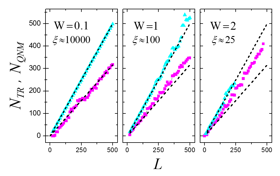
Figure 1: The number of the transmission maxima $N_{T\!R}$ (magenta squares) and the number of quasi normal modes, $N_{Q\!N\!M}$, calculated by integration over the density of states (cyan triangles) for a disordered 1D wire as a function of the length $L$. The cases of: low disorder $\xi\approx 10000$ (left); medium disorder $\xi\approx 100$ (middle); and strong disorder $\xi\approx 25$ (right) are presented. In the low disorder case the number of transmission peaks fits to $N_{\mathrm{tr}}=\mathchoice{{\hbox{$\displaystyle\sqrt{2/5\,}$}\lower 0.4pt\hbox{\vrule height=7.5pt,depth=-6.00003pt}}}{{\hbox{$\textstyle\sqrt{2/5\,}$}\lower 0.4pt\hbox{\vrule height=7.5pt,depth=-6.00003pt}}}{{\hbox{$\scriptstyle\sqrt{2/5\,}$}\lower 0.4pt\hbox{\vrule height=5.25pt,depth=-4.20003pt}}}{{\hbox{$\scriptscriptstyle\sqrt{2/5\,}$}\lower 0.4pt\hbox{\vrule height=3.75pt,depth=-3.00002pt}}}L$ (lower black dashed lines), while the integrated density of states follows $L$ (upper black dashed lines). At higher disorders more transmission resonances are seen (i.e., $N_{\mathrm{tr}}>\mathchoice{{\hbox{$\displaystyle\sqrt{2/5\,}$}\lower 0.4pt\hbox{\vrule height=7.5pt,depth=-6.00003pt}}}{{\hbox{$\textstyle\sqrt{2/5\,}$}\lower 0.4pt\hbox{\vrule height=7.5pt,depth=-6.00003pt}}}{{\hbox{$\scriptstyle\sqrt{2/5\,}$}\lower 0.4pt\hbox{\vrule height=5.25pt,depth=-4.20003pt}}}{{\hbox{$\scriptscriptstyle\sqrt{2/5\,}$}\lower 0.4pt\hbox{\vrule height=3.75pt,depth=-3.00002pt}}}L$) due to localization.

In Fig. 1 we present the results for the number of QNMs, $N_{Q\!N\!M}$, and for the number of the transmission resonances (maxima in $T_{lr}\left(E\right)$), $N_{T\!R}$, as functions of the wire size $L$ for different strengths of disorder (Here and in the remainder of the paper all lengths are presented in units of the lattice constant $a$ which is set to unity).

As can be seen, the dependence of the number of the transmission resonances, $N_{T\!R}$, on $L$ is quite different from that of the number of QNMs. For weak disorder ($W=0.1$, localization length $\xi\sim 10^{4}\gg L$) , $N_{T\!R}$ is much smaller than $N_{Q\!N\!M}$ and equals to $\mathchoice{{\hbox{$\displaystyle\sqrt{2/5\,}$}\lower 0.4pt\hbox{\vrule height=7.5pt,depth=-6.00003pt}}}{{\hbox{$\textstyle\sqrt{2/5\,}$}\lower 0.4pt\hbox{\vrule height=7.5pt,depth=-6.00003pt}}}{{\hbox{$\scriptstyle\sqrt{2/5\,}$}\lower 0.4pt\hbox{\vrule height=5.25pt,depth=-4.20003pt}}}{{\hbox{$\scriptscriptstyle\sqrt{2/5\,}$}\lower 0.4pt\hbox{\vrule height=3.75pt,depth=-3.00002pt}}}L$. The rest of the QNMs are hidden, exactly as it is in optical systems considered in Ref. Bliokh2015 . As the disorder becomes stronger, the hidden (with no transmission resonances) modes gradually reappear as peaks in the transmission function. This can be seen in the increase of the slope of $N_{T\!R}$ versus $L$ dependence with increasing $W$. For stronger disorder this ratio tends to one.

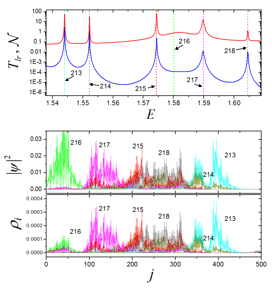
Figure 2: Upper frame: Typical density of states $\mathcal{N}(E)$ (red solid line) and transmission $T_{lr}\left(E\right)$ (blue solid line) spectra of a particular realization of disorder ($L=500$, $W=1$, $t_{l/r}=1$). The positions of the isolated Hamiltonian eigenvalues $\epsilon_{i}$ are indicated by the vertical dashed lines. Middle frame: The squared eigenvectors $|\psi_{i}(r)|^{2}$ of the isolated Hamiltonian as function of the position along the wire, $j$. The 216-th eigenstate is located close to the system edge and therefore its transmission resonance is washed out (see upper frame) when the wire is coupled to the leads. Lower frame: The local density of states integrated in the vicinity of the $i$-th disconnected eigenvalue $\epsilon_{i}$, $\rho_{i}(r)=\int_{\epsilon_{i}-\Delta/4}^{\epsilon_{i}+\Delta/4}\rho\left(r,E\right)dE$. For most states $\rho_{i}(r)\sim|\psi_{i}(r)|^{2}$, except for the hidden mode (the 216-th eigenstate) for which the local density close to the leads is strongly suppressed.

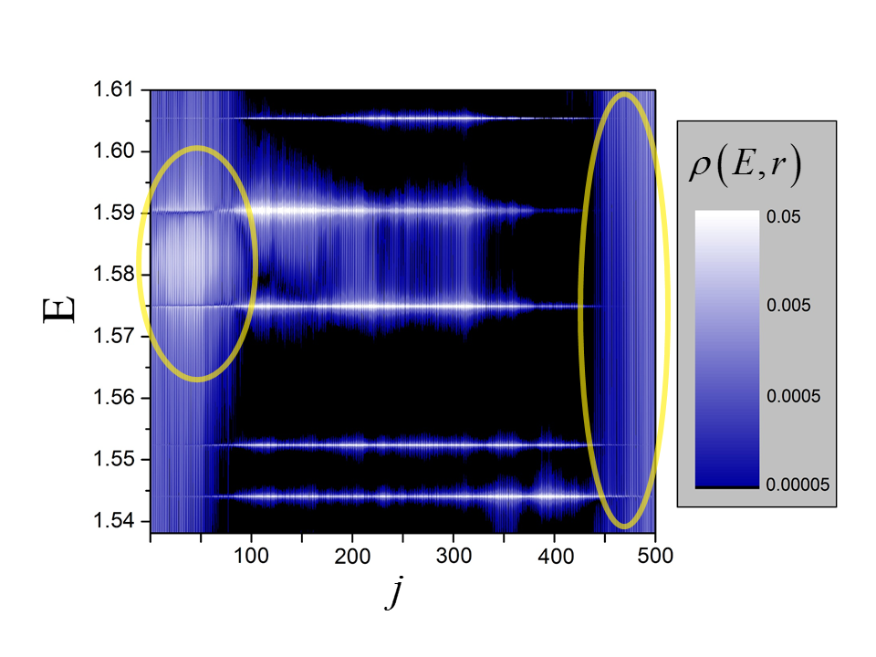
Figure 3: A color map of the local density of states $\rho(j,E)$ of the system described in Fig. 2. The ‘ordinary’ modes (at $E\sim 1.544,1.552,1.575,1.59,1.604$) show relatively narrow energy distribution, while the hidden mode originally located at $E\sim 1.58$ (marked with yellow circle on the left) is significantly broadened due to the coupling to the left lead. Similar hidden mode’s tail can be noticed at the right end, related to a state hidden at higher energy (long yellow circle).

To understand the nature of the ‘hidden’ states let us juxtapose the transmission peaks of the eigen-vectors of the disconnected wire. In the upper panel in Fig. 2 we plot $\mathcal{N}(E)$ and $T_{lr}\left(E\right)$ for a typical realization of disorder in a $L=500$ wire with $W=1$, $\xi\sim 10^{2}$. The corresponding modulus-squared eigen-vectors for the isolated system $|\psi_{i}(r)|^{2}$ are plotted in the middle panel. It is easy to see that each transmission peak (and the associated peak in DOS) corresponds to an eigenstate of the isolated wire, and the peaks in $\mathcal{N}(E)$ and $T_{lr}(E)$ are close to the real eigenvalue $\epsilon_{i}$ (indicated by vertical dashed lines). However the hidden state #216 does not show any peak in the transmission, and the DOS exhibits only a very broad maxima at this eigenvalue. The distinction between hidden and ordinary states shows up also in the local density of states, which for an $i_{th}$ eigenstate we define as $\rho_{i}(r)=\int_{\epsilon_{i}-\Delta/4}^{\epsilon_{i}+\Delta/4}\rho\left(r,E\right)dE$ ,where $\epsilon_{i}$ is the level’s-eigen energy and $\Delta$ is the level spacing. Indeed, while for the ordinary states the local DOS of the connected wire is similar to the density of the disconnected wire i.e., $\rho_{i}(r)\sim|\psi_{i}(r)|^{2}$, for the hidden mode (state $216$) there is a huge difference between $\rho_{216}(r)$ and $|\psi_{216}(r)|^{2}$ (see lower frame of Fig. 2).

In Fig. 3, the LDOS map of the above system in the relevant energy range is presented. The hidden mode originally located at $E=1.58$ (#216) is broadened much beyond the mean level spacing. The spatial distributions of the two types of states are also quite different. Namely, the hidden ones are always nestled against an edge of the sample, so that when the wire is coupled to the leads, these modes become strongly hybridized with the states of the neighboring lead and do not reach the opposite edge of the sample.

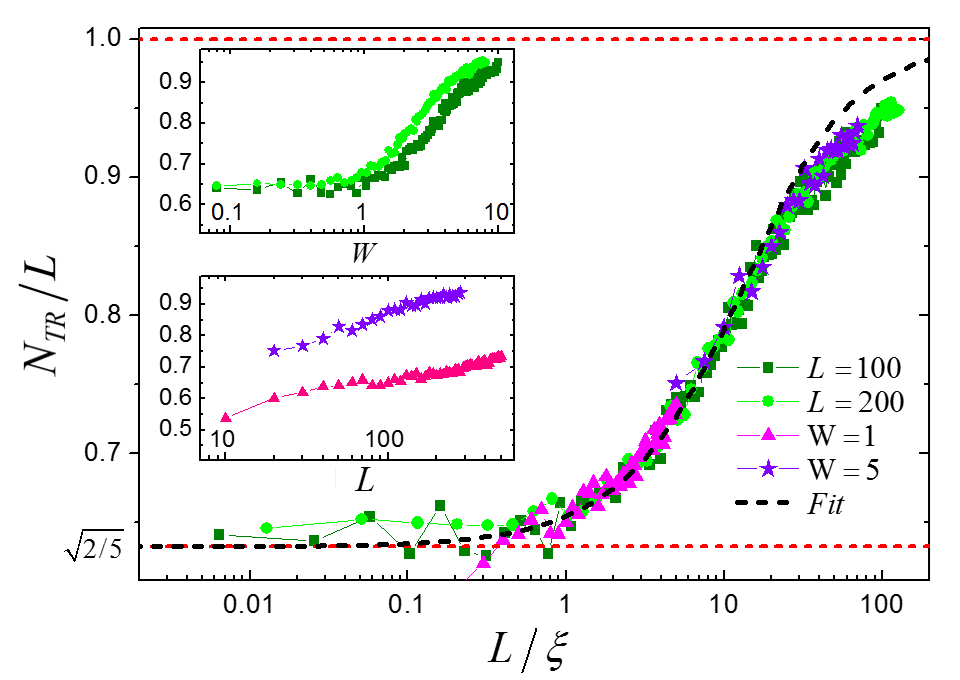
Figure 4: The ratio of the number of observed transmission peaks to the length of the wire $N_{\mathrm{tr}}/L$ for various disorder strength, $W$, and wire length $L$. Upper inset: Systems with length $L=100$ and $L=200$ for various disorder values. Lower inset: Systems with disorder strength $W=1$ and $W=5$ for various lengths. Main panel: the ratio $N_{\mathrm{tr}}/L$ as a function of the scaling parameter $L/\xi$ for the results presented in the insets. All curves of $N_{\mathrm{tr}}/L$ fall on top each other. For $L/\xi<1$, $N_{\mathrm{tr}}/L\sim\mathchoice{{\hbox{$\displaystyle\sqrt{2/5\,}$}\lower 0.4pt\hbox{\vrule height=7.5pt,depth=-6.00003pt}}}{{\hbox{$\textstyle\sqrt{2/5\,}$}\lower 0.4pt\hbox{\vrule height=7.5pt,depth=-6.00003pt}}}{{\hbox{$\scriptstyle\sqrt{2/5\,}$}\lower 0.4pt\hbox{\vrule height=5.25pt,depth=-4.20003pt}}}{{\hbox{$\scriptscriptstyle\sqrt{2/5\,}$}\lower 0.4pt\hbox{\vrule height=3.75pt,depth=-3.00002pt}}}$ remains. Once $L/\xi>1$ , the ratio increases until $N_{\mathrm{tr}}/L\rightarrow 1$ for large values of $L/\xi$, i.e., for strong localization all modes have transmission resonances. The black dashed line represents the dependence of the $N_{\mathrm{tr}}/L$ on $L/\xi$ according to Eq. (22-23) with $b=1/4$.

Numerical calculations show that at weak disorder, when where $\xi$ is larger than the system size, only $\mathchoice{{\hbox{$\displaystyle\sqrt{2/5\,}$}\lower 0.4pt\hbox{\vrule height=7.5pt,depth=-6.00003pt}}}{{\hbox{$\textstyle\sqrt{2/5\,}$}\lower 0.4pt\hbox{\vrule height=7.5pt,depth=-6.00003pt}}}{{\hbox{$\scriptstyle\sqrt{2/5\,}$}\lower 0.4pt\hbox{\vrule height=5.25pt,depth=-4.20003pt}}}{{\hbox{$\scriptscriptstyle\sqrt{2/5\,}$}\lower 0.4pt\hbox{\vrule height=3.75pt,depth=-3.00002pt}}}N$ transmission peaks exist, exactly as it is in the case of weakly scattered electromagnetic waves. However, for stronger disorder where $\xi<L$, only a small fraction (of order $2\xi/L$) of the states hybridize with the leads. States which do not hybridize with the leads might have very small transmission, but nevertheless, they do have a transmission peak. Thus, we expect that $N_{T\!R}/L$ will scale with $\xi/L$. Indeed as can be seen in Fig. 4 , this seems to hold for different values of $L$ and disorder strength $W$.

One can cast the above argument in a more quantitative form. The overlap of a localized state with the left lead should be proportional to $\exp(-bj_{0}/\xi)$, where $j_{0}$ is the center of the localized state and $b$ is a numerical constant of order of one depending on the details of the boundary condition. Averaging over the region $0<j_{0}<L/2$ for the left lead and $L/2<j_{0}<L$ for the right lead, results in:

$$f=\frac{2}{L}\cdot\sum_{j_{0}=1}^{L/2}{e^{-bj_{0}/\xi}}=\left(\frac{2}{L}\right)\frac{1-e^{-bL/2\xi}}{e^{b/\xi}-1}$$ (22)

$$\sim\left(\frac{2\xi}{bL}\right)\left(1-e^{-bL/2\xi}\right)$$

Finally, the ratio of the number of transmission peaks to the length of the wire is obtained by subtracting the fraction of hidden modes times the probability they overlap with the leads, i.e.,

$$N_{T\!R}/L=1-f\cdot\left(1-\mathchoice{{\hbox{$\displaystyle\sqrt{2/5\,}$}\lower 0.4pt\hbox{\vrule height=7.5pt,depth=-6.00003pt}}}{{\hbox{$\textstyle\sqrt{2/5\,}$}\lower 0.4pt\hbox{\vrule height=7.5pt,depth=-6.00003pt}}}{{\hbox{$\scriptstyle\sqrt{2/5\,}$}\lower 0.4pt\hbox{\vrule height=5.25pt,depth=-4.20003pt}}}{{\hbox{$\scriptscriptstyle\sqrt{2/5\,}$}\lower 0.4pt\hbox{\vrule height=3.75pt,depth=-3.00002pt}}}\right),$$ (23)

which after fitting the parameter $b$ reasonably matches the numerical results (Fig. 4).

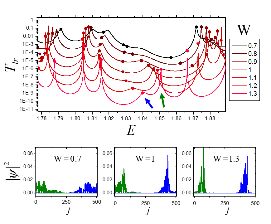
Figure 5: Upper frame: The transmission $T_{lr}\left(E\right)$ for a given realization of disorder at different strengths $W$ from $0.7$ (top black line) to $1.3$ (bottom red line), for a $L=500$ sample with $t_{l/r}=1$. The eigen-energies of the corresponding isolated wires are marked by circles. Two modes are hidden at low $W$, and become visible only at higher disorder level (marked by arrows). Lower frame: The modulus-square of the isolated eigen-vectors related the two above hidden states. As the disorder increased, the width of the modes becomes smaller and eventually they disassociate from the states of the wire.

In Fig. 5 we demonstrate the evolution of the transmission spectrum with increasing strength of disorder. As $W$ grows, the hidden modes gradually disconnect from the boundaries of the wire and form transmission resonances, until all of them become ordinary, $N_{T\!R}/L\rightarrow 1$, for large $W$.

It is also interesting to note that the height of the transmission peak is a non-monotonous function of $W$. While naively one may expect that peaks will reduce as disorder became stronger, this is correct only on average, and particular peaks may actually increase when disorder increases.

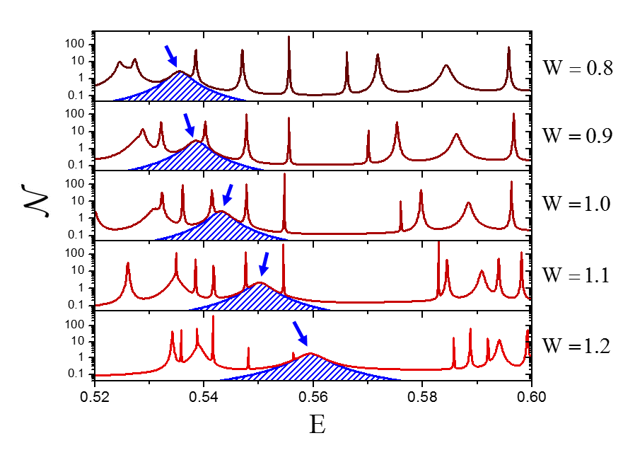
Figure 6: Density of states $\mathcal{N}(E)$ of the system depicted in Fig. 5 at different energies, as disorder increases. The ordinary states become narrower at larger fluctuations, while the hidden mode (marked with blue arrows) widens. Fit to Lorenzian broadening in accordance with Eq. 24 (blue patterned areas) results in $\gamma_{i}^{0.8}\!=\!0.00165$, $\gamma_{i}^{0.9}\!=\!0.00168$, $\gamma_{i}^{1.0}\!=\!0.00172$, $\gamma_{i}^{1.1}\!=\!0.00201$ and $\gamma_{i}^{1.2}\!=\!0.00249$, i.e. shorter lifetime at the higher disorder level (see text).

The spectral broadening of the wire eigenstates (or of the imaginary parts of the eigenvalues in the Hamiltonian language) is inversely related to their lifetime. In disordered open systems, as the localization length becomes shorter (i.e., larger potential fluctuation), one can expect all modes’ lifetimes to increase. This indeed is the case for regular modes, as seen in Fig. 6. However, the hidden states again behave in an unusual way, and remain wide. One can showDatta1995 that if the self energy term (Eq. (14)) varies slowly with $E$, the DOS broadening has a Lorentzian shape:

$$\mathcal{N}(E)\propto\displaystyle\sum_{i}\frac{\gamma_{i}}{(E-\tilde{E}_{i})^{2}+(\gamma_{i})^{2}}$$ (24)

where $\gamma_{i}$ is the imaginary part of the $i_{th}$ eigenvalue, and $\tilde{E}_{i}$ is its real part, modified by the connection to the leads. This relation allows one to evaluate the lifetime of the $i_{th}$ mode, $\hbar/4\gamma_{i}$, by fitting $\mathcal{N}(E)$ to Eq. (24). For the system depicted in Fig. 6, the life time of the hidden mode at lower disorder ($W=0.8$, $\gamma_{i}=0.00165$) is longer than at the higher disorder ($W=1.2$, $\gamma_{i}=0.00249$).

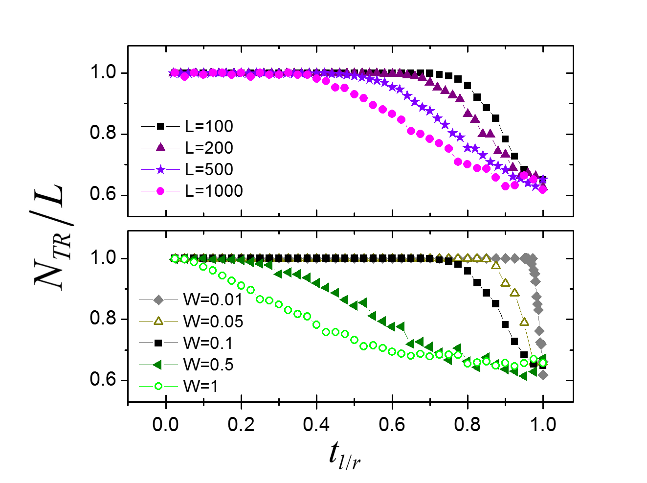
Figure 7: The ratio of the number of observed transmission peaks to the length of the wire $N_{T\!R}/L$ versus lead-system coupling strength, $t_{l/r}$. Top panel: $W=0.1$ for different system length $L$. Bottom panel: $L=100$ for different disorder strength $W$. For both cases as $t_{l/r}\rightarrow 0$, $N_{T\!R}/L\sim 1$, while for $t_{l/r}\rightarrow 1$ $N_{T\!R}/L\sim\mathchoice{{\hbox{$\displaystyle\sqrt{2/5\,}$}\lower 0.4pt\hbox{\vrule height=7.5pt,depth=-6.00003pt}}}{{\hbox{$\textstyle\sqrt{2/5\,}$}\lower 0.4pt\hbox{\vrule height=7.5pt,depth=-6.00003pt}}}{{\hbox{$\scriptstyle\sqrt{2/5\,}$}\lower 0.4pt\hbox{\vrule height=5.25pt,depth=-4.20003pt}}}{{\hbox{$\scriptscriptstyle\sqrt{2/5\,}$}\lower 0.4pt\hbox{\vrule height=3.75pt,depth=-3.00002pt}}}$.

Since the number of observed transmission resonances depends on both the disorder and coupling to the environment, the ratio $N_{\mathrm{tr}}/L$ can be tuned by varying $t_{l/r}$. As this coupling parameter decreases, hidden modes decouple from the leads and develop peaks in the transmission spectrum. As can be seen in Fig. 7, at weak disorder ($W=0.01$) this transition is sharp: all hidden modes become visible for a very small change at the vicinity of $t_{l/r}\sim 1$. As the disorder increases (or the system becomes longer) the coupling amplitude needed to resolve all transmission resonances becomes smaller and the jump in the ratio $T_{\mathrm{tr}}/L$ broadens. This behavior is counter-intuitive, as one may think that the enhancement of fluctuations of the potential makes the sample more “closed”, and therefore will be more easily disconnected from the leads. In fact, the disorder ties the electronic states strongly to their position in the sample (the edges in the case of hidden modes) and therefore a lower $t_{l/r}$ is required in order to disconnect them.

The appearance of two time scales when the coupling to the environment increases and QNMs begin to overlap has been observed in a variety of regular open physical systems Celardo2009 ; Celardo2010 ; Persson2000 ; Sanchez2011 ; Morales2012 ; Aberg2008 ; for a review, see Auerbach2011 and references therein. This phenomenon is rather general and is known as the superradiance transition. Its essence is the following: At weak coupling to the environment the lifetimes of all states goes down as the coupling increases. As the coupling reaches a critical value, the states separate into short-lived (superradiant) and long-lived (trapped) ones, much like the partition of QNMs into ordinary and hidden modes shown in Fig. 7. However, along with the similarity between the resonance trapping in regular open optical and microwave structures, and between “hiding” of some of the resonances in disordered wires there are substantial differences as well. Indeed, crucial for the superradiance transition are the edge barriers that provide tunable (from very weak and up) coupling of the system with the environment. Superradiant modes appear in regular systems regardless of disorder, which just introduces new features (for example, the critical value of the coupling increases with the degree of disorder Auerbach2011 ) but does not change the essence of the phenomenon. In the random samples that we consider, finite coupling is implemented by disorder, as the result of the interference of multiply-scattered random fields, even when the system is completely open. Hidden states appear at the very onset of disorder, when the localization length is much larger than the size of the samples. When the disorder increases, the states remain hidden for a wide range of the disorder strength, and gradually transform into ordinary QNMs as the system reaches the localized regime.

While the transmission is the natural quantity to measure for optical systems, in electronic systems it is much more commonplace to measure conductivity. Measuring conductivity is different than measuring transmission in several aspects. Unlike the ease of generating a single-mode laser beam, electrons are naturally widely distributed in the energy domain due to thermal broadening. Therefore, observing the conductance peaks is possible only if the mean level spacing, $\Delta$, is larger than $k_{B}\!\mathcal{T}$. Thus the ratio of the number of observable conductance peaks, $N_{cp}$, to the system length $N_{cp}/L$ falls to zero as $k_{B}\!\mathcal{T}/\Delta\sim 1$. This crossover for different wire length and temperatures is plotted in Fig.8. The smearing of the conductance peaks for $k_{B}\!\mathcal{T}>\Delta$ is clearly seen.

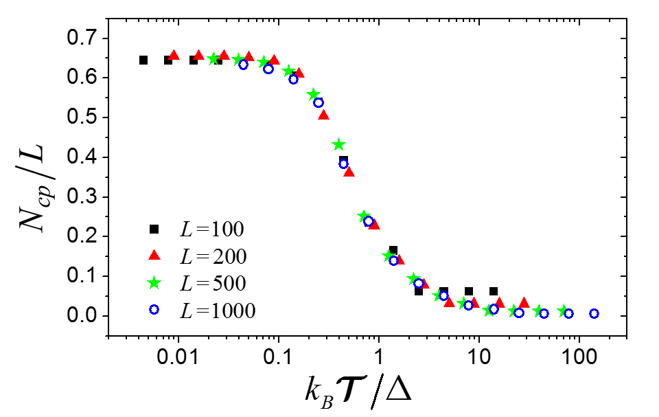
Figure 8: The ratio between the number of conductance peaks $N_{cp}$ and the length $L$ for different values of temperatures $k_{B}\!\mathcal{T}$ and $L$, for a low bias $V=0.001$ and small disorder $W=0.1$. The temperature smears some of the conduction peaks and reduces $N_{cp}$ as it grows. The ratio is scaled by $k_{B}\!\mathcal{T}/\Delta$ where $\Delta\sim 4t/L$ is the single level spacing of the disconnected wire. The transition from zero temperature behavior $N_{cp}/L\sim\mathchoice{{\hbox{$\displaystyle\sqrt{2/5\,}$}\lower 0.4pt\hbox{\vrule height=7.5pt,depth=-6.00003pt}}}{{\hbox{$\textstyle\sqrt{2/5\,}$}\lower 0.4pt\hbox{\vrule height=7.5pt,depth=-6.00003pt}}}{{\hbox{$\scriptstyle\sqrt{2/5\,}$}\lower 0.4pt\hbox{\vrule height=5.25pt,depth=-4.20003pt}}}{{\hbox{$\scriptscriptstyle\sqrt{2/5\,}$}\lower 0.4pt\hbox{\vrule height=3.75pt,depth=-3.00002pt}}}$ to the high temperature behavior $N_{cp}/L\sim 0$ occurs around $k_{B}\!\mathcal{T}/\Delta=1$

V.1 Conclusions

In this paper, we discussed the effect of disorder on the transmission and conductivity resonances. We have shown that, similarly to disordered optical systems, in a 1-D wire with on-site random potential there exists a ballistic regime, in which a significant amount of eigen-states do not show a clear peaks in transmission measurements. These ‘hidden’ modes have extremely broad spectral distributions which, contrary to ordinary Anderson modes, become even broader (i.e. have shorter life-time) as the disorder increases. The primary cause of this phenomena is the hybridization with the states of the attached open leads, which falls off as the localization length $\xi$ becomes shorter than the system length $L$, or as the coupling to the leads is reduced. For weak disorder, the averaged ratio of the number of the hidden modes to the total number of the electron states in a given energy interval deviates only slightly from the constant, $1-\mathchoice{{\hbox{$\displaystyle\sqrt{\nicefrac{{2}}{{5}}\,}$}\lower 0.4pt\hbox{\vrule height=6.44444pt,depth=-5.15558pt}}}{{\hbox{$\textstyle\sqrt{\nicefrac{{2}}{{5}}\,}$}\lower 0.4pt\hbox{\vrule height=4.51111pt,depth=-3.6089pt}}}{{\hbox{$\scriptstyle\sqrt{\nicefrac{{2}}{{5}}\,}$}\lower 0.4pt\hbox{\vrule height=3.22221pt,depth=-2.57779pt}}}{{\hbox{$\scriptscriptstyle\sqrt{\nicefrac{{2}}{{5}}\,}$}\lower 0.4pt\hbox{\vrule height=3.22221pt,depth=-2.57779pt}}}$, as the fluctuations of the potential and/or the length of the wire increase. This constant coincides with the value analytically calculated in the single-scattering approximation. The existence of the hidden modes might substantially affect transport measurements in quantum dots, nanotubes, and topological insulators, at weak and moderate disorder.

VI Appendix: Analytical calculation of the ratio $N_{T\!R}/N_{Q\!N\!M}$

Assuming only single scattering process and free electron wave propagation between scatterers, the transmission probability of an electron with momentum $k$ in a wire with on-site disorder can be written as:

$$T\left(k\right)=1-\left|r\left(k\right)\right|^{2}=1-\left|\sum_{n=1}^{L}r_{n}\cdot e^{i2kan}\right|^{2},$$ (25)

where $r_{n}$ is the random reflection amplitude at site $n,$ and $a$ is the lattice constant. For convenience, we introduce the unit-less length scale so that $a=1$. Transmission resonances are defined as local maxima of the transmission coefficient $T\left(k\right)$ so that the resonant values of the momentum, $k_{n},$ are the roots of the equation $\frac{dT(k_{n})}{dk}=\frac{d\left|r\left(k\right)\right|^{2}}{dk}=0$, which can be presented as

$$\sum_{n=1}^{N}\sin(2kn)\cdot A_{n}=0.$$ (26)

where

$$A_{n}=\Sigma_{l=1}^{N-n}r_{n+l}r_{l}n+\Sigma_{l=n}^{N}r_{l-n}r_{l}n.$$

Generally speaking, Eq. 26 is a trigonometric polynomial with random coefficients. The statistics of zeroes of such polynomials have been studied in Edelman1995 . Using the results of Edelman1995 it can be shown that in a certain interval $\Delta k,$ the ensemble-averaged number of the real roots $N_{\mathrm{root}}$ of the sum in Eq. (26) equals to

$$N_{root}=\frac{2\Delta k}{\pi}\mathchoice{{\hbox{$\displaystyle\sqrt{\frac{\sum_{l=1}^{N}l^{4}(N-l)}{\sum_{l=1}^{N}l^{2}(N-l)}.\,}$}\lower 0.4pt\hbox{\vrule height=28.1235pt,depth=-22.4989pt}}}{{\hbox{$\textstyle\sqrt{\frac{\sum_{l=1}^{N}l^{4}(N-l)}{\sum_{l=1}^{N}l^{2}(N-l)}.\,}$}\lower 0.4pt\hbox{\vrule height=19.7251pt,depth=-15.78015pt}}}{{\hbox{$\scriptstyle\sqrt{\frac{\sum_{l=1}^{N}l^{4}(N-l)}{\sum_{l=1}^{N}l^{2}(N-l)}.\,}$}\lower 0.4pt\hbox{\vrule height=14.64172pt,depth=-11.71342pt}}}{{\hbox{$\scriptscriptstyle\sqrt{\frac{\sum_{l=1}^{N}l^{4}(N-l)}{\sum_{l=1}^{N}l^{2}(N-l)}.\,}$}\lower 0.4pt\hbox{\vrule height=14.64172pt,depth=-11.71342pt}}}$$ (27)

Calculating the sums in Eq. (27) in the limit $N\gg 1$, one gets Gradshteyn2007

$$N_{root}\approx\frac{2a\Delta kN}{\pi}\mathchoice{{\hbox{$\displaystyle\sqrt{\frac{2}{5}\,}$}\lower 0.4pt\hbox{\vrule height=9.66666pt,depth=-7.73337pt}}}{{\hbox{$\textstyle\sqrt{\frac{2}{5}\,}$}\lower 0.4pt\hbox{\vrule height=6.76666pt,depth=-5.41336pt}}}{{\hbox{$\scriptstyle\sqrt{\frac{2}{5}\,}$}\lower 0.4pt\hbox{\vrule height=4.83331pt,depth=-3.86667pt}}}{{\hbox{$\scriptscriptstyle\sqrt{\frac{2}{5}\,}$}\lower 0.4pt\hbox{\vrule height=4.83331pt,depth=-3.86667pt}}}.$$ (28)

Since the total number of QNMs in the interval $\Delta k$ is equal to $\Delta kLa/\pi,$ and $N_{T\!R}=N_{root}/2,$ from Eq. (28) it follows that

$$\frac{N_{T\!R}}{N_{Q\!N\!M}}=\mathchoice{{\hbox{$\displaystyle\sqrt{\frac{2}{5}\,}$}\lower 0.4pt\hbox{\vrule height=9.66666pt,depth=-7.73337pt}}}{{\hbox{$\textstyle\sqrt{\frac{2}{5}\,}$}\lower 0.4pt\hbox{\vrule height=6.76666pt,depth=-5.41336pt}}}{{\hbox{$\scriptstyle\sqrt{\frac{2}{5}\,}$}\lower 0.4pt\hbox{\vrule height=4.83331pt,depth=-3.86667pt}}}{{\hbox{$\scriptscriptstyle\sqrt{\frac{2}{5}\,}$}\lower 0.4pt\hbox{\vrule height=4.83331pt,depth=-3.86667pt}}}.$$ (29)

In Fig. 1 it is clearly seen that at the limit of weak disorder ($\xi\gg L$) this relation is perfectly followed by the numerical quantum calculations.

References

References

- (1) Y. P. Bliokh, V. Freilkher, Z. Shi, A. Genack and F. Nori, New J. Phys. 17, 113009 (2015).
- (2) E.S.C. Ching, P.T. Leung, A. Maassen van den Brink, W.M. Suen, S.S. Tong, and K. Young, Rev. Mod. Phys. 70, 1545 (1998).
- (3) R. Pnini and B. Shapiro, Phys. Rev. E 54, R1032 (1996).
- (4) P. T. Leung, S. Y. Liu, and K. Young, Phys. Rev. A 49, 3057 (1994).
- (5) J. Wang, Z. Shi, M. Davy, and A. Z. Genack, Int. J. Mod. Phys. Conf. Ser. 11, 1 (2012).
- (6) J. Wang and A.Z. Genack, Nature 471, 345 (2011).
- (7) N. Moiseev, Non-Hermitian Quantum Mechanics, Cambridge Univ. Press (2011).
- (8) Y. Imry and R. Landauer, Rev. Mod. Phys. 71 S306 (1999).
- (9) C.W.J. Beenakker, Rev. Mod. Phys. 69, 731 (1997).
- (10) P. W. Anderson, Phys. Rev. 124, 41 (1961).
- (11) S. Datta, ”Electric Transport in Mesoscopic Systems”, Cambridge Press (1995).
- (12) R.A. Römer and M. Schreiber, Phys. Rev. Lett. 78, 515 (1997).
- (13) G. Celardo, L. Kaplan, Phys. Rev. B 79, 155108 (2009).
- (14) G. Celardo, A. Smith, S. Sorathia, V. Zelevinsky, R. Sen’kov, L. Kaplan, Phys. Rev. B 82, 165437 (2010).
- (15) E. Persson, I. Rotter, H-J. Stöckmann, M. Barth, Phys. Rev. Lett. 85, 2478 (2000).
- (16) C. Sanchez-Perez, K. Volke-Sepulveda, J. Flores, Progress In Electromagnetics Research Symp. Proc. p.209 (2011).
- (17) A. Morales, A. Diaz-de-Anda, J. Flores, L. Gutierrez, L. Mendez-Sanchez, G. Monsivais, P. Mora Europhys. Lett. 99, 54002 (2012).
- (18) S. Aberg, T. Guhr , M. Miski-Oglu, A. Richter, Phys. Rev. Let. 100, 204101 (2008).
- (19) N. Auerbach, V. Zelevinsky, Rep. Prog. Phys. 74, 106301 (2011).
- (20) A. Edelman and E. Kostlan, Bull. Amer. Math. Soc. 32, 14 (1995).
- (21) I.S. Gradshteyn and I. M. Ryzhik ”Table of Integrals, Series, and Products”, 7th edn, New York: Academic, pp. 1–2 (2007).