Rotational diffusion under torque: Microscopic reversibility and excess entropy

Abstract

We consider rotational diffusion for two systems - a macrospin under external magnetic field, and a particle diffusing on the surface of a sphere under external torque. Microstates in the two cases transform differently under time-reversal. This results in Clausius like dependence of stochastic entropy production (EP) for macrospins, and an excess EP for diffusion of particles on sphere. The total EP in both the cases obey fluctuation theorems. For macrospins, we derive analytical expression for probability distribution of total EP in the adiabatic limit. Numerical simulations show that the distribution functions of EP agree well with theoretical predictions.

I Introduction

Stochastic thermodynamics has extended the definitions of thermodynamic quantities like work, energy, entropy etc. to their stochastic counterpart, as a description of stochastic evolution of non-equilibrium systems with small degrees of freedom Jarzynski2011 ; Seifert2012 . This allows one to obtain energy balance, and equalities involving entropy production (EP), or work done known as fluctuation theorems (FT) Evans1993 ; Gallavotti1995 ; Jarzynski1997 ; Sekimoto1998 ; Lebowitz1999 ; Crooks1999 ; Seifert2005 ; Baiesi2009 ; Baiesi2010 ; Hummer2010 ; Kurchan2007 ; Narayan2004 ; Jayannavar2007 ; Lahiri2014a ; Saha2009 ; Lahiri2009 ; Sahoo2011 . In experiments FT symmetries were observed Wang2002 ; Blickle2006 ; Speck2007 ; Joubaud2012 , and used to extract free energies from non-equilibrium measurements Liphardt2002 ; Collin2005 . The ideas of stochastic thermodynamics have been extended to active particles as well Hayashi2010 ; Seifert2011 ; Ganguly2013 ; Chaudhuri2014 .

Stochastic energy balance can be derived from appropriate Langevin equations giving the definition of dissipated heat. This does not depend on how the microscopic dynamical variables transform under time-reversal operation. However, EP captures breaking of time-reversal symmetry, and does depend on how microstates transform under time-reversal operation. In this paper, using two systems whose dynamics are given by the same equation of motion, but whose microstates transform differently under time-reversal, we demonstrate how the EP in them are different. While one of these systems show stochastic reservoir EP consistent with Clausius expression, the other gives rise to an excess EP which can not be captured by the dissipated heat. We focus on stochastic thermodynamics of macrospins having a single magnetic domain, and a related system of particles diffusing on the surface of a unit sphere.

With advent of spintronics, magnetic devices are getting miniaturized. In such devices, macrospins reside in a complex magnetic environment that may produce time varying torque. The impact of thermal fluctuations increases inversely with reducing size of devices Blanter2000 ; Jr1963 ; Coffey2012 , giving rise to drastic effects like magnetization reversal Parkin2000 . Several recent studies focussed on how to control magnetic devices against thermal noise Tserkovnyak2001 ; Foros2005 ; Foros2007 ; Bandopadhyay2011 ; Covington ; Utsumi2015 . In Ising spins following Glauber dynamics, distribution of dissipative work was presented in Ref. Marathe2005 . Unlike Ising spins, macrospins in presence of magnetic fields undergo stochastic rotational motion. The diffusion of a particle on unit sphere in presence of external torque, is described by Langevin equations closely related to that describing the stochastic macrospin dynamics. However, the origin of torque does not anymore come from a conservative magnetic energy density, rather is imposed externally. Also, the notion of dissipative and reactive currents depend on the transformation of angular positions identifying microstates. While magnetic field and magnetization are odd variables under time reversal, angular position of diffusing particle and external torque are even variables, leading to different forms of EP.

II Macrospin

First let us consider a macrospin with magnetization ${\bf m}$ in presence of a time-dependent magnetic field ${\bf H}(t)$. The deterministic dynamics $\dot{\bf m}=\gamma{\bf m}\times{\bf H}(t)$, where $\dot{\bf m}=d{\bf m}/dt$, and $\gamma$ denotes the gyromagnetic ratio, conserves magnetization $dm^{2}/dt={\bf m}.\dot{\bf m}=0$. For a time-independent field ${\bf H}$, the macrospin precesses around the field due to spin torque ${\bf m}\times{\bf H}$. Stochastic dynamics of macrospin may involve fluctuations in both amplitude and direction of magnetization Ma2012 ; Bandopadhyay2015 . However, for materials with high enough Curie temperatures, one may neglect the amplitude fluctuation Jr1963 ; Jayannavar1991 ; Seshadri1982 ; Bandopadhyay2015a . This naturally leads to a Langevin dynamics known as the Landau-Lifshitz-Gilbert equation which involves a multiplicative noise. The macrospin coupled to a heat bath gets influence from the heat bath in terms of a stochastic field ${\bf h}(t)$ and a related dissipation with a damping coefficient $\eta$ such that Kubo1962 ; Jr1963 ; Kubo1970

$$\dot{\bf m}=\gamma\,{\bf m}\,\times\,\left[{\bf H}+{\bf h}(t)-\eta\dot{\bf m}\right].$$ (1)

The stochastic magnetic field obeys Gaussian statistics with

$$\langle{\bf h}(t)\rangle = 0,$$

$$\langle{\bf h}(t)\otimes{\bf h}(t^{\prime})\rangle = 2D_{0}{\bf 1}\delta(t-t^{\prime})$$ (2)

where ${\bf 1}$ denotes the identity matrix, $D_{0}=\eta k_{B}T/V$ with $T$ denoting the temperature, $k_{B}$ the Boltzmann constant, and $V$ the volume of the magnetic particle. The LLG equation may be derived using the Zwanzig formalism, coupling the macrospin with a heat bath composed of either spins Seshadri1982 or harmonic oscillators Jayannavar1991 . The magnetic field ${\bf H}$ is obtainable from an energy density $G=-{\bf m}.{\bf H}$ by using ${\bf H}=-\partial G/\partial{\bf m}$.

The rotational diffusion of the orientation ${\bf m}$ on the surface of a sphere of radius $m$ may be represented in terms of angular position $[\theta(t),\phi(t)]$. The Langevin dynamics can then be expressed as

$$\dot{\theta} = h^{\prime}\,m(H_{\theta}+h_{\theta})-g^{\prime}m(\sin\theta)^{-1}(H^{\prime}_{\phi}+h_{\phi})$$

$$\sin\theta\,\dot{\phi} = g^{\prime}m(H_{\theta}+h_{\theta})+h^{\prime}m(\sin\theta)^{-1}(H^{\prime}_{\phi}+h_{\phi}),$$

where

$$g^{\prime}=\frac{1/\gamma m}{(1/\gamma^{2})+\eta^{2}m^{2}},\,h^{\prime}=\frac{\eta}{(1/\gamma^{2})+\eta^{2}m^{2}}.$$

In Eq.(LABEL:llg2), $\dot{\theta}=\partial_{t}\theta$, $\dot{\phi}=\partial_{t}\phi$, and ${\bf H}=\hat{\theta}H_{\theta}+\hat{\phi}H_{\phi}$ with $H_{\theta}=-({1}/{m})\partial_{\theta}G$, $H^{\prime}_{\phi}\equiv H_{\phi}\sin\theta=-({1}/{m})\partial_{\phi}G$. The angular components of stochastic field can be expressed in terms of their cartesian components as $h_{\theta}=h_{x}\cos\theta\cos\phi+h_{y}\cos\theta\sin\phi-h_{z}\sin\theta$, and $h_{\phi}=-h_{x}\sin\theta\sin\phi+h_{y}\sin\theta\cos\phi$. Note that Eq.(LABEL:llg2) involves multiplicative noise. Recently Ref. Aron2014 showed explicitly that the form of FP equation derived from the LLG equation is independent of the choice of stochastic calculus – Ito, Stratonovich or a post-point discretization scheme Lau2007a ; vanKampen1992 . In the following, we use this FP equation which was originally derived in Jr1963 using the Stratonovich convention that we use throughout this paper.

The FP equation corresponding to Eq.(LABEL:llg2) has the form

$$\partial_{t}P=-{\bf\nabla}_{\Omega}.{\bf J}_{\Omega},~{}~{}{\bf J}_{\Omega}=\hat{\theta}J_{\theta}+\hat{\phi}J_{\phi}$$ (4)

where the divergence of current on the right hand side is given by ${\bf\nabla}_{\Omega}.{\bf J}_{\Omega}=\frac{1}{\sin\theta}\partial_{\theta}(\sin\theta J_{\theta})+\frac{1}{\sin\theta}\partial_{\phi}J_{\phi}$, with $\Omega$ denoting the solid angle. The two components of probability current are given by Jr1963

$$J_{\theta} = m[h^{\prime}H_{\theta}-g^{\prime}H_{\phi}]P-k^{\prime}\partial_{\theta}P$$

$$J_{\phi} = m[g^{\prime}H_{\theta}+h^{\prime}H_{\phi}]P-k^{\prime}(\sin\theta)^{-1}\partial_{\phi}P.$$ (5)

Here $h^{\prime}$ and $g^{\prime}$ play the role of mobility, and $k^{\prime}$ plays the role of diffusivity. These mobility and diffusivity coefficients obey Einstein relation $k^{\prime}=D_{0}m^{2}(h^{\prime 2}+g^{\prime 2})=(k_{B}T/V)\,[\eta/(1/\gamma^{2}+\eta^{2}m^{2})]=k_{B}Th^{\prime}/V$ Jr1963 .

Note that equations (LABEL:llg2) and (4) also describe the motion of a particle diffusing on the surface of a sphere under position dependent external torque, with reinterpretation of some of the terms – $m$ should be interpreted as the radius of the sphere, $h^{\prime}$ and $g^{\prime}$ will mean mobility. In absence of $(H_{\theta},H_{\phi})$ the equations describe simple diffusion on a sphere of radius $m$. $[H_{\theta},H_{\phi}]$ acts as an external torque which in general could be any function of $(\theta,\phi,t)$, and need not be derivable from an energy density like $G$. For macrospins, $V$ denotes the total volume of the spin, which can be set to unity for particle diffusion, without any loss of generality. We discuss this dynamics in Sec. III. Note that when treating Eq.s (LABEL:llg2) and (4) as a description of magnetization dynamics, ${\bf m}$ and ${\bf H}$ has to be treated as odd parity variables under time reversal. This reflects in the way ($\theta,\phi$) and $(H_{\theta},H_{\phi})$ transform under time reversal. On the other hand, for a particle diffusing on the surface of a sphere, position ($\theta,\phi$) are even parity variables under time reversal, and in that case $(H_{\theta},H_{\phi})$ having the meaning of externally imposed torque does not change sign under time-reversal. This difference gives rise to two different expressions for EP in the two cases. While for macrospin dynamics one obtains Clausius like relation for EP in the reservoir, for rotation diffusion of particles one finds an excess EP apart from the Clausius term. We show this in detail in the following.

The non-equilibrium Gibbs entropy is given by Crooks1999 ; Seifert2005

$$S=-k_{B}\int d\Omega\,P(\theta,\phi,t)\ln P(\theta,\phi,t)=\langle-k_{B}\ln P\rangle,$$

where $\int d\Omega=\int\sin\theta\,d\theta\,d\phi\,$ is the integration over all possible solid angles, and $\langle\dots\rangle$ denotes statistical average. The above definition of $S$ is the same as the Shanon information entropy of a given probability distribution Shanon1948 ; Kardar2007 . The Szilard engine and Maxwell’s daemon paradox Szilard1929 helped building the connection between Shanon’s information entropy and thermodynamic entropy Maruyama2009 ; Mandal2012 ; Leff1990 . Note that Landauer’s principle linked erasure of one bit of information with minimal heat dissipation by an amount $k_{B}T\ln 2$ Landauer1961 , and this has been experimentally verified Berut2012 . The definition of entropy $S$ thus has a much wider scope, including a description of non-equilibrium processes. The stochastic entropy of a micro-state is given by $s(\theta,\phi,t)=-k_{B}\ln P(\theta,\phi,t)$, such that $S=\langle s\rangle$. One can express the rate of change in stochastic entropy as

$$\frac{\dot{s}}{k_{B}} = -\frac{\partial_{t}P}{P}-\frac{\partial_{\theta}P}{P}\dot{\theta}-\frac{\partial_{\phi}P}{P}\dot{\phi}.$$ (6)

We now consider the two cases of macrospin dynamics under external magnetic field, and diffusion of particle on a sphere in presence of torque, separately.

II.1 Stochastic energy balance

The rate of stochastic energy gain per unit volume $\dot{G}=-{\bf H}\cdot\dot{\bf m}-{\bf m}\cdot\dot{\bf H}$, the rate of work done $\dot{W}=-{\bf m}\cdot\dot{\bf H}$, stochastic heat absorption by the system $\dot{q}=-{\bf H}\cdot\dot{\bf m}$. Thus the stochastic energy balance $\dot{G}=\dot{q}+\dot{W}$. In the spherical polar coordinate,

$$\dot{q}=-{\bf H}\cdot\dot{\bf m} = -[\hat{\theta}H_{\theta}+\hat{\phi}H_{\phi}]\cdot[\hat{\theta}\,m\dot{\theta}+\hat{\phi}\,m\sin\theta\dot{\phi}]$$ (7)

$$= -m\left[H_{\theta}\dot{\theta}+H_{\phi}\sin\theta\,\dot{\phi}\right]\,.$$

Note that the rate of total heat absorption is given by $\dot{Q}=V\dot{q}$.

II.2 Entropy production using Fokker-Planck equation

At this stage, it is crucial to identify the properties of microstate ${\bf m}$ and the probability current ${\bf J}_{\Omega}$ under time reversal. As noted before, ${\bf m}(t)$ and ${\bf H}(t)$ are odd variables under time reversal. The ${\bf m}\to-{\bf m}$ operation is equivalent to taking the spatial configuration $(\theta,\phi)\to(\pi-\theta,\pi+\phi)$. These transformations lead to: $\sin\theta\to\sin\theta$, $\partial_{\theta}\to-\partial_{\theta}$ and $\partial_{\phi}\to\partial_{\phi}$; and as a result $H_{\theta}\to-H_{\theta}$ and $H_{\phi}\to H_{\phi}$.

The original FP equation can be expressed as $\partial_{t}P=-{\bf\nabla}_{\Omega}.({\bf J}_{\Omega}^{(r)}+{\bf J}_{\Omega}^{(d)})$, where ${\bf J}_{\Omega}^{(r)}$ denotes reactive current and ${\bf J}_{\Omega}^{(d)}$ denotes dissipative current. Under time reversal one obtains $\partial_{t}P=-{\bf\nabla}_{\Omega}.{\bf J}_{\Omega}^{(r)}+{\bf\nabla}_{\Omega}.{\bf J}_{\Omega}^{(d)}$, where ${\bf J}_{\Omega}^{(r)}=(-mg^{\prime}H_{\phi}P,mg^{\prime}H_{\theta}P)$ and the dissipative components of current:

$$J_{\theta}^{(d)} = mh^{\prime}H_{\theta}P-k^{\prime}\partial_{\theta}P$$

$$J_{\phi}^{(d)} = mh^{\prime}H_{\phi}P-k^{\prime}(\sin\theta)^{-1}\partial_{\phi}P.$$ (8)

Using Eq.(6) and expressing $\partial_{\theta}P$ and $\partial_{\phi}P$ in terms of the dissipative currents one gets

$$\frac{\dot{s}}{k_{B}}=-\frac{\partial_{t}P}{P}+\frac{J_{\theta}^{(d)}\dot{\theta}+J_{\phi}^{(d)}\sin\theta\,\dot{\phi}}{k^{\prime}P}+\frac{\dot{Q}}{k_{B}T}.$$ (9)

In obtaining the third term on the right hand side of the above relation, we used the identity $h^{\prime}/k^{\prime}=V/k_{B}T$.

At this point, we perform a two step averaging : (i) over trajectories and (ii) over the ensemble of all possible solid angles $\Omega$ with probability $P(\Omega,t)$. The trajectory average of the components of angular velocity leads to $\langle\dot{\theta}|\,\theta,\phi,t\rangle=J_{\theta}/P$ and $\langle\sin\theta\,\dot{\phi}|\,\theta,\phi,t\rangle=J_{\phi}/P$ Seifert2005 . Note that $J_{\theta}=J_{\theta}^{(d)}-mg^{\prime}H_{\phi}P$ and $J_{\phi}=J_{\phi}^{(d)}+mg^{\prime}H_{\theta}P$. In order to perform averaging over the microstate probability $P(\Omega,t)$, we multiply Eq.(9) throughout by $P(\Omega,t)$ and integrate over $\Omega$. The conservation of probability $\int d\Omega P(\Omega,t)=1$ gives $\int d\Omega\partial_{t}P(\Omega,t)=0$. The resultant expression for the average EP in the system

$$\frac{\langle\dot{s}\rangle}{k_{B}} =\int d\Omega\frac{(J_{\theta}^{(d)})^{2}+(J_{\phi}^{(d)})^{2}}{k^{\prime}P}$$

$$+\frac{mg^{\prime}}{k^{\prime}}\int d\Omega\left[J_{\phi}^{(d)}H_{\theta}-J_{\theta}^{(d)}H_{\phi}\right]+\frac{\langle\dot{Q}\rangle}{k_{B}T}.$$ (10)

Note that $\int d\Omega H_{\theta}H_{\phi}P=0$, due to the inversion symmetry of $H_{\theta}$, $H_{\phi}$ through the centre of the coordinate system. Also one can show that $\int d\Omega H_{\phi}\partial_{\theta}P=0$ and $\int d\Omega H_{\theta}\partial_{\phi}P=0$, using integration by parts. Thus the second term in the above equation vanishes, giving us

$$\dot{S}\equiv\langle\dot{s}\rangle = k_{B}\int d\Omega\frac{(J_{\theta}^{(d)})^{2}+(J_{\phi}^{(d)})^{2}}{k^{\prime}P}+\frac{\langle\dot{Q}\rangle}{k_{B}T}$$

$$= \dot{S}_{t}-\dot{S}_{r}.$$

Note that $\dot{S}_{r}=-\langle\dot{Q}\rangle/T$ is the entropy flux to the environment obeying Clausius theorem. The total average EP in system and environment is

$$\dot{S}_{t}=\dot{S}+\dot{S}_{r}=k_{B}\int d\Omega\frac{(J_{\theta}^{(d)})^{2}+(J_{\phi}^{(d)})^{2}}{k^{\prime}P}\geq 0$$ (12)

in accordance with the second law of thermodynamics. Non-zero dissipative currents $J_{\theta}^{(d)}$ and $J_{\phi}^{(d)}$ quantify the irreversible non-equilibrium processes taking place within the system. Calculations of thermodynamic EP using the FP equation have been presented in other contexts in Ref. Tome2006 ; Tome2010 ; Tome2015 . The definition of stochastic entropy of the system $s=-k_{B}\ln P$, along with the FP equation gave us the stochastic reservoir EP

$$\dot{s}_{r}=-\frac{\dot{Q}}{T}=\frac{mV}{T}\left[H_{\theta}\dot{\theta}+H_{\phi}\,\sin\theta\dot{\phi}\right].$$ (13)

II.3 Detailed balance

At equilibrium, due to time-reversibility, all the components of dissipative current has to vanish separately, such that the average total EP is zero. Considering a time-independent magnetic field applied along the $z$-axis, $G=-mH\cos\theta$, $H_{\phi}=0$. Then $J_{\phi}^{(d)}=0$ implies $P$ is independent of $\phi$. The other constraint $J_{\theta}^{(d)}=0$ gives $dP/P=m(h^{\prime}/k^{\prime})H_{\theta}d\theta$. Integrating this equation, and Using the identities $H_{\theta}=-H\sin\theta$, $h^{\prime}/k^{\prime}=V/k_{B}T$, one obtains $P=\frac{1}{Z(H)}\exp[-GV/k_{B}T]$, where $Z(H)$ denotes the partition function at a given field strength $H$.

II.4 Fluctuation theorems

Assume a macrospin evolves from $t=0$ to $\tau_{0}$ along a trajectory $X=[{\bf m}(t),{\bf H}(t)]$ where time dependent field ${\bf H}(t)$ denotes the protocol of forward process. Let us divide the path into $i=1,2,\dots,N$ segments of time-interval $\delta t$ with $N\delta t=\tau_{0}$. The transition probability $p_{i}^{+}(\theta^{\prime},\phi^{\prime},t+\delta t|\theta,\phi,t)$ on $i$-th segment is controlled by the Gaussian random process with probability $P({\bf h}_{i})=(\delta t/4\pi D_{0})^{1/2}\exp(-\delta t\,{\bf h}_{i}^{2}/4D_{0})$ where ${\bf h}_{i}$ denotes the stochastic noise at $i$-th instant. Denoting Eq.(LABEL:llg2) as $\dot{\theta}=\Theta(\theta,\phi,H_{\theta},H_{\phi})$ and $\dot{\phi}=\Phi(\theta,\phi,H_{\theta},H_{\phi})$, the transition probability on $i$-th segment $p_{i}^{+}={\cal J}_{i}\langle\delta(\dot{\theta}_{i}-\Theta_{i})\delta(\dot{\phi}_{i}-\Phi_{i})\rangle={\cal J}_{i}\int d{\bf h}_{i}P({\bf h}_{i})\delta(\dot{\theta}_{i}-\Theta_{i})\delta(\dot{\phi}_{i}-\Phi_{i})$. The Jacobian of transformation ${\cal J}_{i}={\rm det}[\partial(h_{x_{i}},h_{y_{i}},h_{z_{i}})/\partial(m_{i},\theta_{i},\phi_{i})]_{m_{i}={\rm constant}}$. The probability of the complete path is ${\cal P}_{+}=\prod_{i=1}^{N}p_{i}^{+}$.

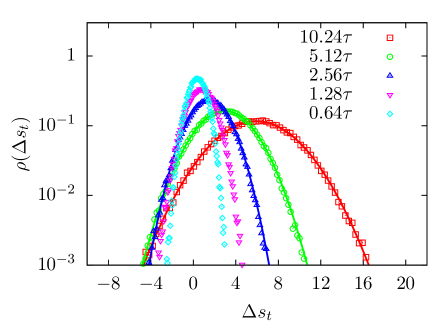
Figure 1: (Color online) Distribution of entropy production for a macrospin initially in absence of magnetic field, driven by a linearly increasing field $H(t)=\alpha\,t$ with time, where the rate $\alpha=H_{f}/\tau_{0}$ with final field strength $H_{f}=0.1\,k_{B}T/m$ at $t=\tau_{0}$. Different curves show entropy distributions calculated over various $\tau_{0}$ denoted in the legend. For $\tau_{0}=2.56,5.12,10.24\,\tau$ the data fit with the analytic form given by Eq.(17) giving $\langle\Delta s_{t}\rangle=5.92,2.96,1.47\,k_{B}$ respectively.

As ${\bf m}$ and ${\bf H}$ are odd variables under time reversal, the time-reversed trajectory can be denoted as $X^{\dagger}=[-{\bf m}(\tau_{0}-t),-{\bf H}(\tau_{0}-t)]$. Replacing $\theta\to\pi-\theta$, and $\phi\to\pi+\phi$ in Eq.(LABEL:llg2) one obtains the equation governing angular dynamics along time reversed trajectories. Denoting these equations as $\dot{\theta}=\Theta^{\dagger}(\theta,\phi,H_{\theta},H_{\phi})$ and $\dot{\phi}=\Phi^{\dagger}(\theta,\phi,H_{\theta},H_{\phi})$, the probability of conjugate trajectory can be expressed as ${\cal P}_{-}=\prod_{i=1}^{N}p_{i}^{-}$, where $p_{i}^{-}={\cal J}_{i}^{-}\langle\delta(\dot{\theta}_{i}-\Theta^{\dagger}_{i}(\tau_{0}-t)\,)\,\delta(\dot{\phi}_{i}-\Phi^{\dagger}_{i}(\tau_{0}-t)\rangle$, where ${\cal J}_{i}^{-}$ denotes the relevant Jacobian. As ${\cal J}_{i}^{-}={\cal J}_{i}$, Jacobians drop out of the ratio $p_{i}^{+}/p_{i}^{-}$ Bandopadhyay2015 . Thus one obtains

$$\frac{\Delta s_{r}}{k_{B}}=\ln\frac{{\cal P}_{+}}{{\cal P}_{-}}=\frac{V\,m}{k_{B}T}\int_{0}^{\tau_{0}}dt\left[H_{\theta}\dot{\theta}+H_{\phi}\sin\theta\dot{\phi}\right].$$ (14)

The above expression of $\Delta s_{r}$ corresponds to $\dot{s}_{r}$ derived from FP equation [see Eq.(13)]. The trajectories considered above describe evolution from a distribution of initial states $P_{i}$ to that of final states $P_{\ell}$, with the change in system entropy

$$\Delta s=k_{B}\ln(P_{i}/P_{\ell}).$$ (15)

Thus the total entropy change $\Delta s_{t}=\Delta s+\Delta s_{r}=k_{B}\ln\frac{{\cal P}^{f}[X]}{{\cal P}^{b}[X^{\dagger}]}$, where total probabilities of time forward and time reversed trajectories are given by ${\cal P}^{f}[X]=P_{i}{\cal P}_{+}$ and ${\cal P}^{b}[X^{\dagger}]=P_{\ell}{\cal P}_{-}$ respectively. As the Jacobian of transformation from $X$ to $X^{\dagger}$ is unity, one readily gets the integral fluctuation theorem (IFT) $\langle e^{-\Delta s_{t}/k_{B}}\rangle=1$, leading to $\langle\Delta s_{t}\rangle\geq 0$ via Jensen inequality.

In a steady state the total entropy change $\Delta s_{t}$ along a time-forward path $\Delta s^{f}_{t}(X)$ is equal and opposite to that along the time-reversed path, $\Delta s^{b}_{t}(X^{\dagger})=-\Delta s^{f}_{t}(X)$. This leads to the detailed fluctuation theorem (DFT) Kurchan2007 ; Crooks1999

$$\rho(\Delta s_{t}) = e^{\Delta s_{t}/k_{B}}\rho(-\Delta s_{t}).$$ (16)

II.5 Distribution of entropy production

Let us consider a time dependent magnetic field ${\bf H}=H(t)\hat{z}$ with linear time-dependence $H(t)=H_{0}+\alpha t$. Writing it in a dimensionless form $mH/k_{B}T=\epsilon(1+\zeta t/\tau)$ where $\epsilon=mH_{0}/k_{B}T$, and $\zeta=\alpha\tau/H_{0}$ is the dimensionless rate of change of the field, with unit of time set by $\tau=m/\gamma k_{B}T$. For slow rate $\zeta\ll 1$ the system remains close to equilibrium, and for fast rate $\zeta\gg 1$ the variation in magnetic field is too fast for the instantaneous magnetization to follow it. From numerical simulations using Stratonovich discretization of Eq.(LABEL:llg2) with time step $\delta t=0.01\tau$ we calculate fluctuations in EP, and obtain its probability distributions at various driving rates. We express the magnetization in units of $m$, and energy in units of $k_{B}T$. In calculating total EP we use the expressions given in Eq.s (14) and (15).

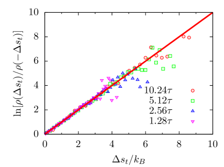
Figure 2: (Color online) Ratio of probability distributions of positive and negative EP, $\ln[\rho(\Delta s_{t})/\rho(-\Delta s_{t})]$ calculated from the data shown in Fig. 1. The solid line is a plot of the function $\Delta s_{t}/k_{B}$. The deviation of data for larger $\Delta s_{t}$ is due to lack of statistics.

Let us change the magnetic field from $0$ to $H_{f}=0.1$ (in units of $k_{B}T/m$) in a time window $\tau_{0}$, which sets the rate $\alpha=H_{f}/\tau_{0}$. The distribution functions for different rates are plotted in Fig.1, and are denoted by the values of $\tau_{0}$. In Fig. 2, the natural logarithm of the ratio of probabilities of positive and negative EP is plotted against EP. This shows good agreement with the prediction of detailed FT. Note that, for slower driving rates ($\tau_{0}\geq 2.56\,\tau$), the distribution functions are broad, and have Gaussian profile (Fig.1). The Gaussian nature can be understood by splitting the total time $\tau_{0}$ into smaller intervals, beyond which fluctuations of magnetization are not correlated. Since the reservoir EP is a sum over many such uncorrelated random events [Eq.(14], one obtains Gaussian distribution in accordance with the central limit theorem,

$$\rho(\Delta s_{t})=\frac{1}{\sqrt{2\pi\sigma^{2}}}e^{-(\Delta s_{t}-\langle\Delta s_{t}\rangle)^{2}/2\sigma^{2}},$$

peaked at the mean EP $\langle\Delta s_{t}\rangle$. Moreover, the distribution should obey the IFT, $\langle e^{-\Delta s_{t}/k_{B}}\rangle=1$. This requires $\sigma^{2}=2k_{B}\langle\Delta s_{t}\rangle$. Thus the distribution of EP is expected to have the form

$$\rho(\Delta s_{t})=\frac{1}{\sqrt{4\pi k_{B}\langle\Delta s_{t}\rangle}}e^{-(\Delta s_{t}-\langle\Delta s_{t}\rangle)^{2}/4k_{B}\langle\Delta s_{t}\rangle}.$$ (17)

The lines in Fig.1 show fit of numerical data to this function.

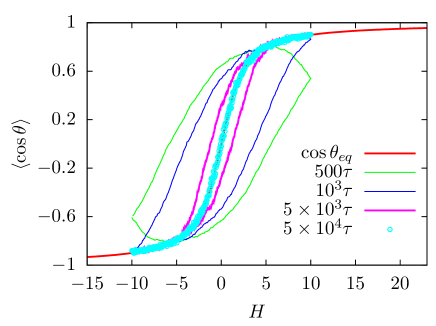
Figure 3: (Color online) Hysteresis curves at non-equilibrium steady states. The curve $\cos\theta_{\rm eq}$ plots the equilibrium Langevin function. The legend denotes time period of changing external field. As the cycle gets extremely slow ($t_{p}=5\times 10^{4}\tau$), $m_{z}/m=\langle\cos\theta\rangle$ collapses onto the equilibrium curve.

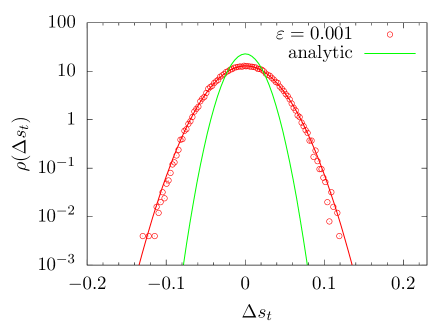
Figure 4: (Color online) Data points denote simulated probability distribution of EP at dimensionless driving rate $\zeta=10^{-3}$ around a field $mH/k_{B}T=2$, integrated over a period of $1.28\tau$. The (red) solid line through data denotes a fit to Eq.(17) giving $\langle\Delta s_{t}\rangle=4.8\times 10^{-4}k_{B}$. The (green) line labeled analytic plots the function in Eq.(17) with $\langle\Delta s_{t}\rangle=1.5\times 10^{-4}k_{B}$ obtained from Eq.(19).

In principle, the mean EP $\langle\Delta s_{t}\rangle$ may be obtained from Eq.(12), using numerical methods. However, in the limit of $\zeta\ll 1$, one may use adiabatic approximation to calculate $\langle\Delta s_{t}\rangle$ over a time $t$. In presence of a uniaxial field, Eq.(7) gives $\dot{q}=-mH_{\theta}\dot{\theta}$. Within mean field approximation $\langle\dot{q}\rangle\approx-m\langle H_{\theta}\rangle\langle\dot{\theta}\rangle=-m^{2}H^{2}h^{\prime}\langle\sin\theta\rangle^{2}$. At equilibrium, the magnetization along external field $m_{z}/m=\langle\cos\theta\rangle$ is given by the Langevin function,

$$\langle\cos\theta\rangle_{\rm eq}\equiv\cos\theta_{\rm eq}=\left[\coth\epsilon-\frac{1}{\epsilon}\right],$$ (18)

where, $\epsilon=mH/k_{B}T$. Within adiabatic approximation, replacing $H$ by $H(1+\zeta\,t/\tau)$, one finds $\cos\theta_{\rm ad}=\cos\theta_{\rm eq}+\zeta\,g(t)$, where

$$g(t)=\frac{t}{\tau}\left[\frac{1}{\epsilon}-\frac{\epsilon}{\sinh^{2}\epsilon}\right].$$

Thus the mean dissipated heat is

$$\langle\dot{q}\rangle=-m^{2}H^{2}h^{\prime}(1-\cos^{2}\theta_{\rm ad})$$

$$=\zeta\,2m^{2}H^{2}h^{\prime}\cos\theta_{\rm eq}\,g(t),$$

keeping up to leading order in $\zeta$. In deriving the above relation we used the fact that $\langle\dot{q}\rangle=0$ in equilibrium. This leads to the following expressoin for the mean total EP,

$$T\langle\Delta s_{t}\rangle=\int_{0}^{t}dt\langle\dot{q}\rangle=\zeta(mH)^{2}h^{\prime}\cos\theta_{\rm eq}\frac{t^{2}}{\tau}\left[\frac{1}{\epsilon}-\frac{\epsilon}{\sinh^{2}\epsilon}\right],$$

$${\rm i.e.,~{}}\frac{\langle\Delta s_{t}\rangle}{k_{B}}=\zeta\frac{t^{2}}{\tau}mHh^{\prime}\left[1-\frac{\epsilon^{2}}{\sinh^{2}\epsilon}\right]\left[\coth\epsilon-\frac{1}{\epsilon}\right].$$ (19)

We expect this relation to capture $\langle\Delta s_{t}\rangle$ and thus the probability distribution $\rho(\Delta s_{t})$ in the limit of slow driving, with the system remaining close to equilibrium. To investigate this regime numerically, we need to estimate for which driving rates the system really remains close to equilibrium. To this end, we obtain hysteresis curves for magnetic fields taken around a cycle by first linearly increasing them from $H_{i}$ to $H_{\ell}$ with a rate $\alpha$, and then reducing the field back to $H_{i}$. The time-period $t_{p}$ for this cyclic variation controls the dimensionless rate $\zeta=\tau_{0}/t_{p}$. In Fig.3, we plot the average magnetization $m_{z}/m=\langle\cos\theta\rangle$ for different values of $t_{p}$ indicated in the legend of the figure. We use $H_{i}=-10\,k_{B}T/m$ and $H_{\ell}=10\,k_{B}T/m$. Note that with increasing $t_{p}$ the area under the curve of the hysteresis loop, a measure of energy dissipation, reduces. Finally, for $t_{p}=5\times 10^{4}\,\tau$, the hysteresis loop collapses onto the equilibrium magnetization $\cos\theta_{\rm eq}$ given by the Langevin function in Eq.(18). The corresponding rate is $\zeta\approx 10^{-4}$. The hysteresis loops indicate that the regime of validity for adiabatic approximation is $10^{-4}\lesssim\zeta\lesssim 10^{-3}$. The slowest driving rate in Fig.1 is $\zeta\sim 10^{-1}$, two orders of magnitude faster than the possible regime of validity of the adiabatic approximation.

In Fig.4 we show $\rho(\Delta s_{t})$ for a linear driving with dimensionless rate $\zeta=10^{-3}$ around $H=2\,k_{B}T/m$ over a time scale of $1.28\tau$. Note that the simulated probability distribution predicts $\langle\Delta s_{t}\rangle=4.8\times 10^{-4}k_{B}$ which is of the same order of magnitude of $\langle\Delta s_{t}\rangle=1.5\times 10^{-4}k_{B}$ obtained from the analytic expression Eq.(19) obtained within adiabatic approximation. The analytic estimate for the probability distribution of EP fails to exactly capture simulation result, as the rate of change of magnetic field is still fast with respect to the regime in which adiabatic approximation is strictly valid. It should be noted that, already the driving rate is very slow leading to extremely small amount of average EP $\sim 10^{-4}\,k_{B}/\tau$. By taking smaller value of rate $\zeta$ one gets a better comparison, but mean EP becomes extremely small.

III Particle diffusing on the surface of a sphere

The Langevin equation describing diffusive motion of particles on a spherical surface under external torque ${\bf N}=N_{\phi}\hat{\phi}$ acting in the azimuthal direction is

$$\dot{\theta}=\mu h_{\theta}-\mu(\sin\theta)^{-1}(N_{\phi}\sin\theta+h_{\phi})$$

$$\sin\theta\,\dot{\phi}=\mu h_{\theta}+\mu(\sin\theta)^{-1}(N_{\phi}\sin\theta+h_{\phi}),$$ (20)

where $\mu$ is the mobility of the particle. In this over damped dynamics kinetic energy is absent, and for non-interacting particles potential energy is also zero. The stochastic energy balance allows one to express the rate of work done by the external torque $\dot{W}$ in terms of the dissipated heat $\dot{q}$ as

$$\dot{W}=N_{\phi}\sin\theta\,\dot{\phi}=-\dot{q}.$$ (21)

In the absence of torque $N_{\phi}=0$ the equations describe simple diffusion on the surface of a unit sphere. The corresponding FP equation $\partial_{t}P=k^{\prime}\Delta_{\Omega}P$ where the Laplace-Beltrami operator $\Delta_{\Omega}=(1/\sin\theta)\partial_{\theta}(\sin\theta\partial_{t}h)+(1/\sin^{2}\theta)\partial_{\phi}^{2}$ and $k^{\prime}=\mu k_{B}T$. The solution of this equation can be easily found using spherical harmonics obeying $\Delta_{\Omega}Y_{lm}(\Omega)=-l(l+1)Y_{lm}(\Omega)$. Expanding $P(\Omega,t)$ in the spherical harmonic basis, one finds $P(\Omega,t)=\sum_{lm}a_{lm}e^{-l(l+1)k^{\prime}t}Y_{lm}(\Omega)$. The constant $a_{lm}$ depends on the initial condition. If one choses a delta-function distribution $\delta(\Omega-\Omega^{\prime})$ as initial condition, one finally obtains $P(\Omega,t)=\sum_{lm}Y^{\ast}_{lm}(\Omega^{\prime})e^{-l(l+1)k^{\prime}t}Y_{lm}(\Omega)$.

In the presence of ${\bf N}=N_{\phi}\hat{\phi}$ the FP equation is given by $\partial_{t}P=-\nabla_{\Omega}.{\bf J}_{\Omega}$ with ${\bf J}_{\Omega}=\hat{\theta}J_{\theta}+\hat{\phi}J_{\phi}$ where

$$J_{\theta} = -\mu N_{\phi}P-k^{\prime}\partial_{\theta}P$$

$$J_{\phi} = \mu N_{\phi}P-k^{\prime}(\sin\theta)^{-1}\partial_{\phi}P.$$ (22)

The natural variables denoting a microstate for a diffusing particle is the angular position coordinates $(\theta,\phi)$. Under time reversal they transform as even variables. Thus, unlike in the case of macrospins, the complete expression of currents $J_{\theta}$ and $J_{\phi}$ are dissipative currents. This leads to a new form of EP that has a non-Clausius excess EP.

III.1 Entropy production using Fokker-Planck equation

The rate of change of system entropy

$$\frac{\dot{s}}{k_{B}} = -\frac{\partial_{t}P}{P}-\frac{\partial_{\theta}P}{P}\dot{\theta}-\frac{\partial_{\phi}P}{P}\dot{\phi}$$ (23)

$$= -\frac{\partial_{t}P}{P}+\frac{J_{\theta}\dot{\theta}+J_{\phi}\sin\theta\,\dot{\phi}}{k^{\prime}P}-\frac{\dot{s}_{r}}{k_{B}},$$

where,

$$\dot{s}_{r}=\frac{1}{T}N_{\phi}\left[\sin\theta\,\dot{\phi}-\dot{\theta}\right]=-\frac{\dot{q}}{T}-\frac{N_{\phi}\dot{\theta}}{T}.$$ (24)

In the last step, we used Eq.(21) to express the reservoir EP in terms of dissipated heat $\dot{q}$. The amount $-N_{\phi}\dot{\theta}/T$ is the measure of excess EP, an EP excess to the Clausius measure of $-\dot{q}/T$.

From Equation (23), using the two step averaging as in Sec.II.2 it is straightforward to show that the average total entropy production

$$\dot{S}_{t}=\langle\dot{s}\rangle+\langle\dot{s}_{r}\rangle=k_{B}\int d\Omega\frac{J_{\theta}^{2}+J_{\phi}^{2}}{k^{\prime}P}\geq 0$$ (25)

in accordance with the second law of thermodynamics.

III.2 Fluctuation theorems

The probability of time forward trajectories denoted by $X=[\theta(t),\phi(t),{\bf N}(t)]$ remains same as ${\cal P}_{+}$ shown in Sec.II.4. However, given that $\theta,\,\phi$ are even variables under time reversal, probability of time-reversed trajectory ${\cal P}_{-}$ changes. The external torque ${\bf N}(t)=\hat{\phi}N_{\phi}(t)$ is a control parameter which traces back under time-reversal without changing sign, $X^{\dagger}=[\theta(\tau_{0}-t),\phi(\tau_{0}-t),{\bf N}(\tau_{0}-t)]$. The probability of conjugate trajectory ${\cal P}_{-}=\prod_{i=1}^{N}p_{i}^{-}$, where $p_{i}^{-}={\cal J}_{i}^{-}\langle\delta(\dot{\theta}_{i}+\Theta_{i}(\tau_{0}-t)\,)\,\delta(\dot{\phi}_{i}+\Phi_{i}(\tau_{0}-t)\rangle$, where ${\cal J}_{i}^{-}$ denotes the relevant Jacobian. As ${\cal J}_{i}^{-}={\cal J}_{i}$, Jacobians drop out of the ratio $p_{i}^{+}/p_{i}^{-}$. After some algebra, it is possible to show that the ratio of two probabilities of forward and reverse paths $\frac{{\cal P}_{+}}{{\cal P}_{-}}=\exp(\Delta s_{r}/k_{B})$, where

$$\frac{\Delta s_{r}}{k_{B}}=\frac{1}{k_{B}T}\int_{0}^{\tau_{0}}dtN_{\phi}\left[\sin\theta\,\dot{\phi}-\dot{\theta}\right],$$ (26)

i.e., $\Delta s_{r}$ leads to the rate of EP $\dot{s}_{r}$ [Eq.(24)] derived from FP equation. As before, it is straight forward to show that the total entropy production $\Delta s_{t}=\Delta s+\Delta s_{r}$ obeys the IFT $\langle e^{-\Delta s_{t}/k_{B}}\rangle=1$ and the DFT $\rho(-\Delta s_{t})=e^{-\Delta s_{t}/k_{B}}\rho(\Delta s_{t})$.

IV Discussion

Note that essentially the same Langevin and FP equations describe the dynamics of both a macrospin under external magnetic field, and diffusion of a particle on a unit sphere under external torque. The stochastic equation of motion directly leads to stochastic energy balance, defining the expression of dissipated heat. However, the variables defining microstates and their symmetry under time-reversal (odd or even) is different in the two cases. This leads to different expressions for irreversible currents Spinney2012 , and as a result different expressions for EP in the environment. While for macrospins reservoir EP is given entirely by the Clausius expression, for particle diffusing on unit sphere one obtains an excess EP in addition to Clausius like term. One arrives at the same conclusion by using probability ratio of forward and time-reversed trajectories. It is interesting to note that, even if the external torque is time-independent, EP for particles diffusing on unit sphere can be non-zero, with probability distributions $\rho(\Delta s_{t})$ obeying the DFT, unlike macrospins in which EP remains zero if the external field ${\bf H}$ is time-independent. We showed that the total stochastic EP obeys fluctuation theorems. In particular, we analyzed stochastic dynamics of macrospins numerically, to obtain probability distributions of EP which becomes broad and Gaussian for slow rate of change of the external magnetic field. We obtained analytic expression of the distribution in the adiabatic limit and presented its comparison with numerical results.

- (1) Christopher Jarzynski, Annu. Rev. Condens. Matter Phys. 2, 329 (2011).
- (2) Udo Seifert, Rep. Prog. Phys. 75, 126001 (2012).
- (3) DJ Evans, EGD Cohen, and GP Morriss, Physical Review Letters 71, 2401 (1993).
- (4) G Gallavotti and EGD Cohen, Physical Review Letters 74, 2694 (1995).
- (5) Christopher Jarzynski, Physical Review Letters 78, 2690 (1997).
- (6) K Sekimoto, Progress of Theoretical Physics Supplement 130, 17 (1998).
- (7) JL Lebowitz and Herbert Spohn, Journal of Statistical Physics 95, 333 (1999).
- (8) GE Crooks, Physical Review E 60, 2721 (1999).
- (9) Udo Seifert, Physical Review Letters 95, 040602 (2005).
- (10) Marco Baiesi, Christian Maes, and Bram Wynants, Journal of Statistical Physics 137, 1094 (2009).
- (11) Marco Baiesi, Eliran Boksenbojm, Christian Maes, and Bram Wynants, Journal of Statistical Physics 139, 492 (2010).
- (12) Gerhard Hummer and Attila Szabo, Proceedings of the National Academy of Sciences of the United States of America 107, 21441 (2010).
- (13) Jorge Kurchan, Journal of Statistical Mechanics: Theory and Experiment 2007, P07005 (2007).
- (14) Onuttom Narayan and Abhishek Dhar, J. Phys. A: Math. Gen. 37, 63 (2004).
- (15) A.M. Jayannavar and Mamata Sahoo, Phys. Rev. E 75, 032102 (2007).
- (16) S Lahiri and A M Jayannavar, , arXiv:1402.5588.
- (17) Arnab Saha, Sourabh Lahiri, and A. M. Jayannavar, Physical Review E 80, 011117 (2009).
- (18) S. Lahiri and A. M. Jayannavar, The European Physical Journal B 69, 87 (2009).
- (19) M. Sahoo, S. Lahiri, and A. M. Jayannavar, J. Phys. A: Math. Theor. 44, 205001 (2011).
- (20) G. Wang, E. Sevick, Emil Mittag, Debra Searles, and Denis Evans, Physical Review Letters 89, 050601 (2002).
- (21) V. Blickle, T. Speck, L. Helden, U. Seifert, and C. Bechinger, Physical Review Letters 96, 24 (2006).
- (22) T Speck, V Blickle, C. Bechinger, and Udo Seifert, Euro. Phys. Lett. 79, 30002 (2007).
- (23) Sylvain Joubaud, Detlef Lohse, and Devaraj van der Meer, Physical Review Letters 108, 210604 (2012).
- (24) Jan Liphardt, Sophie Dumont, Steven B Smith, Ignacio Tinoco, and Carlos Bustamante, Science (New York, N.Y.) 296, 1832 (2002).
- (25) D Collin, F Ritort, C Jarzynski, S B Smith, I Tinoco, and C Bustamante, Nature 437, 231 (2005).
- (26) Kumiko Hayashi, Hiroshi Ueno, Ryota Iino, and Hiroyuki Noji, Physical Review Letters 104, 218103 (2010).
- (27) Udo Seifert, The European Physical Journal E 34, 26 (2011).
- (28) Chandrima Ganguly and Debasish Chaudhuri, Physical Review E 88, 032102 (2013).
- (29) Debasish Chaudhuri, Physical Review E 90, 022131 (2014).
- (30) Ya. M. Blanter and M. Büttiker, Physics Report 336, 1 (2000).
- (31) William Fuller Brown Jr, Physical Review 130, 1677 (1963).
- (32) William T. Coffey and Yuri P. Kalmykov, J. Appl. Phys. 112, 121301 (2012).
- (33) R. H. Koch, G. Grinstein, G. A. Keefe, Yu Lu, P. L. Trouilloud, W. J. Gallagher, and S. S. P. Parkin, Phys. Rev. Lett. 84, 5419 (2000).
- (34) Y. Tserkovnyak and A. Brataas, Physical Review B 64, 214402 (2001).
- (35) J. Foros, A. Brataas, Y. Tserkovnyak, and G. E. W. Bauer, Physical Review Letters 95, 016601 (2005).
- (36) J. Foros, A. Brataas, G. E. W. Bauer, and Y. Tserkovnyak, Physical Review B 75, 092405 (2007).
- (37) Swarnali Bandopadhyay, Arne Brataas, and Gerrit E. W. Bauer, Applied Physics Letters 98, 083110 (2011).
- (38) Covington M., U.S.Patent No. 7,042,685 (9 May 2006).
- (39) Yasuhiro Utsumi and Tomohiro Taniguchi, Physical Review Letters 114, 186601 (2015).
- (40) Rahul Marathe and Abhishek Dhar, Physical Review E 72, 066112 (2005).
- (41) Pui-Wai Ma and S. L. Dudarev, Physical Review B 86, 054416 (2012).
- (42) Swarnali Bandopadhyay, Debasish Chaudhuri, and A. M. Jayannavar, Phys. Rev. E 92, 032143 (2015).
- (43) A. M. Jayannavar, Z. Phys. B - Condensed Matter 82, 153 (1991).
- (44) V Seshadri and K Lindenberg, Physica A 115, 501 (1982).
- (45) Swarnali Bandopadhyay, Debasish Chaudhuri, and A. M. Jayannavar, Journal of Statistical Mechanics: Theory and Experiment 2015, P11002 (2015).
- (46) R. Kubo, in Fluctuation, Relaxation and Resonance in Magnetic Systems, edited by D. ter Haar (Oliver and Boyd, Edinburgh, 1962).
- (47) R. Kubo and N. Hashitsume, Prog. Theor. Phys. Supplement 46, 210 (1970).
- (48) Camille Aron, Daniel G Barci, Leticia F Cugliandolo, Zochil González Arenas, and Gustavo S Lozano, Journal of Statistical Mechanics: Theory and Experiment 2014, P09008 (2014).
- (49) A. W C Lau and T. C. Lubensky, Physical Review E - Statistical, Nonlinear, and Soft Matter Physics 76, 011123 (2007).
- (50) N. G. van Kampen, Stochastic Processes in Physics and Chemistry (Elsevier, Amsterdam, 1992).
- (51) C. E. Shanon, The Bell System Technical Journal 27, 379 (1948).
- (52) Mehran Kardar, Statistical Physics of Particles (Cambridge University Press, Cambridge, 2007).
- (53) L. Szilard, Z. Physik 53, 840 (1929).
- (54) Koji Maruyama, Franco Nori, and Vlatko Vedral, Rev. Mod. Phys. 81, 1 (2009).
- (55) D. Mandal and C. Jarzynski, Proc. Natl. Acad. Sci. 109, 11641 (2012).
- (56) Maxwell’s Demon: Entropy, Information, Computing, edited by Harvey S. Leff and Andrew F. Rex (CRC Press, Bristol, 1990).
- (57) R. Landauer, IBM J. Res. Develop 5, 183 (1961).
- (58) Antoine Bérut, Artak Arakelyan, Artyom Petrosyan, Sergio Ciliberto, Raoul Dillenschneider, and Eric Lutz, Nature 483, 187 (2012).
- (59) T Tomé, Brazilian journal of physics 36, 1285 (2006).
- (60) Tânia Tomé and Mário J de Oliveira, Physical review. E 82, 021120 (2010).
- (61) Tânia Tomé and Mário J. de Oliveira, Phys. Rev. E 91, 042140 (2015).
- (62) Richard E. Spinney and Ian J. Ford, Physical Review Letters 108, 170603 (2012).