Emergent Conformal Symmetry and transport properties of Quantum Hall States on Singular surfaces

Abstract

We study quantum Hall states on surfaces with conical singularities. We show that a small parcel of electronic fluid at the cone tip gyrates with an intrinsic angular momentum whose value is quantized in units of the Planck constant and exists solely due the gravitational anomaly. We show that quantum Hall states behave as conformal primaries near singular points, with a conformal dimension equal to the angular momentum. We argue that the gravitational anomaly and conformal dimension determine the fine structure of electronic density at the tip. The singularities emerge as quasi-particles with spin and exchange statistics arising from adiabatically braiding conical singularities. Thus, the gravitational anomaly, which appears as a finite-size correction on smooth surfaces, dominates geometric transport on singular surfaces.

Introduction Early developments in the theory of the quantum Hall effect Avron et al. (1995); Lévay (1995); *Levay1997; Wen and Zee (1992); Fröhlich and Studer (1992) as well as a recent resurgence Hoyos and Son (2012); Read (2009); *Read2011; Douglas and Klevtsov (2009); *Klevtsov2013; Can et al. (2014, 2015); Abanov and Gromov (2014); *GromovAbanov; *framinganomaly; Laskin et al. (2015); Ferrari and Klevtsov (2014); Bradlyn and Read (2015); Klevtsov and Wiegmann (2015) point to the role of geometric response as a fundamental probe of quantum liquids with topological characterization, complementary to the more familiar electromagnetic response. Such liquids exhibit non-dissipative transport as a response to variations of the spatial geometry, controlled by quantized transport coefficients. This geometric transport is distinct from the transport caused by electromotive forces. It is determined by the geometric transport coefficients which are independent characteristics of the state and can not be read from the electromagnetic response.

Surfaces with a singular geometry, such as isolated conical singularities, or disclination defects, highlight the geometric properties of the state. For this reason, they serve as an ideal setting to probe the geometry of QH states. In this paper, we demonstrate this by examining Laughlin states on a singular surface, where geometric transport is best understood. We compare spatial curvature singularities to magnetic ones (flux tubes) and emphasize the difference. While the QH state imbues both types of singularities with local structure such as charge, spin, and statistics, only the curvature singularities reflect the geometric transport.

The gravitational anomaly is central to understanding the geometry of topological states Can et al. (2014, 2015); Gromov and Abanov (2014); Laskin et al. (2015); Ferrari and Klevtsov (2014); Bradlyn and Read (2015); Klevtsov and Wiegmann (2015); Vafa (2015). This effect encodes the geometric characterization of such states, and is often referred to as the central charge.

On a smooth surface the gravitational anomaly is a sub-leading effect. For example, the central charge, $c_{H}$, appears as a finite size correction to the angular momentum of the electronic fluid. In Klevtsov and Wiegmann (2015) it is shown that the angular momentum on a small region $D$ of the fluid on a surface with rotational symmetry is

$$\mathrm{L}=-\frac{1}{2\pi}\int_{D}\left({\mu_{H}}(eB)-\hbar\frac{c_{H}}{24}{R}\right)dV,$$ (1)

The last term in (1) represents the gravitational anomaly. We are ultimately interested in features which do not depend on the size of the domain $D$. For the $j$-spin Laughlin states (see Can et al. (2014), and (18) below for the definition of spin) the transport coefficient $\mu_{H}$ and the ‘central charge’ $c_{H}$ were found to be

$$c_{H}=1-\frac{12\mu_{H}^{2}}{\nu},\quad\mu_{H}=\frac{1}{2}(1-2j\nu),$$ (2)

where $\nu$ is the filling fraction.

On a smooth surface, the geometric transport is hard to detect, since $c_{H}$ typically enters transport formulas as a small correction. We want to identify a setting where the gravitational anomaly $c_{H}$ is the dominant feature, as opposed to being a finite-size correction overshadowed by a larger electromagnetic contribution. We demonstrate that a surface with conical singularities brings geometric transport to the fore.

We show that a small parcel of electronic liquid centered at a singularity spins around it with an  intensive angular momentum. It is unchanged when the parcel volume $D$ shrinks as long as it stays larger than the magnetic length. The intensive angular momentum is universal and proportional to $c_{H}$, the geometric characteristic of the state (see (6,7)). Similarly, the parcel maintains the excess or deficit of electric charge and moment of inertia in the limit of vanishing $D$. That is to say, the moments are localized near the conical point, see (14,15). Besides the charge, this property leads to the notions of spin and exchange statistics of singularities. We compute both, see (10,11), and show that they are also determined by the gravitational anomaly.

Our argument stems from the observation that a state near the singularity has conformal symmetry. Specifically, we find that it transforms as a primary field.

Singularities elucidate the uneasy relation of QH-states to conformal field theory. In general, QH-states do not possess conformal symmetry. They feature a scale - the magnetic length. As a result, physical observables do not transform conformally. However, the states appear to be conformal in the vicinity of a singularity. In this paper, we show that the state is primary with a conformal dimension identical to the angular momentum in units $\hbar$. We emphasize that the dimensions have the  opposite sign to the dimensions of similar primary fields in conformal field theory

Conical singularities are not as exotic as they may seem, and occur naturally in several experimental settings. Disclination defects in a regular lattice can be described by metrics with conical singularities Katanaev and Volovich (1992), and occur generically in graphene Lammert and Crespi (2004); *graphene2. In a recent photonic experiment, synthetic Landau levels on a cone were designed in an optical resonator Schine et al. (2015).

A conical singularity of order $\alpha<1$ is an isolated point $\xi_{0}$ on the surface with a concentration of curvature

$$R(\xi)=R_{0}+4\pi\alpha\delta(\xi-\xi_{0}),$$ (3)

where $R_{0}$ is the background curvature, a smooth function describing the curvature away from the singularity and the delta-function is defined such that its integral over the volume element gives one. We refer $\xi_{0}$ as the conical point.

Examples of genus-zero surfaces with constant curvature and conical singularities include: $R_{0}>0$ - an ‘american football’ with two antipodal conical singularities Troyanov (1989), $R_{0}=0$ - a polyhedron Troyanov (2007); Thurston (1998), $R_{0}<0$ - a pseudo-sphere (see e.g. Takhtajan and Zograf (2002) and references therein). For the purpose of this paper it suffices to consider conical singularities which locally are flat surfaces of revolution. If $\alpha>0$ the singularity is equivalent to an embedded cone with the apex angle $2\arcsin\gamma$, where $2\pi\gamma=2\pi(1-\alpha)$ is called cone angle (see Fig.1). If $\alpha<0$, the singularity can be seen as a branch point of multi-sheeted Riemann surface (though non-convex polyhedra also can contain cone points with degree $\alpha<0$).

An especially interesting case occurs when $\gamma$ or $1/\gamma$ is an integer. In this case, it may be possible to represent the surface as an orbifold, a surface quotiented by a discrete group of automorphisms. Then the conical singularities arise as fixed points of the group action Thurston (1998).

Most of the formulas below are valid regardless of whether concentrated curvature is positive or negative (given by the sign of $\alpha$), but strictly do not apply for cusp singularities for which $\alpha=1$. Braiding of singularities on orbifolds is more involved (see Knizhnik (1987); Bershadsky and Radul (1987) for a similar issue in the context of CFT). We do not address them here.

Conical singularities affect QH states differently than magnetic singularities (flux tubes)

$$eB(\xi)=eB_{0}-2\pi\hbar\,a\delta(\xi-\xi_{0}),\quad$$ (4)

To emphasize the difference between geometric and magnetic singularities we consider both simultaneously: a magnetic flux $a$ threaded through the conical singularity $\alpha$. We take $eB_{0}$ to be positive throughout the paper.

Lastly, we comment on the inclusion of spin $j$. As discussed in Can et al. (2015); Laskin et al. (2015); Klevtsov and Wiegmann (2015) Laughlin states are characterized not only by the filling fraction but also by the spin. Spin does not enter electromagnetic transport. Nor does it enter local bulk correlation functions, such as the structure factor. The spin enters the geometric transport as seen in (2).

To the best of our knowledge, there is no experimental or numerical evidence that determines the spin in QH materials, nor are there any arguments that $j=0$, as it silently assumed in earlier papers. For this reason, we keep spin as a parameter. It affects the physics of the QHE. For example, at the filling $\nu=1/3$, the central charge vanishes at $j=1,\text{and}\,j=2$. The central charge equals $-2$ if $\nu=1$ and $j=0$ or $1$. If $j=\frac{1}{2\nu}$, the coefficient $\mu_{H}$ vanishes and $c_{H}=1$.

Main results a. Conformal dimensions. We show that the states are conformal primary in the vicinity of a singularity, magnetic or geometric. In Can et al. (2014); Laskin et al. (2015) (see also Kvorning (2013)) it was shown that the magnetic singularity is a conformal primary with the dimension

$$h_{a}=\frac{1}{2}a(2\mu_{H}-\nu a).$$ (5)

In this paper we show that the geometric singularity is also conformal primary, but in this case its dimension is controlled solely the gravitational anomaly

$$\Delta_{\alpha}=\frac{c_{H}}{24}(\gamma^{-1}-\gamma),\quad\gamma=1-\alpha.$$ (6)

The formula (6) is familiar in the conformal field theory: $-\Delta_{\alpha}$ (mind the opposite sign!) is the dimension of a vertex operator of a conical point in conformal field theory with the central charge $c_{H}$ Knizhnik (1987); Bershadsky and Radul (1987). The same formula enters the finite size correction to the free energy of critical systems on a conical surface Cardy and Peschel (1988) and equivalently the formula for the determinant of the Laplace operator (e.g., Kokotov (2013); Aurell and Salomonson (1994)). These are not coincidences. In the neighborhood of a singularity, QH-states and conformal field theory share the same mathematics, but are by no means identical: the conformal dimension of QH states is opposite to that in conformal field theory with the central charge given by (2).

Conformal dimensions are important characteristics which enter physical observables.

b.  Dimension, gyration, and spin We show that the dimension determines transport in the neighborhood of the singularity. The electronic fluid gyrates around the conical point with an intensive angular momentum, independent of volume. We will show that the intensive part of the angular momentum is exactly the dimension (6)

$$\mathrm{L_{\alpha}}=\hbar\Delta_{\alpha}.$$ (7)

A reason for this is that the angular momentum of the gyrating fluid gives the spin to the singularity - an adiabatic rotation of the state by $2\pi$ results in a phase $(2\pi/\hbar)L_{a,\alpha}$. But because the state is holomorphic, its spin is identical to the dimension.

A similar formula holds for the angular momentum of the combined magnetic and geometric singularities

$$\mathrm{L}_{\alpha,a}=\hbar\left(\frac{1}{\gamma}h_{a}+\Delta_{\alpha}\right).$$ (8)

The intensive angular momentum (8) is added to (1) Hence, if the area $D$ of the fluid parcel is taken to zero, only the angular momentum (8) remains.

c. Braiding singularities Just like Laughlin’s quasi-holes (which are closely related to flux tubes (4)), conical singularities can be braided. The phase acquired by adiabatically exchanging two singularities is called the exchange statistics. Braiding two quasi-holes with charges $a_{1}$ and $a_{2}$ yields the phase

$$\Phi_{12}=\pi(\nu a_{1}a_{2}).$$ (9)

This result is known since early days of QHE Arovas et al. (1984).

Braiding conical singularities is more involved. We argue that braiding phase of two cones of the order $\alpha_{1}$ and $\alpha_{2}$ are determined exclusively by the central charge

$$\Phi_{12}=-\pi \frac{c_{H}}{24}\alpha_{1}\alpha_{2}\left(\frac{1}{\gamma_{1}}+\frac{1}{\gamma_{2}}\right)=$$

$$\pi\left(\alpha_{2}\Delta_{\alpha_{1}}+\alpha_{1}\Delta_{\alpha_{2}}\right)+\pi\frac{c_{H}}{12}\alpha_{1}\alpha_{2.}$$ (10)

Here, we assume that the path is sufficiently small, so conical singularities are the only contributions to the solid angle swept out by the path. The first two terms in (10) are the phase acquired by a particle with spin $\Delta_{\alpha_{1}}$ (or $\Delta_{\alpha_{2}}$) going half way around a solid angle $4\pi\alpha_{1}$(or $\alpha_{2}$). The last term

$$\frac{c_{H}}{12}\alpha_{1}\alpha_{2}$$

is the exchange statistics.

On an orbifold, where either $\gamma$ or $1/\gamma$ is an integer $n$ the phase for identical cones is

$$\Phi_{12}=\pi\frac{c_{H}}{12}\left(\sqrt{n}-\frac{1}{\sqrt{n}}\right)^{2}.$$ (11)

It appears rational, even in the case of the integer QHE.

The formulae (6-10) are our main results: the braiding statistics of the singularities and the angular momentum of the electronic fluid around a cone are given solely by the gravitational anomaly. Other results such as the transport and the fine structure of the density profile at the singularity are shown below.

d. Moment of inertia The conformal dimension can be also read-off from the fine structure of the density profile in the neighborhood of the singularity. On a singular surface the density changes abruptly on the scale of magnetic length and in the limit of vanishing magnetic length is a singular function. It is properly characterized by the moments

$$m_{2n}=\int(r^{2}/2l^{2})^{n}(\rho-\rho_{\infty})dV.$$ (12)

Here, $\rho_{\infty}=\nu(e/h)B$ is the asymptotic value of the density away from the singularity and $l=\sqrt{\hbar/(eB)}$ is the magnetic length. In the integral (12) $r$ is the Euclidean distance to the singularity and $dV=2\pi\gamma rdr$ is the volume element.

The first moment, the ‘charge’ $m_{0}$, follows from the generalized Středa formula – the number of particles in an area $dV$ is saturated by $\bar{\rho}dV$ where

$$\bar{\rho}=\nu(eB/h)+(\mu_{H}/4\pi)R.$$ (13)

We will obtain this relation in the next section.

Hence

$$m_{0}=\int{(\bar{\rho}-\rho_{\infty})}\,dV=-\nu a+\mu_{H}\alpha.$$ (14)

Eq. (14) says that if $\mu_{H}\!>\!0$, the apex accumulates electrons when $\alpha>0$. It gives an alternative definition of the transport coefficient $\mu_{H}$.This result for $j=0$ is well known (see, e.g., Biswas and Son (2014); Wiegmann (2013a); Abanov and Gromov (2014)) and there is even a recent claim of experimental observation Schine et al. (2015). However, the gravitational anomaly does not enter here. It emerges in the next moment, the moment of inertia of the gyrating parcel $m_{2}$. We will see that

$$m_{2}=(1-j)m_{0}+\gamma^{-1}h_{a}+\Delta_{\alpha},$$ (15)

where $h_{a}$ and $\Delta_{\alpha}$ are the dimension (5,6). We check this formula against the integer QH effect, $\nu=1$, where all the moments are computed exactly. We do this in the last section of the paper.

The relation between the moment of inertia (15) and the angular moment (7) is not surprising. In a QH state, positions of particles determine their velocities. Consequently, the density determines the momentum $\mathrm{P}$ of the flow. The relation between the momentum and the density has been obtained in Wiegmann (2013a); *PW12; *PW13, in the next section we recall its origin. The relation reads

$$\nabla\times\mathrm{P}=-eB\left(\rho-\bar{\rho}\right)+\frac{\hbar}{2}(1-j)\Delta\rho,$$ (16)

where $(\nabla\times)_{i}=\epsilon_{ij}\nabla_{j}$, $\nabla_{j}$ is a covariant derivative, $\Delta$ is the Laplace-Beltrami operator, and $\bar{\rho}$ is given by (13). In the next section we recall its origin.

With the help of this formula we express the angular momentum in terms of the density. In order to avoid unnecessary complications with the definition of the angular momentum on a curved surface, we assume that close to the singularity the surface locally can be approximated by a flat surface with rotational symmetry. Then the angular momentum about the conical point, expressed in local coordinates $\xi$, is given by the standard formula $\mathrm{L}=\int(\xi\times\mathrm{P})\,dV$.

Using (16) we obtain

$$\mathrm{L}\!=\!(eB)\int\frac{r^{2}}{2}(\rho-\bar{\rho})dV+\hbar(j-1)\int\rho dV.$$ (17)

Interpreting this formula we notice that the first term is the diamagnetic effect of fluid gyrating in magnetic field the second term is the paramagnetic contribution.

The formula for the charge of the cone (14) is a consequence of (16). Away from the singularity the momentum rapidly vanishes. As a result the integral $\int(\nabla\times\mathrm{P})\,dV$ vanishes. Then (16) yields (14).

The integral (17) over the bulk of the surface gives the extensive part (1), while the integral over a patch at the singularity is $m_{2}\!-\!(1\!-\!j)m_{0}$. Then (15) yields (8). It remains to compute (5,6).

e. Transport at the singularity. Since the work of Laughlin Laughlin (1981) it was known that an adiabatic change of the magnetic flux $a(t)$ in (4) threading through the puncture of a disk causes a radial electric current flowing outward $\mathrm{I}=-\nu e\dot{a}$.

Adiabatically evolving the order of the conical singularity $\alpha(t)$ also induces a current. It follows from (14) that the current flowing away from the apex $\mathrm{I}=e\dot{m}_{0}$ is $\mathrm{I}=e\mu_{H}\dot{\alpha}$.

More interestingly, both evolving flux and the cone angle accelerate the gyration of the fluid, and produce a torque. The torque is the moment of the force exerted on a fluid parcel $\mathrm{M}=\int(\mathrm{r}\times\mathrm{F})dV$. Since $\dot{\mathrm{P}}=\mathrm{F}$, the torque is the rate of change of the angular momentum $\mathrm{M}=\dot{\mathrm{L}}$. From (7) it then follows that the torque is proportional to the rate of change of the conformal dimension. We collect the formulae for electric and geometric transport

e-transport: $$\text{current}=-e\nu\dot{a}, \text{torque}=\hbar\dot{h}_{a},$$

g-transport: $$\text{current}=e\mu_{H}\dot{\alpha}, \text{torque}=\hbar\dot{\Delta}_{\alpha}.$$

These formulas put geometric transport in a nutshell.

In the remaining part of the paper we obtain the dimensions (5,6) and the statistics (10) by employing the conformal Ward identity, a framework developed in Zabrodin and Wiegmann (2006); Can et al. (2014).

QH-states on a Riemann surface Before turning to singular surfaces, we recall some key facts about Laughlin states on a Riemann surface Klevtsov (2014); Can et al. (2014).

The most compact form of the state appears in locally chosen complex coordinates $(z,\bar{z})$, where the metric is conformal $ds^{2}=e^{\phi}|dz|^{2}$. In these coordinates the Laplace-Beltrami operator is $\Delta=4e^{-\phi}\partial_{z}\partial_{\bar{z}}$ and the volume form is $dV=e^{\phi}d^{2}z$.

In the conformal metric we can always choose coordinates such that the unnormalized spin-$j$ state reads

$$\Psi\!=\!\prod_{1\leq i<k}^{N}\!(z_{i}\-\!-\!z_{k})^{\beta}\exp{\sum_{i=1}^{N}\frac{1}{2}\left[Q(z_{i},\bar{z}_{i})\!\!-\!\!j\phi(z_{i},\bar{z}_{i})\right]}$$ (18)

t where, the integer $\beta=\nu^{-1}$ is the inverse filling fraction and $Q$ is the magnetic potential defined by $-\hbar\Delta Q=2eB$.

While the wave function (18) explicitly depends on the choice of coordinates, the normalization factor

$$\mathcal{Z}[Q,\phi]=\int|\Psi|^{2}\prod_{i}\exp{\left[\phi(z_{i},\bar{z}_{i})\right]}d^{2}z_{i}$$ (19)

does not. It is an invariant functional depending on the geometry of the surface, and in particular on the positions and orders of singularities.

The functional encodes the correlations and the transport properties of the state and for that reason is referred to as a generating functional. For example, a variation of the generating functional over the magnetic potential $Q$ at a fixed conformal factor $\phi$ is the particle density

$$\rho\,dV=\left(\frac{\delta\log\mathcal{Z}}{\delta Q}\right)\,d^{2}z.$$

In Klevtsov and Wiegmann (2015), it was shown that that a variation of the generating functional over $\phi$ at a fixed volume and a fixed gauged potential implies the variational formula for the momentum of the fluid

$$\mathrm{P}=\frac{\hbar}{2}\nabla\times\left(\frac{\delta\log\mathcal{Z}}{\delta\phi}\right).$$ (20)

Then for surfaces of revolution the quantity

$$\mathrm{L}=-\hbar\int\left(\frac{\delta\log\mathcal{Z}}{\delta\phi}\right)d^{2}z.$$ (21)

is interpreted as angular momentum. In (20,21) the variation is taken at a constant magnetic field and curvature.

With the help of these formulas we can obtain the relations (16,17). They follow from the observation that the magnetic potential and the conformal factor appear in (18,19) on almost equal footing, besides that under a variation over the conformal factor magnetic potential varies as $-\hbar\Delta\delta Q=2\delta\phi(eB)$. This contributes to the diamagnetic part of the relation (16).

QH-state on a cone A surface has a conical singularity of order $-\alpha$ ($\alpha<1)$ if in the neighborhood of the conical point $z_{0}$ the conformal factor behaves as

$$\phi\sim-\alpha\log|z-z_{0}|^{2}.$$ (22)

Locally a cone is thought as a wedge of a plane with the deficit angle $2\pi\alpha$, whose sides are isometrically glued together (see the Fig. 1).

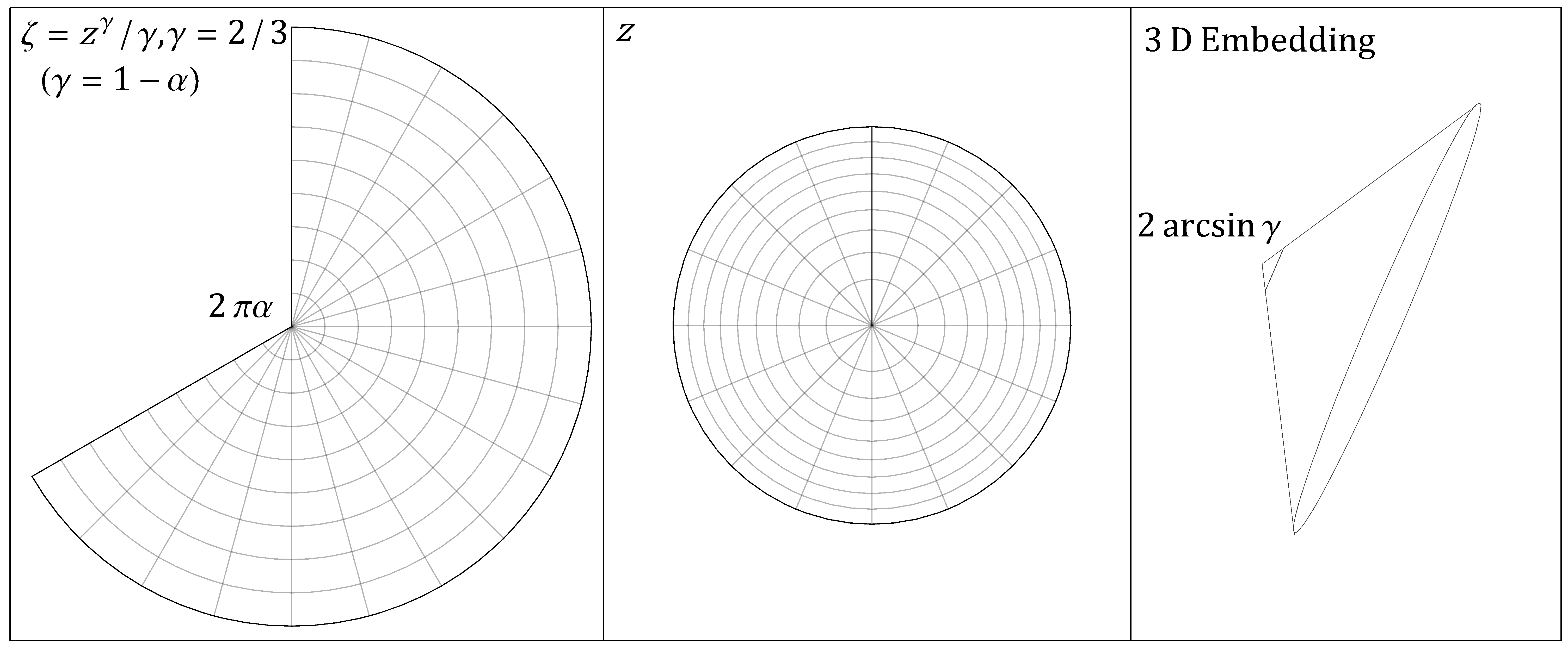
Figure 1: Schematic diagram of a cone and its 3D embedding

Let denote the complex coordinate on the plane as $\xi$ and the cone angle $2\pi\gamma=2\pi(1-\alpha)$. The wedge is a domain $0\leq{\rm arg}\,\xi<2\pi\gamma$ with the Euclidean metric $ds^{2}=|d\xi|^{2}$. A pullback of a singular conformal map

$$z\to\xi(z)=(z-z_{0})^{\gamma}/\gamma$$ (23)

maps the wedge to a punctured disk. The map introduces the complex coordinates $(z,\bar{z})$ where the metric is conformal

$$ds^{2}=|z-z_{0}|^{-2\alpha}|dz|^{2}.$$ (24)

The quantum mechanics on the cone assumes the ‘wedge-periodic’ condition. The lowest Landau level on a cone is spanned by the holomorphic polynomials of $z$ (see, (46)) in the metric (24).

Eq. (18) is valid on any genus-zero surface. Specifically, in the neighborhood of the conical singularity the the conformal factor in (18) behaves as (22) and locally the state reads

$$\Psi_{\alpha}\!=\!\prod_{i<k}\!(z_{i}\-\!-\!z_{k})^{\beta}\prod_{i}\!|z_{0}\!-\!z_{i}|^{j\alpha}e^{-{|z_{i}-z_{0}|^{2\gamma}}/({4l^{2}\gamma^{2}})}.$$

Then the generating functional $\mathcal{Z}_{\alpha}$ is the expectation value of this operator.

A singularity can be interpreted as an insertion of the ‘vertex operator’ such that the generating functional $\mathcal{Z}_{\alpha}$ is the expectation value of this operator. We will show that this operator is conformal primary. This means that under a dilatation transformation of the metric close to the singularity, the functional transforms conformally

$$-\delta\log\mathcal{Z}_{\alpha}=\Delta_{\alpha}\delta\phi.$$

Here $\Delta_{\alpha}$ is the conformal dimension. Eq. (21) identifies the conformal dimension with the angular momentum (7). We compute it in the remaining part of the paper.

Calculations are the most convenient in complex notation. We will need the formula for the angular momentum written in complex coordinates. The momentum in complex coordinates reads $P_{z}dz+P_{\bar{z}}d\bar{z}=\ P_{\xi}d\xi+P_{\bar{\xi}}d\bar{\xi}$ in local coordinates related by the conformal map (23). Then with the help of (23), the angular momentum density in flat coordinates reads ${\rm Im}(\xi P_{\xi})={\rm Im}(\xi\frac{dz}{d\xi}P_{z})=\gamma^{-1}{\rm Im}(zP_{z})$. Hence

$$\mathrm{L}=-\gamma^{-1}\int{\rm Im}(zP_{z})\,dV.$$ (25)

Conformal Ward identity Moments of the density and the angular momentum are computed via the Ward identity. The Ward identity reflects the invariance of the integral (19) under the infinitesimal holomorphic change of variables $z_{i}\to z_{i}+\epsilon/(z-z_{i})$. It claims that the function of coordinates $z_{i}$ and a complex parameter $z$

$$\!\sum_{i}\frac{\partial_{z_{i}}Q+(1\!-\!j)\partial_{z_{i}}\phi}{z-z_{i}}\!+\frac{\beta}{2}\left(\sum_{i}\frac{1}{z-z_{i}}\right)^{2}\!+\!\sum_{i}\frac{1-\frac{\beta}{2}}{(z-z_{i})^{2}}$$

vanishes under averaging over the state.

The identity is closely related to the Ward identity of conformal field theory. In order to flesh out this analogy, we introduce the scalar field $\varphi$

$$\varphi=-2\beta\sum_{i}\log|z-z_{i}|-Q.$$ (26)

We also need the holomorphic component of the conformal ‘stress tensor’

$$T=\frac{\nu}{2}\langle\left(\partial_{z}\varphi\right)^{2}\rangle-\mu_{H}\langle\partial_{z}^{2}\varphi\rangle.$$ (27)

Then the Ward identity can be brought to the form connecting the momentum and the conformal ‘stress tensor’

$$\frac{1}{\hbar}\int\frac{{\rm{i}}P_{z^{\prime}}-\frac{\mu_{H}}{2\pi}\partial_{z^{\prime}}(eB)}{z-z^{\prime}}dV_{z^{\prime}}=T.$$ (28)

We describe the algebra elsewhere.

Trace of the conformal stress tensor The meaning of the Ward identity becomes transparent if we complete the stress tensor by its trace $\Theta$, defined through the conservation law equation

$$\partial_{\bar{z}}T+e^{\phi}\partial_{z}\Theta=0.$$ (29)

Together the components $T,\,\bar{T},\,\Theta$ form a quadratic differential $T_{ij}dx^{i}dx^{j}=T(dz)^{2}+\bar{T}(d\bar{z})^{2}+2e^{\phi}\Theta dzd\bar{z}$. Then $\partial_{\bar{z}}$ derivative brings (28) to the form

$$P_{z}=\frac{1}{2\pi{\rm{i}}}\partial_{z}\left(\mu_{H}(eB)-2\hbar\Theta\right).$$ (30)

The formula (30) identifies the trace $\Theta$ with the intensive part of the angular momentum

$${\mathrm{L}=-\frac{\mu_{H}}{2\pi\gamma}\int(eB)dV}+\frac{\hbar}{\pi\gamma}\int\Theta\,dV.$$

Gravitational Anomaly On its own, the Ward identity is a relation between one and two-point correlation functions. The two-point function $\langle(\partial_{z}\varphi)^{2}\rangle$ in the Ward identity is evaluated coincident points. The connected part of this function $T^{A}=\frac{\nu}{2}\langle(\partial_{z}\varphi)^{2}\rangle_{c}=\frac{\nu}{2}\left[\langle(\partial_{z}\varphi)^{2}\rangle-\langle\partial_{z}\varphi\rangle^{2}\right]$ is the entry which converts the identity into a meaningful equation. In Can et al. (2014) it was argued that the connected two-point function is proportional to the Schwarzian of the metric

$$T^{A}=\frac{1}{12}\mathcal{S}[\phi],\quad\mathcal{S}[\phi]\equiv-\frac{1}{2}(\partial_{z}\phi)^{2}+\partial_{z}^{2}\phi.$$ (31)

Thus $T=T^{C}+T^{A}$ consists of the ‘classical’ part

$$T^{C}=\frac{\nu}{2}\left(\langle\partial_{z}\varphi\rangle\right)^{2}-\mu_{H}\partial_{z}^{2}\langle\varphi\rangle$$ (32)

and the anomalous part (31). This explicit representation of $T$ converts the Ward identity to the equation.

This equation consists of terms of a different order in magnetic length and has to be solved iteratively. The leading approximation, where $\langle\rho\rangle\approx\bar{\rho}$ suffices. From (26) it follows that $\langle\varphi\rangle\approx(\mu_{H}/\nu)\phi$. Up to this order the classical part of the stress tensor is $T^{C}=-(\mu_{H}^{2}/\nu)\left[-\frac{1}{2}(\partial_{z}\phi)^{2}+\partial_{z}^{2}\phi\right]$. Together with the anomalous part (31) the stress tensor reads

$$T=\frac{c_{H}}{12}\mathcal{S}[\phi].$$ (33)

On smooth surfaces by virtue of (29)

$$\Theta=\frac{c_{H}}{48}R.$$

This is the trace anomaly.

Thus, to leading order the Ward identity is equivalent to the conformal Ward identity. Eq. (30) then yields the result obtained in Klevtsov and Wiegmann (2015) for the momentum on a smooth surface

$$P_{z}=\frac{1}{2\pi{\rm{i}}}\partial_{z}\left(\mu_{H}\,(eB)-\hbar\frac{c_{H}}{24}R\right).$$ (34)

In its turn it yields the angular momentum given by (1). For reference we present the formula for the density on a smooth surface, which follows from (34) and (16). It was previously obtained in Can et al. (2015)

$$\rho=\!\bar{\rho}\!+\!\frac{1}{4\pi B}\left[(\nu\!-\!\frac{1}{2})\Delta B\!+\!\left((1\!-\!j)\frac{\mu_{H}}{2}\!+\!\frac{c_{H}}{24}\right)\frac{\hbar}{e}\!\Delta R\right].$$

Geometric singularity On a singular surface the formula (34) is not valid, since the curvature is singular. However, the results promptly follow from the dilatation sum rule we now obtain.

We multiply (28) by $\frac{zdz}{2\pi{\rm{i}}}$ and integrate it along a boundary of an infinitesemaly small parcel. Using $\frac{1}{2\pi{\rm{i}}}\oint\frac{zdz}{z-z^{\prime}}=z^{\prime}$, (25) we reduce the Ward identity to the sum rule for the intensive part of the angular momentum

$$\gamma\mathrm{L}_{\alpha,a}=\hbar\,\oint T(z)\frac{zdz}{2\pi{\rm{i}}}.$$ (35)

and notice that in the neighborhood of singularity $T(z)$ is a holomorphic function. Thus $\oint T(z)\frac{zdz}{2\pi{\rm{i}}}={\rm res}(zT)$.

We compute the singular part of the stress tensor by evaluating the Schwarz derivative on the singular metric (22). Equivalently, we treat a conical singularity as a conformal map (23) and compute the Schwarz derivative of the map

$$\mathcal{S}[\phi]\equiv\{\xi,\,z\}=\frac{\xi^{\prime\prime\prime}}{\xi^{\prime}}-\frac{3}{2}\left(\frac{\xi^{\prime\prime}}{\xi^{\prime}}\right)^{2}=\frac{\alpha(2-\alpha)}{2z^{2}}.$$

We obtain

$$T=\frac{c_{H}}{24}\frac{\alpha(2-\alpha)}{z^{2}}.{}$$ (36)

Using (35), we arrive at our main result (7).

Magnetic singularity In this case, the gravitational anomaly does not contribute to the the singularity of the the stress tensor. Rather, the stress tensor receives an additional contribution from the magnetic potential of the flux tube $Q_{a}=2a\log|z|$

$$T=-\frac{\nu}{2}(\partial_{z}Q_{a})^{2}-\mu_{H}\partial_{z}^{2}Q_{a}=\frac{h_{a}}{z^{2}},$$ (37)

where $h_{a}$ is the conformal dimension (5).

Finally, when the flux tube sits on top of a conical singularity, the stress tensor is the sum of (37) and (36). Near the singularity $T\sim(\gamma\Delta_{\alpha}+h_{a})/z^{2}$. This implies the relation (8).

Exchange statistics Now consider adiabatically exchanging two singularities. The state will acquire a phase. Since the state is a holomorphic function of singularity position, its holonomy is encoded in the normalization factor. The phase is then $\Phi_{12}=\frac{{\rm{i}}}{2}\oint d\log\mathcal{Z}$, where the integral in positions of singularities goes along the adiabatic path. The adiabatic connection $d\log\mathcal{Z}$ treated as a differential of the position, say, the first singularity has a pole when two singularities coincide, so the phase is the residue of the pole $\Phi_{12}=-\pi\,{\rm res}[d\log\mathcal{Z}]$.

For conical singularities, the residue arises entirely from the gravitational anomaly. We notice that the calculation of the normalization factor for multiple singularities is closely related to the determinant of the Laplacian ${\rm Det(-\Delta)}$ on singular surfaces. This relation was discussed in Can et al. (2015); Laskin et al. (2015); Klevtsov and Wiegmann (2015). A reason for this is that the stress tensor for $\log\mathcal{Z}$ and $\frac{1}{2}c_{H}\log{\rm Det}(-\Delta)$, share the same singularities.

The result is summarized by the formula

$$\log\mathcal{Z}|_{p_{1}\to p_{2}}=\frac{c_{H}}{12}\alpha_{1}\alpha_{2}\left(\frac{1}{\gamma_{1}}+\frac{1}{\gamma_{2}}\right)\log|p_{1}-p_{2}|.$$ (38)

where $p_{1}$ and $p_{2}$ are positions of two merging singularities.

Then the adiabatic connection is

$$d\log\mathcal{Z}=\frac{c_{H}}{24}\alpha_{1}\alpha_{2}\left(\frac{1}{\gamma_{1}}+\frac{1}{\gamma_{2}}\right)\frac{dp_{1}-dp_{2}}{p_{1}-p_{2}}.$$ (39)

It prompts the formula (10) for the exchange statistics.

We illustrate the calculation of the generating functional on the example of a genus-0 polyhedral surface, such as a cube, tetrahedral, etc., whose vertices are separated by distances well exceeding the magnetic length. In this calculation we focus on the geometric singularities setting the fluxes $a=0$. The metric describing a polyhedron is piece-wise flat with multiple conical singularities. It is obtained from the Schwarz-Christoffel map $\xi(z)$ unfolding the polyhedron

$$e^{\phi}=|{\xi(z)}^{\prime}|^{2}=\prod_{i}|z-p_{i}|^{-2\alpha_{i}}.$$ (40)

The metric describes a flat surface with conical singularities of the order $\alpha_{i}$, conditioned by the Gauss-Bonnet theorem $-\sum_{i}\alpha_{i}+2=0$, and located at points $p_{i}$. The magnetic potential $-\hbar\Delta Q=2eB$ corresponding to a uniform magnetic field will be $Q=-|\xi(z)|^{2}/2l^{2}$.

The Schwarzian of this metric is

$$\mathcal{S}[\phi]=\sum_{i}\frac{-\frac{1}{2}\alpha_{i}^{2}+\alpha_{i}}{(z-p_{i})^{2}}+\frac{\gamma_{i}}{z-p_{i}},\quad\gamma_{i}\equiv-\sum_{j\neq i}\frac{\alpha_{i}\alpha_{j}}{p_{i}-p_{j}}.$$

Using the explicit form of the metric, we find the following asymptotic behavior of the magnetic potential and the metric at singularities

$$\partial_{p_{i}}\phi|_{z\to p_{i}} =-\partial_{z}\phi+\frac{\gamma_{i}}{\alpha_{i}}+...,$$

$$\partial_{p_{i}}\phi|_{z=p_{j}} =-\frac{\alpha_{i}}{p_{i}-p_{j}},$$

$$\partial_{p_{i}}Q|_{z\to p_{i}} =(-\partial_{z}+\frac{\gamma_{i}}{\alpha_{i}})Q|_{z\to p_{i}}+...,$$ (41)

$$\partial_{p_{i}}Q|_{z=p_{j}} =-\frac{\alpha_{i}}{p_{i}-p_{j}}Q|_{z=p_{j}}$$

Next, we use the formula for the angular momentum of a that for a single cone (7), which we write in the form

$$\int_{D_{\epsilon}(p_{i})}\left(-Q+(j-1)\right)\left(\rho-\rho_{\infty}\right)dV =\Delta_{\alpha_{i}}.$$ (42)

To make sense of this formula for multiple cones, we take the domain of integration $D_{\epsilon}(p_{i})$ to be a small disk of radius $\epsilon$ centered on $p_{i}$ which is much larger than the magnetic length but much smaller than the Euclidean distance to the closest neighboring cone point. In this case, $\rho_{\infty}=\frac{\nu}{2\pi l^{2}}$ is the density far from any cone points.

For multiple cones, there is also another important non-vanishing sum rule that comes from the examining the simple poles of the Ward identity, which come entirely from the Schwarzian of the metric. This sum rule reads

$$\int_{D_{\epsilon}(p_{i})}\partial_{z}\left(Q+(1-j)\phi\right)\left(\rho-\rho_{\infty}\right)dV=-\frac{c_{H}}{12}\gamma_{i}.$$ (43)

The proof for these sum rules comes directly from the Ward identity (28) specified for a uniform magnetic field

$$\frac{1}{\hbar}\int\frac{i\langle P_{z^{\prime}}\rangle}{z-z^{\prime}}dV_{z^{\prime}}=\langle T\rangle=\frac{c_{H}}{12}\mathcal{S}[\phi]+O(l^{2}).$$ (44)

Since the RHS is proportional to the Schwarzian, it will have second order pole and simple poles at the cone points. This implies that the integral on the LHS has a Laurent expansion around each cone point. Comparing the residues of the poles, we find (42) comes from the second order pole of the Schwarzian, whereas (43) follows from the simple pole.

Now we are equipped to derive the variational formula for the generating functional.

Derivatives with respect to the cone points will act only the single-particle factors of the wave function (18), and thus lead to

$$\partial_{p_{i}}\log Z =\int\partial_{p_{i}}\left(Q+(1-j)\phi\right)\rho)dV.$$ (45)

In the integrand we write $\rho=(\rho-\rho_{\infty})+\rho_{\infty}$. The contribution of $\rho_{\infty}$ is of the order $l^{-2}$. We ignore it and focus on the contribution of $\rho-\rho_{\infty}$ which has a finite support at the conical singularity points $p_{i}$. Therefore, we convert the integral over the entire surface to a sum of integrals over small disks $D_{\epsilon}(p_{j})$ centered on singularities

$$\partial_{p_{i}}\log Z=\sum_{j}\int_{D_{\epsilon}(p_{j})}\partial_{p_{i}}\left(Q+(1-j)\phi\right)\left(\rho-\rho_{\infty}\right)dV.$$

With this, we utilize the asymptotic expressions for $Q$ and $\phi$ in (41), combined with the formula (42) for the moment of inertia and the sum rule (43). We obtain

$$\partial_{p_{i}}\log Z =\frac{c_{H}}{12}\gamma_{i}-\frac{\gamma_{i}}{\alpha_{i}}\Delta_{\alpha_{i}}+\sum_{j\neq i}\left(\frac{\alpha_{i}}{p_{i}-p_{j}}\right)\Delta_{\alpha_{j}}$$

$$=\frac{c_{H}}{24}\sum_{j\neq i}\frac{\alpha_{i}\alpha_{j}}{p_{i}-p_{j}}\left[\frac{1}{\gamma_{i}}+\frac{1}{\gamma_{j}}\right].$$

This formula represents the adiabatic connection with respect to adiabatic displacement of conical singularity announced in the main text in Eq (30).

Integer QH-state on a cone The formulae for the charge of the singularity (14) and the moment of inertia (15) are readily checked against the direct calculations for the integer case $\nu=1$. See Furtado et al. (1994); *Furtado2; *Poux for a study of Landau levels on a cone. In the case where a flux $(h/e)a$ threads the cone the Landau level is spanned by one-particle states $k=0,\dots,N\!-\!1$

$$\psi_{k}\!=\!\frac{e^{-{|\xi|}^{2}/{4l^{2}}}}{l\sqrt{2\pi\gamma\Gamma(\frac{k}{\gamma}+\frac{q}{\gamma}+1)}}\left(\frac{|\xi|}{\sqrt{2}l}\right)^{\frac{q}{\gamma}}\cdot\left(\!\!\frac{\xi}{\sqrt{2}l}\!\right)^{\frac{k}{\gamma}},$$ (46)

where $q=a+\alpha j$, and the density is the sum of densities of each one-particle state

$$\rho=\sum_{k=0}^{N-1}|\psi_{k}|^{2}.$$ (47)

We observe that in the integer case the magnetic singularity and spin come together in a combination $q=a+\alpha j$.

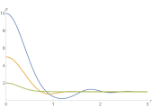
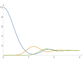
Figure 2: Left panel: Density on a cone of angle $\gamma=1/10,1/5,1/2$ (blue, yellow, green) with spin $j=0$. Right panel: Density on a cone of angle $\gamma=1/10$ and spin $j=0,1/2,1$ (blue, yellow, green).

At $N\to\infty$ the density is expressed in terms of Mittag-Leffler function

$$\rho=\rho_{\infty}\gamma^{-1}e^{-x}x^{\frac{q}{\gamma}}E_{\frac{1}{\gamma},\frac{q}{\gamma}+1}\left(x^{\frac{1}{\gamma}}\right),$$

where we denoted $x=|\xi|^{2}/2l^{2}$, and $\rho_{\infty}=1/2\pi l^{2}$. We recall the definition of the Mittag-Leffler function

$$E_{a,b}(z)=\sum_{k\geq 0}\frac{z^{k}}{\Gamma(ak+b)}.$$

We find the moments from the arguments used to obtain the conformal Ward identity. Under re-scaling the magnetic length $l^{2}\to\lambda^{-1}l^{2}$ the state (46) scales

$$\psi_{k}\to\lambda^{\frac{1}{2}+\frac{k+q}{2\gamma}}e^{(1-\lambda){|\xi|}^{2}/{4l^{2}}}\psi_{k}.$$

but remains normalized. The normalization condition for the new state yields the identity

$$\int e^{(1-\lambda)\frac{|\xi|^{2}}{2l^{2}}}|\psi_{k}|^{2}dV=\lambda^{-1-(q+k)/\gamma}.$$

Then, summing over all modes and taking $N\to\infty$ at $|\lambda|>1$ we obtain the exact Laplace transform of the density

$$\int e^{(1-\lambda)\frac{|\xi|^{2}}{2l^{2}}}(\rho-\rho_{\infty})dV =\frac{\lambda^{-1-\frac{q}{\gamma}}}{1-\lambda^{-1/\gamma}}-\frac{\gamma}{\lambda-1}$$

$$=\frac{\lambda^{\frac{\alpha-2}{2\gamma}+\frac{m_{0}}{\gamma}}}{1-\lambda^{-1/\gamma}}-\frac{\gamma}{\lambda-1}$$

where $m_{0}=-a+(1-2j)\alpha/2$ is the charge of the cone. This formula can be seen as a generating function of moments (12). Expanding around $\lambda=1$ yields the charge $m_{0}$ (14) and the moment of inertia $m_{2}$ (15).

In the orbifold setting the density is a finite sum not where $\gamma(s,x)=\int_{0}^{x}t^{s-1}e^{-t}dt$ is the lower incomplete gamma function. At $\gamma=1/n$ and $q=0$, the density is Riccati’s generalized hyperbolic function - the sum over $n$-roots of unity $\omega^{k}_{n}=e^{{\rm{i}}\frac{2k\pi}{n}}$

$$\rho=\rho_{\infty}e^{-x}\sum_{k=0}^{n-1}\exp\left(\omega_{n}^{k}x\right)$$

In Fig.2, we illustrate how the cone angle and spin affect the density, respectively. In both figures, the density far away from the singularity is normalized to $1$ and the distance to the conical point is measured in units of magnetic length. On the left panel we set $j=0$ and plot $\rho$ for $\gamma=1/2,1/5,1/10$. The values of density near the origin reflect the charge $m_{0}$ accumulated at the tip of the cone and feature oscillations on the order of magnetic length away from the apex. We comment that magnetic singularity does not feature oscillations at $\nu=1$. On the right panel we set $\gamma=1/10$ and show the effect of spin at $j=0,1/2,2$. Unless spin is zero the charge $m_{0}$ is negative. The cone repels electrons. Spin also suppresses oscillations, but for small values of spin oscillations persist. For larger values of spin (not plotted) oscillations are suppressed entirely.

Apart from the flat cone, there exist exact results for the “American football” geometry, Fig. 3, a unique surface with positive constant curvature and two conical singularities Troyanov (1989). The singularities have the same order and antipodal. The football metric reads

$$ds^{2}=\frac{(1-\alpha)^{2}|z|^{-2\alpha}}{\left(1+|z|^{2\gamma}/4r^{2}\right)^{2}}|dz|^{2},\quad\gamma=1-\alpha.$$ (48)

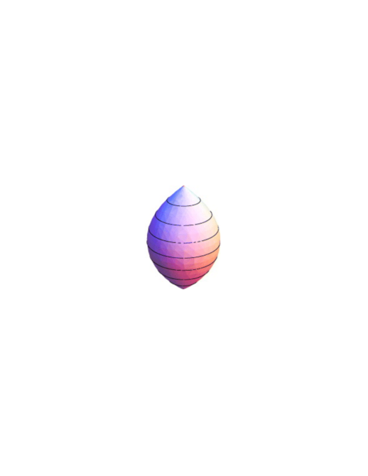
Figure 3: “American football”: a surface of constant positive curvature and two antipodal conical singularities

The volume and the curvature of this surface are
$V=4\pi r^{2}\gamma$ and $R=2/r^{2}$, respectively. Identical conical singularities of order $\alpha$ are located at $z=0$ and $z=\infty$. The number of states is $N=N_{\Phi}+(1-2j)-2a$, where $N_{\Phi}$, is the total magnetic flux, $a$ is the flux threaded through the singularities, and

$$\rho_{\infty}=\frac{e}{h}B+\frac{(1-2j)}{8\pi}\frac{2}{r^{2}},$$

is the bulk density away from the conical singularities.

In coordinates $\xi=z^{\gamma}/(2r\gamma)$, the normalized eigenstates are

$$\psi_{k} =\frac{1}{\sqrt{V\mathcal{N}_{k}}}\frac{\xi^{\frac{1}{\gamma}(k+q)}}{(1+|\xi|^{2})^{\frac{1}{2\gamma}{N}_{\Phi}-j}},\quad q=a+\alpha j,$$

where the normalization factor is

$$\mathcal{N}_{k} =B\left(\frac{1}{\gamma}N_{\Phi}-2j+1-\frac{1}{\gamma}{(k+q)},\frac{1}{\gamma}{(k+q)}+1\right)$$

and $B(x,y)=\Gamma(x)\Gamma(y)/\Gamma(x+y)$ is the beta-function. The formula (47) gives the density

$$\rho= \rho_{\infty}\gamma^{-1}(1+|\xi|^{2})^{-2(N_{\Phi}/\gamma-2j)}\times$$

$$\sum_{k=0}^{N-1}\frac{\Gamma(N_{\Phi}/\gamma-2j+1)|\xi|^{\frac{2}{\gamma}(k+q)}}{\Gamma(N_{\Phi}/\gamma-2j+1-(k+q)/\gamma)\Gamma((k+q)/\gamma+1)}.$$ (49)

As before, the density simplifies when $q=0$ and $\gamma^{-1}=n$ is integer. Writing as before the $n^{th}$ root of unity $\omega_{n}=e^{{\rm{i}}2\pi/n}$, we find

$$\rho=\rho_{\infty}\left(1+|\xi|^{2}\right)^{-nN_{\Phi}}\sum_{k=0}^{n-1}\left(1+\omega_{n}^{k}|\xi|^{2}\right)^{nN_{\Phi}}.$$ (50)

The charge moment follows from simple integration

$$m_{0} =\int\left(\langle\rho\rangle-\rho_{\infty}\right)dV=N-N_{\Phi}+(1-2j)(1-\alpha)$$

$$=-(1-2j)\alpha-2a.$$

This is twice the charge of a single flat cone given by (14).

We thank A. Abanov, R. Biswas, S. Ganeshan, A. Gromov, S. Klevtsov, J. Ross, J. Simon, D. T. Son, A. Waldron, and S. Zelditch for illuminating discussions. The work was supported in part by the NSF under the Grants NSF DMR-1206648, NSF DMR-MRSEC 1420709, and NSF PHY11-25915.

References

- Avron et al. (1995) J. E. Avron, R. Seiler, and P. G. Zograf, Phys. Rev. Lett. 75, 697 (1995).
- Lévay (1995) P. Lévay, J. Math. Phys. 36, 2792 (1995).
- Lévay (1997) P. Lévay, Phys. Rev. E 56, 6173 (1997).
- Wen and Zee (1992) X. G. Wen and A. Zee, Phys. Rev. Lett. 69, 953 (1992).
- Fröhlich and Studer (1992) J. Fröhlich and U. M. Studer, Commun. Math. Phys. 148, 553 (1992).
- Hoyos and Son (2012) C. Hoyos and D. T. Son, Phys. Rev. Lett. 108, 066805 (2012), arXiv:1109.2651.
- Read (2009) N. Read, Phys. Rev. B 79, 045308 (2009), arXiv:0805.2507v3.
- Read and Rezayi (2011) N. Read and E. H. Rezayi, Phys. Rev. B 84, 085316 (2011), arXiv:1008.0210.
- Douglas and Klevtsov (2009) M. R. Douglas and S. Klevtsov, Commun. Math. Phys. 293, 205 (2009), arXiv:0808.2451v1.
- Klevtsov (2014) S. Klevtsov, J. High Energy Phys. 2014, 1 (2014), arXiv:1309.7333v2.
- Can et al. (2014) T. Can, M. Laskin, and P. Wiegmann, Phys. Rev. Lett. 113, 046803 (2014), arXiv:1402.1531v2.
- Can et al. (2015) T. Can, M. Laskin, and P. B. Wiegmann, Ann. Phys. 362, 752 (2015), arXiv:1411.3105v3.
- Abanov and Gromov (2014) A. G. Abanov and A. Gromov, Phys. Rev. B 90, 014435 (2014), arXiv:1401.3703v1.
- Gromov and Abanov (2014) A. Gromov and A. G. Abanov, Phys. Rev. Lett. 113, 266802 (2014), arXiv:1403.5809v1.
- Gromov et al. (2015) A. Gromov, G. Y. Cho, Y. You, A. G. Abanov, and E. Fradkin, Phys. Rev. Lett. 114, 016805 (2015), arXiv:1410.6812v3.
- Laskin et al. (2015) M. Laskin, T. Can, and P. Wiegmann, Phys. Rev. B 92, 235141 (2015), arXiv:1412.8716v2.
- Ferrari and Klevtsov (2014) F. Ferrari and S. Klevtsov, J. High Energy Phys. 2014, 1 (2014), arXiv:1410.6802v3.
- Bradlyn and Read (2015) B. Bradlyn and N. Read, Phys. Rev. B 91, 165306 (2015), arXiv:1502.04126v2.
- Klevtsov and Wiegmann (2015) S. Klevtsov and P. Wiegmann, Phys. Rev. Lett. 115, 086801 (2015), arXiv:1504.07198v2.
- Vafa (2015) C. Vafa, (2015), arXiv:1511.03372v3, arXiv:1511.03372 [cond-mat.mes-Hall] .
- Katanaev and Volovich (1992) M. Katanaev and I. Volovich, Ann. Phys. 216, 1 (1992).
- Lammert and Crespi (2004) P. E. Lammert and V. H. Crespi, Phys. Rev. B 69, 035406 (2004).
- Vozmediano et al. (2010) M. Vozmediano, M. Katsnelson, and F. Guinea, Phys. Rep. 496, 109 (2010).
- Schine et al. (2015) N. Schine, A. Ryou, A. Gromov, A. Sommer, and J. Simon, (2015), arXiv:1511.07381v1, arXiv:1511.07381 [cond-mat.quant-gas] .
- Troyanov (1989) M. Troyanov, Lecture Notes in Math 1410, 296 (1989).
- Troyanov (2007) M. Troyanov, IRMA Lectures in Math. and Theor. Phys. 11, 507 (2007), arXiv:1504.07198.
- Thurston (1998) W. P. Thurston, Geom. Topol. Monogr. 1, 511 (1998), arXiv:math/9801088v2, math/9801088 .
- Takhtajan and Zograf (2002) L. Takhtajan and P. Zograf, Trans. Amer. Math. Soc. 355, 1857 (2002), arXiv:math/0112170.
- Knizhnik (1987) V. G. Knizhnik, Commun. Math. Phys. 112, 567 (1987).
- Bershadsky and Radul (1987) M. Bershadsky and A. Radul, Int. J. Mod. Phys. A2, 165 (1987).
- Kvorning (2013) T. Kvorning, Phys. Rev. B 87, 195131 (2013), arXiv:1302.3808v2, arXiv:1302.3808 [cond-mat.str-el] .
- Cardy and Peschel (1988) J. L. Cardy and I. Peschel, Nucl. Phys. B 300, 377 (1988).
- Kokotov (2013) A. Kokotov, Proc. Math. Soc. 141, 725 (2013).
- Aurell and Salomonson (1994) E. Aurell and P. Salomonson, (1994), arXiv:9405140, arXiv:hep-th/9405140 [hep-th] .
- Arovas et al. (1984) D. Arovas, J. R. Schrieffer, and F. Wilczek, Phys. Rev. Lett. 53, 722 (1984).
- Biswas and Son (2014) R. R. Biswas and D. T. Son, (2014), arXiv:1412.3809v1, arXiv:1412.3809 [cond-mat.mes-Hall] .
- Wiegmann (2013a) P. Wiegmann, J. Exp. Theor. Phys. 117, 538 (2013a), arXiv:1305.6893v2.
- Wiegmann (2012) P. Wiegmann, (2012), arXiv:1211.5132v1, arXiv:1211.5132 [cond-mat.str-el] .
- Wiegmann (2013b) P. B. Wiegmann, Phys. Rev. B 88, 241305 (2013b), arXiv:1309.5992v1.
- Laughlin (1981) R. B. Laughlin, Phys. Rev. B 23, 5632 (1981).
- Zabrodin and Wiegmann (2006) A. Zabrodin and P. Wiegmann, J. Phys. A: Math. Gen. 39, 8933 (2006), arXiv:0601009v3, hep-th/0601009 .
- Furtado et al. (1994) C. Furtado, B. G. da Cunha, F. Moraes, E. de Mello, and V. Bezzerra, Phys. Lett. A 195, 90 (1994).
- Marques et al. (2001) G. d. A. Marques, C. Furtado, V. B. Bezerra, and F. Moraes, J. Phys. A: Math. Gen. 34, 5945 (2001), arXiv:quant-ph/0012146v1, quant-ph/0012146 .
- Poux et al. (2014) A. Poux, L. R. S. Araújo, C. Filgueiras, and F. Moraes, Eur. Phys. J. Plus 129, 100 (2014), arXiv:1405.6599, arXiv:1405.6599 [cond-mat.mes-Hall] .
- (45) In a general orbifold setting, where is rational, and , the density is a finite sum where is the lower incomplete gamma function.