Precision Drell-Yan Measurements at the LHC and Implications for the Diphoton Excess

Abstract

Precision measurements of the Drell-Yan (DY) cross sections at the LHC constrain new physics scenarios that involve new states with electroweak (EW) charges. We analyze these constraints and apply them to models that can address the LHC diphoton excess at 750 GeV. We confront these findings with LEP EW precision tests and show that DY provides stronger constraints than the LEP data. While 8 TeV data can already probe some parts of the interesting region of parameter space, LHC14 results are expected to cover a substantial part of the relevant terrain. We derive the bounds from the existing data, estimate LHC14 reach and compare them to the bounds one gets from LEP and future FCC-ee precision measurements.

1 Introduction

Recently both ATLAS and CMS reported an excess in the search for diphoton resonances around $M_{\gamma\gamma}\sim 750$ GeV with 3.2 fb^-1 and 2.6 fb^-1 of integrated luminosity at $\sqrt{s}=13$ TeV, respectively. The local (global) significance of the excess is 3.9 ​$\sigma$ (2.3 ​$\sigma$) for the ATLAS data, with the best-fit value for the width of the resonance $\Gamma\sim 45$ GeV ATLAS-CONF-NOTE . CMS reported a local excess with significance of 2.6 ​$\sigma$ at a mass compatible with ATLAS, assuming a narrow width. This significance goes down to 2 ​$\sigma$ if $\Gamma=45$ GeV is assumed CMS:2015dxe . The findings are compatible with searches at $\sqrt{s}=8$ TeV, given that the production cross section of the potential resonance $S$ increases by about a factor of 5 for the larger center-of-mass energy. This is, for example, realized if the resonance with the mass around 750 GeV is produced in gluon-gluon or $b\bar{b}$ fusion Franceschini:2015kwy . Although these hints are by no means decisive and it is possible, that the origin of both is in somewhat unlikely fluctuations of the background, it is very interesting to understand the consequences of interpreting this excess as a true new physics resonance.

The tentative large width, however, poses challenges for model building, hinting to a large number of new states with sizable charges mediating the decay $S\to\gamma\gamma$ in a weakly coupled framework Knapen:2015dap ; Ellis:2015oso ; McDermott:2015sck ; Angelescu:2015uiz ; Gupta:2015zzs ; Bauer:2015boy . This width implies that also the partial width into photons should be sizable, at least of order $2\times 10^{-4}\ M_{S}$, because there are considerable constraints on the relative size of other possible decay channels of $S$ from the 8 TeV data.

The most popular and reasonable realization of the large number of the new states would be vector-like fermions, charged under the electroweak (EW) force. Since these new states have EW production cross section (and, possibly, very difficult decay modes for experimental detection) they can relatively easily evade the direct LHC searches and still be sufficiently light, well below the TeV scale. It has been noticed in several works before, that these new vector like states significantly modify the running of the hypercharge coupling Gu:2015lxj ; Goertz:2015nkp ; Son:2015vfl . This in turn leads to new constraints, originating from the consistency of these models, perturbativity and the scale of the Landau pole, which all have been discussed in detail in the above mentioned references.

Interestingly, on top of these constraints, one can put experimental constraints on the existence of such large number of new vector-like EW states. As we will show in detail, the presence of such vector-like fermions can be indirectly tested by measuring the neutral Drell-Yan (DY) process at the LHC, considering their impact on the running of the hypercharge coupling. We will demonstrate that large portions of the parameter space, relevant for the 750 GeV diphoton resonance, can be probed in a relatively model independent way via the LHC DY production far away from the $Z$-pole.

The idea to explore the running of the EW couplings to probe new EW states was carefully elaborated on in Ref. Alves:2014cda . This paper has shown that the running of EW couplings, $\alpha_{2}$ and $\alpha_{Y}$, can be successfully probed at the LHC14 and at a future 100 TeV collider, putting new limits that are much stronger than one gets from LEP measurements. For example, it is claimed that the high-luminosity LHC will be sensitive to deviations in $\alpha_{2}$ of less than 10% from the SM value at a scale of 2.5 TeV. In this work we take this idea one step further, and show that precisely the same measurements at LHC8 already put meaningful constraints on the models that are explaining the 750 GeV resonance. We show, for example, that for the EW states around 400 GeV, values of $NQ^{2}\sim 60$ (with $N$ being a total multiplicity number and $Q$ the hypercharge) are in tension with the DY data, already reducing the parameter space for the large width interpretation of the 750 GeV resonance. Future measurements at LHC14 will further shed light on the parameter space of the $S$, which will be particularly powerful in the latter case.

Our paper in organized as follow. In Section 2 we present the perturbative model, which might address the 750 GeV LHC diphoton excess. We also discuss the necessity of the new EW states, explain how they affect the LEP measurements (via changing the Y-parameter) and show the LEP bounds. We will see that these bounds are fairly weak. In Section 3 we briefly overview the theory of DY production at the LHC, with an emphasis on the possible change in the cross sections due to new physics which affects the hypercharge coupling running. In Section 4 we describe our statistical procedure, show the bounds that we get from LHC8 and provide the sensitivity projection for LHC14. Here, we also discuss NLO, PDF and other systematic uncertainties. We summarize the implications of our findings on the 750 GeV diphoton resonance and discuss some future developments in Section 5. Finally, we briefly comment on direct searches for the new EW states in Section 6 and conclude. The technical details concerning the simulation of the SM prediction for the DY process are relegated to Appendix A.

2 Toy Model for 750 GeV Excess and EW Precision Tests

2.1 Overview of data and interpretation

If we interpret the LHC data as a signal for a new resonance in the $\gamma\gamma$ channel, the suggested production cross sections are Franceschini:2015kwy

$$\sigma(pp\to S)\times{{\rm BR}}(S\to\gamma\gamma)=(10\pm 3)~{}{\rm fb}\ \ /\ \ (6\pm 3)~{}{\rm fb}$$ (1)

at ATLAS / CMS, respectively. ATLAS data prefers a relatively wide resonance, $\Gamma_{S}/M_{S}\approx 0.06$. It is important to mention that CMS data does not prefer large width, and it is unclear whether the wide resonance assumptions notably improves the overall fit, when the LHC8 and LHC13 data of both experiments is taken into account. For example, it is claimed in Ref. Buckley:2016mbr that narrow width of the resonance is more likely if the Run II information of both ATLAS and CMS is considered, while the preference to large width is merely marginal, when it is combined with the Run I data.

For concreteness we consider the following effective theory for $S$, assuming that $S$ is a scalar and its couplings do not violate CP:

$${\cal L}_{eff}=\frac{e^{2}SF_{\mu\nu}F^{\mu\nu}}{2\Lambda_{\gamma}}+\frac{g_{3}^{2}SG_{\mu\nu}G^{\mu\nu}}{2\Lambda_{g}}~{}.$$ (2)

If $S$ is a pseudoscalar, one essentially gets the same couplings with the obvious replacements $F_{\mu\nu}F^{\mu\nu}\to F_{\mu\nu}\tilde{F}^{\mu\nu}$ and $G_{\mu\nu}G^{\mu\nu}\to G_{\mu\nu}\tilde{G}^{\mu\nu}$. Here we also assumed that the dominant production channel for $S$ is via gluon fusion. Of course this is not the only option, and production from heavy flavors can be even slightly favored by data if LHC8 is taken into account Franceschini:2015kwy .

In a perturbative model, the couplings in Eq. (2) are induced by new states, charged under the EM and strong force, respectively. As we have alluded, we will further study the model, in which these couplings are induced by new vector-like fermions. In principle, one can induce the coupling of $S$ to photons either via introducing new vector like representations under $SU(2)_{L}$, or under hypercharge (or both). For simplicity, we will focus on the latter case and consider $N_{X}$ new vector-like fermions $X_{i},$ $i=1,..,N_{X}$, only charged under hypercharge. Moreover, we assume that they all share the same mass $M_{X_{i}}\equiv M_{X}$, quantum numbers, and couplings. In this case, one easily matches the scale $\Lambda_{\gamma}$ as

$$\Lambda_{\gamma}^{2}=\frac{16\pi^{4}M_{S}^{2}}{(N_{X}Q_{X}^{2})^{2}y^{2}\tau_{X}|\mathcal{S}(\tau_{X})|^{2}}\,,\ \text{with }\Gamma(S\to\gamma\gamma)=\frac{M_{S}^{3}}{80\pi\Lambda_{\gamma}^{2}}\,.$$ (3)

Here, $Q_{X}$ denotes the common hypercharge of the $X_{i}$, $\tau_{X}\equiv 4M_{X}^{2}/M_{S}^{2}$ and, assuming $S$ is a scalar particle,

$$\mathcal{S}(\tau)\equiv 1+(1-\tau)\arctan^{2}\left(\frac{1}{\sqrt{\tau-1}}\right)~{},$$ (4)

while $y$ is the Yukawa coupling between the new scalar resonance and the vector-like states, ${\cal L}\supset ySXX$. The pseudo-scalar case corresponds to the replacement $\mathcal{S}(\tau)\to{\cal P}(\tau)\equiv\arctan^{2}\left(1/\sqrt{\tau-1}\right)$ together with trading $y$ for the pseudo-scalar Yukawa coupling.

What should the number $N_{X}Q_{X}^{2}$ be to match the data? This again depends on our assumptions. If we assume that $S$ is a narrow resonance, one can end up with a fairly small number of exotic vector-like fermions, which will have a relatively limited impact on the DY precision measurements. In this case the only constraint that the data imposes is

$$\frac{\Gamma_{gg}\Gamma_{\gamma\gamma}}{M_{S}\Gamma}\sim 10^{-6}~{},$$ (5)

where we use the short-hand notations, $\Gamma_{\gamma\gamma}\equiv\Gamma(S\rightarrow\gamma\gamma),\Gamma_{gg}\equiv\Gamma(S\rightarrow gg)$.

Dijet searches constrain the width into gluons relatively weakly compared to the observed width into photons, $\Gamma_{gg}\lesssim 1200\ \Gamma_{\gamma\gamma}$. This essentially means that if we assume narrow width, we can saturate $\Gamma\simeq\Gamma_{gg}$ and it can be sufficient to reproduce $\Gamma_{\gamma\gamma}/M_{S}\sim 10^{-6}$. This goal is easy to achieve with only $N_{X}Q_{X}^{2}\sim{\cal O}(5-10)$.

The situation dramatically changes if we try to reproduce the 6% width of the resonance, which is preferred by ATLAS. As the width (into some other particles) grows substantially, one needs to increase the width to photons and is easily driven to $\Gamma_{\gamma\gamma}/M_{S}\gtrsim 10^{-3}$, depending on the dominant decay products $f$ of $S$, due to 8 TeV upper bounds on $\Gamma(S\to f)/\Gamma_{\gamma\gamma}$, scaled to 13 TeV Franceschini:2015kwy . In any case, in the wide width scenario, the generic constraint from 8 TeV data, $\Gamma\lesssim 1500\times\Gamma_{\gamma\gamma}$ (considering standard decay modes), suggests that $\Gamma_{\gamma\gamma}/M_{S}$ cannot be lower than $\sim 10^{-4}$. It is important to mention that this requirement is not unique for gluon fusion production and one gets roughly the same requirements of the partial width into diphotons if heavy flavor production is assumed.

The goal $\Gamma_{\gamma\gamma}/M_{S}\sim 10^{-3}$ is notoriously hard to achieve and it demands sufficiently large $N_{X}Q_{X}^{2}\sim{\cal O}(100-500)$, depending on the masses of the new fermions. These numbers are already big enough to significantly deflect the running of $\alpha_{Y}$ from the SM trajectory, such that the effects are clearly visible in DY production.

2.2 LEP constraints

Before analyzing in detail the bounds that we get from the LHC, we first show the bounds from LEP. The $SU(2)_{L}$-singlet vector-like fermions $X$ with non-zero hypercharge $Y\equiv Q_{X}$ and mass $M_{X}$ contribute to the two-point function, $\Pi^{\mu\nu}_{BB}(q^{2})$. Below the mass scale of the heavy fermions, it generates an effective operator $(\partial_{\mu}B^{\mu\nu})^{2}$ which maps on the $\mathcal{Y}$ parameter Barbieri:2004qk ,

$$\mathcal{Y}=d_{X}N_{X}Q_{X}^{2}\,\frac{\alpha_{Y}m_{W}^{2}}{15\pi M_{X}^{2}}~{},$$ (6)

where $d_{X}N_{X}$ denotes the total number of degrees of freedom. The one-loop $\beta$ function of the hypercharge coupling is also encoded in the same two-point function, leading to the same parametric dependence $d_{X}N_{X}Q_{X}^{2}$, and is given by

$$\beta_{g_{1}}^{(1)}=\left(\frac{41}{10}+d_{X}N_{X}Q_{X}^{2}\frac{4}{5}\right)g_{1}^{3}=16\pi^{2}\frac{dg_{1}}{d\ln\mu}~{},$$ (7)

where the modification due to the new vector-like states alters the SM running above the threshold $\mu>M_{X}$. Below the threshold, the heavy fermions $X$ are integrated out and the resulting one-loop $\beta$ function reduces to the SM one.

The best-fit of the $\mathcal{Y}$ parameter from LEP data and the recasted bounds on new vector-like fermions are illustrated in Fig 1. As one would naively expect, these bounds are very weak.

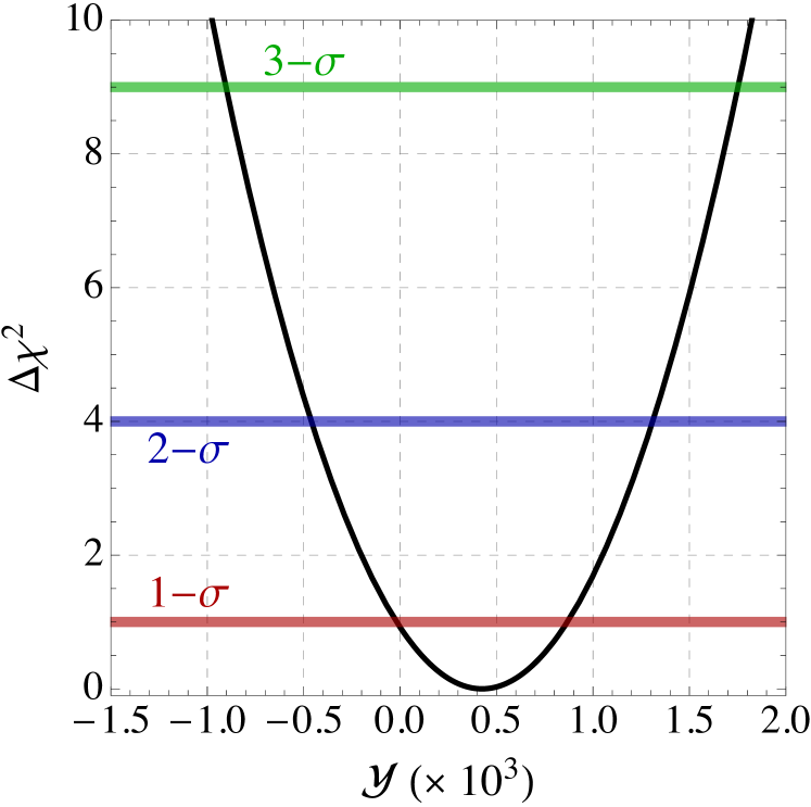
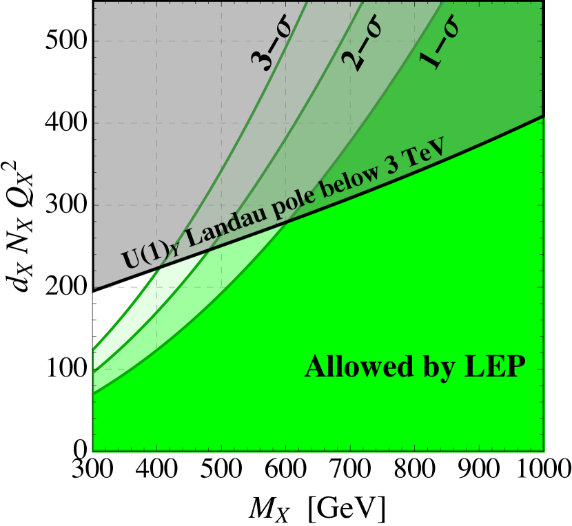
Figure 1: Left panel. One-parameter fit of LEP data in terms of the $\mathcal{Y}$ oblique parameter. All the remaining oblique parameters are set to zero. Right panel. Two-parameter fit of LEP data (allowed region in green) in term of the mass $M_{X}$ of the new vector-like states and the combination $d_{X}N_{X}Q_{X}^{2}$, where $d_{X}$ is the number of degrees of freedom (e.g. $d_{X}=3$ for a color charge). We superimpose (region shaded in gray) the parameter space in which the $U(1)_{Y}$ Landau pole is lowered below $3$ TeV Son:2015vfl .

3 Drell-Yan at the LHC

In this section we show how one can estimate the DY double differential cross section in the presence of the $\alpha_{Y}$ running due to the new physics. The computation of the DY cross section at the LHC proceeds in the following steps.

• At the parton level and in the center of mass partonic reference frame the DY scattering process $q\bar{q}\to Z^{*}/\gamma\to l^{+}l^{-}$ is described by the following double-differential cross-section

  $$\left.\frac{1}{2\,M_{ll}}\frac{d^{2}\hat{\sigma}}{dzdM_{ll}}\right|_{q\bar{q}}=a^{2}f_{q\bar{q}}(s_{W}^{2},M_{ll},z)\times\frac{\pi M_{ll}^{2}}{2}\frac{\delta(\hat{s}-M_{ll}^{2})}{(M_{ll}^{2}-m_{Z}^{2})^{2}+\Gamma_{Z}^{2}m_{Z}^{2}}~{},$$ (8)

  where $z\equiv\cos\theta$, being $\theta$ is the scattering angle in the partonic center of mass frame. The factor $a$ and the rescaling function in Eq. (8), following Alves:2014cda , are defined as

  $$\begin{split}a\equiv&\ \frac{\alpha}{s_{W}^{2}c_{W}^{2}}~{},\\ f_{q\bar{q}}(s_{W}^{2},M_{ll},z)\equiv&\ c_{q\bar{q}}^{(0)}+c_{q\bar{q}}^{(1)}s_{W}^{2}+c_{q\bar{q}}^{(2)}s_{W}^{4}+c_{q\bar{q}}^{(3)}s_{W}^{6}+c_{q\bar{q}}^{(4)}s_{W}^{8}~{}.\end{split}$$ (9)

  The dependence of the scattering cross-section on the running gauge couplings is encoded in $a^{2}f_{q\bar{q}}(s_{W}^{2},M_{ll},z)$ by means of the relations

  $$s_{W}^{2}=\frac{g_{Y}^{2}}{g_{Y}^{2}+g_{L}^{2}}~{},~{}~{}~{}\alpha=\frac{g_{L}^{2}s_{W}^{2}}{4\pi}~{},$$ (10)

  where $g_{L}$ is the $SU(2)_{L}$ gauge coupling with one-loop $\beta$ function $\beta^{(1)}_{g_{L}}=-(19/6)g_{L}^{3}$.

  At this stage it is important to stress that the cross-section in Eq. (8) is derived in full generality with respect to the running of the gauge couplings $g_{Y}$ and $g_{L}$. Since the energy scale of the process is set by $\sqrt{\hat{s}}=M_{ll}$, one has to use the running couplings evaluated at $\mu=M_{ll}$. The impact of new vector-like states with mass $M_{X}$ is captured by solving Eq. (7) with specific values of $d_{X}$, $N_{X}$, $Q_{X}$, and using the corresponding expression for $g_{Y}(\mu=M_{ll})$ in Eqs. (8-10). The SM prediction corresponds to $N_{X}=0$.

  The coefficients $c_{q\bar{q}}^{(i)}$, $i=0,\dots,4$ depend on dilepton invariant mass, quantum numbers of the initial quark-antiquark pair, and scattering angle. We find

  $$c_{q\bar{q}}^{(0)} = \frac{T_{3L}^{2}(1+z)^{2}}{48}~{},$$ (11)

  $$c_{q\bar{q}}^{(1)} = \frac{T_{3L}(1+z)^{2}}{24}\left[(Q_{q}-2T_{3L})-2Q_{q}\frac{m_{Z}^{2}}{M_{ll}^{2}}\right]~{},$$ (12)

  $$c_{q\bar{q}}^{(2)} = \frac{1}{24}\left\{5Q_{q}^{2}(1+z^{2})+4T_{3L}^{2}(1+z^{2})-2Q_{q}T_{3L}[3+z(-2+3z)]\right\}$$

  $$+ \left\{-6Q_{q}(1+z^{2})+T_{3L}[5+z(2+5z)]\right\}\frac{Q_{q}m_{Z}^{2}}{12M_{ll}^{2}}+\frac{Q_{q}^{2}(1+z^{2})}{3}\frac{m_{Z}^{2}(m_{Z}^{2}+\Gamma_{Z}^{2})}{M_{ll}^{4}}~{},$$

  $$c_{q\bar{q}}^{(3)} = \frac{Q(1+z^{2})}{6}\left[(3Q_{q}-2T_{3L})\frac{m_{Z}^{2}}{M_{ll}^{2}}-4Q_{q}\frac{m_{Z}^{2}(m_{Z}^{2}-\Gamma_{Z}^{2})}{M_{ll}^{4}}\right]~{},$$ (14)

  $$c_{q\bar{q}}^{(4)} = \frac{Q_{q}^{2}(1+z^{2})}{3}\frac{m_{Z}^{2}(m_{Z}^{2}+\Gamma_{Z}^{2})}{M_{ll}^{4}}~{},$$ (15)

  where $Q_{u}=2/3$, $T_{3L}=1/2$ ($Q_{d}=-1/3$, $T_{3L}=-1/2$) for, respectively, up- and down-type quarks. At large dilepton invariant mass ($M_{ll}\gg m_{Z}$) $c_{q\bar{q}}^{(3,4)}\to 0$. The scattering cross-section in Eq. (8) is averaged over the initial spin and color. At the weak scale we use the numerical matching values $g_{L}(\mu=m_{Z})=0.649$, $g_{1}(\mu=m_{Z})=0.459$.

• The hadronic differential cross-section is obtained by convoluting with the PDFs

  $$\frac{1}{2\,M_{ll}}\frac{d\sigma}{dM_{ll}}=\int_{0}^{1}dx_{1}dx_{2}dz\sum_{q}\left[f_{q}(x_{1})f_{\bar{q}}(x_{2})+f_{\bar{q}}(x_{1})f_{q}(x_{2})\right]\left.\frac{d^{2}\hat{\sigma}}{dzdM_{ll}^{2}}\right|_{q\bar{q}}~{},$$ (16)

  with $\hat{s}=x_{1}x_{2}s$, being $\sqrt{s}$ the total energy in the hadronic center of mass frame. We introduce the variable $\tau\equiv x_{1}x_{2}$ which corresponds to the fraction of the energy transferred to the partonic system. The rapidity of the lepton is defined as

  $${\rm y}\equiv\frac{1}{2}\log\frac{x_{1}}{x_{2}}~{}.$$ (17)

  The integration over $x_{1}$, $x_{2}$ can be converted to the one over $\tau$, $\rm y$ via the relations,

  $$x_{1,2}=\sqrt{\tau}e^{\pm{\rm y}}~{},~{}~{}~{}~{}~{}dx_{1}dx_{2}=d\tau d{\rm y}~{}.$$ (18)

  Using the identity $\delta(\tau s-M_{ll}^{2})=\delta(\tau-M_{ll}^{2}/s)/s$ we get rid of the integration over $\tau$, and we find

  $$\left.\frac{1}{2\,M_{ll}}\frac{d\sigma}{dM_{ll}}\right|_{\rm th} = \frac{\pi M_{ll}^{2}}{2s}\frac{1}{[(M_{ll}^{2}-m_{Z}^{2})^{2}+\Gamma_{Z}^{2}m_{Z}^{2}]}\int_{-{\rm y}_{\rm max}}^{+{\rm y}_{\rm max}}d{\rm y}\int_{-z_{\rm max}}^{+z_{\rm max}}dz$$ (19)

  $$\times \sum_{q,\bar{q}}f_{q}(\sqrt{\tau}e^{{\rm y}})f_{\bar{q}}(\sqrt{\tau}e^{-{\rm y}})a^{2}f_{q\bar{q}}(s_{W}^{2},M_{ll},z)~{}.$$

  where $z_{\rm max}\equiv\sqrt{1-4p_{\rm T}^{2}/M_{ll}^{2}}$ and ${\rm y}_{\rm max}={\rm min}\{\log(s/M_{ll}^{2})/2,{\rm y}_{\rm cut}\}$; the detector acceptance sets the value ${\rm y}_{\rm cut}=2.5$. The nominal cut on the transverse momentum of the leptons is $p_{\rm T}=25$ GeV. We use the MSTW parton distribution functions at NNLO Martin:2009iq .

• In Eq. (19) the PDF are evaluated setting the renormalization scale at the dynamical value $\mu=M_{ll}$. Furthermore, we make use of the central PDF set. Fixing these two values implies the introduction of both scale and PDF uncertainties in the computation of the theoretical cross-section. We estimate the impact of the scale uncertainty by varying the renormalization scale in $\mu=[1/2\,M_{ll},\,2M_{ll}]$, and we find that it introduces at most $\sim 1\%$ error (see Alves:2014cda for the related discussion). We therefore neglect such correction in our analysis. PDF uncertainty is larger, and can be estimated evaluating the DY cross-section over a statistical sample obtained by changing the PDF eigenvector set in Eq. (19). We include the PDF uncertainty in our analysis, and we refer the reader to section 4 for a detailed discussion.

• Eq. (19) is defined at the LO in the hard scattering process. We include NNLO corrections by properly rescaling—bin by bin in the invariant mass spectrum range—the LO cross-section with respect to the NNLO cross-section, relying on the numerical evaluation of Ref. CMS:2014jea .

We are now ready to compare the theoretical cross-section in Eq. (19) with experimental data extracted from the measurement of the differential DY cross-section in the di-electron and di-muon channels.

4 Analysis and Results

We extract our bounds by means of a simple $\chi^{2}$ analysis derived comparing theory and data. We start defining the $\chi^{2}$ function

$$\chi^{2}(\mathcal{N},N_{eff},M_{X})=\sum_{i,j}\left[\mathcal{N}\left.\frac{d\sigma}{dM_{ll}}\right|_{\rm th}-\left.\frac{d\sigma}{dM_{ll}}\right|_{\rm exp}\right]_{i}\left(\Sigma^{-1}\right)_{ij}\left[\mathcal{N}\left.\frac{d\sigma}{dM_{ll}}\right|_{\rm th}-\left.\frac{d\sigma}{dM_{ll}}\right|_{\rm exp}\right]_{j}~{},$$ (20)

where the sum runs over the invariant mass bins. The theoretical cross-section in Eq. (19) depends on the many free parameters, $d_{X},\,N_{X},\,Q_{X},\,M_{X}$. To simplify the notation we further define $N_{eff}\equiv d_{X}N_{X}Q_{X}^{2}$. We allow for a free overall normalization $\mathcal{N}$ of the theoretical cross-section—over which we marginalize—in order to include possible unknown correlated systematic uncertainties. Denoting with $\chi^{2}_{\rm min}$ the minimum of the function $\chi^{2}(\mathcal{N},N_{eff},M_{X})$, and introducing the marginalized distribution $\chi_{\rm marg}^{2}(N_{eff},M_{X})=\int d\mathcal{N}\chi^{2}(\mathcal{N},\,N_{eff},M_{X})$, we derive confidence level contours by requiring $\chi_{\rm marg}^{2}(N_{eff},M_{X})>\chi^{2}_{\rm min}+\kappa$, with $\kappa=2.30,\,6.18,\,11.83$ at, respectively, $1$-, $2$- and $3\,\sigma$ level.

In Eq. (20) $\left.d\sigma/dM_{ll}\right|_{\rm exp}$ represents the experimentally measured differential cross-section in the dilepton invariant mass while $\Sigma$ is the covariance error matrix. Before we proceed further, we have to distinguish between the analysis at $\sqrt{s}=8$ TeV and $\sqrt{s}=14$ TeV. The reason is that at $\sqrt{s}=8$ TeV we can use data and errors from the DY analysis carried out by CMS in CMS:2014jea . At $\sqrt{s}=14$ TeV, on the contrary, we shall rely on a projection.

4.1 Drell-Yan at $\sqrt{s}=8$ TeV

We use the results of the analysis presented by the CMS collaboration in CMS:2014jea where the differential cross-section in the dilepton invariant mass range $M_{ll}=[15,\,2000]$ GeV was measured using proton-proton collisions at $\sqrt{s}=8$ TeV with an integrated luminosity of $19.7$ fb^-1. Data and errors are publicly available at the website of the Durham HepData Project hepdata_DY .

The covariance error matrix entering in Eq. (20) is given by $\Sigma=\Sigma_{\rm exp}+\Sigma_{\rm PDF}$. $\Sigma_{\rm exp}$ encodes experimental errors (both statistical errors and systematic uncertainties, as discussed in CMS:2014jea ) and correlations related to the pre-FSR invariant mass distribution in the combined dilepton channel CMS:2014jea while $\Sigma_{\rm PDF}$ takes into account the impact of PDF uncertainties in the computation of the differential DY cross-section. We take $\Sigma_{\rm exp}$ from hepdata_DY . The knowledge of the covariance matrix is of fundamental importance since it gives us the possibility to compute the correlation matrix describing correlations between different bins in the invariant mass distribution. The correlation matrix can be written as

$$\mathcal{C}_{\rm exp}=[{\rm diag}(\Sigma_{\rm exp})]^{-1/2}\Sigma_{\rm exp}\,[{\rm diag}(\Sigma_{\rm exp})]^{-1/2}~{}.$$ (21)

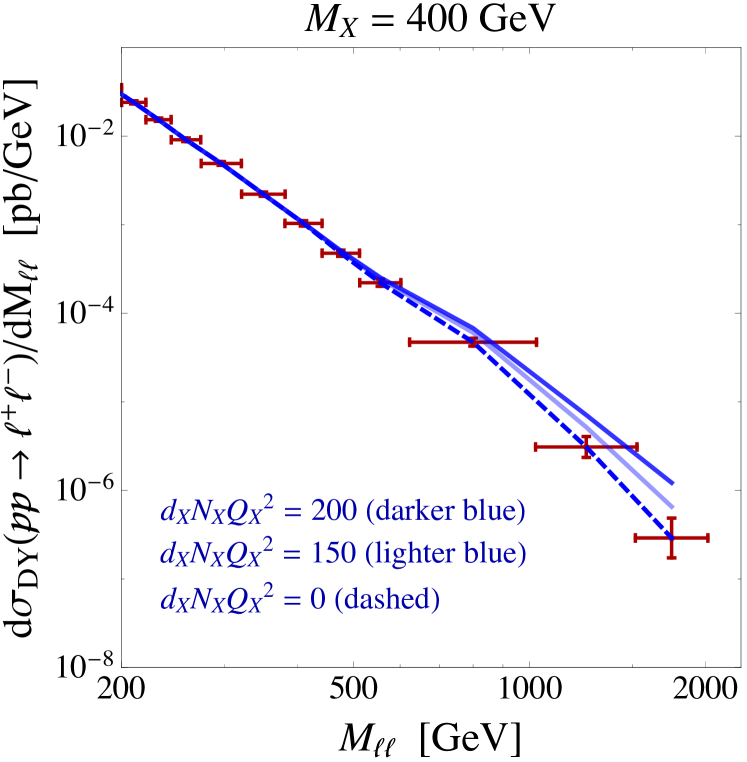
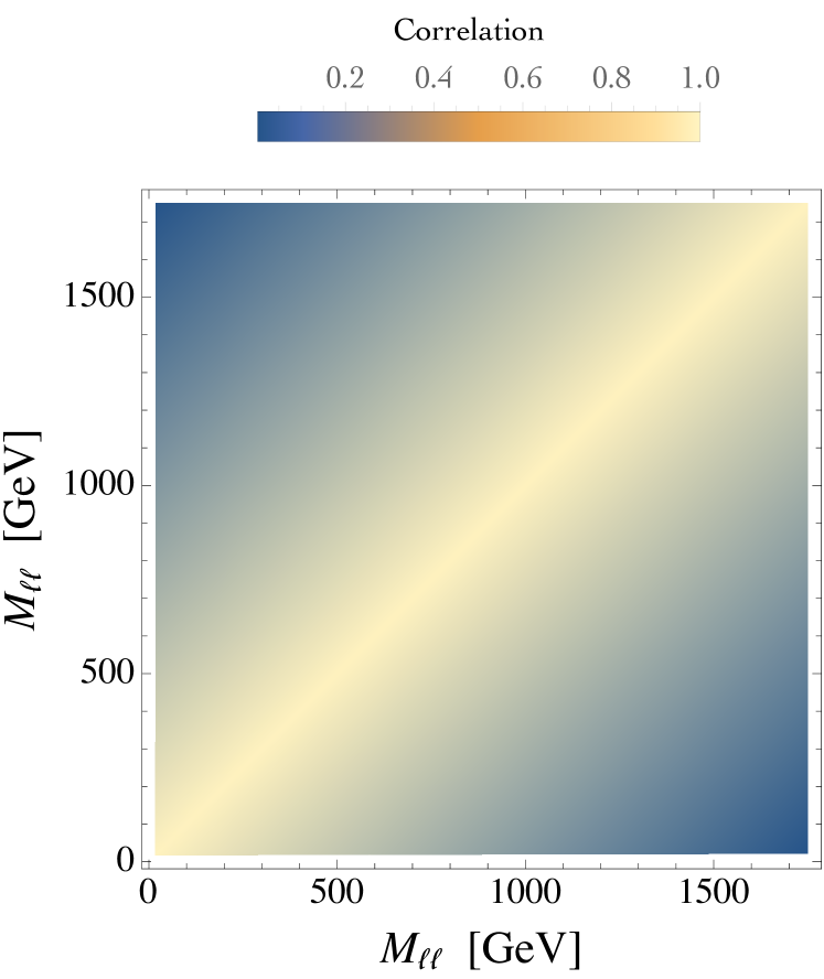
Figure 2: Left panel. Correlation matrix in Eq. (21) derived from the experimental covariance error matrix $\Sigma_{\rm exp}$. Right panel. Comparison between data and theoretical cross-section at large dilepton invariant mass. We show the impact of running couplings for $M_{X}=400$ GeV and different values of the combination $d_{X}N_{X}Q_{X}^{2}$.

In the left panel of Fig. 2 we show the comparison between experimental data and theoretical cross-section at large dilepton invariant mass. We simulated the SM theoretical prediction of the DY fiducial cross section with FEWZ Gavin:2010az and we explain all the details of this simulation, its expected accuracy and comparison with the experimental CMS data in the Appendix. The dashed blue line corresponds to the NNLO SM cross-section, while the blue lines include the extra vector-like fermions. The NNLO SM cross-section is in excellent agreement with the measured values in the whole range of dilepton invariant mass. Let us now discuss the impact of the new vector-like fermions. For illustrative purposes we fix $M_{X}=400$ GeV, and, to better visualize the impact of running couplings, we show two specific cases with $d_{X}N_{X}Q_{X}^{2}=150$ (lighter blue) and $d_{X}N_{X}Q_{X}^{2}=200$ (darker blue). In the dilepton invariant mass range $500\lesssim M_{ll}\lesssim 1000$ GeV the differential cross-section is measured with a $10\%$ accuracy. For $M_{ll}\geqslant M_{X}$ the vector-like fermions actively participate to the hypercharge running, and their impact on the differential cross-section may easily overshoot the data points, as qualitatively shown in Fig. 2, for sufficiently large $d_{X}N_{X}Q_{X}^{2}$. In the right panel of Fig. 2 we show the correlation matrix derived in Eq. (21). As expected, the plot highlights the presence of strong correlations between adjacent bins. The inclusion of the correlation matrix in the $\chi^{2}$ fit plays an important role since it allows to constraint—in addition to the absolute deviation from the observed values in each individual bin—also the slope of theoretical cross-section.

Let us now discuss the size of PDF uncertainties. The differential cross-section in Eq. (19) was obtained considering the central PDF set (corresponding to the PDF best-fit). In order to assess the impact of PDF uncertainties we need to statistically quantify—using all the remaining eigenvector PDF sets—the relative change in the cross-section. Let us discuss this point in more detail. In order to construct the covariance error matrix $\Sigma_{\rm PDF}$ we need two ingredients

• PDF uncertainties in individual bins;

• Correlation matrix among different bins.

In the following we denote with $\sigma^{(k)}_{\pm}(M_{ll})$ the differential cross-section $d\sigma/dM_{ll}$ evaluated at dilepton invariant mass $M_{ll}$ using the $k^{\rm th}$ PDF eigenvector pair. We start computing the PDF uncertainty in individual bins. We follow the standard treatment in Martin:2009iq ; Buckley:2014ana . The PDF uncertainty corresponds to

$$\mathcal{S}(M_{ll})=\frac{1}{2}\sqrt{\sum_{k=1}^{N}\left[\sigma^{(k)}_{+}(M_{ll})-\sigma^{(k)}_{-}(M_{ll})\right]^{2}}~{}.$$ (22)

Correlations among different bins can be computed using standard statistics, and we find

$$(\mathcal{C}_{\rm PDF})_{ij}=\frac{\sum_{k=1}^{N}\left[\sigma^{(k)}_{+}(i)-\sigma^{(k)}_{-}(i)\right]\left[\sigma^{(k)}_{+}(j)-\sigma^{(k)}_{-}(j)\right]}{\sqrt{\sum_{k^{\prime}=1}^{N}\left[\sigma^{(k^{\prime})}_{+}(i)-\sigma^{(k^{\prime})}_{-}(i)\right]^{2}\sum_{k^{\prime\prime}=1}^{N}\left[\sigma^{(k^{\prime\prime})}_{+}(j)-\sigma^{(k^{\prime\prime})}_{-}(j)\right]^{2}}}~{},$$ (23)

where $i$ and $j$ denote two invariant mass bins. Equipped by these results, we can compute the covariance error matrix. We have

$$\Sigma_{\rm PDF}=\mathcal{S}\times\mathcal{C}_{\rm PDF}\times\mathcal{S}~{},$$ (24)

where we defined the diagonal matrix $\mathcal{S}\equiv{\rm diag}(\mathcal{S}_{i})$, with $\mathcal{S}_{i}\equiv\mathcal{S}(i)$.

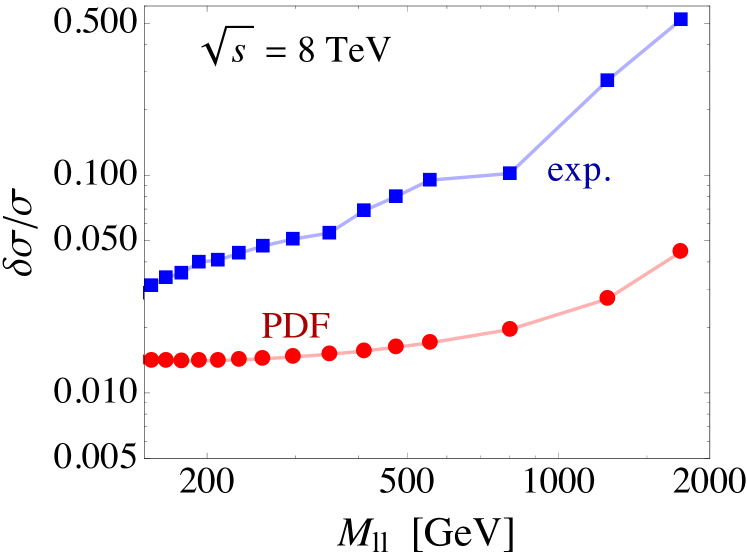
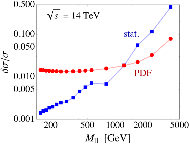
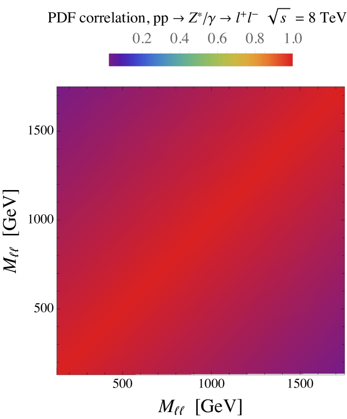
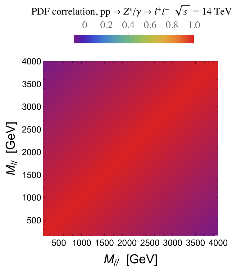
Figure 3: Impact of PDF uncertainties. Upper row, left panel. Comparison between the experimental error (blue) and the PDF uncertainty (red) at $\sqrt{s}=8$ TeV. The experimental errors take into account both statistical error and systematic uncertainties, as described in CMS:2014jea . Upper row, right panel. Comparison between the statistical error (blue) and the PDF uncertainty (red) at $\sqrt{s}=14$ TeV. Lower row. Correlation matrix at $\sqrt{s}=8$ TeV (left) and $\sqrt{s}=14$ TeV (right).

We show our results in the left column of Fig. 3. In the upper plot, we show the relative PDF errors per individual bin (red circles), and we compare them with the experimental errors quoted in CMS:2014jea ; hepdata_DY (blue squares). As clear from this plot, at $\sqrt{s}=8$ TeV the impact of PDF uncertainties is sub-leading if compared with the experimental errors. For completeness, in the lower panel we show the PDF correlation extracted according to Eq. (23).

Let us now discuss our findings, shown in the left panel of Fig. 4 where we plot the $1$-, $2$- and $3\,\sigma$ bound. First of all, it is interesting to compare the DY bound with the constraint placed by LEP in Fig. 1. The net result is that the measurement of the DY differential cross-section at large invariant mass at the LHC with $\sqrt{s}=8$ TeV already provides a bound stronger than the one obtained at LEP. This is a conceptually remarkable result, given the penalizing price unavoidably paid by an hadronic machine like the LHC in performing precision measurements. Notwithstanding this important observation, it is also clear from Fig. 4 that the DY bound extracted at $\sqrt{s}=8$ TeV does not rule out any relevant portion of the parameter space since it requires at least $d_{X}N_{X}Q_{X}^{2}\gtrsim 50$, a value objectively too large for any realistic model.

However, encouraged by the promising result obtained at $\sqrt{s}=8$ TeV, we move now to explore future prospects at $\sqrt{s}=14$ TeV.

4.2 Drell-Yan at $\sqrt{s}=14$ TeV

At $\sqrt{s}=14$ TeV we have to rely on a projection. We generate mock data assuming that the observed invariant mass distribution agrees with the NNLO QCD SM prediction. We include the effect of running couplings according to Eq. (19), and we construct a $\chi^{2}$ distribution as in Eq. (20)—thus including an overall free normalization $\mathcal{N}$ as nuisance parameter to account for correlated unknown systematic uncertainties. We write the covariance error matrix as

$$\Sigma=\Sigma_{\rm stat}+\Sigma_{\rm uncorr\,syst}+\Sigma_{\rm PDF}~{}.$$ (25)

Statistical errors are obtained assuming an integrated luminosity $\mathcal{L}=300$ fb^-1, and converting the cross-section in terms of number of events per bin. The corresponding covariance error matrix $\Sigma_{\rm stat}$ is diagonal, with entries equal to the square of the statistical errors. The PDF uncertainties are estimated as discussed before (see Eqs. (22,23)). We show our results in the right column of Fig. 3. Finally, $\Sigma_{\rm uncorr\,syst}$ is built assuming a flat $1\%$ ($2.5\%$) uncertainty across all invariant mass bins in order to simulate the presence of uncorrelated systematic errors.

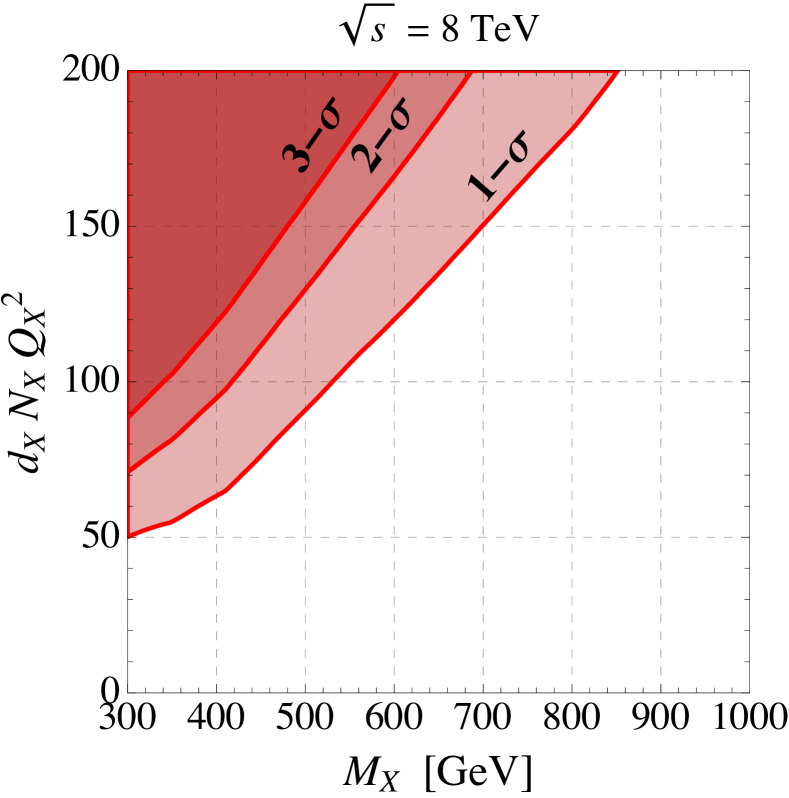
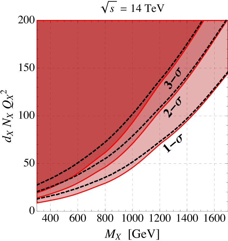
Figure 4: Left panel. $1$-, $2$- and $3$-$\sigma$ bound at $\sqrt{s}=8$ TeV. Right panel. $1$-, $2$- and $3$-$\sigma$ bound at $\sqrt{s}=14$ TeV. Solid red (dashed black) lines were obtained including $1\%$ ($2.5\%$) uncorrelated systematic error.

At $\sqrt{s}=14$ TeV the simulated data extend up to $M_{ll}\simeq 5$ TeV; the statistical error, assuming $\mathcal{L}=300$ fb^-1, does not exceed the $10\%$ level up to $M_{ll}\simeq 2$ TeV as shown in the upper-right panel of Fig. 3. At invariant mass $M_{ll}\lesssim 1$ TeV the statistical error stays below $1\%$, and the PDF error, as well as the uncorrelated systematic error, starts to become important. From this simple estimate it is clear that the constraining power of the DY differential cross-section at $\sqrt{s}=14$ TeV will lead to much stronger bounds w.r.t. those obtained in section 4.1 using data at $\sqrt{s}=8$ TeV.

We show our findings in the right panel of Fig. 4 where we plot the $1$-, $2$- and $3\,\sigma$ bound. The solid (dashed) contours in red (black) were obtained considering $1\%$ ($2.5\%$) uncorrelated systematic uncertainties. The impact of these uncorrelated systematic uncertainties is particularly important for light vector-like fermions and small values of $d_{X}N_{X}Q_{X}^{2}$, where the deviation due to running couplings is smaller and thus it can be more easily hidden in the uncertainty accompanying the measured cross-section. Despite this, it is clear that the constraining power (or, said differently, the discovery potential) of the DY process at the LHC with $\sqrt{s}=14$ TeV and $300$ fb^-1 starts to bite into an interesting region of the parameter space where, in particular for light vector-like fermions, the effective coupling $d_{X}N_{X}Q_{X}^{2}$ is lowered down to phenomenologically realistic values. In section 5 we will discuss the implication of the DY process for the diphoton excess at $750$ GeV.

It is possible to speculate even further about the role of the DY process as precision observable at the LHC. As clear from the upper right panel of Fig. 3, the dominant error at large dilepton invariant mass comes from limited statistics. The High Luminosity LHC (HL-LHC) program has the scope of attaining the threshold of $3000$ fb^-1 of integrated luminosity. In this case, reducing the statistical error by roughly a factor $10$, it would be possible to largely improve the constraining power/discovery potential of the DY channel even for vector-like states with TeV-scale mass.

4.3 New charged scalars

Before proceeding, let us briefly discuss the case in which the SM is extended by adding $N_{X}$ complex singlet scalars $X$ with mass $M_{X}$ and hypercharge $Y=Q_{X}$. For a more general discussion we refer the reader to Salvio:2016hnf . At one loop, the contributions to the $\mathcal{Y}$ parameter and the hypercharge one-loop $\beta$ function are

$$\mathcal{Y}=d_{X}N_{X}Q_{X}^{2}\,\frac{\alpha_{Y}m_{W}^{2}}{120\pi M_{X}^{2}}~{},~{}~{}~{}~{}\beta_{g_{1}}^{(1)}=\left(\frac{41}{10}+d_{X}N_{X}Q_{X}^{2}\frac{1}{5}\right)g_{1}^{3}~{},$$ (26)

where, in parallel with the fermionic case, the number of effective degrees of freedom $d_{X}N_{X}$ accounts for possible color multiplicity. If compared to the fermionic case, the scalar contribution to the $\mathcal{Y}$ parameter turns out to be eight times smaller, and the bound from LEP becomes irrelevant even for very light scalar particles. In the absence of any constraint from LEP, it is important to assess the constraining power of the DY analysis at the LHC. Using the fermionic case as basis for comparison, from Eq. (26) we see that the impact of a charged scalar particle on the $g_{1}$ running is four times smaller. We therefore expect a weaker bound from the DY analysis. To fix ideas, at $\sqrt{s}=8$ TeV and for $M_{X}=400$ GeV we find that the running induced by new charged scalar particles produces a $10\%$ correction to the differential cross-section at $M_{ll}=800$ GeV only for $d_{X}N_{X}Q_{X}^{2}\simeq 270$. Contrarily, at $\sqrt{s}=14$ TeV and for $M_{X}=400$ GeV a $2\%$ deviation at $M_{ll}=1000$ GeV can be obtained with $d_{X}N_{X}Q_{X}^{2}\simeq 50$. We therefore conclude that the constraining power of the DY process in the scalar case is only marginally relevant even considering collisions at $\sqrt{s}=14$ TeV with large integrated luminosity.

4.4 FCC-ee

The FCC-ee is a high-luminosity, high-precision $e^{+}e^{-}$ circular collider envisioned in a new $80-100$ km tunnel in the Geneva area with a centre-of-mass energy from $90$ to $400$ GeV TLEP. Thanks to its clean experimental environment, the FCC-ee collider could explore the EW physics with unprecedented accuracy, allowing for a careful scrutiny of new physics models predicting new particles at the TeV scale and beyond. In the following, we base our discussion on Gomez-Ceballos:2013zzn .

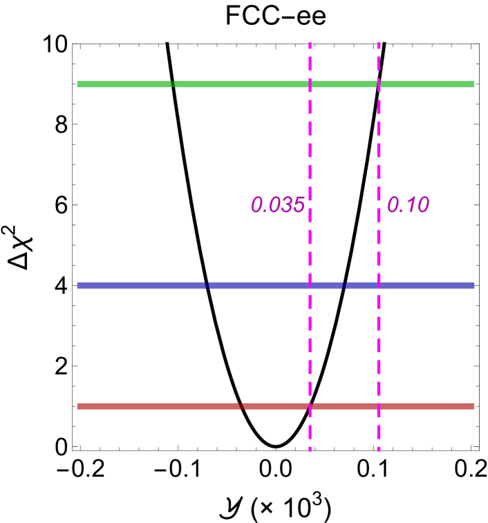
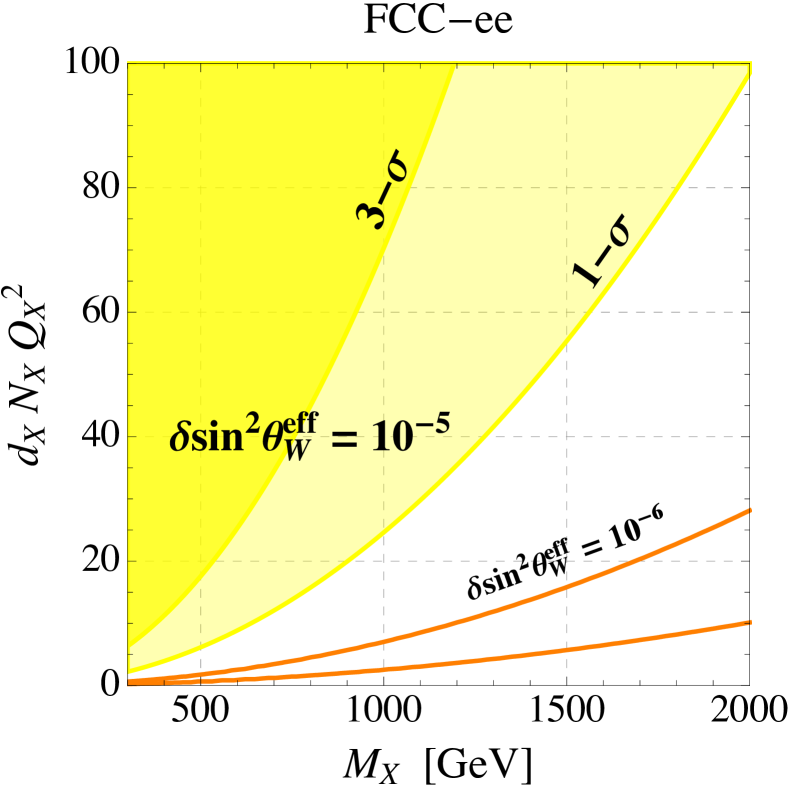
Figure 5: Left panel. One-parameter fit of LEP data in terms of the $\mathcal{Y}$ parameter. We rescale the errors of the EW precision measurements according to what expected in Gomez-Ceballos:2013zzn for a future circular $e^{+}e^{-}$ collider in order to provide a flavor of its constraining power (see text for details). We set the precision on the effective squared mixing angle to $\delta\sin^{2}\theta_{W}^{\rm eff}=10^{-5}$. The central value of $\mathcal{Y}$ is arbitrarily set to zero. Right panel. $1$- and $3$-sigma exclusion regions in terms of the parameter space $(d_{X}N_{X}Q_{X}^{2},M_{X})$ (yellow). We also show the corresponding bounds if $\delta\sin^{2}\theta_{W}^{\rm eff}=10^{-6}$ (orange).

To give an idea of the constraining power of the FCC-ee collider, it is possible to recast the LEP results. For instance, according to the estimates presented in Gomez-Ceballos:2013zzn , at the FCC-ee it will be possible to measure the pole mass of the Z-boson with a precision twenty times smaller than the one reached at LEP, $\left.\delta m_{Z}\right|_{\rm LEP}=0.0021$ GeV. One can fit the LEP data implementing all the upgraded precisions quoted in Gomez-Ceballos:2013zzn . Following this logic, we show in the left panel of Fig. 5 the bound obtained considering a one-parameter fit made in terms of the $\mathcal{Y}$ parameter. The most important measurement controlling the precision on $\mathcal{Y}$ is the square of the effective weak mixing angle. Assuming $\delta\sin^{2}\theta_{W}^{\rm eff}=10^{-5}$, we find $\delta\mathcal{Y}=0.035\times 10^{-3}\,(0.1\times 10^{-3})$ at $1$-$\sigma$ ($3$-$\sigma$). In the right panel of Fig. 5 we translate these confidence regions in the parameter space $(d_{X}N_{X}Q_{X}^{2},M_{X})$ (regions shaded in yellow). As expected the constraining power of the FCC-ee collider turns out to be much stronger than the capabilities of present and future LHC searches in the DY channel. If $\delta\sin^{2}\theta_{W}^{\rm eff}=10^{-6}$ (the value envisaged in Gomez-Ceballos:2013zzn ) the constraint becomes even stronger, and we find $\delta\mathcal{Y}=0.0036\times 10^{-3}\,(0.01\times 10^{-3})$ (orange lines in the right panel of Fig. 5).

5 Implications for the Diphoton Excess at $750$ GeV

We are now in the position to comment about the importance of the DY process at the LHC for the diphoton excess discussed in section 2. The Yukawa interactions between the (pseudo-) scalar resonance $S$ and the vector-like fermions $X$ are encoded in the Lagrangian

$$\mathcal{L}=\mathcal{L}_{SM}+\frac{(\partial_{\mu}S)^{2}}{2}+\bar{X}(i\not{D}-M_{X})X-\left[S\bar{X}(y_{X}+i\tilde{y}_{X}\gamma^{5})X+h.c.\right]-V(S)-V(S,H)~{},$$ (27)

where $\mathcal{L}_{SM}$ is the SM Lagrangian and where we assumed that the $N_{X}$ fermions have the same mass and couplings. The Yukawa coupling $y$ ($\tilde{y}$) is present if $S$ is a scalar (pseudo-scalar). The potential is $V(S)=(M_{S}^{2}/2)S^{2}+\lambda_{S}S^{4}$, and $V(S,H)$ accounts for possible interactions with the Higgs doublet $H$. The explicit form of $V(S,H)$ is not important for the purposes of our discussion, and we refer to Salvio:2016hnf for a more general analysis including vacuum stability.

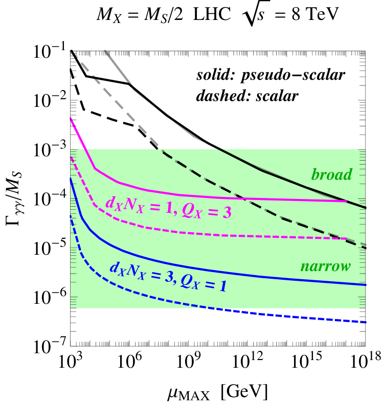
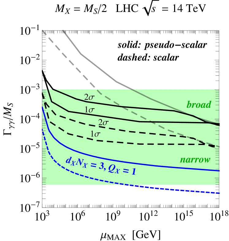
Figure 6: Maximal diphoton decay width for a pseudo-scalar (solid lines) and scalar (dashed lines) resonance as a function of the scale at which the theory becomes non-perturbative. The gray lines include the LEP bound on the $\mathcal{Y}$ parameter at $1$-$\sigma$ level. The black lines include the LHC bound from DY at $\sqrt{s}=8$ TeV ($1$-$\sigma$ contour, left panel) $\sqrt{s}=14$ TeV ($1$- and $2$-$\sigma$ contours, right panel). We also show two particular cases with $d_{X}N_{X}=3$, $Q_{X}=1$ (blue), $d_{X}N_{X}=1$, $Q_{X}=3$ (magenta).

As pointed out in Gu:2015lxj ; Goertz:2015nkp ; Son:2015vfl , it is important to keep track of the RG evolution of the Yukawa coupling since it can easily exceed the perturbative regime. The Yukawa couplings $y_{X}$ and $\tilde{y}_{X}$ have the same RGE, and we find

$$\beta_{y_{X}}^{(1)}=\left[\left(2d_{X}N_{X}+3\right)y_{X}^{2}-\frac{18}{5}Q_{X}^{2}g_{1}^{2}\right]y_{X}~{}.$$ (28)

The CP-odd coupling $\tilde{y}_{X}$ contributes to the diphoton decay width of $S$ more than the CP-even coupling $y_{X}$. For the latter, we have

$$\frac{\Gamma_{\gamma\gamma}}{M_{S}}=\frac{\alpha^{2}}{16\pi^{3}}\left|d_{X}N_{X}Q_{X}^{2}y_{X}\sqrt{\tau_{X}}\mathcal{S}(\tau_{X})\right|^{2}~{},$$ (29)

with $\tau_{X}\equiv 4M_{X}^{2}/M_{S}^{2}$. The pseudo-scalar case corresponds to the substitutions $y_{X}\to\tilde{y}_{X}$, $\mathcal{S}(\tau_{X})\to\mathcal{P}(\tau_{X})$.

In Fig. 6 we show the maximal diphoton decay width of the (pseudo-) scalar resonance $S$ as a function of the scale at which the theory becomes non-perturbative. In more detail, our logic goes as follows. i) For a given value of $d_{X}N_{X}$, $Q_{X}$ and $y_{X}$ ($\tilde{y}_{X}$) we compute the scale at which the theory becomes non-perturbative by solving the RGEs for $g_{1}$ and $y_{X}$ ($\tilde{y}_{X}$). The x-axes in Fig. 6 is therefore formally defined as the scale $\mu_{\rm max}$ at which either $y_{X}(\tilde{y}_{X})=4\pi$ (perturbativity of the Yukawa coupling) or $g_{1}=\infty$ (hypercharge Landau pole) is realized along the RG flow. ii) By scanning over $d_{X}N_{X}$, $Q_{X}$ and $y_{X}$ ($\tilde{y}_{X}$), and using Eq. (29), we can compute the maximal diphoton decay width that the (pseudo-) scalar resonance $S$ can obtain for a given $\mu_{\rm max}$. To give an even more clear understanding, we also show in Fig. 6 the maximal $\Gamma_{\gamma\gamma}$ corresponding to fixed values of $d_{X}N_{X}$, $Q_{X}$. For a fixed value of $d_{X}N_{X}$, $Q_{X}$ one has the freedom to move on the corresponding line by changing the Yukawa coupling. Large Yukawa couplings correspond to the left-most part of the plot, where the diphoton width $\Gamma_{\gamma\gamma}$ rapidly increases (being proportional to $y_{X}^{2}$ ($\tilde{y}_{X}^{2}$)) at the prize to lower the cut-off scale of the theory down to the TeV range. iii) Finally, we impose—at each point $d_{X}N_{X}$, $Q_{X}$—the LEP and LHC constraint derived in section 2 and section 4. In the left (right) panel of Fig. 6 we include the impact of the $1$- and $2$-$\sigma$ bounds derived from the analysis at $\sqrt{s}=8$ TeV ($\sqrt{s}=14$ TeV): Every point in the scan violating such bound is discarded.

Following the logic explained above, in Fig. 6 we show the maximal diphoton decay width for a scalar (dashed lines) and pseudo-scalar (solid lines) resonance $S$ as a function of the cut-off scale $\mu_{\rm max}$. For simplicity, we fix $M_{X}=M_{S}/2$ since this value maximizes the diphoton width. Gray lines include only the bound from LEP, while the black lines include the bound extracted by the DY analysis at the LHC. The cases with $d_{X}N_{X}=3$, $Q_{X}=1$ and $d_{X}N_{X}=1$, $Q_{X}=3$ are shown in blue and magenta. We are interested in values $10^{-6}\lesssim\Gamma_{\gamma\gamma}/M_{S}\lesssim 10^{-3}$, where the left (right) part of the disequality corresponds to narrow (large) width, as discussed in section 2. In this respect, the bound from LEP plays non role in constraining phenomenologically interesting values of $\Gamma_{\gamma\gamma}/M_{S}$. At $\sqrt{s}=8$ TeV, the DY bound bites into a small corner of the parameter space, as clear from the comparison between the gray and the black lines in the left panel of Fig. 6. However, it does not have any relevant implications w.r.t. the diphoton excess. At $\sqrt{s}=14$ TeV, the story changes. The DY bound starts to become relevant. In the scalar case the black line is lowered down to $\Gamma_{\gamma\gamma}/M_{S}\simeq 10^{-4}-10^{-5}$ (at, respectively, $2$- and $1$-$\sigma$), thus affecting the whole region of the parameter space favored by the large width assumption. The pseudo-scalar case gives a similar result, with the maximal diphoton width lowered down to $\Gamma_{\gamma\gamma}/M_{S}\simeq 10^{-3}-10^{-4}$.

To conclude, we argue that the new physics involved in the explanation of the diphoton excess at $750$ GeV could leave—especially if the indications in favor of a large width will be confirmed—a footprint in the differential cross-section of the neutral DY process at large dilepton invariant mass.

6 Comments on direct searches for the new states

In this section let us shortly comment on the direct detection of the new states. Of course, direct detection reach strongly depends on the particular decay modes of the vector like fermions. Comparing these searches to the indirect searches via DY production is by no mean straightforward. Surveying all various possibilities in terms of hypercharge and decay chains is well beyond the scope of this paper. Therefore, we will just emphasize several points, which are generic to the EW production. By drawing analogy to the existing searches for the EW pair-produced states we will merely try to give a flavor of what might the ballpark of the direct detection bounds.

At the partonic level, the cross section for the on-shell production of a $X\bar{X}$ pair is

$$\sigma_{q\bar{q}}(\hat{s})=\frac{\pi\alpha^{2}Q_{X}^{2}}{162c_{W}^{2}(s-M_{Z}^{2})^{2}}\sqrt{1-\frac{4M_{X}^{2}}{\hat{s}}}s\left(1+\frac{2M_{X}^{2}}{s}\right)\mathcal{P}_{q\bar{q}}\left(\frac{M_{Z}^{2}}{s}\right)~{},$$ (30)

where

$$\mathcal{P}_{u\bar{u}}(x) \equiv 17-40c_{W}^{2}x+32c_{W}^{4}x^{2}~{},$$ (31)

$$\mathcal{P}_{d\bar{d}}(x) \equiv 5-4c_{W}^{2}x+8c_{W}^{4}x^{2}~{},$$ (32)

for, respectively, up- and down-type quarks in the initial partonic state. The cross-section $pp\to X\bar{X}$ for producing a vector-like fermion pair with charge $Q_{X}$ at the LHC with $\sqrt{s}=8,\,14$ TeV is shown in Fig. 7.

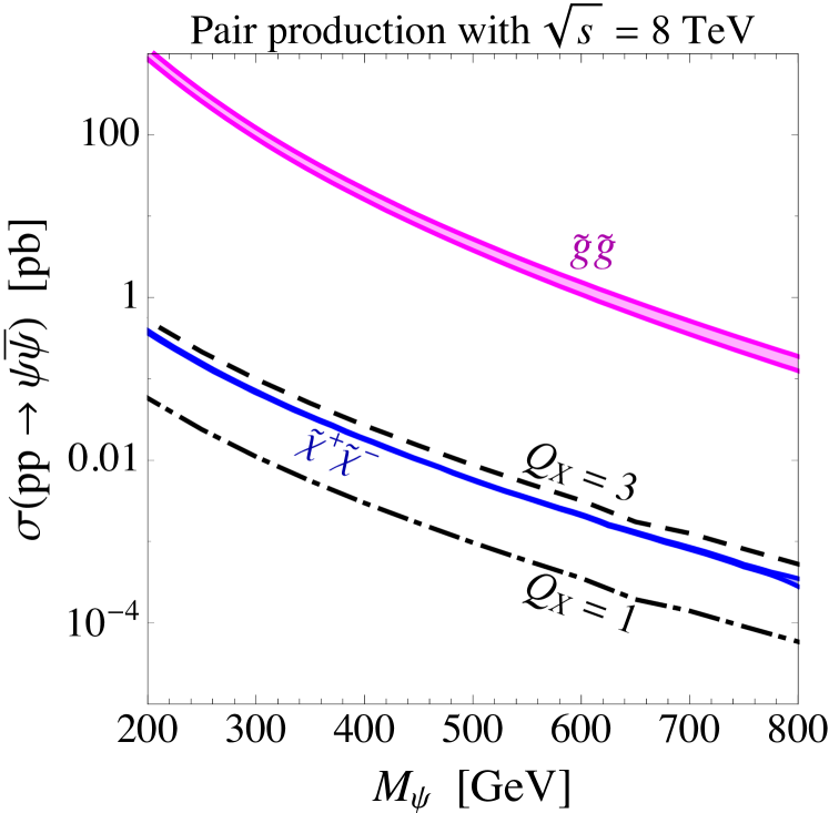
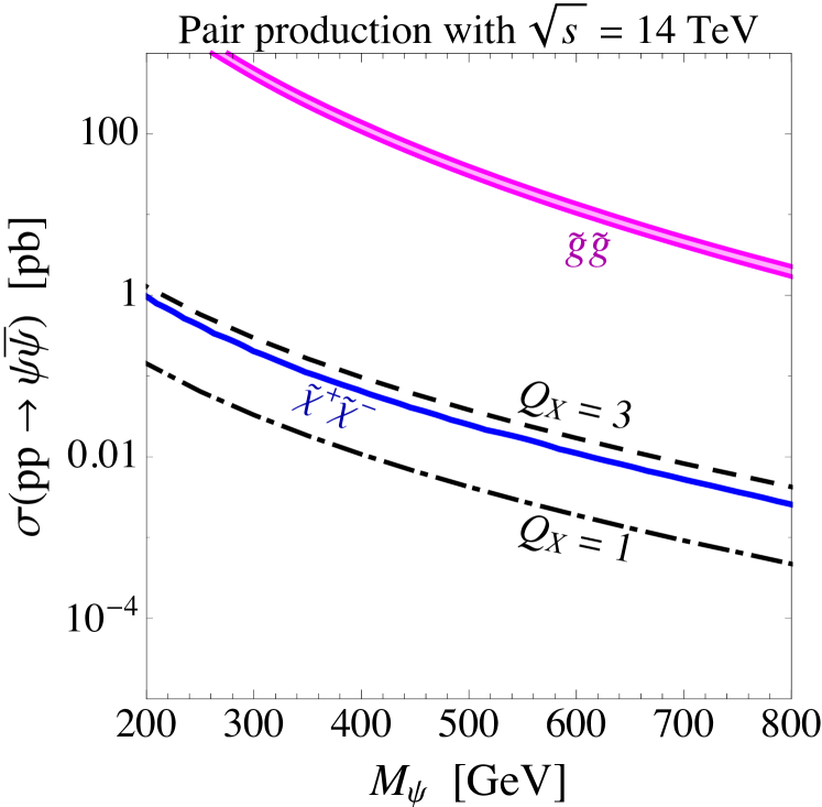
Figure 7: Cross-section $pp\to X\bar{X}$ for producing two fermions with charge $Q_{X}$ at $\sqrt{s}=8$ TeV (left panel) and $\sqrt{s}=14$ TeV (right panel). The blue (magenta) line stands for the production cross sections of wino charginos (gluinos) in SUSY.

Naively one would expect that the production cross sections are EW, not that different, for example, from SUSY EW-ino production cross sections. In general it is right, however the cross sections that we get for a single state are generally smaller than typical EW cross sections. The pair-production cross section of a single, charge-one state, is smaller than the production cross sections of the SUSY charged winos (cf. Fig. 7). The explanation is very simple: our production is proportional to the $\alpha_{Y}^{2}$ rather than $\alpha_{2}^{2}$ which suppresses the cross sections by more than order of magnitude. On the other hand, if all the new states lie at the same mass scale, we expect the total cross sections to be increased by factor of $d_{X}N_{X}Q_{X}^{2}$. Therefore, when both these factors are taken into account we end up with the cross sections, which are slightly bigger (by order-one factor) than the standard EW cross sections.

Most of the searches for the EW states at the LHC for now, are motivated by the SUSY EW-ino. This usually ends up in final states leptons (including, possibly, taus) and with $\not{E}_{T}$. Although we do not know, what would be exactly the bounds on every single scenario one would consider, the direct detection bounds are very unlikely to exceed the bounds on the SUSY wino-chargino particles. The bound on chargino is around 475 GeV if it is assumed to decay to the electrons or muons Aad:2014vma , and it is around 360 GeV if we are considering decays into taus Aad:2014yka .

7 Conclusions

In this paper we made one of the first attempts to confront some theoretical explanations of the diphoton access with LHC SM precision measurements. Phenomenological models which try to fit the large width of diphoton excess, suggested by ATLAS, suggest large multiplicity of the EW-charged states below the TeV scale that have a significant impact on the hypercharge coupling running. We point out that this running can be probed via DY production at the LHC, estimate the bounds from LHC8 and project the bounds from the LHC14. We show, that contrary to the direct detection our method is robust and it can clearly exclude or confirm such new states at the EW scale.

Interestingly the bounds that we derive from the LHC8, although still relatively weak, are already much stronger that the bounds one get from LEP. Moreover, LHC14 DY measurements will significantly improve the reach, pushing the bounds (or maybe making discoveries) deep into the parameter space relevant for the wide 750 GeV resonance.

We also briefly comment on the possibilities of the direct detection of the new EW states at the LHC. Unfortunately this question is much more model dependent, and lacks the robustness of the precision measurement approach. While it is relatively easy to hide the new states from the direct detection by assuming complicated decay chains and large multiplicity state, it would be interesting to survey more carefully various decay modes.

Appendix A Simulating the theoretical prediction for the DY at the LHC

We describe the theory framework used to derive the predictions for the DY cross section $d\sigma_{\rm DY}/dm\equiv d\sigma(pp\to Z,\gamma\to\ell^{+}\ell^{-})/dm_{\ell^{+}\ell^{-}},\ \ell=e\text{ or }\mu$, at the LHC, binned in $m_{\ell^{+}\ell^{-}}$ as described in hepdata_DY . We employ the code FEWZ Gavin:2010az , version 3.1b2, which includes NNLO QCD and NLO EW corrections to the process. The cross section is considered over the full phase space, i.e., no cuts are applied - beyond the standard $p_{T}>10\,$GeV ($p_{T}>20\,$GeV, $\eta<4.5$) cuts on real photons (jets). We use CTEQ12NNLO pdfs and chose a dynamical scale of $\mu_{R}=\mu_{F}=m_{\ell^{+}\ell^{-}}$.

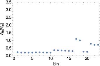
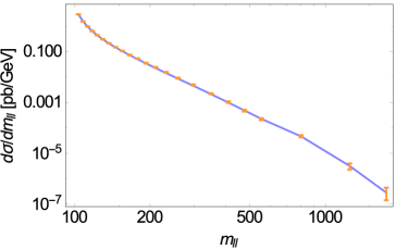
Figure 8: Left: Monte Carlo error quoted by FEWZ for each bin in per mille. Right: Theoretical prediction for the cross section $d\sigma_{\rm DY}/dm$ (blue line), overlayed with the corresponding experimental results (orange error bars), at $\sqrt{s}=8\,$ TeV. See text for details.

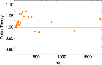
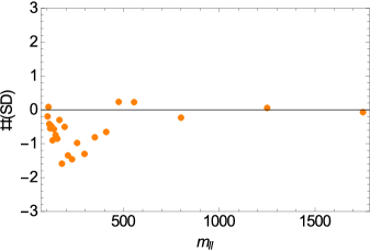
Figure 9: Left: Ratio $\sigma_{\rm DY}^{\rm th}/\sigma_{\rm DY}^{\rm exp}$. Right: Difference between theory prediction and experimental results in standard deviations. See text for details.

As CMS presents their data hepdata_DY after unfolding actually both initial state and final state radiation (employing Monte Carlo simulation), we set EW control = 7 in FEWZ. This removes the main source of difference between final state electrons and muons.

Moreover, we turn off the photon-induced channel via setting Alpha QED(0)=0, since it has been removed in the results as given in hepdata_DY ; CMS:2014jea . The other physical parameters are kept as in the FEWZ default, in particular we employ the $G_{\mu}$ input scheme and use the $Z-$pole focus.

$m_{\ell^{+}\ell^{-}}$ [GeV]	$d\sigma_{\rm DY}/dm$ [pb/GeV]	$\delta_{\rm th}$ [pb/GeV]
103.5	2.95064	0.000695558
108	1.55449	0.00032792
112.5	0.975046	0.000205666
117.5	0.641322	0.000133134
123	0.440523	0.0000928767
129.5	0.303344	0.0000691137
137	0.210305	0.0000469974
145.5	0.1469	0.0000319788
155	0.103285	0.0000220165
165.5	0.0730464	0.000015263
178	0.0505791	0.0000186166
192.5	0.0343989	0.0000123249
210	0.0227222	$7.9255\times 10^{-6}$
231.5	0.0143423	$4.81843\times 10^{-6}$
258	0.0086692	$2.78966\times 10^{-6}$
296.5	0.00458432	$1.41792\times 10^{-6}$
350	0.00211278	$2.3279\times 10^{-6}$
410	0.000987678	$9.93302\times 10^{-7}$
475	0.000484899	$1.31907\times 10^{-7}$
555	0.000225813	$5.88447\times 10^{-8}$
800	0.0000459948	$3.62253\times 10^{-8}$
1250	$3.13852\times 10^{-6}$	$2.24954\times 10^{-9}$
1750	$2.79568\times 10^{-7}$	$2.01314\times 10^{-10}$

Table 1: Theory prediction for the DY cross section at $\sqrt{s}=8\,$ TeV together with the Monte Carlo error. The central values of the bins in $m_{\ell^{+}\ell^{-}}$ are quoted in the first column. See text for details.

It turns out that the accuracy of the results in the large $m_{\ell^{+}\ell^{-}}$ bins could be improved by running each bin individually - allowing to generate sufficient Monte Carlo statistic also for high-mass bins (which have a limited impact on the total cross section). We show the resulting errors quoted by FEWZ (not including pdf uncertainties or scale variation) for $\sqrt{s}=8\,$ TeV in the left panel of Figure 8 – demonstrating that the Monte Carlo error seems under good control in all bins, i.e.,

$$\delta_{\rm th}\equiv\delta\sigma_{\rm DY}^{\rm th}/\sigma_{\rm DY}^{\rm th}\lesssim 1\permil~{}.$$ (33)

Finally, we present our $\sqrt{s}=8\,$ TeV results for the differential cross section in Table 1, including the FEWZ errors. We also provide in the right panel of Figure 8 a simultaneous plot of our predictions (blue, joined - neglecting the small $\delta_{\rm th}$) and the experimental results as given in hepdata_DY (orange - including the quoted error bars). Moreover, in the left and right panels of Figure 9, we present for completeness the ratio $\sigma_{\rm DY}^{\rm th}/\sigma_{\rm DY}^{\rm exp}$ and the difference between theory and experiment in standard deviations, adding the corresponding errors in quadrature.

References

- (1) ATLAS Collaboration, Search for resonances decaying to photon pairs in 3.2 fb-1 of collisions at = 13 TeV with the ATLAS detector, .
- (2) CMS Collaboration, Search for new physics in high mass diphoton events in proton-proton collisions at 13TeV, .
- (3) R. Franceschini, G. F. Giudice, J. F. Kamenik, M. McCullough, A. Pomarol, R. Rattazzi, M. Redi, F. Riva, A. Strumia, and R. Torre, What is the gamma gamma resonance at 750 GeV?, arXiv:1512.04933.
- (4) S. Knapen, T. Melia, M. Papucci, and K. Zurek, Rays of light from the LHC, arXiv:1512.04928.
- (5) J. Ellis, S. A. R. Ellis, J. Quevillon, V. Sanz, and T. You, On the Interpretation of a Possible GeV Particle Decaying into , arXiv:1512.05327.
- (6) S. D. McDermott, P. Meade, and H. Ramani, Singlet Scalar Resonances and the Diphoton Excess, arXiv:1512.05326.
- (7) A. Angelescu, A. Djouadi, and G. Moreau, Scenarii for interpretations of the LHC diphoton excess: two Higgs doublets and vector-like quarks and leptons, arXiv:1512.04921.
- (8) R. S. Gupta, S. Jäger, Y. Kats, G. Perez, and E. Stamou, Interpreting a 750 GeV Diphoton Resonance, arXiv:1512.05332.
- (9) M. Bauer and M. Neubert, Flavor Anomalies, the Diphoton Excess and a Dark Matter Candidate, arXiv:1512.06828.
- (10) A. Salvio, F. Staub, A. Strumia, and A. Urbano, On the maximal diphoton width, arXiv:1602.01460.
- (11) J. Gu and Z. Liu, Running after Diphoton, arXiv:1512.07624.
- (12) F. Goertz, J. F. Kamenik, A. Katz, and M. Nardecchia, Indirect Constraints on the Scalar Di-Photon Resonance at the LHC, arXiv:1512.08500.
- (13) M. Son and A. Urbano, A new scalar resonance at 750 GeV: Towards a proof of concept in favor of strongly interacting theories, arXiv:1512.08307.
- (14) D. S. M. Alves, J. Galloway, J. T. Ruderman, and J. R. Walsh, Running Electroweak Couplings as a Probe of New Physics, JHEP 02 (2015) 007, [arXiv:1410.6810].
- (15) M. R. Buckley, Wide or Narrow? The Phenomenology of 750 GeV Diphotons, arXiv:1601.04751.
- (16) A. Falkowski, O. Slone, and T. Volansky, Phenomenology of a 750 GeV Singlet, arXiv:1512.05777.
- (17) R. Barbieri, A. Pomarol, R. Rattazzi, and A. Strumia, Electroweak symmetry breaking after LEP-1 and LEP-2, Nucl. Phys. B703 (2004) 127–146, [hep-ph/0405040].
- (18) A. D. Martin, W. J. Stirling, R. S. Thorne, and G. Watt, Parton distributions for the LHC, Eur. Phys. J. C63 (2009) 189–285, [arXiv:0901.0002].
- (19) CMS Collaboration, V. Khachatryan et al., Measurements of differential and double-differential Drell-Yan cross sections in proton-proton collisions at 8 TeV, Eur. Phys. J. C75 (2015), no. 4 147, [arXiv:1412.1115].
- (20) “The Durham HepData Project: Measurements of differential and double-differential Drell-Yan cross sections in proton-proton collisions at 8 TeV.” http://hepdata.cedar.ac.uk/view/ins1332509.
- (21) R. Gavin, Y. Li, F. Petriello, and S. Quackenbush, FEWZ 2.0: A code for hadronic Z production at next-to-next-to-leading order, Comput. Phys. Commun. 182 (2011) 2388–2403, [arXiv:1011.3540].
- (22) A. Buckley, J. Ferrando, S. Lloyd, K. Nordstr m, B. Page, M. R fenacht, M. Sch nherr, and G. Watt, LHAPDF6: parton density access in the LHC precision era, Eur. Phys. J. C75 (2015) 132, [arXiv:1412.7420].
- (23) TLEP Design Study Working Group Collaboration, M. Bicer et al., First Look at the Physics Case of TLEP, JHEP 01 (2014) 164, [arXiv:1308.6176].
- (24) ATLAS Collaboration, G. Aad et al., Search for direct production of charginos, neutralinos and sleptons in final states with two leptons and missing transverse momentum in collisions at 8 TeV with the ATLAS detector, JHEP 05 (2014) 071, [arXiv:1403.5294].
- (25) ATLAS Collaboration, G. Aad et al., Search for the direct production of charginos, neutralinos and staus in final states with at least two hadronically decaying taus and missing transverse momentum in collisions at = 8 TeV with the ATLAS detector, JHEP 10 (2014) 096, [arXiv:1407.0350].
- (26) C. Gross, O. Lebedev, and J. M. No, Drell-Yan Constraints on New Electroweak States and the Di-photon Anomaly, arXiv:1602.03877.