Integrative Dynamic Reconfiguration in a
Parallel Stream Processing Engine

Abstract

Load balancing, operator instance collocations and horizontal scaling are critical issues in Parallel Stream Processing Engines to achieve low data processing latency, optimized cluster utilization and minimized communication cost respectively. In previous work, these issues are typically tackled separately and independently. We argue that these problems are tightly coupled in the sense that they all need to determine the allocations of workloads and migrate computational states at runtime. Optimizing them independently would result in suboptimal solutions. Therefore, in this paper, we investigate how these three issues can be modeled as one integrated optimization problem. In particular, we first consider jobs where workload allocations have little effect on the communication cost, and model the problem of load balance as a Mixed-Integer Linear Program. Afterwards, we present an extended solution called ALBIC, which support general jobs. We implement the proposed techniques on top of Apache Storm, an open-source Parallel Stream Processing Engine. The extensive experimental results over both synthetic and real datasets show that our techniques clearly outperform existing approaches.

1 Introduction

Recently, Parallel Stream Processing Engines (PSPEs) are emerging to process the ever growing big streams of data generated by mobile devices, sensors, online social networks, online financial transactions, and so on. Representatives of modern PSPEs include Apache Storm [38], Apache S4 [30] and Google MillWheel [7]. A job in an PSPE consists of a set of operators, and each operator is usually parallelized into a number of instances, each processing a subset of the operator’s input to increase the data throughput. The output of the instances of upstream operators, except the sink operators, is input to their downstream neighbors, forming a pipelined network, called the topology of the job.

In general, there are three highly correlated job optimization problems in a PSPE. First of all, load balancing across the processing nodes is critical to maximizing cluster utilization and minimizing data processing latency especially during temporary load spikes. While load balancing in parallel computing systems [31, 34] has been studied extensively in the literature, developing load balancing mechanisms in PSPEs faces new challenges. Operator instances in PSPEs are long-standing, and probably need to be reallocated many times during their life-time. In other words, load rebalancing decisions have to be made continuously and periodically to maintain satisfactory system performance. As operator instances in PSPEs may be associated with computing states and their reallocations may involve state migrations with significant overheads, load balancing decisions have to take such overheads into account.

Secondly, neighboring operator instances in PSPEs continuously transfer data between each other. Collocating them at the same node will significantly reduce the system’s workload by eliminating the overhead of cross-node data transmission, which includes both network bandwidth consumption [32, 6] and CPU consumption caused by data serialization and deserialization. Moreover, the fact that the load of an operator instance is correlated with its relative location to its neighbors also complicates the problem of load balancing. Assigning a location-independent load value to each instance cannot model the real situation and hence cannot optimize the performance. To simplify the problem, previous studies of dynamic load balancing in PSPEs, such as [36, 41, 45, 29] largely ignore the effect of collocating operator instances.

Thirdly, with the development of cloud computing platforms and distributed system kernels (such as Mesos [16]), horizontal scaling of an PSPE, i.e. the ability to dynamically acquire and relinquish computing resources at runtime, is crucial to achieve high resource utilization and low operational cost. We argue that the problem of horizontal scaling is tightly coupled with both load balancing and operator instance collocation. For example, the overload of the system could possibly be rectified by collocating operator instances that have a high communication volume between each other to save the cost of data serialization and deserialization instead of acquiring more resources. Another example is that horizontal scaling, load balancing and operator instance collocation all involve state migrations, which may incur significant overhead. Hence optimizing them integratively would result in a solution with better load balancing and lower overhead. However, there is a lack of study on how to perform such an integrative optimization.

To fill the gap, we revisit the load balancing problem in PSPEs and propose a novel solution that also takes operator instance collocation and horizontal scaling into account. We first study the scenarios where collocating operator instances has little effect. Such scenarios occur when each operator instance has to transfer data to a lot of neighbors evenly. We model this problem as a Mixed-Integer Linear Program (MILP). Then we extend our solution to cases where collocating operator instances can significantly affect the system performance. The extended solution, called ALBIC (Autonomic Load Balancing with Integrated Collocation), dynamically constrains the MILP so that it gradually improves the collocation at runtime while ensuring a user-defined load-balance constraint is met.

In summary, the contributions of this paper include:

• We propose a simple yet effective adaptation framework that integrates the dynamic optimization of load balancing, operator instance allocation and horizontal scaling. To the best of our knowledge, this is the first work toward this direction.

• We model load balancing and horizontal scaling as an integrated Mixed-Integer Linear Program (MILP), and by using an LP solver, achieve a load distribution with much better balance than existing heuristic approaches.

• We propose ALBIC, which automatically detects beneficial instance collocations and gradually increases such collocations, while maintaining a good load balance.

• We implement all the proposed techniques on top of Apache Storm [38] and conduct extensive experiments using both synthetic and real datasets to examine the performance of the proposed approaches and compare them with the state-of-the-art approaches [36, 29, 21]. The results show that our integrative approaches significantly outperform the existing ones.

2 Related Work

2.1 Static Scheduler

SODA [39] adopts a static job admission algorithm based on the capacity of the cluster and then allocates operators to the nodes, using a simple heuristic approach. SQPR [19] optimizes query admission, operator allocation, query reuse and load balancing as an integrative problem. FUGU [15] employs load balancing to support horizontal scaling when adding or removing jobs.

COLA [21] uses a balanced graph partitioning algorithm to put operators into a number of balanced partitions to achieve both load balancing and minimization of cross-node communication. It first puts all operators into one partition, and then gradually splits the partitions until a solution with a sufficient load balance is obtained. Splitting is done by a balanced graph partitioning algorithm, which ensures the load of each partition is relatively even, while minimizing the data sent across different partitions.

Stanoi et al. [37] focus on operator allocations that maximize data throughput. Rivetti et al. [33] focus on optimizing load balance. Lastly, several works [42, 22] attempt to allocate operators such that the system becomes more resilient to workload-fluctuations and hence the overhead of state migrations can be avoided.

2.2 Adaptive Scheduler

Operator placement without intra-operator parallelization. Many early researches assume an operator can be processed by a single processing node, and hence they do not consider intra-operator parallelization. Xing et al. [41] and Zhou et al. [45] have studied how to dynamically allocate operators within a cluster to achieve load balancing. A more recent paper [13] improves the load balancing solution by using a multi-input multi-output feedback linear quadratic regulatorbased on control theory.Jian et al. [25] optimize operator allocation to minimize the total communication cost with a large number of jobs. Pietzuch et al. [32] and Yanif et al. [6] consider operator allocation that minimizes network usage between operators. As all the above work do not consider intra-operator parallelization, they cannot easily be adopted for solving our problem.

Load balancing with intra-operator parallelization.
Flux [36] is one of the very few early researches that consider intra-operator parallelization. It adapts data partitioning periodically. At the end of each period, nodes are sorted in descending order of their workloads, and then it moves the biggest suitable data partition at the first node to the last one in the list, so that load-variance is decreased. If necessary, it also moves a partition at the second node to the second last one in the list, and so on. Spark Streaming [43] processes input as a series of mini-batches, where a mini-batch can be processed by a task on any node. Load balancing can be easily achieved by allocating tasks. Both these methods do not consider collocating operator instances.

Several recent works focuses on developing partitioning functions that can achieve load balancing without or with few state migrations. A recent paper [11] discusses how to define a partitioning function, which can balance load, memory and bandwidth, while ensuring changes to the partitioning function impacts as small a subset of keys as possible, in order to minimize the need for state migration. The method of “The Power of Two Choices” (PoTC) [29] continuously defines two hash functions $h_{1}(x)$ and $h_{2}(x)$, such that each key $x$ can be sent to one of two alternative downstream operator instances. Each operator instance tries to balance the amount of work sent downstream, such that all operator instances downstream receives an even workload. Since the state is split over two operator instances per key, the state must be merged before the final computation can be applied. This incurs a continuous overhead, even if no load balancing is needed for the job. Notice that the merge step cannot be balanced, which can lead to unbalanced workload in case the merge step is costly. Again this line of works also do not consider collocating operator instances.

2.3 Dynamic Scaling

Apache Mesos [16] is a platform that facilitates sharing of computational resources among the (different) systems on a cluster, which can help maximize its utilization. To benefit from a platform like Mesos, a PSPE has to adaptively reconfigure its resource usage according to its present workload.

There are multiple PSPEs [35, 40, 18, 12] that support horizontal scaling and load balancing, by collecting system-wide statistics over a certain timespan, then making global decisions on the basis of these. However, these techniques do not consider collocation of operator instances to reduce communication overhead.

StreamCloud [14] supports both dynamic scaling and load balancing, and uses a simplified and static operator collocation method. It assumes a job is composed by relational operators, whose semantics are known to the system. They group a stateless operator, which can be parallelized randomly (e.g. a selection operator), with a neighboring stateful operator, which should be parallelized by the key of the input (e.g. a group-by aggregate operator), into a component. Then the component will be parallelized using the key of the stateful operator. This approach achieves collocation of some communicating instances, but not the instances of two stateful operators. Our approach, on the other hand, assumes the operator semantics are opaque to the system and considers collocations of instances of any operators.

There also exist work mainly focused on dynamically calculating the number of resources needed for a stream processing job with various goals, such as minimizing the monetary cost of using cloud services [18], and limiting the expected processing latency [10]. Another recent paper [23] considers both latency and throughput in a holistic manner. Based on a user specified latency constraint, their approach will determine the degree of parallelism and granularity of scheduling for the computation, in order to satisfy the latency constraint while achieving maximum throughput. These methods can be adopted in our framework to calculate the amount of needed resources when making horizontal scaling decisions.

3 System Model

Data Model. Input data of each operator is modelled as a number of continuous streams of tuples in the form of $\langle key,value,ts\rangle$, where $key$ is used to partition the operator’s input stream, $value$ is content of the tuple, and $ts$ is its timestamp. Both $key$ and $value$ are opaque to the system.

Query Model. A job corresponds to a set of user-defined continuous queries. The queries can be formulated as an operator network, which is a directed acyclic graph $\langle O,E\rangle$, where each vertex is an operator $O_{i}$ and each edge is a stream, where the direction represents the direction of data flow. The src operators produce inputs for the job and the sink operators produce no output. By allowing a sink operator being attached to any operator, the query model supports concurrent queries and operator sharing.

Symbol	Description
$n_{i}$	Node $i$
$O_{i}$	Operator $i$
$o_{j}$	Operator instance $j$
$g_{k}$	Key group $k$
$\sigma_{k}$	Computation state of $g_{k}$
$load_{i}$	Load of node $n_{i}$
$gLoad_{k}$	Load of $g_{k}$
$kill_{i}$	Binary variable indicating if $n_{i}$ is marked for removal
$SPL$	Statistics Period Length

Table 1: Symbols

Execution Model. Each input tuple of $O_{i}$ is associated with a key and these input keys are partitioned into a number of non-overlapping subsets, each is called a key group and denoted as $g_{k}$. The main assumption is that the processing of key groups is independent of one another. Each key group $g_{k}$ must therefore have an independent processing state $\sigma_{k}$.

A cluster has a set of nodes $N=\{n_{1},\ldots,n_{|N|}\}$ and each node $n_{i}$ processes a non-overlapping subset of key groups from any operator. If key groups $g_{k}$ and $g_{l}$ are both processed at node $n_{i}$, they are said to be collocated. If a subset of key groups from operator $O_{j}$ is allocated at $n_{i}$, we say that $n_{i}$ possesses an operator instance $o_{i}$ of $O_{j}$. For simplicity we also use $O_{i}$ to denote the set of instances of $O_{i}$.

Processing Order. Obtaining a reproducible ordering of input tuples is costly, because an operator can have several unsynchronized input streams from multiple upstream operator instances. In this paper, we assume the system employs out-of-order processing techniques, which means that operators eventually produce the same result for the same input data as long as the unorderedness is within some bound [24]. Some computation relies on processing the input in a predefined strict order, in which case one has to order the data using an additional function before feeding the data to the actual computation, e.g. the SUnion function [8]. Therefore, our assumption of out-of-order processing does not exclude applications that require a strict input order.

State Migration. State Migration is conducted using direct state migration [27], which works as follows. Consider moving one key group $g_{k}\in O_{i}$ from node $n_{1}$ to $n_{2}$. Initially, all the instances of upstream operators of $O_{i}$ are informed that they must redirect new tuples for key group $g_{k}$ to $n_{2}$. All the new tuples are then buffered at $n_{2}$. Node $n_{1}$ serializes all the data, which is necessary to move the key group $g_{k}$, and sends it to $n_{2}$. Lastly, $n_{2}$ deserializes the data from $n_{1}$ to re-construct key group $g_{k}$, and processes all the buffered data. The state migration cost is calculated by the cost model given in the referenced paper. All the solutions proposed in this paper, are independent on the actual state migration technique applied, hence alternative state migration techniques [40, 27, 9] can be applied.

Statistics. The system maintains statistics on the usages of CPU, memory and network bandwidth, as well as the input- and output data rates of processing each key group. Such statistics are collected and calculated over every period $P_{i\rightarrow j}:[T_{i},T_{j}]$, where $T_{i}$ and $T_{j}$ are two wall-clock timestamps and $T_{i}<T_{j}$. The length of the period $T_{j}-T_{i}$ is a tunable parameter, which is called the statistics period length (SPL). A load value of a particular resource is a percentage point in the range $[0,100]$.

Based on the statistics, we detect the bottleneck resource of the computation, i.e. the one with the greatest total usage in the whole system. The load balancing objective will use the load values of the bottleneck resource. We define $gLoad_{k}$ and $load_{i}$ as the average load value of the bottleneck resource over the latest $SPL$ of a key group $g_{k}$ and a node $n_{i}$ respectively.

Workload Fluctuations. In this paper, we distinguish between short-term and long-term workload fluctuations. There already exist techniques to handle short-term fluctuations, such as data buffering, back-pressure and frequent minor adaptations like [36]. But these techniques still cannot solve all the problems especially with very high load spikes. For example, back-pressure and data buffering may build up a very long queue or even spill data to disks and hence may incur excessive latency; and frequent adaptation may incur high communication overhead and reduces the system throughput.

As shown by the analysis in [42], a more balanced long-term load distribution can be more resilient to short-term fluctuations by reducing the probability and the degree of short-term overloading at any particular node and can alleviate the aforementioned problems caused by short-term spikes. This paper does not aim to replace the techniques for handling short-term spikes, but rather focuses on ensuring a good load balance over a relatively long period of time.

Heterogeneity. It is not assumed the nodes in the cluster are homogeneous, so in order to compare two load values, they must be multiplied with the node capacity. The constants can be inferred at runtime, by first assuming all nodes are homogeneous, then measuring the actual effect of state migration. Notice that heterogeneous performance cannot be expected even for nodes of the same type, due to their locations in a data center, network considerations and other factors outside the control of the system.

Controller. The controller is a system level operator that makes global decisions. The controller is responsible for collecting statistics from all operator instances and making them easily accessible to the adaptation algorithm. Furthermore, it also runs the adaptation algorithms periodically.

4 Integrative Reconfiguration

4.1 Integrative Adaptation Framework

The adaptation framework takes horizontal scaling, load balancing and operator instance collocation into account. Here horizontal scaling is the ability to dynamically scale the number of nodes in the cluster, while load balancing and operator instance collocation are, respectively, to balance the workload over a given set of nodes and to minimize the cost of data communication by allocating the key groups of the operators.

1

2for each node $n_{i}\in N$ that is set to be removed by the scaling algorithm in previous periods do

3       if $n_{i}.keygroups$ is empty then

4             terminate node $n_{i}$

5            

6plan $\leftarrow$ keyGroupAlloc() $\triangleright$ the allocation plan

7 if Scaling(plan) then

8       // Wait until new nodes are allocated

9       plan $\leftarrow$ keyGroupAlloc() $\triangleright$ recalc after scaling

10      

11apply(plan)

Algorithm 1 Adaptation Framework

Algorithm 1 presents our simple yet effective integrative adaptation framework. The adaptation is run periodically. In lines 1-3, it starts by checking all the processing nodes that are marked for removal in the previous adaptation periods, and if all the key groups have been moved out from these nodes, then they can be safely removed from the job.

After that, the algorithm calculates a potential allocation plan for the operator instances (line 4), which factors in both load balancing and collocation of operator instances. This new allocation plan will not be deployed immediately, but will be used when making decisions about whether horizontal scaling is needed (line 5). This is important to avoid unnecessary or undesirable scaling because:

• A potential allocation optimizes load balancing that may solve the overloading problem of a processing node without scaling;

• Collocation of communicating operator instances may decrease the total load on the system so that scaling out can be avoided;

• (Undesirable) Scaling-in will not be done if it is impossible to balance the load well enough among the remaining nodes.

Furthermore, after making a scaling decision in line 5, we will redo the allocation planning algorithm again (line 7), which will make an integrative decision for scaling, balancing and collocation. As discussed in the following subsections, we put a constraint on the overhead of state migration within each adaptation period. Therefore, the allocation algorithm needs to decide which operator instances should be migrated to solve the more urgent problems. For example, it may decide to migrate the load away from an overloaded node instead of moving the load away from a node marked for removal by the scaling algorithm.

4.2 Horizontal Scaling

The scaling decision [26, 12, 10] is determining how many nodes are needed to process the current workload. Previously proposed algorithms, such as [12, 10], can be directly applied in our framework. As developing a novel scaling optimizer is outside the scope of this paper and the actual algorithm would not affect the conclusion of this paper, we assume the use of existing techniques for calculating the number of needed nodes. In addition, we do not assume a particular way to add new nodes to a job, which can be done by starting new instances in Amazon EC2, waking up nodes that were put into sleep for energy saving, or reallocating resources from other jobs to this one.

4.3 Key Group Allocation

4.3.1 LP Solver

The following solution can be applied to situations where there is little opportunity to minimize communication cost by collocating key groups. To analyze different situations, we consider four common partitioning patterns, which are similar to those proposed in [44]:

Figure 1: Common Partitioning Patterns

• Partial Merge: Each operator instance outputs all tuples to one downstream operator instance.

• Partial Partitioning: Each operator instance outputs tuples to a subset of downstream operator instances.

• One-To-One: Each operator instance outputs tuples to exactly one target operator instance, and each target instance receives tuples only from one upstream operator instance.

• Full Partitioning: Each operator instance outputs tuples to all downstream operator instances. This is a special case of Partial Partitioning.

Symbol	Description
$A$	Nodes are not marked for removal
$B$	Nodes are marked for removal by the scaling algorithm
$G$	All the key groups
$q_{i,k}$	binary variable indicating if $g_{k}$ is currently allocated to $n_{i}$
$x_{i,k}$	binary variable indicating if $g_{k}$ is allocated to $n_{i}$ in the new solution
$mean$	$\lceil\frac{1}{|A|}\cdot\sum_{n_{i}\in N}load_{i}\rceil$, i.e. the average load
$d$	Maximum load deviation from $mean$ $\forall n_{i}\in A$
$d-d_{u}$	Maximum upper load deviation from $mean$
$d-d_{l}$	Maximum lower load deviation from $mean$
$w_{1},w_{2}$	Weights in the objective function
$mc_{k}$	Migration cost for $g_{k}$

Table 2: MILP Symbols

The LP Solver described in this section, is thus suitable for topologies exhibiting the two partial patterns with high degrees (including Full Partitioning patterns) when the amount of data transmitted from an instance to different downstream instances are not skewed. In such cases, there is limited benefit of collocating key groups, because data are evenly sent to many downstream instances.

Metric. To measure load imbalance, we define a metric called load distance, which is the largest difference between the exhibited load of any node in the cluster and the average load in the cluster. We would like to find a load balancing solution that minimizes the load distance, because this is the state where the system can tolerate maximum load fluctuations at any node, without exhibiting under- or overload.

Let $B$ be the set of nodes that are marked for removal by the horizontal scaling algorithm and $A$ be the rest of the processing nodes such that $N=A\cup B$. Then the average load, $mean$, is defined as $\lceil\frac{1}{|A|}\cdot\sum_{n_{i}\in N}load_{i}\rceil$, where $load_{i}$ is the load of $n_{i}$. The objective can be formally stated below:

Objective: Minimize $\max_{n_{i}\in A}$ $|load_{i}-mean|$ and
$\sum_{n_{i}\in B}(load_{i})$ s.t. the cost of migration $\leq$ maxMigrCost.

It is important to bound the cost of rebalancing, as the solution could otherwise end up being very costly to apply within each adaptation round and hence incur excessive processing latency. We model the cost of migrating a keygroup $g_{k}$ as $mc_{k}=\alpha\cdot|\sigma_{k}|$, where $|\sigma_{k}|$ is the size of the state of keygroup $g_{k}$ and $\alpha$ is a constant, chosen such that $mc_{k}$ is the time to serialize the state on a node with average load. Our techniques are largely independent on the cost-model chosen, and the cost-model can be chosen according to the actually employed state migration technique. As the maximum migration cost is bounded, horizontal scale-in will not necessarily be done within one adaptation round, but instead will gradually migrate key groups from $B$ to $A$.

The minimization problem is NP-hard, because it is an instance of the Multi-Resource Generalized Assignment Problem [28]. To derive a solution, we model the minimization problem as a Mixed-Integer Linear Program as follows.

Variables. Table 2 summarizes the symbols. The current allocation of key groups to nodes are represented by a set of binary variables $q_{i,k}$ with a value of $1$ if key group $g_{k}$ is located at node $n_{i}$ or $0$ otherwise. The new allocation of key groups is denoted by the binary variables $x_{i,k}$, which is defined in a similar way as $q_{i,k}$. A node $n_{i}$ is marked for removal if $kill_{i}=1$. The variables $d$, $d_{u}$ and $d_{l}$ model the load deviations from $mean$.

Mixed-Integer Linear Program

min $$w_{1}\cdot d-w_{2}(d_{u}+d_{l})$$

s.t.

$$(1) \forall_{g_{k}\in G}:\sum_{n_{i}\in N}x_{i,k}=1$$

$$(2) \sum_{n_{i}\in N}\sum_{g_{k}\in G}[(1-q_{i,k})\cdot x_{i,k}\cdot mc_{k}]\leq maxMigrCost$$

$$(3) \forall_{n_{i}\in N}:\sum_{g_{k}\in G}(x_{i,k}\cdot gLoad_{k})\leq mean+(d-d_{u})$$

$$(4) \forall_{n_{i}\in N\wedge kill_{i}=0}:\sum_{g_{k}\in G}(x_{i,k}\cdot gLoad_{k})\geq mean-(d-d_{l})$$

$$(5) mean-d\geq 0$$

Constraints. Constraint (1) ensures that each key group is allocated to exactly one node. Constraint (2) bounds the maximum cost of state migration. Constraint (3) bounds the maximum load per node. Constraint (4) bounds the minimum load per node, and is effectively disabled for nodes marked for removal. Constraint (5) is needed to ensure that $d$ does not exceed the lower bound of load.

Explanation. The MILP minimizes the load distance, with the help of three variables and two constraints. Constraints (3) and (4) define the maximum and minimum load of each node in the cluster, where the limits are influenced by the variables $d$, $d_{u}$ and $d_{l}$, such that the difference between maximum and minimum load can be minimized by choosing appropriate values of the variables.

The variable $d$ represents the maximum load deviation from $mean$ in all the nodes in $A$. By minimizing the value of $d$, it is guaranteed that at least the upper or the lower bound of load on all nodes will be tight. In order to make both the upper and lower bounds tight, we introduce the variables $d_{u},d_{l}\in\mathbb{R}$, such that $d_{u}$ (or $d_{l}$) is chosen to be greater than zero to tighten the upper (or lower) bound.

The solution thus depends on the variable $d$ being minimized first and then secondarily $d_{u}$ and $d_{l}$ being maximized. To achieve this, the constants $w_{1}$ and $w_{2}$ in the objective function should be chosen such that $w_{1}>>w_{2}$.

Extending to Multi-Dimensional Load. For ease of presentation, the above formulation only considers 1-dimen-sional load value, i.e. the usage of the bottleneck resource. This may be sufficient for many computations where the usage of different resources are correlated, e.g. higher data inputs usually mean higher usage of CPU (due to more computations and more data serialization and deserialization), memory and network bandwidth. Therefore, balancing the usage of the bottleneck resource may also bring a good distribution of the usage of other resources. If this is not the case, then thanks to the flexibility of the MILP model, it can be easily extended to add a constraint on the maximum usage of each non-bottleneck resource on each node.

Extending to Heterogeneous Nodes. Heterogeneity is supported by multiplying the $gLoad_{k}$ constant (constraints 3 and 4) by a node capacity weight, thus forming a new constant. Changing the values of constants will change the corner points of the solution and not the performance/quality (e.g. using Simplex).

Supporting Horizontal Scale-In. When the horizontal scaling algorithm decides to scale-in, it marks a set of nodes, $B$, for removal and the load balance algorithm should migrate key groups away from the nodes to be removed when appropriate. A careful reader may notice that our MILP will primarily minimize load distance $d$, and we do not explicitly give higher priority to the migrations of key groups from $B$ to $A$. Here we will prove that solving our MILP will eventually move all the key groups from $B$ to $A$.

Lemma 1

No key group will be migrated from $A$ to $B$.

Proof 4.1.

We first define how to choose four nodes $n_{1}$ to $n_{4}$ $\in A$ from an arbitrary cluster of $N$ nodes. Without loss of generality, we assume $load_{1}>load_{2}>load_{3}>load_{4}$ and $\forall_{i\not\in\{1,2,3,4\}}load_{2}>load_{i}>load_{3}$. The load of each node is modelled as follows: $load_{1}=mean+h$, $load_{2}=mean+i$, $load_{3}=mean-k$ and $load_{4}=mean-j$. Lastly, the key group $g_{t}$ to move is located on node $n_{1}$ and key group $g_{t}$ has load $gLoad_{t}$. The proof proceeds by showing that migrating $g_{t}$ to or within $A$ is always preferred.

Case 1, $j\geq h$: If migrating $g_{t}$ to $B$, the resulting value of $d=j$, remains unchanged. In other words, this operation cannot decrease the value of $d$. Consider now migrating $g_{t}$ within $A$. The value of $d$ is decreased by min($gLoad_{k}$, $j-k$, $h-i$), which is always greater than zero. To see why $d$ is decreased by this amount, see that the statement actually considers three aspects: (1) size of migrated load, (2) maximum possible reduction in underload and (3) maximum possible reduction in overload. Taking the minimum of these three, actually gives the bounding one, which is how $d$ is defined.

Case 2, $j<h$: If migrating $g_{t}$ to $B$, the value of $d$ is decreased by min($gLoad_{k}$, $h-j$, $h-i$). By migrating $g_{t}$ within $A$, $d$ is instead decreased by min($gLoad_{k}$, $j-k$, $h-i$). Both calculations considers three aspects: (1) size of migrated load, (2) maximum possible reduction in underload and (3) maximum possible reduction in overload, as before.

First we argue that $j-k>h-j$, because this proves that $d$ is decreased by at least as much when moving $g_{t}$ within $A$, compared to moving $g_{t}$ to $B$. $j-k>h-j$ $\leftrightarrow$ $h-k>h-j$ $\leftrightarrow$ $-k>-j$ $\leftrightarrow$ $k<j$, therefore the statement holds.

As $d$ can be decreased by the same amount by moving $g_{t}$ within $A$ or to $B$, we now need to prove that migrating within $A$ is still the preferred choice in this case. First, see that the variable $d_{u}$ (as defined in MILP) is changed by the same value independent of whether $g_{t}$ is moved within $A$ or to $B$, since the reduction in overload is the same. Secondarily, consider if migrating $g_{t}$ to $B$, the value of $d_{l}$ (as defined in MILP) is unchanged as no underloaded node in $A$ receives any load. Lastly, see that if migrating $g_{t}$ within $A$, the value of $d_{l}$ is increased by min($gLoad_{k}$, $j-k$). Since $d_{u}+d_{l}$ is therefore increased by moving $g_{t}$ within $A$, and since $d_{u}$ and $d_{l}$ are secondarily maximized by the MILP, it is preferred to move $g_{t}$ within $A$.

We now consider $|A|<4$. The case when $A$ contains only one node is trivial, as $g_{t}$ will only be moved to $B$ when the node is overloaded, which by definition is impossible. If $|A|=3$, then either $i=0$ or $k=0$ and when $|A|=2$, then $i=k=0$. By using these conditions, one can easily prove that the lemma holds for both cases. To keep the proof succint, we ommit the details.

Lemma 4.2.

The minimum value of $d$ can only be achieved by migrating all key groups from nodes in $B$ to nodes in $A$.

Proof 4.3.

We denote the sum of loads on the nodes in $A$ and $B$ as $L_{A}$ and $L_{B}$, respectively, and $L_{N}=L_{A}+L_{B}$. Consider not moving any key group from nodes in $B$ to those in $A$. The value of $d\geq\frac{L_{N}}{|A|}-\frac{L_{A}}{|A|}=\frac{L_{B}}{|A|}$, which follows directly from the definition of $d$ (constraints 3 and 4). Now consider allowing the migration of key groups from nodes in $B$ to nodes in $A$. The value of $d\geq\frac{L_{N}}{|A|}-\frac{L_{A}}{|A|}-\frac{L_{B}}{|A|}=0$. This again follows directly from the definition of $d$.

4.3.2 Autonomic Load Balancing with Integrated Collocation

Data communication between key groups on separate processing nodes consumes not only bandwidth, but also CPU, as it requires data serialization and deserialization. Collocating key groups that does a significant amount of communication can therefore save both bandwidth and CPU, and thus reduce the system load.

Topologies exhibiting extensive One-To-One partitioning patterns, the two partial patterns with low-degrees, or even the two partial patterns with high-degrees (including full partitioning) but high skewness, could have abundant opportunities to minimize communications by collocating key groups. Note that we assume the computation of each operator is opaque to the system and we cannot deduce the relations between the input key and output key of an operator. Therefore, we cannot perform a pre-analysis of the communication patterns in the topology and produce an optimized collocate plan statically as done in StreamCloud [14]. In other words, we have to dynamically detect the communication pattern and its changes over time, and then optimize the collocation plan dynamically.

The above MILP cannot be simply extended to model the collocation of key groups, as detecting if two key groups are collocated needs a quadratic formulation. For efficiency reasons, we avoid quadratic models, as they are computationally much more expensive to solve than linear models. Therefore we propose a heuristic algorithm to run on top of the MILP, called ALBIC (Autonomic Load Balancing with Integrated Collocation). ALBIC will dynamically measure the benefit of collocating each pair of key groups. For each invocation, ALBIC optimistically collocates one set of key groups with maximum benefit. During dynamic load balancing, the collocated key groups would be considered for migration as indivisible units. If the load of a set of collocated key groups becomes too large, it will be split into relatively even-sized partitions. In this way, ALBIC optimizes the key group collocation integratively with horizontal scaling and load balancing.

Input: maxLD (max load distance, default = 10)               maxPL (max partition load, initial = 25)               stepPL (change in partition load, default = 5)                     sF (score factor, default = 1.5)

1 // Calculate scores (step 1)

2 for each operator $O$ do

3       for each keygroup $g_{k}$ $\in$ O.keygroups do

4             output $\leftarrow\sum_{DO\in O.down}\sum_{g_{j}\in DO.kgs}out[g_{k}][g_{j}]$

5             avg $\leftarrow output/\sum_{DO\in O.down}|DO.keygroups|$

6             for each operator $DO$ $\in$ O.downstream do

7                   for each key group $g_{j}$ $\in$ DO.keygroups do

8                         if out[$g_{k}$][$g_{j}$] $>$ avg $\cdot sF$ then

9                               if $g_{k}$, $g_{j}$ are collocated then

10                                     add $g_{k},g_{j}$ to colGrps

11                                    

12                              else

13                                     add $g_{k},g_{j}$ to toBeColGrps

14                                    

15// Maintain collocation (step 2)

16 sets $\leftarrow$ calcSets(colGrps)

17 for each set $S\in$ sets do

18       $p_{1}\leftarrow$ $\lceil\sum_{g_{k}\in S}(g_{k}.migrCost)/maxMigrCost\rceil$

19       $p_{2}\leftarrow$ $\lceil\sum_{g_{k}\in S}(gLoad_{k})/maxPL\rceil$

20       for each set $P\in$ graphPart(S, max($p_{1},p_{2}$)) do

21             // contraint: $P$ is migrated as a unit

22             partitions $\leftarrow$ partitions + P

23            

24// Improve collocation (step 3)

25 $g_{i},g_{j}\leftarrow$ random from uncolGrps w. max value

26 $n_{1}\leftarrow$ keygrpToNode($g_{i}$), $n_{2}\leftarrow$ keygrpToNode($g_{j}$)

27 if $g_{i},g_{j}\notin$ partitions then

28       Add constraint: $g_{i},g_{j}$ on node w. load=$min(l_{1},l_{2})$

29else if $g_{i}\in$ partitions AND $g_{j}\notin$ partitions then

30       Add constraint: $g_{i},g_{j}$ on node $n_{1}$

31      

32else if $g_{i}\notin$ partitions AND $g_{j}\in$ partitions then

33       Add constraint: $g_{i},g_{j}$ on node $n_{2}$

34      

35else if $g_{i},g_{j}\in$ partitions then

36       $p_{1}\leftarrow$ getPartition($g_{i}$), $p_{2}\leftarrow$ getPartition($g_{j}$)

37       Add constraint: $p_{1},p_{2}$ on node w. load=$min(l_{1},l_{2})$

38// Solve (step 4)

39 solution $\leftarrow$ lp-solver(this)

40 if calcLoadDistance(solution) $>$ maxLD then

41       return albic(maxLD, maxPL-stepPL, stepPL, sF)

42      

43return solution

44

Algorithm 2 ALBIC

Step 1 - Calculate Scores. Let $out(g_{i})$ be the total data rate sent from a key group $g_{i}$ within the timespan SPL and let $out(g_{i},g_{j})$ be data rate sent from key group $g_{i}$ to $g_{j}$. To decide if a keygroup pair $g_{i},g_{j}$ can contribute to the overall collocation, the value of $out(g_{i},g_{j})$ should exceed a threshold value $avg(g_{i})\cdot sF$, where the $avg(g_{i})$ is defined as the total number of tuples sent downstream from $g_{i}$ divided by total number of downstream key groups and $sF$ is a score factor. Setting $sF=1$ means key groups sending more than average to each other will be considered. Setting $sF=2$ means key groups sending more than twice the average to each other will be considered, and so on.

Step 2 - Maintain Collocation. ALBIC merges all existing collocated key group pairs into a minimum number of sets, such that any pair of sets whose intersection is not empty, will be replaced by the union of those two sets. A set cannot be too large, as that hinders good load balancing and state migration. To overcome this problem, each set is split into a number of partitions, attempting to ensure that (1) the migration cost of a partition $Pmc$ is less than maxMigrCost and (2) the maximum load $PL$ of any partition is less than $maxPL$. ALBIC uses a graph model, where each key group is modelled as a vertex and each edge has $weight=out(g_{i},g_{j})$. The weight of the vertex of $g_{i}$ is set as the $mc_{i}$, its migration cost, if $Pmc/maxMigrCost>PL/maxPL$. Otherwise it is set as $gLoad_{i}$, the load of $g_{i}$. Ties are broken randomly. Balanced graph partitioning [20] is then applied to generate balanced partitions with minimum inter-partition weighted edge-cuts. It may need to be applied again on some partitions if they still violate one of the two constraints.

Symbol	Description
$out(g_{i})$	The output rate of $g_{i}$
$avg(g_{i})$	$out(g_{i})$ divided by #downstream key groups
$out(g_{i},g_{j})$	The rate of data sent from $g_{i}$ to $g_{j}$
$Pmc$	Migration cost for unspecified partition
$maxLD$	Maximum load distance
$maxPL$	Maximum load of any partition
$stepPL$	Decrease in $maxPL$ when recalculating
$sF$	Score factor

Table 3: ALBIC Symbols

Step 3 - Improve Collocation. Select one random key group pair $g_{i},g_{j}$ from the set toBeColGrps with the maximum value of $out(g_{i},g_{j})$. Let $n_{1}$ and $n_{2}$ be the node where $g_{i}$ and $g_{j}$ are currently allocated respectively. There are three cases:

Case 1: neither $g_{i}$ or $g_{j}$ is part of any set of collocated key groups. This case is handled by adding a constraint to the MILP to collocate $g_{i},g_{j}$ on the node $n_{1}$ or $n_{2}$ with the smallest load.

Case 2: either $g_{i}$ or $g_{j}$ is part of a partition of collocated key groups. This case is handled by adding a constraint to the MILP to collocate $g_{i},g_{j}$ on the node, where the key group that is part of a set of collocated key groups is located.

Case 3: $g_{i}$ and $g_{j}$ belong respective sets of collocated key groups. This case is handled similarly as Case 1.

ALBIC always tries to collocate one pair of key groups with the largest amount of communication to reduce the cost of serialization and deserialization.

Step 4 - Solving. The constrained MILP is solved and the load distance of the resulting allocation is calculated. If the load distance is larger than $maxLD$ (the user-defined maximum load distance), the problem is resolved by forming smaller (more) partitions by reducing the $maxPL$ (max partition load) parameter. Notice that when $maxPL=0$ there must be exactly one partition per key group, in which case ALBIC simply solves the pure MILP, without considering collocation at all.

In the last part of this description, we provide a discussion of the default values of arguments to ALBIC. As there is a trade-off between the value of $maxLD$ and the collocation which can be obtained, we use a default value of $maxLD=10$, which guarantees a reasonable load distance without impacting the obtainable collocation unnecessary. ALBIC achieves a much lower load distance than $maxLD$ for all experiments conducted. The initial value of $maxPL$ is 25%, which makes it very unlikely this initial value impacts the obtainable collocation while ensuring no partition gets very large load, for load balancing purposes. If the constraint of $maxLD$ is violated, the value of $maxPL$ is gradually decreased by $stepPL$ and ALBIC will therefore use more and more partitions to produce a solution respecting the constraint of $maxLD$. The default value of $stepPL=5$ is chosen such that the solution will not need to be recalculated too many times (max five times). In our experiments, it is very rare that any recalculation of ALBIC is needed.

5 Experiments

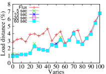
MaxMigrations = 10

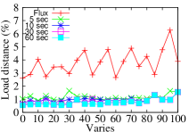
MaxMigrations = 20

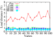
MaxMigrations = 30

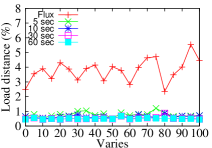
MaxMigrations = 40

Figure 2: Experimental Setting: 20 nodes, 400 key groups, 10 operators

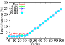
MaxMigrations = 10

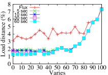
MaxMigrations = 20

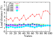
MaxMigrations = 30

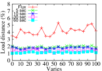
MaxMigrations = 40

Figure 3: Experimental Setting: 40 nodes, 800 key groups, 20 operators

MaxMigrations = 10

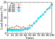
MaxMigrations = 20

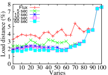
MaxMigrations = 30

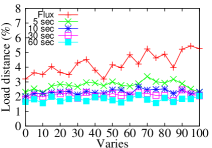
MaxMigrations = 40

Figure 4: Experimental Setting: 60 nodes, 1200 key groups, 30 operators

Hardwares. All our distributed experiments are conducted on Amazon Elastic Compute Cloud (EC2) with Apache Storm. A cluster consists of one master node, between one and four input nodes and between five and twenty worker nodes. The master node has instance type $m1.medium$, and executes the Storm master, Apache Zookeeper [17] and the Storm UI. The worker nodes have instance type $m1.medium$ and are used to execute the actual job logic. The input nodes have instance type $m3.xlarge$ and are used to produce input to the processing nodes. A few optimizer experiments are also executed locally, on a single desktop computer, with a Core i7-2600K (3.4Ghz) processor and 8G of memory, running Windows 8.1.

Initialization. As Apache Storm is based on Java, it requires an initialization phase after deployment, where the Just-In-Time compiler can do runtime optimizations. To respect this, we ignore the unstable initialization phase for each experiment, which can be seen from the missing initial time periods in our figures.

Metrics. We use load distance to measure the load imbalance. As shown in previous work [42, 22], a more balanced load distribution can be more resilient to short-term load fluctuations by minimizing the chances of overloading and the queueing latency during load spikes.

To verify the collocation of communicating key groups can reduce the system workload, we use the metric load index to measure how the system load is changed over time. It is defined as the current average system load divided by the average system load right after the initialization phase.

Techniques. The MILP (and ALBIC) is implemented using IBM ILOG CPLEX v$12.6.1$ [1] and Metis v$5.1$ [2]. In addition, all the approaches are executed with default parameters stated in the previous sections.

We compare our MILP with Flux [36] and PoTC [29], which can achieve dynamic load balancing. As Flux controls overhead by limiting the number of state migrations, we modify our MILP in the same way (i.e. we change from a limit on $maxMigrCost$ to $maxMigrations$). We also compare ALBIC with COLA [21], which, to the best of our knowledge, is the only approach that achieve similar objectives as ALBIC. As COLA is a static optimizer and does not consider runtime adaptations, invoking it for each adaptation period would incur massive state migrations. The comparison is to show how well ALBIC adapts a key group allocation plan in comparison to a complete re-optimization.

Datasets. We use three datasets for our experiments. The dataset Parsed Wikipedia edit history [5], contains the complete Wikipedia edit history up to January 2008. The data is rich with minimum $14$ attributes for each of the $116,590,856$ article revisions. The data input rate is fluctuating in the order of hundreds of tuples per second. To better illustrate the capability of our solution, we scale the size of the data, while maintaining the input distribution.

The dataset Airline On-Time [3] is provided by the Research and Innovative Technology Administration, United States Department of Transportation. We use data from the period January 2004 to December 2013, which contains information about airplanes, such as departure, arrival, expected time of arrival.

The dataset Global Surface Summary of the Day [4] is provided by the National Oceanic and Atmospheric Administration, USA. We use data from the period January 2004 to December 2013. The data contains mean temperature, mean visibility, precipitation and more, for each of the several thousand weather stations.

5.1 Solver Performance for MILP

We first investigate the relationship between solving time and solution quality for the MILP. The experiment was executed with the local desktop.

As the performance of the solver is dependent on multiple factors such as cluster size and load distribution, we use synthetic data to simulate these scenarios. Key groups are evenly allocated, such that each node has the same number of key groups. The load of each key group is initially set to the mean, which is then adjusted by a percentage, randomly chosen from the range $[-5\%,5\%]$. This is to simulate that in a realistic setting, the nodes that process these key groups have load fluctuation from one to another. Now we further adjust the load on $20\%$ of the nodes, which is controlled by a variable called varies. Half of the nodes whose load are changed gets a reduction of $0.5\cdot varies$ in their load and the other half gets an increase in load of $0.5\cdot varies$. The load changes are done by modifying the load of a randomly selected set of key groups on a node.

Figures 2 - 4 show the results of three different clusters, with varying values of maxMigrations and load fluctuations. The results show that our MILP approach consistently outperforms Flux, even after just a few seconds of optimization by the solver. The MILP approach quickly converges towards a pretty good solution (within a few seconds), which can be improved only slightly by further solving. It is only for the largest cluster considered in the experiments, that it could be benefical to solve for more than a few seconds.

Next we investigate the effect of the integration of horizontal scaling with our MILP, by comparing it with a non-integrated approach, which first performs scale-in as an independent process and then tries to move the key groups from the to-be-removed nodes to the other nodes evenly. We experiment on the largest cluster defined above. We set maxMigrations to twenty and mark ten nodes for removal. We tested two situations, where one and five nodes are overloaded (100% loaded), denoted as $1$OL and $5$OL respectively. The result in Figure 5 shows that the integrated approach obtains a good load distance much faster than the non-integrated approach for both cases, while being able to complete scaling-in within a similar time period. This is because the integrated MILP can adaptively prioritize the more urgent migrations to keep the load distance within a good range without sacrificing much on the scaling time.

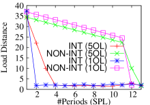
(a) Load Distance

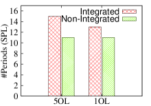
(b) Time to scale in

Figure 5: Integrating horizontal scaling with load balancing

5.2 Load Balancing with MILP

This experiment investigates the quality and overhead of load balancing which can be obtained by solving the MILP. We first provide a comparison to Flux [36] and to the “Power of Both Choices” (PoTC) [29]. Later, we evaluate the importance of limiting the overhead of the MILP. The experiment was executed on $EC2$, with one input node and twenty worker nodes. The experiment was executed on the dataset Parsed Wikipedia edit history.

Real Job 1. The job consists of one input and three operators with one hundred key groups each. The first operator calculates a GeoHash value per input tuple. The second operator calculates TopK updated articles with a window of $1$ minute and the last operator calculates global TopK updated articles, also with a window of $1$ minute. The dataset does not contain location data, so we assume a completely even distribution of GeoHash values covering Denmark.

5.2.1 Comparison with Flux and PoTC

We set $maxMigrations$ to 13 key groups per SPL, for both the MILP and Flux.

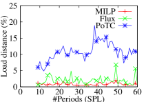
Figure 6: Quality

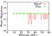
Figure 7: #Migrations

Figure 7 shows the load distances, directly after applying migrations. The MILP approach achieves a stable load distance consistently below 1%, while Flux exhibits significant fluctuations up to 7%. The reason that our approach outperforms Flux, is that Flux makes sub-optimal state migration decisions, i.e. Flux can require more state migration operations to load balance than what is necessary, meaning the maxMigrations constraint will then prevent Flux from achieving as good load balance as the MILP.

PoTC cannot achieve a consistently good load distance. This happens because the job needs to do merge (every minute) and the amount of state to merge, varies over time and from node to node. This introduces skewness in the load, which is not considered by the PoTC approach. Notice also that the PoTC approach incurs a continuous overhead to process the merging operations, regardless of the load distribution.

To recap, the benefits of our MILP is threefold: (1) it achieves better load balancing than Flux and PoTC; (2) it outperforms Flux and PoTC in terms of overhead; and (3) it can easily be adjusted by adding other constraints to support specific cases, e.g. limiting the maximum memory usage on a node.

5.2.2 Unrestricted Load Balancing

If the overhead of load balancing is not restricted, the MILP solver may potentially migrate too many key groups. To avoid this problem, the MILP has a constraint of the maximum migration cost which can be incurred per invocation. In this experiment, we investigate how the load balance “quality” and the load balance overhead, depends on this constraint (here shown as maxMigrations).

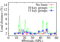
Figure 8: Quality

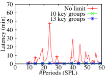
Figure 9: Overhead

Figure 9 shows the obtained load balancing is highly correlated with the number of allowed state migrations. The unrestricted solution provides the best load balance, while the one with a limit of 10 key groups provides a solution with significant spikes. Figure 9 shows that the overhead in terms of migration latency is very large for the unrestricted solution, due to a large number of key groups being migrated. The y-axis is the sum of latency incurred by all state migrations, which is defined as the amount of time that the processing of a to-be-migrated key group is paused.

Each key group to migrate incurs in average $2.5$ seconds of latency for this experiment, when migrating up to $13$ key groups at a time. Assume e.g. $SPL$ is set to five minutes, which means each of the 13 key groups to migrate, will only be paused for $\frac{2.5}{300}\cdot 100=0.8\%$ of the total time. As the experiment was executed with 300 key groups, only $\frac{2.5*13}{300\cdot 300}\cdot 100=0.04\%$ of the total processing incurs latency. Furthermore, using a more sophisticated state migration technique than direct state migration, could potentially reduce the latency to almost zero [27]. Our approach can therefore incur very low overhead on the system.

5.3 Load Balance and Collocation (Synthetic)

In this experiment we use the synthetic data and job to compare ALBIC and COLA, in terms of of load distance and collocation. The synthetic data and job are more flexible for us to generate a large topology and vary the parameters. The experimental configuration here is the same as that in Section 5.1, except that we control the maximum obtainable collocation by ensuring x% of the key groups to have 1-1 communication. Furthermore, for each iteration of solving, the load of 20% of the nodes is adjusted by a percentage, randomly chosen from the range $[-2\%,2\%]$.

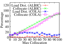
Figure 10: Collocation

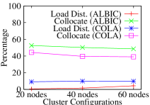
Figure 11: Configurations

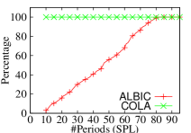
Collocation Factor

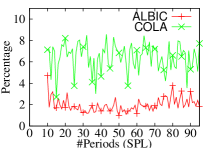
Load Distance

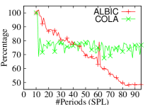
Load Index

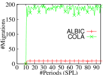
#Migrations

Figure 12: Real Job 2

Collocation Factor

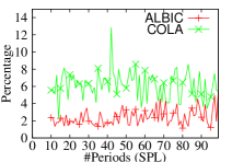
Load Distance

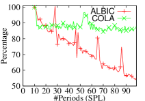
Load Index

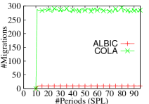
#Migrations

Figure 13: Real Job 3

Figure 11 considers a cluster of 40 nodes, 800 key groups and 20 operators. We set $maxMigrations=20$ and vary the maximum collocation factor from 0 to 100. The figure shows that ALBIC achieves a smaller, hence better, load distance than COLA. ALBIC also outperforms COLA in terms of collocation by up to ten percent. Recall that both approaches try to define partitions containing collocated key groups, while respecting some maximum load distance. The partitions must be split until the load distance requirements are satisfied by the allocation. Since ALBIC uses a much more sophisticated technique to do load balance, namely MILP, in comparison to the simple heuristic in COLA, it does not need to split partitions as much as COLA to achieve the same load distance. Therefore, it achieves better key group collocations.

In Figure 11 we set the maximum collocation factor to 50 and use the following three cluster configurations: (1) 20 nodes, 400 key groups, 10 operators; (2) 40 nodes, 800 key groups, 20 operator; and (3) 60 nodes, 1200 key groups, 30 operators. The results show that both ALBIC and COLA can achieve good solutions, while ALBIC significantly and consistently outperforms COLA in both load distance and collocation for various system sizes.

5.4 Load Balance and Collocation (Real Data)

In this experiment, we compare ALBIC and COLA with real data and realistic jobs. The experiment is executed on $EC2$, with four input node and twenty worker nodes.

Real Job 2 contains two operators, with five key groups per operator per node. The first operator extracts delays and the second operator sums delays by airplane per year. Both operators are parallelized on the same attribute. Thus, it is possible to define a perfect collocation of operators, where no data needs to be serialized and deserialized. Similarly, we can also define a worst allocation of operators, where every tuple needs to be sent over the network. The initial allocation of key groups is chosen such that the initial collocation is as little as possible, which is to see if ALBIC can gradually increase the collocation at runtime.

Figure 12 shows the collocation factor, load distance, load index and number of migrations done. As expected, COLA reaches the optimum collocation factor immediately because it optimize the plan from scratch. ALBIC, using its adaptive strategy, can gradually reach the same collocation factor over time. Furthermore, thanks to the MILP solver, ALBIC can consistently achieve a lower load distance than COLA, which adopts simple heuristics. For the load index, ALBIC gets a decrease from $100\%$ to $50\%$, which means the system load has been cut in half due to the collocation of communicating key groups. COLA can only reduce the load by $25\%$, due to the large overhead of migrations. COLA migrates close to 200 key groups per SPL, while ALBIC only migrates 10 key groups. In summary, this experiment verifies that data communication does bring a significant workload to the system and minimizing it helps rectifying system overload, and potentially save the overhead of scaling-out.

Real Job 3 extends real job 2, with an additional operator that sums delays per route, where a unique route is defined by having the same origin and destination airport. We do not consider routes that span multiple airports. To execute this experiment, the input rate for the COLA experiment is lowered to 50% (maintaining data distribution), because the overhead of migrations is simply too overwhelming for the system.

Figure 13 shows a similar trend as the previous experiment. One can see that the collocation factor is only half of the previous experiment. This is because the RouteDelay operator cannot be collocated with the SumDelay operator.

Real Job 4 extends real job 3 with several additional operators. A WeatherInput operator reads streaming input from the dataset Global Surface Summary of the Day based on the timestamps in the data. From the weatherdata we calculate a rainscore, which is a value from 0 to 100, calculated as the percentage of precipitation compared to the maximal historically measured value. The higher the rainscore, the more rain there was. The computation could be extended with a score for wind, atmospheric pressure and even thunderstorms. Each route is joined with the rainscore for a given route and the courier efficiency is calculated as the sum of delays for rainscores in intervals of ten. The store operators periodically writes results to a local relational database.

Figure 14 shows the results. For brevity, we do not show the number of migrations conducted, but it is $10$ for each iteration of ALBIC as expected. It is impossible to run COLA for each adaptation period, since the overhead of migrating key groups is too massive and exceeds the system capacity. Instead, we have executed the job three times using a random allocation without collocation and measured the collocation factor COLA achieves, which is very consistent around 61%. ALBIC gradually achieves a similar collocation factor and reduces the load index while maintaining a low load distance.

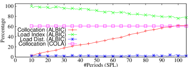
Figure 14: Real Job 4

As verified by the above experiments, both ALBIC and COLA can improve the collocation, while exhibiting a reasonable load distance at runtime. The benefit of ALBIC is twofold: (1) it incurs much less overhead at runtime and (2) it continuously and adaptively minimizes the load distance. It would be reasonable to use COLA for an initial key group allocation at job submission, and then to use ALBIC for maintaining a good allocation at runtime. If one uses a simpler load balancing algorithm such as MILP or Flux instead of ALBIC, the collocation achieved by COLA would deteriorate at runtime.

We have also studied how collocation can improve the performance of Real Job 1 described in Section 5.2. The result is that the collocation maxes out at around 5%, which is not large enough to make any conclusions on the saved workload, as the savings are masked by the load fluctuations. The collocation optimization has little effect to this job due to the way the input data of each operator is partitioned. The three partitioning functions are all independent on each other, hence they all exhibit the Full Partitioning pattern with very even distributions, which has little opportunity for collocation.

6 Conclusion

We have presented an integrated solution for load balancing, horizontal scaling and operator instance collocation suitable for general PSPEs. We first investigated how to model load balancing and dynamic scaling as an MILP, which is suitable when collocation of operator instances has little effect on the communication cost. As verified by our experiments, solving the MILP problem can achieve better load balance with a lower overhead of state migration compared to existing approaches. We then presented an extension of MILP called ALBIC, which optimizes the collocation of operator instances, while maintaining good load balancing and incurring low overhead at runtime. Our experiments verify that it maximizes the beneficial collocations without sacrificing the load balance and adaptation cost.

References

- [1] http://ibm.com/software/commerce/optimization/cplex-optimizer/index.html. Accessed: 2015-07-15.
- [2] http://glaros.dtc.umn.edu/gkhome/metis/metis/overview. Accessed: 2015-10-01.
- [3] http://apps.bts.gov/xml/ontimesummarystatistics/src/index.xml. Accessed: 2015-10-14.
- [4] https://data.noaa.gov/dataset/global-surface-summary-of-the-day-gsod. Accessed: 2016-01-05.
- [5] SNAP Datasets: Stanford large network dataset collection. http://snap.stanford.edu/data.
- [6] Y. Ahmad et al. Network awareness in internet-scale stream processing. IEEE Data Eng. Bull., 2005.
- [7] T. Akidau et al. Millwheel: Fault-tolerant stream processing at internet scale. In VLDB, 2013.
- [8] M. Balazinska et al. Fault-tolerance in the borealis distributed stream processing system. ACM TODS, 2008.
- [9] R. Castro Fernandez et al. Integrating scale out and fault tolerance in stream processing using operator state management. In SIGMOD, 2013.
- [10] T. Z. J. Fu et al. DRS: dynamic resource scheduling for real-time analytics over fast streams. ICDCS, 2015.
- [11] B. Gedik. Partitioning functions for stateful data parallelism in stream processing. VLDB, 2014.
- [12] B. Gedik et al. Elastic scaling for data stream processing. TPDS, 2013.
- [13] A. Gounaris et al. Efficient load balancing in partitioned queries under random perturbations. ACM Trans. Auton. Adapt. Syst., 2012.
- [14] V. Gulisano et al. Streamcloud: An elastic and scalable data streaming system. IEEE TPDS, 2012.
- [15] T. Heinze et al. Elastic complex event processing under varying query load. In VLDB, 2013.
- [16] B. Hindman et al. Mesos: A platform for fine-grained resource sharing in the data center. In NSDI, 2011.
- [17] P. Hunt et al. Zookeeper: wait-free coordination for internet-scale systems. In USENIXATC, 2010.
- [18] A. Ishii and T. Suzumura. Elastic stream computing with clouds. In CLOUD, 2011.
- [19] E. Kalyvianaki et al. Sqpr: Stream query planning with reuse. In ICDE, 2011.
- [20] G. Karypis and V. Kumar. Multilevel algorithms for multi-constraint graph partitioning. In SC, 1998.
- [21] R. Khandekar et al. Cola: Optimizing stream processing applications via graph partitioning. In Middleware. 2009.
- [22] C. Lei and E. A. Rundensteiner. Robust distributed query processing for streaming data. ACM TODS, 2014.
- [23] B. Li, Y. Diao, and P. Shenoy. Supporting scalable analytics with latency constraints. Proc. VLDB Endow., 2015.
- [24] J. Li et al. Out-of-order processing: A new architecture for high-performance stream systems. Proc. VLDB Endow., 2008.
- [25] J. Li et al. Minimizing communication cost in distributed multi-query processing. In ICDE, 2009.
- [26] K. G. S. Madsen et al. Integrating fault-tolerance and elasticity in a distributed data stream processing system. In SSDBM, 2014.
- [27] K. G. S. Madsen and Y. Zhou. Dynamic resource management in a massively parallel stream processing engine. In CIKM, 2015.
- [28] J. B. Mazzola et al. Heuristics for the multi-resource generalized assignment problem. Naval Research Logistics, 2001.
- [29] M. A. U. Nasir et al. The power of both choices: Practical load balancing for distributed stream processing engines. In ICDE, 2015.
- [30] L. Neumeyer et al. S4: Distributed stream computing platform. In ICDMW, 2010.
- [31] B. Overeinder et al. A dynamic load balancing system for parallel cluster computing. Future Generation Computer Systems, 1996.
- [32] P. Pietzuch et al. Network-aware operator placement for stream-processing systems. In ICDE, 2006.
- [33] N. Rivetti et al. Efficient key grouping for near-optimal load balancing in stream processing systems. In DEBS, 2015.
- [34] K. W. Ross and D. D. Yao. Optimal load balancing and scheduling in a distributed computer system. Journal of the ACM, 1991.
- [35] B. Satzger et al. Esc: Towards an Elastic Stream Computing Platform for the Cloud. In CLOUD, 2011.
- [36] M. A. Shah et al. Flux: An adaptive partitioning operator for continuous query systems. In ICDE, 2003.
- [37] I. Stanoi et al. Whitewater: Distributed processing of fast streams. TKDE, 2007.
- [38] A. Toshniwal et al. Storm@twitter. In SIGMOD, 2014.
- [39] J. Wolf et al. Soda: An optimizing scheduler for large-scale stream-based distributed computer systems. In Middleware. 2008.
- [40] Y. Wu and K.-L. Tan. Chronostream: Elastic stateful stream computation in the cloud. In ICDE, 2015.
- [41] Y. Xing et al. Dynamic load distribution in the borealis stream processor. In ICDE, 2005.
- [42] Y. Xing et al. Providing resiliency to load variations in distributed stream processing. In VLDB, 2006.
- [43] M. Zaharia et al. Discretized streams: Fault-tolerant streaming computation at scale. In SOSP, 2013.
- [44] J. Zhou et al. Advanced partitioning techniques for massively distributed computation. In SIGMOD, 2012.
- [45] Y. Zhou et al. Efficient dynamic operator placement in a locally distributed continuous query system. In OTM. 2006.