A public code for general relativistic, polarised radiative transfer around spinning black holes

Abstract

Ray tracing radiative transfer is a powerful method for comparing theoretical models of black hole accretion flows and jets with observations. We present a public code, grtrans, for carrying out such calculations in the Kerr metric, including the full treatment of polarised radiative transfer and parallel transport along geodesics. The code is written in Fortran 90 and efficiently parallelises with OpenMP, and the full code and several components have Python interfaces. We describe several tests which are used for verifiying the code, and we compare the results for polarised thin accretion disc and semi-analytic jet problems with those from the literature as examples of its use. Along the way, we provide accurate fitting functions for polarised synchrotron emission and transfer coefficients from thermal and power law distribution functions, and compare results from numerical integration and quadrature solutions of the polarised radiative transfer equations. We also show that all transfer coefficients can play an important role in predicted images and polarisation maps of the Galactic center black hole, Sgr A*, at submillimetre wavelengths.

1 Introduction

Quantitative comparisons of theoretical models of black hole accretion flows and jets with observations require radiative transfer calculations. The bulk of the radiation is often produced near the black hole event horizon, where relativistic effects of Doppler beaming, gravitational redshift, and light bending become important. Ray tracing is a convenient method for carrying out fully relativistic radiative transfer calculations. Light bending is naturally accounted for by taking the rays to be null geodesics in the Kerr metric, and the radiative transfer equation can then be solved along geodesics to calculate observed intensities.

This technique has been used to calculate images (e.g., Luminet, 1979) and spectra (e.g., Cunningham, 1975) of thin black hole accretion discs (Shakura & Sunyaev, 1973; Page & Thorne, 1974), including state of the art methods to fit spectra in order to infer parameters such as the black hole spin (Davis & Hubeny, 2006; Li et al., 2005; Dauser et al., 2010). Ray tracing is also convenient for including general relativistic rotations of the polarisation direction via parallel transport (Connors & Stark, 1977; Connors, Stark & Piran, 1980), and has been applied to the polarised radiative transfer of synchrotron radiation from thick accretion discs, e.g. in order to model the Galactic center black hole Sgr A* (Broderick & Loeb, 2005, 2006). With the development of general relativistic MHD simulations of black hole accretion (De Villiers & Hawley, 2003; Gammie, McKinney & Tóth, 2003), ray tracing has become popular as a post-processing step to study their variability properties (Schnittman, Krolik & Hawley, 2006; Noble & Krolik, 2009; Dexter & Fragile, 2011) and radiative efficiency (Noble et al., 2011; Kulkarni et al., 2011), as well as for comparison with observations of Sgr A* (e.g., Noble et al., 2007; Mościbrodzka et al., 2009; Dexter, Agol & Fragile, 2009; Chan et al., 2015; Gold et al., 2016) and M87 (e.g., Dexter, McKinney & Agol, 2012; Moscibrodzka, Falcke & Shiokawa, 2015).

Of particular interest are radiative transfer calculations relevant for current and future event horizon scale interferometric observations of Sgr A* and M87 at submillimeter (The Event Horizon Telescope, Doeleman et al., 2009) and near-infrared (the VLTI GRAVITY instrument, Eisenhauer et al., 2008) wavelengths. Fully modeling the observed synchrotron radiation requires polarised radiative transfer. Existing codes for this application are either private (Broderick & Blandford, 2004) or written as post-processors to specific numerical simulations (Shcherbakov, Penna & McKinney, 2012). Other public tools (e.g., Gyoto and Kertap, Vincent et al., 2011; Chen et al., 2015) do not include fully polarised radiative transfer.

We present a publicly available, fully general relativistic code, grtrans, for polarised radiative transfer via ray tracing in the Kerr metric. We describe the methods used for the parallel transport of the polarisation basis into the local frame of the fluid (§2.2) and the integration of the polarised radiative transfer equations (§2.5) using emission, absorption, and rotation coefficients (§2.3) calculated based on radiative processes in terms of a background fluid model (§2.4). In §3, we discuss tests used to validate the code, and comparisons of full example problems to those in the literature. We also provide fitting functions for polarised synchrotron emission, absorption, and transfer coefficients (Appendix B and B), and show an example polarised image from a model of the submm emission of Sgr A*, to demonstrate how all of the transfer coefficients play important roles in the final polarised image. Finally, §4 gives a summary of the code convergence and performance properties, and an overview of its organisation.

2 Methods

The goal of a ray tracing radiative transfer code is to calculate the observed intensity on locations (pixels) of an observer’s camera for a given model of emission and absorption. We calculate the Boyer-Lindquist coordinates of the photon trajectories from the observer towards the black hole (trace the rays) corresponding to each pixel, parallel transport the observed polarisation basis into the fluid frame, calculate the local emission and absorption properties at each location, and then solve the radiative transfer equations for the given emission and abosrption along those rays.

2.1 Ray tracing

The observer’s camera at inclination $\mu_{0}=\cos{\theta_{0}}$ and orientation $\phi_{0}$ has pixels whose coordinates are described by apparent impact parameters $\alpha$, $\beta$ parallel and perpendicular to the black hole spin axis. The photon trajectories in grtrans are assumed to be geodesics in the Kerr metric, in which case their constants of motion are specified for given $\alpha$, $\beta$ (Bardeen, Press & Teukolsky, 1972):

$$l=-\alpha\sqrt{1-\mu_{0}^{2}},$$ (1)

$$q^{2}=\beta^{2}+\mu_{0}^{2}(\alpha^{2}-a^{2}),$$ (2)

where $l$, $q^{2}$, and $a$ are the dimensionless z-component of the angular momentum, Carter’s constant, and black hole spin parameters.

The trajectories for each ray given the constants can then be found by solving the geodesic equation. We do this semi-analytically by reducing the equations of motion to Jacobian integrals and Jacobi-elliptic functions (Rauch & Blandford, 1994; Agol, 1997) as implemented in the code geokerr (Dexter & Agol, 2009).

In this method, the independent variable is either the inverse radius $u=1/r$ or $\mu=\cos{\theta}$. The former is used by default, since even steps in $u$ naturally concentrate resolution towards the black hole, where most of the radiation is produced. In special cases, for example a thin accretion disc in the equatorial plane, the latter method is preferable since then one can solve for the radius where $\mu=0$, without needing to integrate the geodesic. In the default case with $u$ as the independent variable, the sampling can become poor near radial turning points (e.g. sections of the orbit at nearly constant radius). For this reason, near radial turning points $\mu$ is instead used as the independent variable to fill in the geodesic.

The calculation is started at a small, non-zero value of $u$ in order to keep the coordinate time and affine parameter finite. The geodesics are tabulated starting at a value of $u$ of interest for the problem (e.g. the outer radial boundary of a numerical simulation) and are terminated either just outside the event horizon for bound orbits, or once they again reach the outer radius of interest for the calculation. The locations to sample ($u_{i}$) and number of samples ($n$) are code parameters. The assumption made by the code is that the initial intensity is zero at the farthest point sampled along the ray.

2.2 Parallel transport of the polarisation basis

The observed polarisation is measured with respect to the horizontal and vertical axes defining the camera, while the polarised emission and transfer coefficients are most naturally given relative to a local direction in the emitting fluid (e.g. the magnetic field direction for synchrotron radiation). To relate the two, we first parallel transport the observed polarisation basis along the geodesic, and then transform it to the orthonormal frame comoving with the fluid. The angle between the two bases can then be used to rotate the local coefficients into the observed polarisation basis.

Parallel transport of a vector describing the polarisation basis $f^{\mu}$ perpendicular to the wave-vector $k^{\mu}$ is simplified in the Kerr metric by the existence of of a complex constant called the Walker-Penrose constant (Walker & Penrose, 1970), given in Boyer-Lindquist coordinates with $G=c=M=1$ as (Connors & Stark, 1977; Connors, Stark & Piran, 1980; Chandrasekhar, 1983):

$$K_{1}-iK_{2}=(r-ia\cos{\theta})\left\{(k^{t}f^{r}-k^{r}f^{t})+a\sin^{2}{\theta}(k^{r}f^{\phi}-k^{\phi}f^{r})\right.$$

$$\left.-i[(r^{2}+f^{2})(k^{\phi}f^{\theta}-f^{\phi}k^{\theta})-a(k^{t}f^{\theta}-k^{\theta}f^{t})]\sin{\theta}\right\},$$ (3)

where

$$k^{t} = \frac{1}{\rho^{2}}\left[-a\left(a\sin^{2}{\theta}-l\right)+\frac{\left(r^{2}+a^{2}\right)}{\Delta}\left(r^{2}+a^{2}-al\right)\right],$$ (4)

$$k^{r} = -\frac{s_{r}}{\rho^{2}}R(r),$$ (5)

$$k^{\theta} = -\frac{s_{\theta}}{\rho^{2}}\sqrt{\frac{M(\theta)}{\sin^{2}{\theta}}},$$ (6)

$$k^{\phi} = \frac{1}{\rho^{2}}\left[-a+\frac{l}{\sin^{2}{\theta}}+\frac{a}{\Delta}(r^{2}+a^{2}-al)\right],$$ (7)

$$M(\theta) = q^{2}+\left(a^{2}-q^{2}-l^{2}\right)\cos^{2}{\theta}-a^{2}\cos^{4}{\theta},$$ (8)

$$R(r) = r^{2}+(a^{2}-q^{2}-l^{2})+2\left[(a-l)^{2}+q^{2}\right]r^{-1}$$ (9)

$$- a^{2}q^{2}r^{-2},$$ (10)

$$\rho^{2} = r^{2}+a^{2}\cos^{2}{\theta},$$ (11)

$$\Delta = r^{2}-2r+a^{2},$$ (12)

is the photon wave vector whose direction is specified by the signs $s_{r}$ and $s_{\theta}$ (e.g., Rauch & Blandford, 1994).

The real and imaginary parts of the constant, $K_{1}$ and $K_{2}$, provide two constraints on the transported basis vectors, while the orthogonality condition $k^{\mu}f_{\mu}=0$ provides a third. Since the polarisation basis vectors are already only defined up to a multiple of the wave vector, we can set $f^{t}=0$ without any loss of generality, which leaves three linear equations for the three remaining components of $f^{\mu}$:

$$K_{1} = \delta_{1}f^{r}+\delta_{2}f^{\theta}+\delta_{3}f^{\phi}$$ (14)

$$K_{2} = \gamma_{1}f^{r}+\gamma_{2}f^{\theta}+\gamma_{3}f^{\phi}$$ (15)

$$k^{\mu}a_{\mu} = 0$$ (16)

with

$$\delta_{1} = rk^{t}-ra\sin^{2}{\theta}k^{\phi}$$ (17)

$$\delta_{2} = a^{2}\sin{\theta}\cos{\theta}k^{t}-a\cos{\theta}\sin{\theta}(r^{2}+a^{2})k^{\phi}$$ (18)

$$\delta_{3} = ra\sin^{2}{\theta}k^{r}+a\cos{\theta}\sin{\theta}(r^{2}+a^{2})k^{\theta}$$ (19)

$$\gamma_{1} = a\cos{\theta}k^{t}-a^{2}\cos{\theta}\sin^{2}{\theta}k^{\phi}$$ (20)

$$\gamma_{2} = r(r^{2}+a^{2})\sin{\theta}k^{\phi}-ar\sin{\theta}k^{t}$$ (21)

$$\gamma_{3} = a^{2}\cos{\theta}\sin^{2}{\theta}k^{r}-r(r^{2}+a^{2})\sin{\theta}k^{\theta}.$$ (22)

The components of $f^{\mu}$ can then be calculated as:

$$f^{r} = \frac{1}{N}\left[(\gamma_{2}K_{1}-\delta_{2}K_{2})(g_{\phi\phi}k^{\phi}+g_{\phi t}k^{t})-\right.$$ (24)

$$\left.(\gamma_{3}K_{1}-\delta_{3}K_{2})g_{\theta\theta}k^{\theta}\right],$$

$$f^{\theta} = -\frac{1}{N}\left[(\gamma_{1}K_{1}-\delta_{1}K_{2})(g_{\phi\phi}k^{\phi}+g_{\phi t}k^{t})-\right.$$ (26)

$$\left.(\gamma_{3}K_{1}-\delta_{3}K_{2})g_{rr}k^{r}\right],$$

$$f^{\phi} = \frac{1}{N}\left[(\gamma_{1}K_{1}-\delta_{1}K_{2})g_{\theta\theta}k^{\theta}-\right.$$ (28)

$$\left.(\gamma_{2}K_{1}-\delta_{2}K_{2})g_{rr}k^{r}\right],$$

$$N = (\gamma_{2}\delta_{1}-\gamma_{1}\delta_{2})g_{\phi\phi}k^{\phi}-(\gamma_{3}\delta_{1}-\gamma_{1}\delta_{3})g_{\theta\theta}k^{\theta}$$ (29)

$$+ (\gamma_{2}\delta_{1}-\gamma_{1}\delta_{2})g_{\phi t}k^{t}+(\gamma_{3}\delta_{2}-\gamma_{2}\delta_{2})g_{rr}k^{r},$$

where $g_{\mu\nu}$ are the covariant metric components:

$$g_{tt} = -\frac{1}{\rho^{2}\Delta}\left[\left(r^{2}+a^{2}\right)^{2}-a^{2}\Delta\sin^{2}{\theta}\right],$$ (30)

$$g_{\phi t} = \frac{-2ar\sin^{2}{\theta}}{\rho^{2}},$$ (31)

$$g_{rr} = \frac{\rho^{2}}{\Delta},$$ (32)

$$g_{\theta\theta} = \rho^{2},$$ (33)

$$g_{\phi\phi} = \frac{\Sigma\sin^{2}{\theta}}{\rho^{2}},$$ (34)

$$\Sigma = (r^{2}+a^{2})^{2}-a^{2}\Delta\sin^{2}{\theta}.$$ (35)

The polarisation basis at the camera is defined so that positive Stokes Q is measured relative to the $\hat{\phi}_{0}$ axis. Transforming the linear polarisation basis vectors $\hat{\phi}_{0}$ and $\hat{\theta}_{0}$ at the camera then requires knowledge of $K_{1}$ and $K_{2}$ for these vectors. These can be found from the asymptotic form of equation (2.2) (Chandrasekhar, 1983). They are given by $K_{1}=-\gamma$, $K_{2}=-\beta$ and $K_{1}=-\beta$, $K_{2}=\gamma$ respectively, where $\gamma=-\alpha-a\sin{\theta}_{0}$ (Connors, Stark & Piran, 1980). Then equations (24-29) allow us to calculate the polarisation basis vectors at any point along the ray.

2.2.1 Transformation to the orthonormal fluid frame

The emission coefficients and the transfer matrix computed in the fluid frame are defined in a basis aligned with a local reference vector. For the case of synchrotron emission, it is convenient to use the local magnetic field direction and so we use $b^{\mu}$ as this vector in grtrans without loss of generality. In the case of electron scattering in a thin accretion disc, the polarisation is given relative to the disc normal vector, and so we assign the variable $b^{\mu}$ to that vector.

Before integrating the radiative transfer equations, these coefficients must be transformed to the observed polarisation basis. This transformation requires finding the angle between the transported polarisation basis vectors and the polarisation reference vector (Shcherbakov & Huang, 2011). We transform into the orthonormal frame comoving with the fluid where the four-velocity is $\hat{u}^{\mu}=(1,0,0,0)$. The basis four-vectors of the transformation are (Krolik, Hawley & Hirose, 2005; Beckwith, Hawley & Krolik, 2008; Shcherbakov & Huang, 2011; Kulkarni et al., 2011):

$$e^{\mu}_{(t)} = u^{\mu},$$ (36)

$$e^{\mu}_{(r)} = (u_{r}u^{t},-(u_{t}u^{t}+u_{\phi}u^{\phi}),0,u_{r}u^{\phi})/N_{r},$$ (37)

$$e^{\mu}_{(\theta)} = (u_{\theta}u^{t},u_{\theta}u^{r},1+u_{\theta}u^{\theta},u_{\theta}u^{\phi})/N_{\theta},$$ (38)

$$e^{\mu}_{(\phi)} = (u_{\phi},0,0,-u_{t})/N_{\phi},$$ (39)

where the upper (lower) indices are lowered (raised) with the Kerr (Minkowski) metric and,

$$N^{2}_{r} = -g_{rr}(u_{t}u^{t}+u_{\phi}u^{\phi})(1+u_{\theta}u^{\theta}),$$ (40)

$$N^{2}_{\theta} = g_{\theta\theta}(1+u_{\theta}u^{\theta}),$$ (41)

$$N^{2}_{\phi} = -(u_{t}u^{t}+u_{\phi}u^{\phi})\Delta\sin^{2}{\theta},$$ (42)

$$\Delta = r^{2}-2r+a^{2}.$$ (43)

Four-vectors in the coordinate frame are transformed as,

$$A_{(\alpha)}=e^{\mu}_{(\alpha)}A_{\mu}.$$ (44)

The angle $\chi$ between the projected magnetic field and the polarisation basis is given in terms of ordinary dot products of the magnetic field and parallel-transported basis three-vectors (denoted by hats):

$$\sin{2\chi} = -2\frac{\left(\hat{a}\cdot\hat{B}\right)\left(\hat{b}\cdot\hat{B}\right)}{\left(\hat{a}\cdot\hat{B}\right)^{2}+\left(\hat{b}\cdot\hat{B}\right)^{2}},$$ (45)

$$\cos{2\chi} = \frac{\left(\hat{b}\cdot\hat{B}\right)^{2}-\left(\hat{a}\cdot\hat{B}\right)^{2}}{\left(\hat{a}\cdot\hat{B}\right)^{2}+\left(\hat{b}\cdot\hat{B}\right)^{2}}.$$ (46)

In this frame, the combined redshift and Doppler factor $g\equiv\nu_{0}/\nu=-1/\hat{k}^{t}$ and $\cos\theta_{B}={\frac{\hat{k}\cdot\hat{B}}{|\hat{k}||\hat{B}|}}$.

2.2.2 Transfer Equation

The non-relativistic polarised radiative transfer equation can be written in the form,

$$\frac{d}{ds}\left(\begin{array}[]{c}I\\ Q\\ U\\ V\\ \end{array}\right)=\left(\begin{array}[]{c}j_{I}\\ j_{Q}\\ j_{U}\\ j_{V}\end{array}\right)-\left(\begin{array}[]{cccc}\alpha_{I}&\alpha_{Q}&\alpha_{U}&\alpha_{V}\\ \alpha_{Q}&\alpha_{I}&\rho_{V}&\rho_{U}\\ \alpha_{U}&-\rho_{V}&\alpha_{I}&\rho_{Q}\\ \alpha_{V}&-\rho_{U}&-\rho_{Q}&\alpha_{I}\\ \end{array}\right)\left(\begin{array}[]{c}I\\ Q\\ U\\ V\\ \end{array}\right)$$ (47)

where ($I$, $Q$, $U$, $V$) are the Stokes parameters, $j_{I,Q,U,V}$ are the polarised emissivities, $\alpha_{I,Q,U,V}$ are the absorption coefficients, and $\rho_{Q,U,V}$ are the Faraday rotation and conversion coefficients.

In the context of synchrotron radiation, the transfer equation can be simplified by aligning the magnetic field with Stokes $U$, so that $j_{U}=\alpha_{U}=\rho_{U}=0$. Then $j_{Q}$, $\alpha_{Q}$ ($j_{V}$, $\alpha_{V}$) correspond to the emission and absorption coefficients for linear (circular) polarisation and $j_{I}$, $\alpha_{I}$ are the unpolarised coefficients. The transfer coefficients $\rho_{Q,V}$ describe the effects of Faraday conversion and rotation respectively.

All coefficients are computed in the fluid rest frame, where $\nu$ is the emitted frequency, related to the observed frequency through $g$. Then the transfer equation is recast into invariant form: $\mathcal{I}=g^{3}\mathbf{I}$, $\mathcal{J}=g^{2}\mathbf{j}$, and $\mathcal{K}=g^{-1}\mathbf{K}$, where $\mathbf{I}$, $\mathbf{j}$ and $\mathbf{K}$ are the intensity and emissivity vectors and the transfer matrix from equation (47).

Finally, we use the angle $\chi$ to rotate the emissivity and absorption matrix in the fluid frame into that of the observer, such that the radiative transfer equation becomes,

$$\frac{d\mathcal{I}}{d\lambda}=\hat{\mathcal{J}}-\hat{\mathcal{K}}\mathcal{I},$$ (48)

where $\lambda$ is an affine parameter, $\hat{\mathcal{J}}=g^{2}R(\chi)\mathbf{j}$, $\hat{\mathcal{K}}=g^{-1}R(\chi)\mathbf{K}R(-\chi)$, and

$$R(\chi)=\left(\begin{array}[]{cccc}1&0&0&0\\ 0&\cos{2\chi}&-\sin{2\chi}&0\\ 0&\sin{2\chi}&\cos{2\chi}&0\\ 0&0&0&1\\ \end{array}\right).$$ (49)

This rotation transforms the fluid frame polarisation basis to that at infinity, including the parallel transport of the polarisation four-vector along the ray.

Equation 48 includes all relativistic effects. The bending of light is accounted for by the calculation of null geodesics (Dexter & Agol, 2009), the gravitational redshifts and Doppler shifts due to fluid motions are included in $g$.

This method, developed by Shcherbakov & Huang (2011), parallel transports the polarisation basis along the ray and into the fluid frame. This is similar to the approach of Connors, Stark & Piran (1980), who transported a local polarisation vector $f^{\mu}$ from the fluid to the observer. Gammie & Leung (2012) derived a general formalism for covariant polarised radiative transfer, and mathematically showed the equivalence of the approach used here and alternative methods used by Broderick & Blandford (2004) and Schnittman & Krolik (2013). We show tests and example problems comparing results from these methods in §3.3.

2.3 Transfer coefficients

The transfer coefficients in equation (47) depend in general on the physical properties of the radiating particles. Here we focus specifically on the case of synchrotron radiation appropriate for studying accretion flows at the lowest observed luminosities (e.g., Sgr A*). Adding different emissivities such as bremsstrahlung to grtrans would require a straightforward modification of the code.

In addition, the form of the transfer coefficients depends on the underlying electron distribution function. The appropriate forms for thermal and power law distributions are implemented in the code. More general distribution functions can be built by combining these components (e.g. a thermal distribution with a power law “tail” or a superposition of thermal distributions, Mao et al. in prep.). In these special cases, the integral over the distribution function can be analytically approximated to high accuracy in the ultra-relativistic synchrotron limit (e.g., Mahadevan, Narayan & Yi, 1996). The full forms for the transfer coefficients as used in grtrans and some of their derivations are given in Appendix A.

In addition to synchrotron coefficients, for test problems with optically thick accretion discs the code uses (color-corrected) blackbody intensity functions for the disc surface brightness.

2.4 Fluid models

The calculation of transfer coefficients for a particular emission model requires knowledge of the fluid state variables of spacetime coordinates. Depending on the model used, this can include the electron density, magnetic field strength and orientation, and the internal energy density in electrons. In grtrans we implement several fluid models from the literature. They are described briefly below, and used as code examples and tests in §3.3.

2.4.1 Thin accretion discs

The relativistic version (Page & Thorne, 1974) of the standard thin disc solution (Shakura & Sunyaev, 1973) for axisymmetric, steady accretion in the equatorial plane is implemented and intended for use with a model for the emergent intensity from the disc (e.g., a blackbody). In this case, the net polarisation is taken to follow the result of electron scattering in a semi-infinite atmosphere (Sobolev, 1963; Chandrasekhar, 1950) specified relative to the disc normal vector (§3.1).

2.4.2 Alternative thin accretion discs

We have also implemented a numerical version of the thin accretion disc problem which inputs a temperature distribution $T(r,\phi)$ in the equatorial plane. One example use of this is for calculating spectra of inhomogeneous (or “patchy") accretion discs (Dexter & Agol, 2011), as used for the polarisation calculations described in Dexter & Quataert (2012).

2.4.3 Spherical accretion flow

A solution of the general relativistic fluid equations for spherically symmetric inflow in the Schwarzschild metric following (Michel, 1972; Shapiro, 1973a) is implemented. The dominant emission in this case comes from synchrotron radiation (Shapiro, 1973b). See Dexter & Agol (2009) for details.

For polarised emission, we take the magnetic field to be purely radial. This is done to check that the resulting linear polarisation sums to zero (since for a camera centered on the black hole there is no preferred direction), and the residual is used as an estimate of the minimum systematic uncertainty in the fractional linear polarisation ($\simeq 0.01\%$).

2.4.4 Semi-analytic jet model

Broderick & Loeb (2009) presented a semi-analytic jet model based on stream functions found in force-free simulations. We have implemented this solution numerically on a grid of ($r$,$\theta$) in Boyer-Lindquist coordinates. To generate our numerical solutions, we solve for the magnetic field and velocity structure analytically using their equations 5-13. To get the particle density, we tabulate their function $F(\psi)$ numerically using a separate grid of points with roughly constant $z\simeq r_{\rm fp}$ and varying $\psi=r^{2-2\xi}(1-\cos{\theta})$. This function can then be used to calculate the particle density (their equation 13).

The fluid variable solutions from our method appear identical to what is shown in their Figure 4.

2.4.5 Numerical general relativistic MHD solution

We also use another numerical solution, from the public version of the axisymmetric general relativistic MHD code HARM (Gammie, McKinney & Tóth, 2003; Noble et al., 2006). Starting from a gas torus in hydrostatic equlibrium threaded with a weak magnetic field, the code evolves the equations of ideal MHD in the Kerr spacetime. The magnetorotational instability (Balbus & Hawley, 1991) drives turbulence in the torus and the resulting stresses transport angular momentum outwards, leading to accretion onto the central black hole. Snapshots from these simulations have been used as models of Sgr A* (e.g., Noble et al., 2007; Mościbrodzka et al., 2009).

The images used here as examples are from a single snapshot of a simulation with black hole spin $a=0.9375$ at $t=2000GM/c^{3}$ used for comparison with 3D simulations in Dexter et al. (2010). grtrans supports fully time-dependent calculations using a series of such simulation snapshots to e.g. calculate accretion flow movies rather than images. It would also be straightforward to adapt the code to work with updated HARM versions, for example with 3D data or non-ideal MHD.

The fluid variables in these simulations are saved in modified Kerr-Schild coordinates and with arbitrary units which assume $G=c=M=1$. Calculating radiation from these data in grtrans requires converting to Boyer-Lindquist coordinates and to cgs units. The coordinate conversion is done analytically in two steps: from modified to standard Kerr-Schild coordinates (Gammie, McKinney & Tóth, 2003) and then from Kerr-Schild to Boyer-Lindquist coordinates (e.g., Font, Ibáñez & Papadopoulos, 1999). Scaling to cgs units is done by i) fixing the black hole mass, which sets the length- and time-scales, and ii) choosing an average accretion rate (or equivalently mass of the initial torus). This procedure is discussed in more detail elsewhere (Schnittman, Krolik & Hawley, 2006; Noble et al., 2007; Dexter et al., 2010).

Once the unit and coordinate conversions are done, we calculate fluid variables at tabulated geodesic coordinates. For all numerical models, we linearly interpolate from the set of nearest neighbors on the grid for the numerical model. The way this is implemented in the code assumes that the grid is uniformly spaced in some coordinates, and the fluid model must include the transformation from those coordinates to Boyer-Lindquist.

There are several other models implemented in the code in some form, but which have not been tested. It is straightforward to add new fluid models to the code, e.g. by using existing ones as templates.

2.5 Integration of the polarised radiative transfer equations

From the previous steps, we have transfer coefficients specified at tabulated points along a geodesic which are transformed to relativistic invariant form and aligned with the observed Stokes parameters of the distant observer, accounting for parallel transport along each ray.

The final step is to solve the polarised radiative transfer (equation 48) along the geodesic. In grtrans, this is done as a separate step following the calculation of the coordinates of the geodesic. While the ray tracing proceeds backwards from the camera towards the black hole, the integration proceeds outwards. This is done so that we may safely set the initial intensity to zero at some point either where the optical depth is large, or where the geodesic has left the emitting volume. Here we describe one numerical integration method and two quadrature methods that are implemented in grtrans for integrating the equations.

These methods can be used for relativistic or non-relativistic problems. For consistency with previous literature, we write the non-relativistic versions of the intensity, absorption matrix, emissivity, and step size along the ray at index $k$ as $I_{k}$, $K_{k}$, $j_{k}$ and $\Delta s_{k}$ in what follows. In grtrans, the relativistic invariants $\mathcal{I}(\lambda_{k})$, $\hat{\mathcal{K}}(\lambda_{k})$, $\hat{\mathcal{J}}(\lambda_{k})$, and $\Delta\lambda_{k}$ take the place of these quantities.

2.5.1 Numerical integration

The most straightforward method is numerical integration of the radiative transfer equation. The radiative transfer equations can be stiff: the required step size for a converged solution decreases sharply once $\tau\gtrsim 1$, where $\tau$ is the optical depth associated with any transfer coefficient.

In order to get a robust solution, we use the ODEPACK routine LSODA (Hindmarsh, 1983) to advance the Stokes intensities between each step tabulated on the geodesic. This algorithm adaptively switches between a predictor-corrector (Adams) method for non-stiff systems, and a BDF method for stiff systems. We find it necessary to restrict the maximum step size allowed in $\lambda$, since otherwise a large step can miss the region of interest altogether.

Regions of large optical depth often contribute negligibly to the observed intensity but require a small step size, and so we terminate the integration at a maximum optical depth, $\tau_{max}=10$ by default. There are further free parameters in LSODA related to the error tolerance.

The locations sampled by LSODA do not correspond exactly to the points tabulated along the ray. We linearly interpolate the transfer coefficients between tabulated points, even though they are highly non-linear functions of position along the geodesic. The fluid variables vary more smoothly along the ray, and it would be straightforward but more computationally expensive to instead re-interpolate the fluid variables to the points used by LSODA and then calculate new transfer coefficients, as was done in the previous version of the code (Dexter, 2011). Given the results from comparing to quadrature integration methods and analytic solutions described below, and from the convergence properties with increasing the number of points along each ray, we find the current approximation adequate for obtaining accurate solutions.

2.5.2 Quadrature solutions

The polarised radiative transfer equations are linear and ordinary, and so admit a formal solution analagous to that of the unpolarised case (Rybicki & Lightman, 1979). The solution amounts to finding the matrix operator $\mathbf{O}(s,s^{\prime})$, defined by (Landi Degl’Innocenti & Landi Degl’Innocenti, 1985),

$$\frac{d}{ds}\mathbf{O}(s,s^{\prime}) = -\mathbf{K}(s)\mathbf{O}(s,s^{\prime}),$$ (50)

$$\mathbf{O}(s,s) = \mathbf{1},$$ (51)

which determines how the intensity is propagated over some part of the ray in the absence of emission. In the unpolarised case this is a scalar, $O=\exp{[-(\tau(s)-\tau(s^{\prime})]}$. If the absorption matrix $\mathbf{K}$ is a constant over the ray, then similarly,

$$\mathbf{O}(s,s^{\prime})=\exp{[-\mathbf{K}(s-s^{\prime})]}.$$ (52)

In terms of $\mathbf{O}$, the intensity can be written in terms of an initial value $I_{n-1}(s_{n-1})$:

$$\mathbf{I}(s)=\int_{s_{n-1}}^{s}ds^{\prime}\mathbf{O}(s,s^{\prime})j(s^{\prime})+\mathbf{O}(s,s_{n-1})I_{n-1}.$$ (53)

Landi Degl’Innocenti & Landi Degl’Innocenti (1985) found a closed form solution for $\mathbf{O}$ (their equation 10, reproduced in Appendix D). This solution is valid for regions where the transfer matrix $\mathbf{K}$ is constant, but not for our situation of interest where they vary arbitrarily along a ray. In order to use this expression, we assume that the coefficients are constant in between the tabulated locations along a geodesic starting from $s_{k=n}$ at the farthest point of interest along the ray (at the black hole or where the ray leaves the far end of the emitting region) and integrating towards $s_{k=0}$ (the “surface”), and write the solution of equation (53) separately for the interval between neighboring points with indices $k+1$ and $k$ with positions $s_{k+1}$ and $s_{k}$:

$$I_{k}=O_{k,k+1}j_{k}\Delta s_{k}+O_{k,k+1}I_{k+1},$$ (54)

where $\Delta s_{k}=s_{k+1}-s_{k}$. This formula is used recursively going outwards from $s_{n-1}$ to $s_{0}$ to find the intensity everywhere from the initial condition $I_{n-1}=0$.

The final integration method implemented in grtrans is the diagonal element lambda operator method (DELO, Rees, Durrant & Murphy, 1989), which comes from writing the transfer equations in terms of the unpolarised optical depth, $d\tau=\alpha_{I}ds$, and the modified absorption matrix $K^{\prime}=\mathbf{K}/\alpha_{I}-\mathbf{1}$ and source function $S^{\prime}=\mathbf{j}/\alpha_{I}$:

$$\frac{d\mathbf{I}}{d\tau}=\mathbf{I}-\mathcal{S},$$ (55)

where $\mathcal{S}=S^{\prime}-K^{\prime}\mathbf{I}$. This equation has a formal solution between neighbouring points $\tau_{k+1}$, $\tau_{k}$ of

$$I(\tau_{k})=E_{k}I(\tau_{k+1})+\int_{\tau_{k}}^{\tau_{k+1}}\exp[-(\tau-\tau_{k})]\mathcal{S}d\tau,$$ (56)

where $E_{k}=\exp(-\delta_{k})$ and $\delta_{k}=\tau_{k+1}-\tau_{k}$. The DELO method makes a linear approximation for the modified source function,

$$\mathcal{S}(\tau)=[(\tau_{k+1}-\tau)\mathcal{S}_{k}+(\tau-\tau_{k})\mathcal{S}_{k+1}]/\delta_{k},$$ (57)

so that equation (56) can be integrated analytically between grid points, giving:

$$I(\tau_{k})=\mathcal{P}_{k}+\mathcal{Q}_{k}I(\tau_{k+1}),$$ (58)

where

$$\mathcal{P}_{k} = \mathcal{M}_{k}[(F_{k}-G_{k})S^{\prime}_{k}+G_{k}S^{\prime}_{k+1}],$$ (59)

$$\mathcal{Q}_{k} = \mathcal{M}_{k}(E_{k}\mathbf{1}-G_{k}K^{\prime}_{k+1}),$$ (60)

$$\mathcal{M}_{k} = [\mathbf{1}+(F_{k}-G_{k})K^{\prime}_{k}]^{-1},$$ (61)

$$F_{k} = 1-E_{k},$$ (62)

$$G_{k} = \left[1-\left(1+\delta_{k}\right)E_{k}\right]/\delta_{k},$$ (63)

The difficulty with this method is that $\tau_{k}$ is used as the independent variable. For our problems of interest $\tau$ can be nearly constant between grid points over which the fluid quantities and emissivity change significantly, which causes the above solution to fail. In the limit of small $\delta_{k}$, we instead expand the above quantities up to $\mathcal{O}(\delta_{k}^{2})$, leading to the following forms:

$$\mathcal{P}_{k} = \mathcal{M}_{k}\left[\frac{j_{k}\Delta s_{k}}{2}-\frac{\Delta s_{k}^{2}\alpha_{I,k}j_{k}}{6}+\frac{j_{k+1}\Delta s_{k}}{2}\right.$$ (64)

$$- \left.\frac{\Delta s_{k}^{2}\alpha_{I,k}j_{k+1}}{3}\right],$$ (65)

$$\mathcal{Q}_{k} = \mathcal{M}_{k}\left[\mathbf{1}\left(1-\frac{\Delta s_{k}\alpha_{I,k}}{2}+\frac{\Delta s_{k}^{2}\alpha_{I,k+1}^{2}}{6}\right)\right.$$ (66)

$$- \left.\left(\frac{\Delta s_{k}}{2}-\frac{\Delta s_{k}^{2}}{3}\right)K_{k+1}\right],$$ (67)

$$\mathcal{M}_{k} = \left[\left(1-\frac{\delta_{k}}{2}+\frac{\delta_{k}^{2}}{6}\right)\mathbf{1}\right]^{-1}.$$ (68)

This version of the equations uses $s$ as the independent variable, and is used by default when $\delta_{k}<10^{-2}$. Since the number of steps taken by grtrans is usually $\gtrsim 400$, this form of the equations is used unless the optical depth is very large.

In grtrans, all integration methods proceed outwards from an initial point back towards the camera. From the recursive forms of the DELO and formal solution methods, we see that it would also be possible to integrate the polarised radiative transfer equations backwards by summing the so-called contribution vectors from each point to the final intensity on the camera, $I_{0}$:

$$I_{0}=\Sigma_{i=0}^{n-1}\mathcal{C}_{i},$$ (69)

where

$$\mathcal{C}_{i}=\left[\Pi_{m=0}^{i-1}O_{m,m+1}\right]j_{i}$$ (70)

for the formal solution method and

$$\mathcal{C}_{i}=\left[\Pi_{m=0}^{i-1}\mathcal{Q}_{m}\right]j_{i}$$ (71)

for the DELO method (Rees, Durrant & Murphy, 1989). The equivalent contribution vectors in the unpolarised case are given as

$$\mathcal{C}_{i}=\left[\Pi_{m=0}^{i-1}e^{-(\tau_{m+1}-\tau_{m})}\right]j_{i}=e^{-\tau_{i}}j_{i},$$ (72)

where $\tau_{i}$ is the optical depth from the surface to the depth at index $i$.

Tracing backwards from the camera, at each step at index $i$ one can calculate $\mathcal{C}_{i}$ using the solution for $\mathcal{C}_{i-1}$, $K_{i}$, and $j_{i}$. Solving the polarised radiative transfer equations in this way would be useful in implementations where the geodesic equations and radiative transfer equations are solved simultaneously, e.g. as is done for the unpolarised case in the public code Gyoto (Vincent et al., 2011). In this method, one can then safely terminate the integration early if the product term in $\mathcal{C}_{i}$ becomes sufficiently small (e.g., the optical depth becomes large).

The three methods give consistent answers, usually to high accuracy and with similar performance. The main drawback of our quadrature implementations is the lack of an adaptive step size, so that many steps ($\sim 10^{3}$) are required in order to get a converged result. In most example problems in the following section, the numerical integrator is used as it is the most robust choice. The other methods are primarily used for comparison and testing, although they are faster at a fixed number of points $n$ and so with some optimisation might prove to be significantly faster than numerical integration.

3 Tests and examples

Here we describe tests of the different aspects of grtrans (unit tests), as well as full example problems which are compared with results from the literature. We do not provide tests of the geokerr code for calculating null geodesics in the Kerr metric, which are described in Dexter & Agol (2009).

3.1 Parallel transport tests

Figure 1: Comparison between redshift/Doppler factor $g$ from Viergutz (1993) and angle between $k^{\mu}$ and $b^{\mu}$ from Broderick (2004) in the fluid rest frame and those calculated from transforming to the orthonormal fluid frame (§2.2 Shcherbakov & Huang, 2011) for a sample geodesic. The residuals give an idea for the systematic errors in these quantities, usually $<1\%$. The error in $\theta_{B}$ can be large when $k^{\mu}b_{\mu}$ is very small. However, for synchrotron radiation the effect is negligible since here the emissivity is also small. For clarity, only one of every 4 points is plotted.

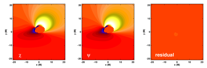
Figure 2: The rotation element $\sin 2\chi$ relating the Stokes parameters measured at the camera to those locally measured relative to lie in the plane of the disc. The left panel shows this quantity calculated by parallel propagation of the camera back to the disc (Shcherbakov & Huang, 2011, and §2.2) while the right panel is calculated by parallel transporting the local polarisation vector to the camera (Connors, Stark & Piran, 1980; Agol, 1997). There is generally good agreement between the two methods, although with up to $\simeq 10\%$ residuals near the black hole in high spin cases.

The accuracy of the method for the parallel transport of a vector in the Kerr metric can be checked by calculating the Penrose-Walker constant at each point along the ray, compared to the value at the camera. In grtrans, this value remains constant along the ray to machine precision. This result is expected, since the parallel transport in the Kerr metric is done analytically (§2.2).

The transported polarisation basis is compared to the polarisation basis of the emission at each point in the so-called comoving orthonormal frame (Shcherbakov & Huang, 2011), where the fluid four-velocity $u^{\mu}=(-1,0,0,0)$. We can verify that this transformation is done correctly in several ways. First, we can verify that $u^{\mu}=(-1,0,0,0)$ after the transformation is done. This is the case again to machine precision.

More interesting tests of the frame transformation come from comparing the combined redshift doppler shift factor $g$ found from $-1/\hat{k}^{t}$ to that obtained from transforming a generic momentum four-vector to the locally non-rotating frame (Bardeen, Press & Teukolsky, 1972) for a generic four-velocity. The result is in equation 17 in Viergutz (1993), and a comparison to the method used here is shown in the left panel of Fig. 1. We find good agreement at all points along the ray. In the right panel of Fig. 1 we compare the angle between $k^{\mu}$ and $b^{\mu}$ in the orthonormal fluid frame to the covariant method for computing the same angle from Broderick (2004):

$$\cos^{2}\theta_{B}=\frac{(b^{\mu}k_{\mu})^{2}}{b^{\nu}b_{\nu}[k^{\sigma}k_{\sigma}+(k^{\rho}u_{\rho})^{2}]}.$$ (73)

The agreement is excellent, with significant deviations only appearing when $k^{\mu}b_{\mu}$ is very small.

We use the method of Shcherbakov & Huang (2011) to project the local polarisation basis in the fluid on to that of the parallel transported polarisation basis of the observer. Connors, Stark & Piran (1980) and Agol (1997) used a similar method, but instead parallel transported local vectors orthogonal and parallel to an accretion disc in the equatorial plane and $k^{\mu}$ to the distant observer. For our purposes, we want the orthogonal vector, which is given in Boyer-Lindquist coordinates as (Agol, 1997),

$$f^{t}_{\perp} = 0,$$ (74)

$$f^{r}_{\perp} = \frac{\sqrt{\Delta}k^{(\theta)}k^{(r)}}{rN_{f}},$$ (75)

$$f^{\theta}_{\perp} = \frac{1}{rN_{f}}\left[k^{(r)^{2}}+(1+v^{2})k^{(\phi)^{2}}-2vk^{(\phi)}k^{(t)}+\right.$$ (77)

$$\left.vk^{(\theta)^{2}}k^{(\phi)}/k^{(t)}\right],$$

$$f^{\phi}_{\perp} = \frac{rk^{(\theta)}}{\sqrt{A}N_{f}}\left[-(1+v^{2})k^{(\phi)}+vk^{(t)}+\right.$$ (79)

$$\left.vk^{(\phi)^{2}}/k^{(t)}\right],$$

where $k^{(\mu)}$ are the components of $k^{\mu}$ in the locally non-rotating frame (Bardeen, Press & Teukolsky, 1972) and $N_{f}$ is a normalisation chosen so that $f^{\mu}_{\perp}f_{\mu,\perp}=1$. The polarisation angle $\psi$ is then given in terms of $K_{1}$ and $K_{2}$ (equation (2.2)):

$$\tan\psi=\frac{-K_{1}\beta-K_{2}\gamma}{K_{2}\beta-K_{1}\gamma}.$$ (80)

We can directly compare this to the rotation angle $\chi$ from equation 45, as long as we identify $b^{\mu}$, used in grtrans as the polarisation reference vector, with their disc normal vector, $f^{\mu}_{\perp}$ above. A comparison between our angle $\chi$ and their $\psi$ is shown in Figure 2 for polarisation from electron scattering in a thin accretion disc. The agreement is mostly good, although with deviations $\lesssim 10\%$ near the event horizon.

These comparisons verify both sets of methods used for calculating redshift/Doppler factors, and angles between the magnetic field and wave vectors and between the polarisation basis in the fluid frame and that of the observer, accounting for parallel transport along the ray. The residual systematic errors $<10\%$ in these quantities, are comparable to the level of accuracy achieved in other parts of the calculation (e.g. the integration or the transfer coefficients).

3.2 Integration tests

We test the accuracy and precision of the different methods for integrating the polarised radiative transfer equations 2.5 through comparison to idealised, analytic solutions with constant coefficients along a ray. We consider two test problems, one for each limiting regime of the equations. The first problem uses only emission and absorption in Stokes I,Q. The analytic solution is given in equation (149), and a comparison of the analytic solution and that calculated using the LSODA integration method is shown in Figure 3. The agreement is excellent to within single precision.

The second problem is the intensity in Stokes $Q$, $U$, $V$ for pure Faraday rotation and conversion ($\rho_{V}$ and $\rho_{Q}$) with emission in $Q$ and $V$. The analytic solution is purely oscillatory, and is given in equation (152). Again the agreement between analytic and numerical solutions is excellent (Fig. 4). In this case the residuals grow with each oscillation. Still, the absolute errors are so small that the error will be negligible unless the Faraday optical depth is enormous, in which case code convergence and run time will also become poor. This is not a limit of interest here, but the issue and some possible solutions are discussed in Shcherbakov, Penna & McKinney (2012).

Figure 3: Analytic (lines) and numerical grtrans (dots) solutions to the polarised emission and absorption test problem (see §3.2, Appendix C) for the Stokes parameters $I$ and $Q$. Single precision accuracy is maintained over the entire ray.

Figure 4: Analytic (lines) and numerical grtrans (dots) solutions to the intrinsic Faraday rotation and conversion test problem (see §3.2, Appendix C) for the Stokes parameters $Q$, $U$, and $V$. The residuals in this case grow along the ray. However, the absolute error remains small unless a very large number of oscillations are present.

3.3 Test problems

Finally we show examples of full test problems based on calculations in the literature. The first example is of the total intensity and linear polarisation of a relativistic, thin accretion disc (Page & Thorne, 1974) in the equatorial plane. The emission is assumed to be optically thick so that the emergent intensity from each point on the disc is a blackbody at the local photospheric temperature. The emergent polarisation is from electron scattering from a semi-infinite slab (Sobolev, 1963; Chandrasekhar, 1950). Figure 5 shows the resulting total intensity, on a log scale, and polarisation vectors. The parameters are $M=10M_{\odot}$, $\dot{M}=0.1\dot{M}_{Edd}$, and the image is integrated over X-ray energies $0.1-10$ keV. The results are in excellent agreement with Figure 1 of Schnittman & Krolik (2009).

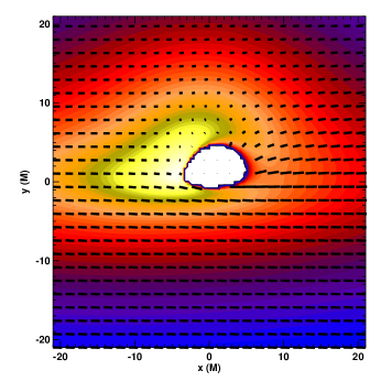
Figure 5: Intensity and linear polarisation map of thermal emission from a thin accretion disc, ignoring the effect of returning radiation (Agol & Krolik, 2000). The intrinsic polarisation is assumed to follow the solution for scattering in a semi-finite atmosphere (Sobolev, 1963; Chandrasekhar, 1950). The black hole mass is $10M_{\odot}$, the accretion rate is $0.1\dot{M}_{\rm edd}$, and the inclination angle is $\theta_{0}=75^{\circ}$. The image is log-scaled with a color scale chosen to match Figure 1 of Schnittman & Krolik (2009). Both the total intensity and polarisation results are in excellent agreement with theirs.

Next we calculate polarised synchrotron radiation from the semi-analytic jet model of Broderick & Loeb (2009). The calculation of the jet structure is described there and in §2.4.4. The electrons in the jet are assumed to follow a power law distribution with a minimum Lorentz factor of $100$. Our transfer coefficients for this case are different than theirs, since we account for the cut off of the distribution function at low energies (see Appendix A). The resulting total intensity and polarisation are shown in Figure 6, and are for the most part in good agreement with those of their M0 model in their Figure 7. The discrepancies are only in the polarisation structure of the counter-jet (bottom right of the image), which could be from differences in how the jet solution is reflected across the plane $z=0$. In any event that region of the image contains little total or polarised flux.

Figure 6: Total intensity (contours) and linear polarisation map from the semi-analytic jet model of Broderick & Loeb (2009). The parameters are $a=0.998$, $\xi=0.5$, $i=25^{\circ}$, $\nu_{0}=345$ GHz. The results are mostly in good agreement with those of their M0 model (Figure 7). The discrepancies arise in the counter-jet, which contains little of the total or polarised flux.

We can also compare the total intensity image from a relativistic MHD simulation between the previous (Dexter, 2011; Dexter et al., 2012) and new versions of the grtrans code (Figure 7). The simulation used the public version of the HARM code (Gammie, McKinney & Tóth, 2003; Noble et al., 2006) with a black hole spin of $a=0.9375$. The simulation results have been scaled to model the submillimetre emission of Sagittarius A*, with a mean electron temperature in the inner disc $\simeq 5\times 10^{10}$ K and an accretion rate chosen so that the flux at $\nu=230$ GHz is roughly $F_{\nu}\simeq 3$ Jy. The agreement between two independent versions of the code is excellent (maximum pixel residuals $\simeq 4\%$ and total flux residual $\simeq 0.3\%$). The previous version used the alternative methods for finding $\theta_{B}$ and $g$ described in §3.1, as well as a quadrature method for the intensity. That code version also interpolated the fluid variables rather than the emission and absorption coefficients. The residuals show that the systematic errors from these different methods lead to only small difference in the resulting total intensity image in a representative case.

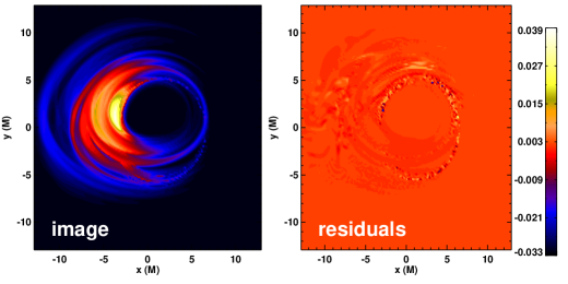
Figure 7: Total intensity false color image of synchrotron radiation from a GRMHD simulation generated with the HARM code from the current version of grtrans, and the residuals between the current and previous versions of the code relative to the maximum overall image intensity. Only one image is shown, since they appear indistinguishable. The two code versions use different methods for handling Doppler beaming, gravitational redshifts, and the integration of the radiative transfer equation. The agreement is excellent between the two cases: the maximum residuals in any pixel are $\sim 4\%$ of the maximum image intensity, and the total flux between the two cases agrees to $\simeq 0.3\%$.

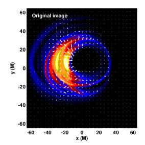
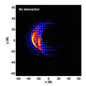
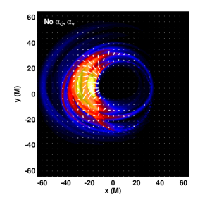
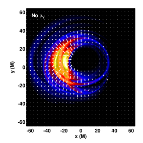
Figure 8: Images and linear polarisation maps of Sgr A* corresponding to the HARM test problem. The top left image includes the full set of absorption and rotation coefficients. In each of the other panels, one or more of these coefficients are ignored to show their different effects on the total intensity and linear polarisation structure. Comparing the top left and bottom right images, for example, shows that intrinsic Faraday rotation is responsible for significantly de-polarising the resulting image. The polarised absorption components play an important role in suppressing the polarisation in the brightest regions of the image. The top right panel shows that self-absorption plays an important role in both the total intensity and polarisation maps.

As a final example, we show images and polarisation maps from the HARM fluid model in Figure 8 with parameters chosen to model the submm bump in Sgr A* (e.g., Mościbrodzka et al., 2009; Dexter et al., 2010). The top left panel includes all absorption and transfer effects. Including the Faraday effects in particular leads to significant rotation of the polarisation vectors and de-polarisation, in contrast to some previous results finding coherent polarisation structures (e.g., Bromley, Melia & Liu, 2001; Broderick & Loeb, 2006) when Faraday effects were ignored. The Faraday effects arise within the emission region itself, even though the electrons are mildly relativistic ($\theta_{e}\sim 10$).

We can understand this result in terms of known expressions for the transfer coefficients (Appendix B). The typical ratio $\nu/\nu_{c}$ for these types of Sgr A* models in the submm is:

$$\frac{\nu}{\nu_{c}}\simeq 40\left(\frac{B}{30\rm G}\right)^{-1}\left(\frac{\theta_{e}}{10}\right)^{-2}\left(\frac{\nu}{230\rm GHz}\right).$$ (81)

At this value, for moderately relativistic temperatures the Faraday coefficients can be much larger than the total absorption coefficient (Figure 12). Jones & Hardee (1979) argued that because this is only true when $\nu/\nu_{c}\gg 1$ where absorption is typically negligible, Faraday rotation and conversion would be negligible in thermal plasmas. However, the submm bump in Sgr A* is likely still marginally self-absorbed (e.g., Falcke et al., 1998; Bower et al., 2015). This is certainly the case for these model images, where the image is significantly modified in the top right panel when absorption is neglected. In these models, the effective optical depth from Faraday effects $\tau=\rho_{\rm Q,V}R\lesssim 100$ and therefore significantly modifies the polarisation structure. Since Faraday effects are sensitive to $\nu/\nu_{c}$ and $\theta_{e}$, the measured coherence of the spatially resolved polarisation structure (e.g., Johnson et al., 2015) provides constraints on these quantities and in turn on the properties of the emitting plasma.

The polarised absorption coefficients also play a role in limiting the polarisation fraction of the brightest pixels of the image (comparing the top left and bottom left panels), but including these components does not have a significant impact on the total intensity image. Images of Sgr A* from previous calculations using only total intensity radiative transfer are then unlikely to be subject to systematic errors from neglecting these coefficients.

4 Code structure and performance

In this section we describe the accuracy, convergence, performance, and scaling of grtrans, and then provide a brief overview of its organisation.

4.1 Convergence

The accuracy of grtrans is very high for smooth solutions (e.g., §3.2), where the coefficients are tabulated over much shorter sections of the ray than the intensity changes appreciably. However, in problems of interest for ray tracing, the emission and absorption coefficients generally change rapidly along the ray, especially in the case of synchrotron radiation where they are strong functions of the fluid state variables. In these cases the rays will generally be sampled sparsely compared to the scale over which the coefficients change. Then the accuracy scales roughly linearly with the number of points along each geodesic, and a sufficient number of points must be chosen to reach the desired accuracy.

Figure 9 shows the convergence of the total flux in the solutions to the HARM and semi-analytic jet problems as a function of $n$, compared to the solution with $n=25600$. For typical problems of interest, the precision is better than $\sim 1\%(n/400)$. The precision is also usually better for the numerical integration method than the formal solution method, although there are cases where the reverse is true (bottom panel Figure 9). In most applications, $n>=400$ should ensure that systematic errors elsewhere in the code (e.g., in the approximations to the synchrotron emissivities) would dominate the total error budget. There is no sign of systematic disagreement between the two integration methods. With $n=25600$, their total fluxes agree to $0.01\%$, consistent with the linear convergence of each method.

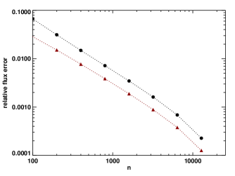
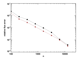
Figure 9: Convergence of the total image flux as a function of the number of points tabulated along each geodesic for the M87 semi-analytic jet (left) and HARM Sgr A* (right) test problems with full polarisation using numerical (black circles) or quadrature (red triangles, equation 54) integration methods. The convergence is roughly linear with $n$, $\Delta F/F\sim 10^{-2}(n/400)$, where the normalization of the error varies at order unity between different problems of interest, camera sizes, and integration methods.

4.2 Performance and scaling

The calculation of the intensity at each camera pixel in ray tracing are independent, and as such it is possible to speed up calculations considerably on multi-core machines by assigning different parts of the calculation to different cores. This is achieved simply in grtrans by using different OpenMP threads for different sets of camera pixels. Although there is overhead associated with creating and destroying threads, the efficiency is still high ($>80\%$ in all problems and on all systems studied), and with the added benefit that memory can be shared by all threads, an important benefit for e.g. the post-processing of high resolution 3D MHD simulations. Alternatively, threads could be used at the level of different images, which might improve the efficiency, but would then provide no speed up for calculating single images.

Figure 10 shows a strong scaling test for grtrans using the spherical accretion example problem. The wall time taken by the parallel part of the code is measured as a function of the number of OpenMP threads on a 24-core workstation. The points are the measured times from single instances of running the code, while the solid line is perfect scaling relative to the measured run time using a single core. The efficiency for this problem peaks at 48 threads (2 threads / core or 1 thread / hyperthread), and is $80-100\%$ for different values of $n$. These results are typical for a wide range of test problems.

4.3 Code organisation

The calculation of radiative transfer around a spinning black hole consists of several independent pieces. In order to maintain flexibility, each of these aspects of the calculation is implemented as a separate Fortran 90 module in grtrans. This Section describes the different modules and how they are used together to run grtrans. More detailed information about the code, explicit examples of its use, and guidelines for adding new fluid and emission models are included in the code distribution.

4.3.1 Kerr null geodesic calculation

Rays in grtrans are assumed to be null geodesics in a Kerr spacetime, and their trajectories in Boyer-Lindquist coordinates are calculated using the semi-analytic public code geokerr (Dexter & Agol, 2009). In addition to the existing public Fortran interfaces for geokerr, there is now also a public Python interface to geokerr compiled using f2py.

The version of geokerr used by grtrans includes a few minor bug fixes from the release version. The most important bug fix is that the option to use $\mu=\cos\theta$ as an independent variable now works robustly even when many turning points are present in a short segment of the orbit. A bug associated with failures in the $\phi$ and $t$ coordinates in rare cases where a ray is sampled extremely close to a turning point has also been fixed.

4.3.2 Fluid models

grtrans is designed to work with a range of models describing the state variables of gas in the Kerr spacetime, from non-relativistic semi-analytic solutions to the fluid equations (e.g., Yuan, Quataert & Narayan, 2003; Broderick et al., 2009; Broderick & Loeb, 2009) to numerical solutions specified on a tabulated grid. These fluid models are implemented separately, one per file, each of which contains a common set of routines to initialise the model (including allocating data), calculate fluid state variables at Boyer-Lindquist coordinate positions in the Kerr metric, and delete the model (including deallocating data). The code currently has several such models implemented as are used in the example problems here. It is straightforward to add new fluid models for use with the code using these existing models as templates.

Since the fluid models are implemented separately, they can be used independently of grtrans. This is useful for testing that the implementation is correct. Examples in the code are included also for using f2py to build Python interfaces to such models, so that their results can be accessed from Python.

4.3.3 Transfer coefficients

In general, the calculation of the transfer coefficients is handled independently of the fluid model. The emission models included at present are synchrotron emission from thermal or power-law particle distributions and optically thick color-corrected blackbody radiation, which can also include linear polarisation induced from electron scattering in a semi-infinite atmosphere.

As with fluid models, the user can include new emission models by using the existing ones as templates. It is also straightforward to combine various emissivities by writing a new one which then calls combinations of those already in use. Examples of this included in the code are the HYBRID and MAXJUTT emissivities, which are combinations of synchrotron emission from thermal+PL and multiple thermal with different temperatures (see Mao et al. 2015 for details).

The synchrotron emissivities can be compiled with f2py and used directly from Python.

4.3.4 Other modules

Many routines associated with the Kerr metric, including the implementation of the method for parallel transport of vectors along geodesics, are stored in their own module. The integration methods for the radiative transfer equation are as well, and also include an f2py interface for use in python.

4.3.5 grtrans driver routine

The main driver routine calculates the intensity at a specified number of observed frequencies and values of other parameters (e.g. mass accretion rate) for a given set of inputs.

The driver routine has global objects associated with the above geodesic, fluid, emissivity, and radiative transfer modules. These are used to store inputs and data. The objects are global so that they can be accessed from the LSODA integration routines.

4.3.6 Python interface

A python class for grtrans includes all of the code inputs and methods for reading the output. There are two main interfaces to the code, either through the use of Fortran input files (namelists) or through the Python wrapper to the code, which compiles with f2py. Both interfaces can be used with Python, while the code can also be run from the command line using input files.

Figure 10: Strong scaling test of the grtrans code using the spherical accretion test problem. The wall time for single runs of the code with $n=500$ (open dots), $1600$ (solid dots) is plotted vs. the number of threads used on a 24-core machine (2 12 core processors). The lines show 100% scaling for the machine based on the execution time for a single thread. The peak efficiency of $\simeq 80-100\%$ for this problem is reached using 2 threads / core. The efficiency exceeds $100\%$ for 48 threads in the $n=1600$ case, either due to run to run variability or improved performance when hyperthreading is in use. The performance range found here also applies to all other problems tested so far, and does not seem to depend on the total number of cores or processors used.

5 Discussion

We have developed a new public code, grtrans, for polarised ray tracing radiative transfer calculations in the Kerr metric, designed with applications to modeling the emission from low-luminosity black holes in mind. For this reason the code is currently focused on synchrotron radiation (Appendix A), and is written to work with a wide range of underlying models for the accreting or outflowing gas, from semi-analytic models (e.g., spherical accretion or force-free jets) to relativistic MHD simulations (e.g., HARM). The code is intended to be modular, so that it is straightforward to add new fluid or emission models. It is written in Fortran to make use of previous work on null geodesics and other routines, but can be used efficiently from Python. We have quantiatively compared results for independent methods for parallel transport and integrating the polarised radiative transfer equations in an effort to verify the code, and presented full examples of comparisons with published work.

The code is written to do ray tracing in the Kerr metric, and as such has two major limitations. First, many aspects of the code assume that the background spacetime is the Kerr metric (e.g. the null geodesic calculation in geokerr and the parallel transport method). Generalising to other spacetimes is possible but would require major changes to the code. The public Gyoto code (Vincent et al., 2011) would probably be a better option for ray tracing in a wide range of spacetimes, although at the moment it does not include polarised radiative transfer. Second, ray tracing assumes that the photon trajectories are known a priori, and so is impractical for calculations where Compton scattering is important but where the total Compton optical depth is small. In this case, one could approximate the scattering locally, or do a first calculation to estimate the effective emission/absorption from scattering. Still, Monte Carlo methods such as those used in grmonty (Dolence et al., 2009) or Pandurata (Schnittman & Krolik, 2013) may be better suited to such problems.

Appendix A Polarised Synchrotron Emission and Absorption Coefficients for Thermal and Power Law Particle Distributions

The subject of radiation from gyrating electrons in a magnetic field has been extensively studied, especially in the relativistic “synchrotron” limit where the electron energy $\gamma\gtrsim 1$ (Westfold, 1959; Ginzburg & Syrovatskii, 1965, 1969; Legg & Westfold, 1968; Sazonov, 1969; Blumenthal & Gould, 1970; Melrose, 1971; Jones & Odell, 1977; Rybicki & Lightman, 1979). However, a consistent treatment of the derivation of the polarised emission and absorption coefficients for the two most commonly used particle distributions (thermal and power law) is still lacking. This appendix gives examples of deriving the various coefficients from integrating the single particle polarised synchrotron emissivity over distributions of particles and provides approximate formulae for their evaluation. The results are compared to emissivities found in the literature and in some cases to numerical integration.

The Stokes basis in the emitting frame has $\mathbf{B}=(0,0,1)$, $\mathbf{e^{1}}=(-\cos{\theta_{B}},0,\sin{\theta_{B}})$ and $\mathbf{e^{2}}=(0,1,0)$ where $\theta_{B}$ is the angle between $B$ and the wave-vector $k$ and $\mathbf{e^{1}}$, $\mathbf{e^{2}}$ are aligned with Stokes $Q$ and $U$ and the projection of $B$ onto the Stokes basis is entirely along $\mathbf{e^{2}}$. Then the vacuum emissivity can be written as a rank-2 tensor (e.g. Melrose, 1980):

$$\eta^{\alpha\beta}=\frac{\sqrt{3}e^{2}}{8\pi c}\nu_{B}\sin{\theta_{B}}H^{\alpha\beta}(\nu,\theta_{B}),$$ (82)

where $e$ is the electron charge, $c$ is the speed of light, $\nu_{B}=\frac{eB}{2\pi mc}$, and

$$H^{11} = F\left(\frac{\nu}{\nu_{c}}\right)-G\left(\frac{\nu}{\nu_{c}}\right),$$ (83)

$$H^{22} = F\left(\frac{\nu}{\nu_{c}}\right)+G\left(\frac{\nu}{\nu_{c}}\right),$$ (84)

$$H^{12} = -H^{21}=\frac{4i\cot{\theta_{B}}}{3\gamma}H\left(\frac{\nu}{\nu_{c}}\right),$$ (85)

where $\nu$ is the emitted frequency, $\gamma$ is the electron Lorentz factor, $\nu_{c}=3/2\nu_{B}\sin{\theta_{B}}\gamma^{2}$ and

$$F(x) = x\int_{x}^{\infty}dyK_{5/3}(y),$$ (86)

$$G(x) = xK_{2/3}(x),$$ (87)

$$H(x) = \int_{x}^{\infty}dyK_{1/3}(y)+xK_{1/3}(x),$$ (88)

are the synchrotron functions for total, linearly and circularly polarised emission respectively and $K_{\alpha}(z)$ is the modified Bessel function.

To compute the emissivity from a distribution of electrons, these formulae are integrated over the particle distribution:

$$j^{\alpha\beta}=\int_{0}^{\infty}d\gamma N(\gamma)\eta^{\alpha\beta}.$$ (89)

The Stokes emissivities are then given as $j_{I}=j^{22}+j^{11}$, $j_{Q}=j^{22}-j^{11}$, $j_{U}=j_{12}+j_{12}$, and $j_{V}=i(j_{12}-j_{21})$. For this Stokes basis, $j_{U}$ vanishes.

The two most commonly used particle distributions for astrophysical sources are the relativistic thermal (Maxwell) distribution,

$$N(\gamma)=\frac{n\gamma^{2}\beta\exp{(-\gamma/\theta_{e})}}{\theta_{e}K_{2}(1/\theta_{e})}$$ (90)

where $n$ is the electron number density and $\theta_{e}=\frac{kT}{mc^{2}}$ is the dimensionless electron temperature; and the power law distribution,

$$N(\gamma)=\left\{\begin{array}[]{lr}n(p-1)(\gamma_{1}^{1-p}-\gamma_{2}^{1-p})^{-1}\gamma^{-p}&\gamma_{1}<\gamma<\gamma_{2}\\ 0&\mathrm{otherwise}\end{array}\right.$$

where $\gamma_{1,2}$ are the low- and high-energy cutoffs of the distribution.

We consider these two cases in turn and derive approximate formulae for their evaluation.

A.1 Ultrarelativistic Thermal Distribution

For the thermal distribution, substituting equation (90) into equation (89) with $\beta\simeq 1$ and $\theta_{e}\gg 1$ gives,

$$j^{\alpha\beta}=\frac{\sqrt{3}ne^{2}\nu_{B}\sin{\theta_{B}}}{8\pi\theta_{e}(2\theta_{e}^{2})}\int_{0}^{\infty}d\gamma\gamma^{2}\exp{(-\gamma/\theta_{e})}H^{\alpha\beta}(\nu,\theta_{B}),$$ (91)

where the approximate form of the modified bessel function for small argument $K_{2}(z)\rightarrow 2z^{2}$ was used. First substitute $z\equiv\gamma/\theta_{e}$ so that,

$$j^{\alpha\beta}=\frac{\sqrt{3}ne^{2}\nu_{B}\sin{\theta_{B}}\theta_{e}^{2}}{8\pi c(2\theta_{e}^{2})}\int_{0}^{\infty}dzz^{2}\exp{(-z)}H^{\alpha\beta}(\nu,\theta_{B}).$$ (92)

Then substitute $\gamma$ for $z$ in the synchrotron functions and use the relations between $j^{\alpha\beta}$ and $j_{I,Q,V}$ to find:

$$j_{I}(\nu,\theta_{B}) = \frac{ne^{2}\nu}{2\sqrt{3}c\theta_{e}^{2}}I_{I}(x),$$ (93)

$$j_{Q}(\nu,\theta_{B}) = \frac{ne^{2}\nu}{2\sqrt{3}c\theta_{e}^{2}}I_{Q}(x),$$ (94)

$$j_{V}(\nu,\theta_{B}) = \frac{2ne^{2}\nu\cot{\theta_{B}}}{3\sqrt{3}c\theta_{e}^{3}}I_{V}(x),$$ (95)

where $x\equiv\nu/\nu_{c}$ and here $\theta_{e}$ takes the place of $\gamma$ in the definition of $\nu_{c}$, and the thermal synchrotron integrals are,

$$I_{I}(x) = \frac{1}{x}\int_{0}^{\infty}dzz^{2}\exp{(-z)}F\left(\frac{x}{z^{2}}\right),$$ (96)

$$I_{Q}(x) = \frac{1}{x}\int_{0}^{\infty}dzz^{2}\exp{(-z)}G\left(\frac{x}{z^{2}}\right),$$ (97)

$$I_{V}(x) = \frac{1}{x}\int_{0}^{\infty}dzz\exp{(-z)}H\left(\frac{x}{z^{2}}\right).$$ (98)

where the function $I_{I}(x)$ corresponds to $I(x_{M})$ from Mahadevan, Narayan & Yi (1996). This result agrees with the formulae from previous work (Sazonov, 1969; Mahadevan, Narayan & Yi, 1996; Huang et al., 2009). The integrals can be approximated analytically with high accuracy by matching the asymptotic behavior for small and large arguments and fitting polynomials in the transition region (Mahadevan, Narayan & Yi, 1996). We find the following approximate forms,

$$I_{I}(x) = 2.5651(1+1.92x^{-1/3}+0.9977x^{-2/3})\exp{(-1.8899x^{1/3})},$$ (99)

$$I_{Q}(x) = 2.5651(1+0.932x^{-1/3}+0.4998x^{-2/3})\exp{(-1.8899x^{1/3})},$$ (100)

$$I_{V}(x) = (1.8138x^{-1}+3.423x^{-2/3}+0.02955x^{-1/2}+2.0377x^{-1/3})\exp{(-1.8899x^{1/3})},$$ (101)

all agree with numerical integration within $\lesssim 1\%$ for all $x$. We further compare the results to numerical integration of the full emissivities using the public symphony code (Pandya et al. 2016). All fitting functions are accurate to within $\lesssim 20\%$ for parameters of interest ($\theta_{e}>3$, $\nu/\nu_{c}>1$), but our circular polarization emissivity has larger deviations at low temperature ($\theta_{e}<1$).

The absorption coefficients are computed from the emission coefficients assuming local thermodynamic equilibrium so that Kirchoff’s Law, $j_{\nu}=\alpha_{\nu}B_{\nu}$, holds with $B_{\nu}$ the blackbody function (e.g. Rybicki & Lightman, 1979).

A.2 Power Law Distribution

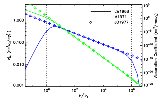
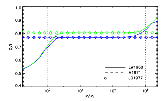
Figure 11: Left: total emission (blue) and absorption (green) coefficients from this work and Legg & Westfold (solid), Melrose (dashed) and Jones & Odell (diamonds). Right: Linear polarisation fraction in emission (blue) and absorption (green) coefficients from this work and Legg & Westfold (solid), Melrose (dashed) and Jones & Odell (diamonds). Here, $\nu_{c}\equiv\nu_{p}\gamma_{1}^{2}$ and the dotted lines show the locations of $\nu/\nu_{c}=1$, $\gamma_{2}^{2}/\gamma_{1}^{2}$, where the approximate forms of the coefficients lose accuracy.

In this case, after plugging in the distribution we change the variable of integration to $x\equiv\nu/\nu_{c}$:

$$j^{\alpha\beta}=\frac{(p-1)ne^{2}\nu_{p}}{4\sqrt{3}c(\gamma_{1}^{1-p}-\gamma_{2}^{1-p})}\left(\frac{\nu}{\nu_{p}}\right)^{-\frac{p-1}{2}}\int_{x_{1}}^{x_{2}}dxx^{\frac{p-3}{2}}H^{\alpha\beta}(\nu,\theta_{B}),$$ (102)

where $\nu_{p}=\nu_{c}/\gamma^{2}$. Then the three emissivities can be written:

$$j_{I} = \frac{ne^{2}(p-1)\nu_{p}}{2\sqrt{3}c(\gamma_{1}^{1-p}-\gamma_{2}^{1-p})}\left(\frac{\nu}{\nu_{p}}\right)^{-\frac{p-1}{2}}[G_{I}(x_{1})-G_{I}(x_{2})],$$ (103)

$$j_{Q} = \frac{ne^{2}(p-1)\nu_{p}}{2\sqrt{3}c(\gamma_{1}^{1-p}-\gamma_{2}^{1-p})}\left(\frac{\nu}{\nu_{p}}\right)^{-\frac{p-1}{2}}[G_{Q}(x_{1})-G_{Q}(x_{2})],$$ (104)

$$j_{V} = \frac{2ne^{2}(p-1)\nu_{p}\cot{\theta_{B}}}{3\sqrt{3}c(\gamma_{1}^{1-p}-\gamma_{2}^{1-p})}\left(\frac{\nu}{\nu_{p}}\right)^{-\frac{p}{2}}[G_{V}(x_{1})-G_{V}(x_{2})],$$ (105)

where the power law synchrotron integrals are,

$$G_{I}(x) = \int_{x}^{\infty}dzz^{\frac{p-3}{2}}F(z),$$ (107)

$$G_{Q}(x) = \int_{x}^{\infty}dzz^{\frac{p-3}{2}}G(z),$$ (108)

$$G_{V}(x) = \int_{x}^{\infty}dzz^{\frac{p}{2}-1}H(z).$$ (109)

In many prior studies (Legg & Westfold, 1968; Blumenthal & Gould, 1970; Melrose, 1971; Jones & Odell, 1977) the integrals are performed analytically for the frequency range $\gamma_{1}^{2}\nu_{p}\ll\nu\ll\gamma_{2}^{2}\nu_{p}$ where the limits of integration, $x_{1,2}=\nu/(\gamma_{1,2}^{2}\nu_{p})$ can be extended to $0$ and $\infty$.

For the primary non-thermal source of interest, M87,

$$\gamma_{1}^{2}\nu_{p}\sim 2\times 10^{11}\left(\frac{B}{10G}\right)\left(\frac{\gamma_{1}}{100}\right)^{2}\text{Hz},$$ (110)

uncomfortably close to frequencies $\simeq 230$ GHz of interest for mm-VLBI (Doeleman et al., 2012; Akiyama et al., 2015) for $\gamma_{1}\gtrsim 30$. We then keep the finite limits of integration and numerically tabulate the integrals $G_{I}$, $G_{Q}$ and $G_{V}$ as functions of $x$ for select values of $p=3.0,3.5,7.0$ currently. This procedure can be sped up significantly using the relation (Westfold, 1959),

$$L(x;s,\alpha) \equiv \int_{x}^{\infty}d\xi\xi^{s-1}\int_{\xi}^{\infty}dyK_{\alpha}(y)$$ (111)

$$= \frac{\alpha+s}{s}\int_{x}^{\infty}d\xi\xi^{s-1}K_{\alpha}(\xi)-\frac{x^{s}}{s}\left[\int_{x}^{\infty}dyK_{\alpha+1}(y)-K_{\alpha}(x)\right]$$

to reduce the double integrals to single integrals. The results agree with those in Legg & Westfold equation (33) after using a recurrence relation,

$$2K_{\alpha}^{\prime}(x)=-(K_{\alpha+1}+K_{\alpha-1}),$$ (112)

and noting that $K_{-\alpha}(x)=K_{\alpha}(x)$ to transform the Bessel functions in $H(x)$.

To check against approximate formulae elsewhere, we extend the limits of integration to $0$ and $\infty$ and use,

$$I(s,\alpha) \equiv \int_{0}^{\infty}dxx^{s}K_{\alpha}(x)=2^{s-1}\Gamma\left(\frac{s+\alpha+1}{2}\right)\Gamma\left(\frac{s-\alpha+1}{2}\right)$$ (113)

$$J(s,\alpha) \equiv L(0;s+1,\alpha-1)=\frac{\alpha+s}{s+1}I(s,\alpha-1)$$ (114)

$$= \frac{\alpha+s}{s+1}2^{s-1}\Gamma\left(\frac{s+\alpha}{2}\right)\Gamma\left(\frac{s-\alpha}{2}+1\right)$$

to find the approximate forms $G_{I,Q,V}(0)-G_{I,Q,V}(\infty)$:

$$G_{I}(0) = J\left(\frac{p-1}{2},\frac{5}{3}\right)=\frac{2^{\frac{p-3}{2}}(p+7/3)}{p+1}\Gamma\left(\frac{p}{4}+\frac{7}{12}\right)\Gamma\left(\frac{p}{4}-\frac{1}{12}\right),$$ (115)

$$G_{Q}(0) = I\left(\frac{p-1}{2},\frac{2}{3}\right)=\frac{p+1}{p+7/3}G_{I}(0),$$ (116)

$$G_{V}(0) = J\left(\frac{p}{2}-1,\frac{1}{3}\right)+I\left(\frac{p}{2},\frac{1}{3}\right)$$ (117)

$$= \frac{2^{\frac{p}{2}-1}(p+2)}{p}\Gamma\left(\frac{p}{4}+\frac{1}{3}\right)\Gamma\left(\frac{p}{4}+\frac{2}{3}\right),$$

$$G_{I,Q,V}(\infty) = 0$$ (118)

leading to the approximate emissivities:

$$j_{I}^{0} = \frac{ne^{2}(p-1)\nu_{p}}{2\sqrt{3}c(\gamma_{1}^{1-p}-\gamma_{2}^{1-p})}\left(\frac{\nu}{\nu_{p}}\right)^{-\frac{p-1}{2}}2^{\frac{p-3}{2}}\frac{p+7/3}{p+1}\Gamma\left(\frac{p}{4}+\frac{7}{12}\right)\Gamma\left(\frac{p}{4}-\frac{1}{12}\right),$$ (119)

$$j_{Q}^{0} = \frac{p+1}{p+7/3}j_{I}^{0},$$ (120)

$$j_{V}^{0} = \frac{2ne^{2}(p-1)\nu_{p}\cot{\theta_{B}}}{3\sqrt{3}c(\gamma_{1}^{1-p}-\gamma_{2}^{1-p})}\left(\frac{\nu}{\nu_{p}}\right)^{-\frac{p}{2}}2^{\frac{p}{2}-1}\frac{p+2}{p}\Gamma\left(\frac{p}{4}+\frac{1}{3}\right)\Gamma\left(\frac{p}{4}+\frac{2}{3}\right).$$ (121)

These results agree with those of several authors.

In the case of non-thermal emission, the absorption coefficient cannot be simply related to the emissivity using Kirchoff’s Law, and instead we use (Melrose, 1980):

$$\alpha^{\alpha\beta}=-\frac{c}{m\nu^{2}}\int_{0}^{\infty}d\gamma\gamma^{2}\frac{d}{d\gamma}\left[\frac{N(\gamma)}{\gamma^{2}}\right]\eta^{\alpha\beta}(\gamma,\nu,\theta_{B}).$$ (122)

The derivation is analogous to that for the emissivity, and the results are:

$$\alpha_{I} = \frac{ne^{2}(p-1)(p+2)}{4\sqrt{3}mc\nu_{p}(\gamma_{1}^{1-p}-\gamma_{2}^{1-p})}\left(\frac{\nu}{\nu_{p}}\right)^{-\frac{p}{2}-2}\left[Ga_{I}(x_{1})-Ga_{I}(x_{2})\right],$$ (123)

$$\alpha_{Q} = \frac{ne^{2}(p-1)(p+2)}{4\sqrt{3}mc\nu_{p}(\gamma_{1}^{1-p}-\gamma_{2}^{1-p})}\left(\frac{\nu}{\nu_{p}}\right)^{-\frac{p}{2}-2}\left[Ga_{Q}(x_{1})-Ga_{Q}(x_{2})\right],$$ (124)

$$\alpha_{V} = \frac{ne^{2}(p-1)(p+2)\cot{\theta_{B}}}{3\sqrt{3}mc\nu_{p}(\gamma_{1}^{1-p}-\gamma_{2}^{1-p})}\left(\frac{\nu}{\nu_{p}}\right)^{-\frac{p+5}{2}}\left[Ga_{V}(x_{1})-Ga_{V}(x_{2})\right]$$ (125)

where the power law absorption integrals are,

$$Ga_{I}(x) = \int_{x}^{\infty}dzz^{\frac{p}{2}-1}F(z),$$ (126)

$$Ga_{Q}(x) = \int_{x}^{\infty}dzz^{\frac{p}{2}-1}G(z),$$ (127)

$$Ga_{V}(x) = \int_{x}^{\infty}dzz^{\frac{p-1}{2}}H(z).$$ (128)

Again extending the limits of integration, we find agreement with approximate formulae in the literature:

$$Ga_{I}(0) = \frac{p+10/3}{p+1}2^{\frac{p}{2}-1}\Gamma\left(\frac{p}{4}+\frac{5}{6}\right)\Gamma\left(\frac{p}{4}+\frac{1}{6}\right),$$ (129)

$$Ga_{Q}(0) = \frac{p+2}{p+10/3}Ga_{I}(0)$$ (130)

$$Ga_{V}(0) = \frac{p+3}{p+1}2^{\frac{p-1}{2}}\Gamma\left(\frac{p}{4}+\frac{7}{12}\right)\Gamma\left(\frac{p}{4}+\frac{11}{12}\right),$$ (131)

$$Ga_{I,Q,V}(\infty) = 0.$$ (132)

Figure 11 compares numerical integration of the formulae in Equations (103) and (123) with the forms from the literature.

Appendix B Faraday coefficients for power law and thermal distributions of electrons

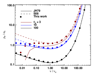
Figure 12: Left: Ratio of thermal Faraday conversion coefficient to total absorption as a function of $\nu/\nu_{c}$ at $\theta_{e}=100$ calculated from numerical integration of the expression in Jones & Hardee (1979) (solid line, equation (141)), the fitting function approach introduced by Shcherbakov (2008) (dashed line, equation (136)), and in this work (black dots, equation (145)). Right: Same as the left panel but for Faraday rotation at 3 different temperatures. In both cases all results agree at high frequencies and temperatures. Our fitting functions use the temperature dependence from Shcherbakov (2008) along with the low-frequency limits from Jones & Hardee (1979).

As well as the emission and absorption coefficients calculated above (Appendix A), the coefficients $\rho_{V}$ and $\rho_{Q}$ affect the generation and transfer of polarisation in a magnetised plasma. We use approximate expressions from the literature for these coefficients which as above are modified to i) be fast to evaluate and ii) have the correct asymptotic limits.

B.1 Power law distribution

In the case of a power law distribution, we use the expressions from Jones & Odell (1977) Appendix C, written in our notation:

$$\rho_{Q} = -\rho_{\perp}\left(\frac{\nu_{B}}{\nu}\right)^{3}\gamma_{\rm min}^{2-p}\left[\left(1-\left(\frac{\nu_{\rm min}}{\nu}\right)^{p/2-1}\right)\left(p/2-1\right)^{-1}\right],$$ (133)

$$\rho_{V} = 2\frac{p+2}{p+1}\rho_{\perp}\left(\frac{\nu_{B}}{\nu}\right)^{2}\gamma_{\rm min}^{-(p+1)}\ln\gamma_{\rm min}\cot{\theta_{B}},$$ (134)

$$\rho_{\perp} = \frac{ne^{2}}{mc\nu_{B}}(p-1)\left[\gamma_{\rm min}^{1-p}-\gamma_{\rm max}^{1-p}\right]^{-1}.$$ (135)

More accurate expressions (Huang & Shcherbakov, 2011) require integration over the distribution function and for this reason are slow to evaluate. These approximate forms are relatively accurate for $\gamma_{\rm min}\lesssim 10^{2}$ (left panel of Fig. 6 in Huang & Shcherbakov, 2011). In the example semi-analytic jet problem above, Faraday rotation and conversion are negligible (Broderick & Loeb, 2009). Nonetheless, it should be possible to find accurate fitting functions for these coefficients, which would be consistent with our approach for the other coefficients.

B.2 Thermal distribution

Faraday coefficients for thermal distributions of electrons have been calculated in limits of either high frequency $\nu/\nu_{c}\gg 1$ (e.g., Melrose, 1997), at high temperatures $\theta_{e}\gg 1$, or both. In particular, Shcherbakov (2008) provided approximate fitting functions for $\rho_{V}$ and $\rho_{Q}$ over a wide temperature range $\theta_{e}\gtrsim 1$ with high accuracy for $\nu/\nu_{c}\gtrsim 10^{-1}$ (their equations 25, 26, 33, but in our notation):

$$\rho_{Q} = \frac{ne^{2}\nu_{B}^{2}\sin{\theta_{B}}^{2}}{mc\nu^{3}}f(X)\left[\frac{K_{1}(\theta_{e}^{-1})}{K_{2}(\theta_{e}^{-1})}+6\theta_{e}\right]$$ (136)

$$\rho_{V} = \frac{2ne^{2}\nu_{B}}{mc\nu^{2}}\frac{K_{0}(\theta_{e}^{-1})}{K_{2}(\theta_{e}^{-1})}\cos{\theta_{B}}g(X),$$ (137)

where

$$f(X) = 2.011\exp\left(-\frac{X^{1.035}}{4.7}\right)-\cos\left(\frac{X}{2}\right)\exp\left(-\frac{X^{1/2}}{2.73}\right)-0.011\exp\left(-\frac{X}{47.2}\right)$$ (138)

$$g(X) = 1-0.11\ln\left(1+0.035X\right)$$ (139)

$$X = \left(\frac{3}{2\sqrt{2}}10^{-3}\frac{\nu}{\nu_{c}}\right)^{-1/2},$$ (140)

and their parameter $X$ is a function of $\nu/\nu_{c}$. In the high-frequency limit $\nu/\nu_{c}\gg 1$, both functions asymptotically reach unity. The cosine term in $f(X)$ is used to fit the sign change in $\rho_{Q}$ near $\nu/\nu_{c}\simeq 1.5$.

While the high frequency and high temperature limit is most relevant for our applications of interest, e.g. modeling the submm emission from Sgr A*, ideally we would have expressions that are correct in both asymptotic limits. For this reason we modify the expressions in Shcherbakov (2008), by comparing them with the expressions for the high temperature synchrotron limit given in Jones & Hardee (1979) (their equations 3-4, in our notation):

$$\rho_{Q} = \frac{\pi ne^{2}(\nu/\nu_{c})^{-2/3}}{2^{4/3}3^{2/3}mc\theta_{e}^{3}\nu}J_{4}(\nu/\nu_{c}),$$ (141)

$$\rho_{V} = \frac{ne^{2}\nu_{B}\cos{\theta_{B}}}{mc\nu^{2}\theta_{e}^{2}}J_{5}(\nu/\nu_{c},\theta_{e},\theta_{B}),$$ (142)

where

$$J_{4}(z) = \int_{0}^{\infty}dyy^{4/3}Gi^{\prime}(q)e^{-y},$$ (143)

$$J_{5}(z,\theta_{e},\theta_{B}) = \int_{0}^{\infty}dy\left[\ln(y\theta_{e})+\sin{\theta_{B}}\ln 2+1/3\left[q\pi Gi(q)-1\right]+1/2\int_{q}^{\infty}dx\left(\pi Gi(x)-1/x\right)\right]e^{-y},$$ (144)

and where $q\equiv(3/2z/y^{2})^{2/3}$ and $Gi(x)$ is defined in terms of Airy functions (Abramowitz & Stegun, 1970).

In the high-frequency, high temperature limit where $\nu/\nu_{c}\gg 1$, $\theta_{e}\gg 1$, and where we can replace the Bessel functions by their asymptotic limits and $J_{4}\rightarrow-24/\pi(3/2z)^{-4/3}$, $J_{5}\rightarrow\ln\theta_{e}$, these expressions agree with the above results from Shcherbakov (2008). From numerically integrating $J_{4}(z)$ and $J_{5}(z)$, we also find good agreement between the two sets of coefficients over their reported ranges of validity. We adapt the fitting function $f(X)$ in Shcherbakov (2008) to use the asymptotic limit of $\rho_{Q}$ at small $\nu/\nu_{c}$, where $J_{4}(z)\rightarrow\frac{4}{9\times 3^{5/6}}$:

$$f_{m}(X)=f(X)+\left[0.011\exp{\left(-\frac{X}{47.2}\right)}-2^{-1/3}/3^{23/6}10^{4}\pi X^{-8/3}\right]1/2\left[1+\tanh{\left(10\ln{x/120}\right)}\right].$$ (145)

The added term imposes the correct asymptotic limit at large $X$ (small $\nu/\nu_{c}$) and for this reason maintains good accuracy over all $\nu/\nu_{c}$.

For $\rho_{V}$, the term $J5(\nu/\nu_{c})$ from Jones & Hardee (1979) separates into a sum of terms which depend on temperature and $\theta_{B}$, and those which only depend on $\nu/\nu_{c}$. This suggests that it would be better to use the factor $g(X)$ in Shcherbakov (2008) as a difference from the high-frequency limit rather than a multiplication:

$$\rho_{V}=\frac{2ne^{2}\nu_{B}\cos{\theta_{B}}}{mc\nu^{2}}\frac{K_{0}(\theta_{e}^{-1})-\Delta J_{5}(X)}{K_{2}(\theta_{e}^{-1})},$$ (146)

where we define our correction factor $\Delta J_{5}(X)$ in a similar spirit to that of Shcherbakov (2008), but modified for higher accuracy:

$$\Delta J_{5}(X)=0.4379\ln(1+0.001858X^{1.503}).$$ (147)

Figure 12 compares numerical integration of equation (141) (Jones & Hardee, 1979) with the fitting functions from equation (136) (Shcherbakov, 2008) and our modified forms. Our approximate versions are fast to compute, while maintaining accuracy over all $\nu/\nu_{c}$.

We have compared polarised spectra and maps from HARM models of Sgr A* computed using the prescriptions from Shcherbakov (2008), Jones & Hardee (1979), and the high temperature, high frequency limit. As expected, all expressions are in excellent agreement when $\nu/\nu_{c}\gg 1$, in this case for $\nu\gtrsim 10^{12}$ Hz. Below that, our modified expressions and those from Shcherbakov (2008) are in good agreement, while the degree of circular polarisation can differ between our results and the high-frequency limit. As described in the main text, models of Sgr A* in the submm have self-absorption optical depth $\tau_{I}\gtrsim 1$, $\nu/\nu_{c}\sim 10-100$, and $\theta_{e}\sim 10$, so that the Faraday optical depths can be very large and have an important effect on the resulting polarisation maps and spectra (e.g. Figure 8). Since this result is for the high-frequency, relativistic limit, it does not depend on the fitting function used.

Appendix C Analytic solutions to the polarised radiative transfer equations

This appendix provides the analytic solutions to the polarised radiative transfer equations used for testing different integration methods for grtrans in §3.2. In all cases, the boundary condition used is that the initial intensity is zero for each Stokes parameter.

The first case considered is pure emission and absorption in stokes $I$ and $Q$, in which case equation (47) becomes:

$$\frac{d}{ds}\left(\begin{array}[]{c}I\\ Q\\ \end{array}\right)=\left(\begin{array}[]{c}j_{I}\\ j_{Q}\\ \end{array}\right)-\left(\begin{array}[]{cc}\alpha_{I}&\alpha_{Q}\\ \alpha_{Q}&\alpha_{I}\\ \end{array}\right)\left(\begin{array}[]{c}I\\ Q\\ \end{array}\right),$$ (148)

whose solution is,

$$I(s) = \frac{1}{\alpha(\alpha_{I}-\alpha_{Q})}\left\{(j_{I}\alpha_{I}-j_{Q}\alpha_{Q})\left[1-\frac{e^{-\alpha s}}{2}(1+e^{2\alpha_{Q}s})\right]+(j_{I}\alpha_{Q}-j_{Q}\alpha_{I})\frac{e^{-\alpha s}}{2}(1-e^{2\alpha_{Q}s})\right\},$$ (149)

$$Q(s) = \frac{1}{\alpha(\alpha_{I}-\alpha_{Q})}\left\{(j_{Q}\alpha_{I}-j_{I}\alpha_{Q})\left[1-\frac{e^{-\alpha s}}{2}\left(1+e^{2\alpha_{Q}s}\right)\right]+(j_{Q}\alpha_{Q}-j_{I}\alpha_{I})\frac{e^{-\alpha s}}{2}\left(1-e^{2\alpha_{Q}s}\right)\right\},$$ (150)

where $\alpha\equiv\alpha_{I}+\alpha_{Q}$. When $\alpha_{Q}=0$, the second group of terms in each equation vanishes while the first reduces to the usual formal solution of the radiative transfer equation, e.g. when stokes $I$ and $Q$ are not coupled. Examples of the solution are shown in Figure 3.

The second case of interest is pure polarised emission in Stokes $(Q,U,V)$ along with Faraday rotation and conversion ($\rho_{Q,V}$). Here the polarised radiative transfer equation is,

$$\frac{d}{ds}\left(\begin{array}[]{c}Q\\ U\\ V\\ \end{array}\right)=\left(\begin{array}[]{c}j_{Q}\\ j_{U}\\ j_{V}\end{array}\right)-\left(\begin{array}[]{cccc}0&\rho_{V}&0\\ -\rho_{V}&0&\rho_{Q}\\ 0&-\rho_{Q}&0\\ \end{array}\right)\left(\begin{array}[]{c}Q\\ U\\ V\\ \end{array}\right),$$ (151)

where we have set $\rho_{U}=0$ as is commonly chosen for the Stokes basis for synchrotron radiation. From this equation it is apparent that $\rho_{V}$ is responsible for changing the linear polarisation direction (mixing stokes $Q$ and $U$, Faraday rotation) while $\rho_{Q}$ converts between linear and circular polarisation (mixing stokes $U$ and $V$, Faraday conversion). The solution is,

$$Q(s) = \frac{\rho_{Q}}{\rho^{2}}(j_{Q}\rho_{Q}+j_{V}\rho_{V})s-\frac{\rho_{V}}{\rho^{3}}(j_{V}\rho_{Q}-j_{Q}\rho_{V})\sin{\rho s}-\frac{j_{U}\rho_{V}}{\rho^{2}}(1-\cos{\rho s})$$ (152)

$$U(s) = \frac{j_{Q}\rho_{V}-j_{V}\rho_{Q}}{\rho^{2}}(1-\cos{\rho s})+\frac{j_{U}}{\rho}\sin{\rho s},$$ (153)

$$V(s) = \frac{\rho_{V}}{\rho^{2}}(j_{Q}\rho_{Q}+j_{V}\rho_{V})s-\frac{\rho_{Q}}{\rho^{3}}(j_{Q}\rho_{V}-j_{V}\rho_{Q})\sin{\rho s}+\frac{j_{U}\rho_{Q}}{\rho^{2}}(1-\cos{\rho s}),$$ (154)

where $\rho\equiv\sqrt{\rho_{Q}^{2}+\rho_{V}^{2}}$. These solutions for a sample case are plotted in Figure 4.

In the case of only Faraday rotation or conversion ($\rho_{Q}=0$ for Stokes $Q$ or $\rho_{V}=0$ for Stokes $V$), the solution is purely oscillatory with the maximum linearly polarised intensity restricted to be $\sim j/\rho$ independent of the total intensity or path length, despite the fact that there is no absorption. Since in this optically thin limit the total intensity grows as $j_{I}s$, the fractional polarisation decreases as $1/s$. When both Faraday rotation and conversion are present, the Stokes $Q$ and $V$ acquire terms which linearly increase with $s$, while the oscillatory terms still have maximum values that are independent of $s$. This means that in the limit of large Faraday optical depth (large $s$), the fractional polarisation approaches a constant value $Q,V/I=\rho_{Q,V}(j_{Q}\rho_{Q}+j_{V}\rho_{V})/j_{I}\rho^{2}$ instead of decreasing as $1/s$ in the pure Faraday rotation or conversion case. Since for cases of interest $\rho_{V}>\rho_{Q}$, circular polarisation becomes dominant over linear polarisation in the limit of large Faraday optical depth.

This is a different limit than an initial polarised intensity travel through a magnetised medium where Faraday rotation occurs. In that case, the intensity also oscillates between Stokes $Q$ and $U$, but with a constant polarised intensity. The fractional polarisation only decreases when the Faraday rotation is instead occurring in the region where the polarised emission is being produced.

Appendix D Closed form expression for $\mathbf{O}(s,s^{\prime})$

Landi Degl’Innocenti & Landi Degl’Innocenti (1985) found a closed form solution for the matrix operator $\mathbf{O}(s,s^{\prime})$, defined by

$$\frac{d}{ds}\mathbf{O}(s,s^{\prime})=-\mathbf{K}(s)\mathbf{O}(s,s^{\prime}),\hskip 12.0pt\mathbf{O}(s,s)=1,$$ (156)

which describes the transfer of the Stokes parameters from position $s$ to $s^{\prime}$ in the absence of emission, which is valid under limited conditions including when the absorption matrix $\mathbf{K}$ is constant over the interval. We reproduce the solution here in our notation:

$$\mathbf{O}(s,s^{\prime})=\exp(-\alpha_{I}\Delta s)\left\{\left[\cosh{\left(\Lambda_{1}\Delta s\right)}+\cos{\left(\Lambda_{2}\Delta s\right)}\right]\mathbf{M_{1}}/2-\sin{\left(\Lambda_{2}\Delta s\right)}\mathbf{M_{2}}-\sinh{\left(\Lambda_{1}\Delta s\right)}\mathbf{M_{3}}+\left[\cosh{\left(\Lambda_{1}\Delta s\right)}-\cos{\left(\Lambda_{2}\Delta s\right)}\right]\mathbf{M_{4}}/2\right\},$$ (157)

where

$$\mathbf{M_{1}} = \mathbf{1}$$ (158)

$$\mathbf{M_{2}} = \frac{1}{\Theta}\left(\begin{array}[]{cccc}0&\Lambda_{2}\alpha_{Q}-\sigma\Lambda_{1}\rho_{Q}&\Lambda_{2}\alpha_{U}-\sigma\Lambda_{1}\rho_{U}&\Lambda_{2}\alpha_{V}-\sigma\Lambda_{1}\rho_{V}\\ \Lambda_{2}\alpha_{Q}-\sigma\Lambda_{1}\rho_{Q}&0&\sigma\Lambda_{1}\alpha_{V}+\Lambda_{2}\rho_{V}&-\sigma\Lambda_{1}\alpha_{U}-\Lambda_{2}\rho_{U}\\ \Lambda_{2}\alpha_{U}-\sigma\Lambda_{1}\rho_{U}&-\sigma\Lambda_{1}\alpha_{V}-\Lambda_{2}\rho_{V}&0&\sigma\Lambda_{1}\alpha_{Q}+\Lambda_{2}\rho_{Q}\\ \Lambda_{2}\alpha_{V}-\sigma\Lambda_{1}\rho_{V}&\sigma\Lambda_{1}\alpha_{U}+\Lambda_{2}\rho_{U}&-\sigma\Lambda_{1}\alpha_{Q}-\Lambda_{2}\rho_{Q}&0\\ \end{array}\right)$$ (163)

$$\mathbf{M_{3}} = \frac{1}{\Theta}\left(\begin{array}[]{cccc}0&\Lambda_{1}\alpha_{Q}+\sigma\Lambda_{2}\rho_{Q}&\Lambda_{1}\alpha_{U}+\sigma\Lambda_{2}\rho_{Q}&\Lambda_{1}\alpha_{V}+\sigma\Lambda_{2}\rho_{V}\\ \Lambda_{1}\alpha_{Q}+\sigma\Lambda_{2}\rho_{Q}&0&-\sigma\Lambda_{2}\alpha_{V}+\Lambda_{1}\rho_{V}&\sigma\Lambda_{2}\alpha_{U}-\Lambda_{1}\rho_{U}\\ \Lambda_{1}\alpha_{U}+\sigma\Lambda_{2}\rho_{U}&\sigma\Lambda_{2}\alpha_{V}-\Lambda_{1}\rho_{V}&0&-\sigma\Lambda_{2}\alpha_{Q}+\Lambda_{1}\rho_{Q}\\ \Lambda_{1}\alpha_{V}+\sigma\Lambda_{2}\rho_{V}&-\sigma\Lambda_{2}\alpha_{U}+\Lambda_{1}\rho_{U}&\sigma\Lambda_{2}\alpha_{Q}-\Lambda_{1}\rho_{Q}&0\\ \end{array}\right)$$ (168)

$$\mathbf{M_{4}} = \frac{2}{\Theta}\left(\begin{array}[]{cccc}\left(\alpha^{2}+\rho^{2}\right)/2&\alpha_{V}\rho_{U}-\alpha_{U}\rho_{V}&\alpha_{Q}\rho_{V}-\alpha_{V}\rho_{Q}&\alpha_{U}\rho_{Q}-\alpha_{Q}\rho_{U}\\ \alpha_{U}\rho_{V}-\alpha_{V}\rho_{U}&\alpha_{Q}^{2}+\rho_{Q}^{2}-\left(\alpha^{2}+\rho^{2}\right)/2&\alpha_{Q}\alpha_{U}+\rho_{Q}\rho_{U}&\alpha_{V}\alpha_{Q}+\rho_{V}\rho_{Q}\\ \alpha_{V}\rho_{Q}-\alpha_{Q}\rho_{V}&\alpha_{Q}\alpha_{U}+\rho_{Q}\rho_{U}&\alpha_{U}^{2}+\rho_{U}^{2}-\left(\alpha^{2}+\rho^{2}\right)/2&\alpha_{U}\alpha_{V}+\rho_{U}\rho_{V}\\ \alpha_{Q}\rho_{U}-\alpha_{U}\rho_{Q}&\alpha_{V}\alpha_{Q}+\rho_{V}\rho_{Q}&\alpha_{U}\alpha_{V}+\rho_{U}\rho_{V}&\alpha_{V}^{2}+\rho_{V}^{2}-\left(\alpha^{2}+\rho^{2}\right)/2\\ \end{array}\right)$$ (173)

and

$$\Theta = 2\left[\left(\alpha^{2}-\rho^{2}\right)^{2}/4+\left(\mathbf{\alpha}\cdot\mathbf{\rho}\right)^{2}\right]^{1/2},$$ (175)

$$\Lambda_{1,2} = \left\{\left[\left(\alpha^{2}-\rho^{2}\right)^{2}/4+\left(\mathbf{\alpha}\cdot\mathbf{\rho}\right)^{2}\right]^{1/2}\pm\left(\alpha^{2}-\rho^{2}\right)/2\right\}^{1/2},$$ (176)

$$\sigma = \rm sign\left(\mathbf{\alpha}\cdot\mathbf{\rho}\right),$$ (177)

$$\mathbf{\alpha}\cdot\mathbf{\rho} = \alpha_{Q}\rho_{Q}+\alpha_{U}\rho_{U}+\alpha_{V}\rho_{V},$$ (178)

$$\rho^{2} = \rho_{Q}^{2}+\rho_{U}^{2}+\rho_{V}^{2},$$ (179)

$$\alpha^{2} = \alpha_{Q}^{2}+\alpha_{U}^{2}+\alpha_{V}^{2}.$$ (180)

References

- Abramowitz & Stegun (1970) Abramowitz M., Stegun I. A., 1970, Handbook of mathematical functions : with formulas, graphs, and mathematical tables
- Agol (1997) Agol E., 1997, PhD thesis, University of California, Santa Barbara
- Agol & Krolik (2000) Agol E., Krolik J. H., 2000, ApJ, 528, 161
- Akiyama et al. (2015) Akiyama K. et al., 2015, ApJ, 807, 150
- Balbus & Hawley (1991) Balbus S. A., Hawley J. F., 1991, ApJ, 376, 214
- Bardeen, Press & Teukolsky (1972) Bardeen J. M., Press W. H., Teukolsky S. A., 1972, ApJ, 178, 347
- Beckwith, Hawley & Krolik (2008) Beckwith K., Hawley J. F., Krolik J. H., 2008, MNRAS, 390, 21
- Blumenthal & Gould (1970) Blumenthal G. R., Gould R. J., 1970, Reviews of Modern Physics, 42, 237
- Bower et al. (2015) Bower G. C. et al., 2015, ApJ, 802, 69
- Broderick & Blandford (2004) Broderick A., Blandford R., 2004, MNRAS, 349, 994
- Broderick (2004) Broderick A. E., 2004, PhD thesis, California Institute of Technology, California, USA
- Broderick et al. (2009) Broderick A. E., Fish V. L., Doeleman S. S., Loeb A., 2009, ApJ, 697, 45
- Broderick & Loeb (2005) Broderick A. E., Loeb A., 2005, MNRAS, 363, 353
- Broderick & Loeb (2006) —, 2006, ApJ, 636, L109
- Broderick & Loeb (2009) —, 2009, ApJ, 697, 1164
- Bromley, Melia & Liu (2001) Bromley B. C., Melia F., Liu S., 2001, ApJ, 555, L83
- Chan et al. (2015) Chan C.-K., Psaltis D., Özel F., Narayan R., Saḑowski A., 2015, ApJ, 799, 1
- Chandrasekhar (1950) Chandrasekhar S., 1950, Radiative transfer. Oxford, Clarendon Press
- Chandrasekhar (1983) —, 1983, The mathematical theory of black holes. Oxford/New York, Clarendon Press/Oxford University Press
- Chen et al. (2015) Chen B., Kantowski R., Dai X., Baron E., Maddumage P., 2015, ApJS, 218, 4
- Connors & Stark (1977) Connors P. A., Stark R. F., 1977, Nature, 269, 128
- Connors, Stark & Piran (1980) Connors P. A., Stark R. F., Piran T., 1980, ApJ, 235, 224
- Cunningham (1975) Cunningham C. T., 1975, ApJ, 202, 788
- Dauser et al. (2010) Dauser T., Wilms J., Reynolds C. S., Brenneman L. W., 2010, MNRAS, 409, 1534
- Davis & Hubeny (2006) Davis S. W., Hubeny I., 2006, ApJS, 164, 530
- De Villiers & Hawley (2003) De Villiers J.-P., Hawley J. F., 2003, ApJ, 589, 458
- Dexter (2011) Dexter J., 2011, PhD thesis, University of Washington
- Dexter & Agol (2009) Dexter J., Agol E., 2009, ApJ, 696, 1616
- Dexter & Agol (2011) —, 2011, ApJ, 727, L24
- Dexter, Agol & Fragile (2009) Dexter J., Agol E., Fragile P. C., 2009, ApJ, 703, L142
- Dexter et al. (2010) Dexter J., Agol E., Fragile P. C., McKinney J. C., 2010, ApJ, 717, 1092
- Dexter et al. (2012) —, 2012, Journal of Physics Conference Series, 372, 012023
- Dexter & Fragile (2011) Dexter J., Fragile P. C., 2011, ApJ, 730, 36
- Dexter, McKinney & Agol (2012) Dexter J., McKinney J. C., Agol E., 2012, MNRAS, 421, 1517
- Dexter & Quataert (2012) Dexter J., Quataert E., 2012, MNRAS, 426, L71
- Doeleman et al. (2009) Doeleman S. et al., 2009, in ArXiv Astrophysics e-prints, Vol. 2010, astro2010: The Astronomy and Astrophysics Decadal Survey, p. 68
- Doeleman et al. (2012) Doeleman S. S. et al., 2012, Science, 338, 355
- Dolence et al. (2009) Dolence J. C., Gammie C. F., Mościbrodzka M., Leung P. K., 2009, ApJS, 184, 387
- Eisenhauer et al. (2008) Eisenhauer F. et al., 2008, in Society of Photo-Optical Instrumentation Engineers (SPIE) Conference Series, Vol. 7013, Society of Photo-Optical Instrumentation Engineers (SPIE) Conference Series, p. 2
- Falcke et al. (1998) Falcke H., Goss W. M., Matsuo H., Teuben P., Zhao J., Zylka R., 1998, ApJ, 499, 731
- Font, Ibáñez & Papadopoulos (1999) Font J. A., Ibáñez J. M., Papadopoulos P., 1999, MNRAS, 305, 920
- Gammie & Leung (2012) Gammie C. F., Leung P. K., 2012, ApJ, 752, 123
- Gammie, McKinney & Tóth (2003) Gammie C. F., McKinney J. C., Tóth G., 2003, ApJ, 589, 444
- Ginzburg & Syrovatskii (1965) Ginzburg V. L., Syrovatskii S. I., 1965, ARA&A, 3, 297
- Ginzburg & Syrovatskii (1969) —, 1969, ARA&A, 7, 375
- Gold et al. (2016) Gold R., McKinney J. C., Johnson M. D., Doeleman S. S., 2016, ArXiv e-prints
- Hindmarsh (1983) Hindmarsh A. C., 1983, in Scientific Computing, R. S. Stepleman et al., ed., pp. 55–64
- Huang et al. (2009) Huang L., Liu S., Shen Z., Yuan Y., Cai M. J., Li H., Fryer C. L., 2009, ApJ, 703, 557
- Huang & Shcherbakov (2011) Huang L., Shcherbakov R. V., 2011, MNRAS, 416, 2574
- Johnson et al. (2015) Johnson M. D. et al., 2015, Science, 350, 1242
- Jones & Hardee (1979) Jones T. W., Hardee P. E., 1979, ApJ, 228, 268
- Jones & Odell (1977) Jones T. W., Odell S. L., 1977, ApJ, 214, 522
- Krolik, Hawley & Hirose (2005) Krolik J. H., Hawley J. F., Hirose S., 2005, ApJ, 622, 1008
- Kulkarni et al. (2011) Kulkarni A. K. et al., 2011, MNRAS, 620