Constraining the properties of transitional disks in Chamaeleon I with Herschel

Abstract

Transitional disks are protoplanetary disks with opacity gaps/cavities in their dust distribution, a feature that may be linked to planet formation. We perform Bayesian modeling of the three transitional disks SZ Cha, CS Cha and T25 including photometry from the Herschel Space Observatory to quantify the improvements added by these new data. We find disk dust masses between 2$\times$10^-5 and 4$\times$10^-4 M_⊙ and gap radii in the range of 7-18 AU, with uncertainties of $\sim$ one order of magnitude and $\sim$ 4 AU, respectively. Our results show that adding Herschel data can significantly improve these estimates with respect to mid-infrared data alone, which have roughly twice as large uncertainties on both disk mass and gap radius. We also find weak evidence for different density profiles with respect to full disks. These results open exciting new possibilities to study the distribution of disk masses for large samples of disks.

1 Introduction

Transitional disks (TDs) are one of the main research topics within the current paradigm of planet formation: these are protoplanetary disks with signatures of cavities and/or gaps in their dust distribution, which could be directly linked to forming planets (see Espaillat et al., 2014, for an updated review on this field). For this reason, a proper characterization of these systems could set strong constrains on the conditions under which planets come to be. However, these holes could also be produced by other mechanisms such as photoevaporation, dust growth and settling towards the disk mid-plane, dynamic clearing by (sub)stellar companions, or a combination of several of these (e.g. Ireland & Kraus, 2008; Birnstiel et al., 2012; Alexander et al., 2014; Espaillat et al., 2014). Despite the large number of studies of TDs covering the whole wavelength domain with various observing techniques (e.g., photometry, spectroscopy, polarimetry, or interferometry), several questions remain open, such as their real connection with planet formation, whether every protoplanetary disk goes through a transitional phase, or the main processes behind their evolution.

The Spectral Energy Distributions (SEDs) of full, optically thick circumstellar disks (Class-II) have significant infrared (IR) excess with respect to the photospheric level from the near-infrared ($\sim$ NIR, 1-5 $\mu$m) to millimeter wavelengths (Williams & Cieza, 2011). In contrast, SEDs of TDs normally display a very distinctive shape, with small or no NIR excess, but with larger excess at mid-infrared ($\sim$ MIR, 5-50 $\mu$m) and far-infrared (FIR, 50 $\mu m$ and longer) wavelengths. This lack of NIR emission is usually attributed to dust depleted inner regions in the disk, and the location and shape of this change in the SED (around $\sim$10 $\mu$m) can be used to partially characterize the gap structure (e.g. Espaillat et al., 2010, 2011). Objects with small NIR excess and significant MIR and FIR excesses are known as pre-transitional disks (pre-TDs, Espaillat et al., 2007b) and are thought to be an intermediate stage between full disks and TDs: these have some optically thick dust in their inner region, separated from the outer disk by an optically thin gap (see e.g. Espaillat et al., 2014). Given their possible connection with planet formation, (pre-)TDs have been extensively studied and modeled in the past with MIR spectra from the the IRS instrument (Houck et al., 2004) on board the Spitzer Space Telescope, which yielded thousands of IR spectra of circumstellar disks between 5-38 $\mu$m and provided detailed information about their dust composition and the morphology of the inner regions (e.g. Kim et al., 2009; Merín et al., 2010; Espaillat et al., 2011; Furlan et al., 2011). However, several parameters such as the disk flaring or mass remain poorly or completely unconstrained with SED modeling and MIR data alone. A more in-depth knowledge of TDs can be achieved with complementary (sub)mm data, where the disk becomes mostly optically thin and the flux can be related to the disk mass (e.g. Andrews & Williams, 2005; Najita et al., 2007; Andrews et al., 2013). The advent of the Herschel Space Observatory(Pilbratt et al., 2010) produced a large number of FIR observations of protoplanetary and TDs in the 70-500 $\mu$m regime, providing us with information at larger wavelengths that can be used to better constrain some parameters of TDs.

In this paper, we add Herschel data to the modeling of three (pre-)TDs: SZ Cha (a pre-TDs), CS Cha (a binary system surrounded by a disk with a large cavity), and T25 (a TD with no known companion). These objects belong to the Chamaeleon I region, located at 160-180 pc from the Sun (Whittet et al., 1997, and references therein), and with an age estimate of $\sim$ 2 Myr (Luhman et al., 2008). Given its proximity, Chamaeleon I has been an usual target for star-formation and stellar population studies (e.g., Luhman, 2007; Luhman et al., 2008; Belloche et al., 2011), which identified more than 200 YSOs in the region. It was also one of the clouds observed by Herschel, and some studies have already provided a Herschel view of its YSO population (Winston et al., 2009), disks around low-mass stars (Olofsson et al., 2013), and TDs (Ribas et al., 2013; Rodgers-Lee et al., 2014). Here, we focus on the impact of Herschel data in different parameters of these disks obtained from SED modeling, by combining radiative transfer modeling with Markov Chain Monte Carlo (MCMC) methods to perform a Bayesian analysis of their properties. Sect. 2 describes the sample and data used. The modeling procedure can be found in Sect. 3, and the results of the process are described in Sect. 4. Finally, we discuss the implications of our analysis in Sect. 5.

2 Observations and Data Reduction

2.1 The sample

A total of 12 sources have been previously classified as TDs and pre-TDs in the Chamaeleon I region. Several of these targets have been modeled in detail, mostly based on their Spitzer MIR spectra (e.g. Kim et al., 2009). Additionally, a number of studies have already explored Herschel data of these disks (e.g. Winston et al., 2012; Ribas et al., 2013; Rodgers-Lee et al., 2014). To analyze the feasibility of estimating disk masses using Herschel data of (pre-)TDs, we selected three different objects in Chamaeleon I:

• SZ Cha, a pre-TD (Kim et al., 2009),

• CS Cha, a disk with a gap surrounding a binary system (binary separation of $\sim$ 3.5 AU, Nagel et al., 2012), i.e., a circumbinary disk (Guenther et al., 2007; Nagel et al., 2012),

• T25, a TD with no known companion (Kim et al., 2009).

These three objects were selected because they represent the main scenarios in our current understanding of disk evolution: from a pre-TD (SZ Cha), to objects with clean opacity holes either caused by binaries (CS Cha) or other mechanisms (T25). For these targets, we used the stellar parameters in Espaillat et al. (2011), which are listed in Table 1. In the case of CS Cha, the orbital motion of the binary system may change the radiation received by different regions of the disk with time, and hence the emission from the inner disk varies with a similar period. Nagel et al. (2012) used two-star models to show that the variability produced by this effect in this case is only of $\sim$1 % at the 10 $\mu$m peak, and we approximate the binary system by a single star (our photometric uncertainties and model noise are larger than this value, see Sect.s 2.3 and 2.4). We therefore adopt the spectral type provided in Luhman (2004) for this target, which has also been used in previous modeling efforts (Espaillat et al., 2007a; Kim et al., 2009; Manoj et al., 2011; Espaillat et al., 2011), allowing for meaningful comparisons.

Table 1: Coordinates and stellar parameters used in this work for the considered sample of (pre-)transitional disks. Stellar parameters as in Espaillat et al. (2011).

Name	R.A.J2000	Dec.J2000	AV	SpT	T∗	L∗	M∗	R∗
			(mag)		(K)	(L⊙)	(M⊙)	(R⊙)
SZ Cha	10:58:16.77	-77:17:17.1	1.9	K0	5250	1.9	1.4	1.7
CS Cha	11:02:24.91	-77:33:35.7	0.8	K6	4205	1.5	0.9	2.3
T25	11:07:19.15	-76:03:04.9	1.6	M3	3470	0.3	0.3	1.5

2.2 Herschel data

In Ribas et al. (2013) we presented Herschel aperture photometry measurements of the TDs in Chamaeleon I. Given the inherent difficulties in determining whether a source is detected or not in the presence of conspicuous background, in that previous study we visually inspected the position of the known YSOs in the region (see Ribas et al., 2013, for a complete description of the sample). In this paper, we maintain this criterion, but also expand the analysis of T25 which was previously undetected at 500 $\mu$m (see below). Later, Rodgers-Lee et al. (2014) identified a systematic discrepancy between the photometry in Ribas et al. (2013) and the one in Winston et al. (2012), which used the getsources algorithm (Men’shchikov et al., 2012). We attribute such discrepancies to the different map-making and source extraction algorithms used, but for the sake of completeness we chose to re-process the corresponding data. Here, we describe the adopted methods.

The Chamaelon I region was observed by Herschel as part of the Gould Belt Key Program (André et al., 2010). Parallel mode observations from this program (OBSDIs: 1342213178, 1342213179) provided PACS (Poglitsch et al., 2010) 70 and 160 $\mu$m and SPIRE (Griffin et al., 2010) 250, 350 and 500 $\mu$m maps at a scan speed of 60″/s. Additional PACS 100 and 160 scan observations are also available in the Gould Belt Key Program at a scan speed of 20″/s (OBSIDs: 1342224782, 1342224783). Although with smaller coverage, this last set of observations is deeper and has a slower scan speed (hence a smaller point spread function, PSF), so we chose to use them for the 160 $\mu$m band instead of the parallel mode data. We note that T25 is outside the smaller scan maps, and no 100 $\mu$m photometric measurement is available for this target. Its 160 $\mu$m flux was therefore obtained from the parallel mode data.

We used the Herschel Interactive Processing Environment (HIPE, Ott, 2010) version 12.1 to process the maps of the region. We adopted the standard map-making algorithms used in the Herschel Science Archive, i.e., jscanam for PACS maps (a HIPE adaptation of the Scanamorphos software, Roussel, 2013), and destriper for SPIRE maps. In the case of jscanam we remove turnarounds with speeds 50 % lower or higher than the nominal speed value, and we do not use the extended emission gain option for destriper, as recommended for point source photometry.

We estimated PACS fluxes with the AnnularSkyAperturePhotometry task in HIPE. We adopted aperture radii of 15 ″, 15 ″, and 22 ″  for PACS 70, 100 and 160 bands, respectively. These apertures were specifically selected after inspecting growth curves of each target in each band. The background was estimated within annulus with inner and outer radii of 25 ″and 35 ″. We applied the corresponding aperture corrections of 1.206, 1.222, and 1.372 (Balog et al., 2014). Given the negligible color corrections for PACS for temperatures above 20 K (PACS Photometer - Color Corrections manual, version 1.0) and the uncertainty in determining the slope of the SED close to the emission peak, we chose not to apply them for PACS bands. case they are significantly smaller than the adopted photometric uncertainties (see below). For SPIRE, we used the recommended procedure and fit the sources in the timeline (Pearson et al., 2014). This method does not require aperture corrections. T25 was considered as an upper limit at 500 $\mu$m in Ribas et al. (2013), but the procedure in this study successfully detected it in this band. The obtained flux value does not conflict with the previous upper limit in Ribas et al. (2013). Given the better method used here and the flux consistency with the overall shape of the SED, we chose to include it. Conversely, the timeline fitter does not detect CS Cha at 500 $\mu$m probably due to the strong background, and therefore we do not include this wavelength in its SED. We applied color correction factors corresponding to black-body emission assuming SPIRE bands trace the Rayleigh-Jeans regime (0.945, 0.948, 0.943 for SPIRE 250, 350, and 500 bands, respectively, see SPIRE Handbook Version 2.5). Finally, we adopted conservative photometric uncertainties of 20 % to account for different effects (i.e., absolute flux calibration, background estimation). The obtained Herschel photometry is provided in Table 2.

Table 2: Herschel fluxes of the modeled (pre-)transitional disks in this study. Ellipsis indicate non-detected sources.

Name	F70	F100	F160	F250	F350	F500
	(Jy)	(Jy)	(Jy)	(Jy)	(Jy)	(Jy)
SZ Cha	4.01$\pm$0.80	3.74$\pm$0.75	3.56$\pm$0.71	2.53$\pm$0.51	1.85$\pm$0.37	1.02$\pm$0.20
CS Cha	3.20$\pm$0.64	2.88$\pm$0.58	2.27$\pm$0.45	1.31$\pm$0.26	1.04$\pm$0.21	…
T25	0.53$\pm$0.11	…	0.38$\pm$0.08	0.25$\pm$0.05	0.17$\pm$0.03	0.06$\pm$0.01

2.3 Near/mid IR photometric data of transitional disks

In Ribas et al. (2013), we compiled photometry from several surveys and catalogs to build well-sampled SEDs of the TDs in the region. However, the aim of this paper is to model these SEDs, and hence we only select non-redundant photometric data. We therefore chose to include the following bands in the near/mid-IR: 2MASS J, H, and Ks, and IRAC1 and IRAC2 bands. This selection provides a nice coverage of the 1-6 $\mu$m regime, key to separate (pre-)TDs from TDs (Espaillat et al., 2010). It also avoids redundancy (including several data in a small wavelength domain), which could give excessive weight to certain parts of the SED in the model fitting process. Typical photometric uncertainties of these measurements are below 5 %, but given the main scope of this paper, possible IR variability of the sources should also be considered to derive proper uncertainties in the physical parameters (Muzerolle et al., 2009). To account for these two effects (photometric uncertainties and variability), we chose to set uncertainties to be a 10 % of the observed fluxes.

Finally, all photometric points were derredened using the corresponding $A_{V}$ (see Table 1) and the extinction law in Indebetouw et al. (2005).

2.4 IRS spectra of transitional disks

We retrieved low resolution IRS spectra from the Cornell Atlas of Spitzer/IRS Sources (CASSIS) database (Lebouteiller et al., 2011) for the (pre-)TDs disks in our study. CASSIS provides optimally extracted IRS spectra, and is well suited for our purposes. For these spectra, we first separated the optimal zones of the IRS spectra (7 to 14 $\mu$m and 20.5 to 35 $\mu$m for the first order, $<$ 20.5 $\mu$m for second one), and rejected bad pixels (e.g. negative or NaN values). As a compromise between estimating monochromatic fluxes required for model fitting (see Sect.3) while reducing the impact of possible artifacts in the spectra, we chose to bin them in ten equally spaced wavelengths throughout the spectra coverage, and estimate the fluxes for each of them as the mean value of ten pixels centered around each corresponding wavelength. We checked this procedure to produce nice sampling of the IRS spectra (see Fig. 1 for an example), while being a good compromise for the SED fitting: a whole IRS spectra typically contains 300-400 good pixels, and fitting them all would put most of the weight on the IRS spectra itself. By reducing its contribution to a comparable number to that of photometric data ($\sim\,10$) we ensure that all parts in the SED contribute to the fitting procedure in a similar manner. Additionally, this binning choice allows to encapsulate the basics of the silicate feature (i.e. its presence and strength). As in Sect. 2.3, we assigned 10 % uncertainties to the binned data, a typical variability value for these disks (Espaillat et al., 2011).

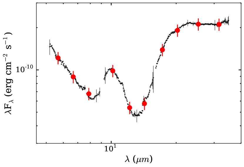
Figure 1: Derredened IRS spectrum of SZ Cha. Black dots show the CASSIS spectrum of this source (after bad pixels rejection) with the corresponding error bars. The binned spectrum and assumed uncertainties are shown as red, larger dots. It properly traces the shape of original data including the silicate feature at 10 $\mu$m.

3 Modeling

We aimed at modeling the selected targets and quantifying the impact of adding photometric Herschel data to this process. For this reason, we used two different datasets for each object. The first dataset comprises the available data from 2MASS, IRAC1/IRAC2, and the binned IRS spectra. The second dataset also includes the Herschel photometry.

We used the MCFOST software (Pinte et al., 2006; Pinte et al., 2009) version 2.19 to model these disks. MCFOST is a Monte Carlo-based raytracing code which generates synthetic SEDs and images of circumstellar disks. First, it produces temperature and density maps of the disk using the provided stellar and disk parameters. In this case, we used 10⁷ photons in this step (enough to produce smooth and well-sampled temperature maps of the disks). After this step, a list of wavelengths is provided for MCFOST to calculate the corresponding synthetic monochromatic fluxes. We required 2 000 photons to be received for each wavelength, corresponding to noise levels of 2-3 % in the flux estimates and well below the assumed observational uncertainties (10-20 %).

Our models include seven free parameters: disk dust mass ($M_{dust}$), inner and outer radii ($R_{in}$, $R_{out}$), scale height at 100 AU (H₁₀₀), flaring index ($h$), surface density exponent ($p$), and the maximum grain size ($a_{max}$). Given the complex structures of circumstellar disks, there are several degeneracies and dependencies between these parameters, and some may even be totally unconstrained with the available data. We did not attempt to fit the mineralogy of the disks. Instead, we assumed typical astronomical silicate compositions, and fixed the minimum grain size to 0.01 $\mu$m. A more in-depth study of the mineralogy of these disks would add an important source of complexity to modeling, and we preferred not to include it in our comparative analysis. We chose a power-law index for the surface density profile. More complex structures such as tapered-edge profiles could also be used (e.g. Lynden-Bell & Pringle, 1974), but direct high-resolution observations are required to actually trace the mass distribution in the disk. Following Espaillat et al. (2011), we also fixed the inclination of all disks to 60 °. Although this inclination is somewhat arbitrary, none of these objects show signatures of high-inclination (e.g., silicate features in absorption or under-luminous photospheres). Moreover, for wavelengths $>$ 13 $\mu$m, the mid-IR continuum is almost insensitive to this effect unless the disk is very close to edge-on (Furlan et al., 2006; D’Alessio et al., 2006).

Among the objects in the sample, SZ Cha has NIR excess over the photospheric emission. This feature is characteristic of pre-TDs, sources with an optically thick inner disk, separated from the outer disk by a gap in the radial dust distribution (e.g., Espaillat et al., 2007a). Additionally, CS Cha has no NIR excess but a prominent silicate emission feature at 10 $\mu$m, indicating the presence of optically thin dust in its inner hole. The inner disks of these objects have already been modeled in detail (e.g., Espaillat et al., 2007b; Kim et al., 2009; Manoj et al., 2011) and we do not attempt to fit them: instead, we adopted the parameter results from these previous studies to reproduce the NIR SED shape. The inner disks remained fixed during the fitting process. This may have an impact in our final results, as discussed later in the paper (see Sect. 3.2).

3.1 Methodology

We adopted a Bayesian approach to properly derive confidence intervals for the outer disk parameters. The usage of Bayesian techniques has increased significantly in Astrophysics during the past years, and we do not intend to explain them in detail. Instead, we refer the interested reader to introductory works such as Trotta (2008). Also, this technique has already been applied for modeling circumstellar disks with Herschel data (e.g. Cieza et al., 2011; Harvey et al., 2012; Spezzi et al., 2013), mainly via model grids. Here we describe the adopted fitting procedure.

Bayesian analysis requires that we assign priors to model parameters. While the selection of restrictive priors may have a significant effect on the fitting results, priors are also an important tool to force parameters to remain within certain ranges, avoiding non-physical solutions. We used flat (non-informative) priors for all the parameters, and constrain them to reasonable values for TDs. The prior ranges used were as follows:

• $\log{(M_{dust}/M_{\odot})}$: from -6 to -2,

• $R_{in}$: from 1 AU to $r_{in-out}$,

• $R_{out}$: from $r_{in-out}$ to 500 AU,

• $H_{100}$: from 0.5 to 25 AU,

• $h$: from 0.8 to 1.3,

• $p$: from -2.5 to 1,

• $\log{(a_{max}/\mu{\rm m})}$: from -1 to 4,

where $r_{in-out}$ depends on the target, and is a physically meaningless parameter merely used to avoid the outer disk becoming smaller than the inner one during the evolution of the MCMC. Based on previous results (Kim et al., 2009; Espaillat et al., 2011), we set $r_{in-out}$ to 30, 40, and 50 AU for T25, SZ Cha, and CS Cha respectively. $M_{dust}$ and $a_{max}$ can take values within several orders of magnitude, and hence we chose to explore them in logarithmic scale.

We used a modified version of Markov Chain Monte Carlo methods (MCMC) called ensemble samplers with affine invariance (Goodman & Weare, 2010). This method uses several “walkers” or individual chains to explore the posterior distributions of parameters, and is especially useful when these distributions have complex forms. We used a slightly modified version of the implementation by Foreman-Mackey et al. (2013), and set the stretch parameter of the walk to 1.5, getting acceptance ratios between 10-50% (a good compromise between a random walk and discarding most of the proposed positions in the chain evolution). In every iteration, the chain comprises 100 walkers. We assume Gaussian uncertainties for our observations, and used the corresponding likelihood function.

To avoid dependencies with the distance to the objects, we normalize every model to the $J$ band prior to estimating the likelihood. This should have no impact in our results, since the $J$ band traces photospheric emission in TDs and does not depend on disk parameters (i.e., all models obtained for a given object have always the same $J$ flux).

When available, we set the initial position of the chains around previous results in the literature (Kim et al., 2009; Espaillat et al., 2011). The posterior from MCMCs are only valid once the system has lost memory of their initial values. This can be quantified using the autocorrelation time of the chains, which gives an estimate of the required number of iterations to draw independent samples. For every case, we computed the autocorrelation time for each walker in each parameter, and took the maximum value for conservative purposes. We then left the system evolve for five autocorrelation times (typically $\sim$ 500 iterations). At this point, the results are independent of the initial position, and the chain is now sampling the posterior distribution. We then estimated the posterior function with other five autocorrelation times (i.e., 50 000 models, the result of the 500 iterations per 100 walkers used).

3.2 Model caveats and limitations

Simple parametric modeling like the one used in this paper offers several advantages (e.g., we can compute synthetic SEDs of complex disks without analytic solution), but it also suffers from some caveats that should be kept in mind. Parametric modeling does not guarantee that a combination of parameters is physically consistent, which we have tried to attenuate using physically meaningful priors. We have not included more complex features/models, such as puffed up inner rims (e.g. Dullemond & Dominik, 2004; Isella & Natta, 2005), non-axisymmetric inhomogeneities (e.g., Andrews et al., 2011; van der Marel et al., 2013), several radial gaps (as ALMA observations have revealed for HL Tau, ALMA Partnership et al., 2015), or fitting for the inner disks (e.g., Espaillat et al., 2010, 2011) or mineralogies. Nonetheless, some of these caveats are likely to have little or no impact in our final results, if applicable at all. The homogeneous treatment of data and fitting procedure used provides a good understanding of the value of each dataset, and an adequate frame for comparing the obtained distributions.

4 Results

4.1 Fitting results without Herschel data

We first use the dataset without Herschel data to explore which parameters can be constrained with NIR/MIR information. The posterior distributions for the three targets are shown in Fig. 2, and the obtained values in Table 3. MCMCs also allow to study degeneracies between different parameters by plotting the chains in different 2-D projections. The degeneracies are very similar in all cases, as revealed by the cornerplots in the Appendix (Figs. 4 to 6).

The following conclusions can be drawn from the obtained posterior distributions for the model parameters by analyzing 5-95 % confidence intervals (Fig. 3):

• The inner radius ($R_{in}$) can be constrained within 5-20 AU for all three targets, corresponding to relative uncertainties between 80-120 %. This is likely due to the fact that most of the NIR/MIR emission arises in the exposed wall, hence probing the location of this parameter.

• NIR/MIR photometry allows to calculate the scale height ($H_{100}$) with uncertainties within 10 AUs. This is expected, since different scale heights modify the amount of stellar flux intercepted by the disk, changing the emission from the inner disk

• The dust mass ($M_{dust}$) and the rest of the geometrical parameters ($R_{out}$, $h$, and $p$) show little or no constraint at all with NIR/MIR data alone.

• Special attention should be paid to the two-peak distributions obtained for $a_{max}$. Any observation at a given wavelength $\lambda$ is only sensible to emission from grains of size $a\sim\lambda$ (Draine, 2006). If we allow $a_{max}$ to take small enough values ($<10\,\mu$m), it could produce substantial changes in the SED and therefore play a role in the modeling, which may explain the double peaked posterior distributions. Although much larger grains are generally expected in disks, this dataset is not enough to resolve this effect if we allow $a_{max}$ to take small enough values.

• As expected, several degeneracies appear in all cases, the most obvious being inner radius with scale height, and scale height with flaring index. In some cases, the inner radius also shows a dependence with the maximum grain size, in relation with the previous point.

4.2 Fitting results with Herschel data

We repeated the modeling procedure including Herschel data for the three selected TDs. As in the previous case, the resulting posterior distributions are shown in Fig. 2, and full corner plots in the Appendix (Figs. 4 to 6). Fig. 3 show the observed SEDs and modeling results, and Table 3 provides the obtained numerical values.

• Compared to the Spitzer-only fit, the addition of Herschel data makes an important difference for $M_{dust}$ and $R_{in}$. For the latter, the posterior distributions are narrowed down by a factor of two with respect to the previous case, with the 5-95 % confidence intervals covering 5-10 AUs, or relative errors of 45-60 % . For the dust mass, the improvement is substantial, constraining its value within one order of magnitude for SZ Cha and T25, and a broader distribution ($\sim$2 dex) for CS Cha, given that it lacks a detection at 500 $\mu$m.

• The scale height ($H_{100}$) is better constrained with Herschel for SZ Cha and CS Cha, reducing the uncertainties by a factor of $\sim$ 2. For T25, there is no additional improvement, We note that, despite this, the combination of $R_{in}$, $h$, and $H_{100}$ yield very similar values of the scale height at the inner radius, with improvements in uncertainty below of 1 AU or less.

• For the rest of disk geometry parameters, there is no real improvement compared to the Spitzer-only fit. We do however see marginal evidence of anomalous outer disks in these objects, when combining the preferred values of $h$ and $p$, specially for SZ Cha and CS Cha. We will discuss this in the following section.

• Herschel data break the two-peak degeneracy in the maximum grain size ($a_{max}$). Although they are not enough to provide a real estimate of this value, they inform that this value is very likely larger than 100 $\mu$m in all cases.

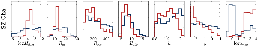
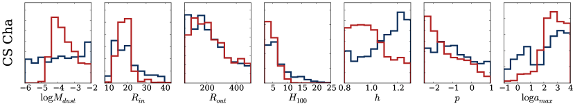
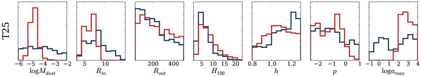
Figure 2: Posterior distributions of the free parameters for the considered transitional disks. Results without Herschel data are shown in blue, those including Herschel in red.

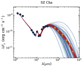
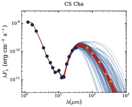
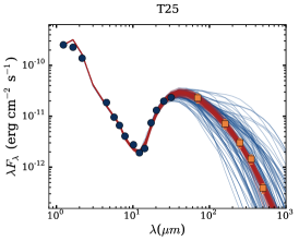
Figure 3: Derredened SEDs for the transitional disks in this study. Photometric data from previous studies are shown as blue solid circles, Herschel measurements as orange squares. Uncertainties are plotted, although in several cases are smaller than symbol sizes. We also show 100 randomly selected models from the obtained posterior distributions for each case: blue lines correspond to fitting without Herschel data, red lines are the resulting models when including Herschel photometry. This gives an idea on the total uncertainties in the SEDs of the modeled disks.

Table 3: Results of the MCMC fitting for the seven free parameters considered. We tabulate the obtained median value and the 5 % and 95 % confidence intervals. For each column, results obtained without Herschel data (left) and with them (right) are provided.

Object	$\log{M_{dust}}$	$R_{in}$	$R_{out}$	$H_{100}$
	($\log{M_{\odot}}$)	(AU)	(AU)	(AU)
	no Herschel | with Herschel	no Herschel | with Herschel	no Herschel | with Herschel	no Herschel | with Herschel
SZ Cha	$-3.6_{-2.0}^{+1.5}$ $|$ $-3.4_{-0.5}^{+1.0}$	$17_{-7}^{+7}$ $|$ $13_{-4}^{+2}$	$220_{-170}^{+240}$ $|$ $200_{-120}^{+240}$	$8.8_{-3.1}^{+5.0}$ $|$ $7.6_{-1.7}^{+2.9}$
CS Cha	$-3.8_{-2.0}^{+1.6}$ $|$ $-3.8_{-0.8}^{+1.4}$	$19_{-7}^{+16}$ $|$ $18_{-5}^{+6}$	$200_{-130}^{+250}$ $|$ $210_{-140}^{+250}$	$5.8_{-2.7}^{+10.4}$ $|$ $4.6_{-1.3}^{+4.2}$
T25	$-4.2_{-1.6}^{+2.0}$ $|$ $-4.7_{-0.5}^{+0.6}$	$8.0_{-3.4}^{+4.4}$ $|$ $6.6_{-2.1}^{+1.6}$	$190_{-150}^{+260}$ $|$ $220_{-160}^{+250}$	$6.0_{-3.0}^{+8.1}$ $|$ $7.6_{-3.8}^{+9.0}$

Object	$h$	$p$	$\log{a_{max}}$
	-	-	($\log{\mu m}$)
	no Herschel | with Herschel	no Herschel | with Herschel	no Herschel | with Herschel
SZ Cha	$1.1_{-0.3}^{+0.2}$ $|$ $1.0_{-0.2}^{+0.2}$	$-1.0_{-1.3}^{+1.7}$ $|$ $-1.6_{-0.8}^{+1.9}$	$0.2_{-0.6}^{+3.5}$ $|$ $2.9_{-1.1}^{+1.0}$
CS Cha	$1.1_{-0.3}^{+0.2}$ $|$ $1.0_{-0.2}^{+0.3}$	$-1.1_{-1.3}^{+1.8}$ $|$ $-1.6_{-0.9}^{+1.9}$	$2.4_{-2.8}^{+1.5}$ $|$ $2.7_{-2.1}^{+1.1}$
T25	$1.1_{-0.3}^{+0.1}$ $|$ $1.1_{-0.2}^{+0.2}$	$-1.0_{-1.3}^{+1.8}$ $|$ $-1.1_{-1.2}^{+1.1}$	$1.8_{-2.3}^{+2.0}$ $|$ $2.9_{-0.9}^{+1.0}$

5 Discussion

5.1 Masses and inner radii

The estimate of two free parameters in our models have been found to improve significantly when including Herschel data: the disk dust mass and its inner radius.

The mass of the disk is one of the most important parameters for planet formation. It determines the available reservoir to build up planets and for accretion on the central star, and can even modify the planet formation mechanism (the disk instability scenario requires high $M_{disk}/M_{*}$ values, e.g., Lodato et al., 2005). Although the bulk of mass in protoplanetary disks is in gaseous form, photometric IR data are only sensitive to dust emission, which are efficient radiation absorbers and emitters. Hence, only the dust mass can be (partially) constrained with the presented data. A total disk mass estimate requires either gas mass measurements (e.g., ¹³CO, C¹⁸O, Panić et al., 2008) or assumptions on the gas-to-dust ratio. Since the former is only available for a few disks, most authors assume a typical gas-to-dust ratio of 100. We adopt this value for comparison with previous studies, but are aware that such an assumption may not hold true in many cases, since the gas-to-dust ratio is likely to change with time and from one source to another (Thi et al., 2010, 2014) . Regardless of this, our results show that Herschel data can be used to constrain the mass of dust in these (pre-)TDs within $\sim$ one order of magnitude for the 5-95 % confidence interval, which is a tremendous improvement with respect to MIR photometry only and opens the exciting possibility of studying this parameter for the large number of sources observed with Herschel and missing mm observations. As expected and illustrated by the case of CS Cha, the longest wavelengths (SPIRE 500 $\mu$m) are the most important ones to constrain the mass, as the disk becomes progressively optically thin at longer wavelengths.

The inner radii of the disks are also significantly better constrained with Herschel data, decreasing previous uncertainties by a factor of two. This improvement arises from PACS data, which narrow down the location of the peak emission, directly related with the illuminated inner wall. Using unbinned IRS spectra could also provide even better estimates for these values. Nevertheless, our results results show that at least some information about this parameter is contained in Herschel data.

We also compare the obtained values with previous estimates in the literature. There are four main studies which can be used for this purpose: Kim et al. (2009), Espaillat et al. (2011), Ubach et al. (2012), and Rodgers-Lee et al. (2014). Kim et al. (2009) presented detailed modeling of the IRS spectra of TDs in Chamaeleon I with an analytic model, including emission from the optically thin disk and wall and emission from the outer disk treated as a blackbody. In Espaillat et al. (2011), the authors used a more complex irradiated disk model (D’Alessio et al., 2006) including shadowing of the outer disk by the inner disk (Espaillat et al., 2010) to analyze variability in the IRS spectra of several TDs. Ubach et al. (2012) presented 3 and 7 mm interferometric measurements of SZ Cha and CS Cha, providing disk mass estimates. More recently, Rodgers-Lee et al. (2014) performed a multiwavelength study of Chamaeleon I including Herschel data from Winston et al. (2012), and analyzed TDs in the region with a physical disk model (Beckwith et al., 1990).,

• Mass values computed with two different methods are available for all the targets: via mm data (Kim et al., 2009; Ubach et al., 2012; Rodgers-Lee et al., 2014) and via the accretion-to-viscosity ratio (Espaillat et al., 2011) following D’Alessio et al. (1998). Our results are in very good agreement with these previous values, and match within a factor of two for most cases except for the mass value of CS Cha in Espaillat et al. (2011), SZ Cha in Ubach et al. (2012), and T25 from Kim et al. (2009). In the former case, a value of 0.3 $M_{\odot}$ is quoted, more than one order of magnitude larger than our estimated median value (0.015 $M_{\odot}$) but within the 95 % confidence interval range. Therefore, the two results are consistent within uncertainties. Additionally, the value in Espaillat et al. (2011) depends on the disk viscosity, which is usually largely uncertain and could account for this difference. In the case of SZ Cha, our results for the 5-95 % interval yields values of 1.3$\times 10^{-2}$$-$0.4 $M_{\odot}$, while Ubach et al. (2012) obtained a total disk mass of 9.4$\times 10^{-3}$ $M_{\odot}$. Considering that this measurement is also subject to uncertainties (between a factor of two to ten, according to Ubach et al., 2012), then our results match completely within the uncertainty range. For T25, Kim et al. (2009) estimate a 0.007 $M_{\odot}$ disk mass via 1.3 mm fluxes from Henning et al. (1993). Our study yields a disk mass for T25 of 0.002 $M_{\odot}$, with their value lying just at the border of the corresponding confidence interval. However, as noted by Rodgers-Lee et al. (2014), the 1.3 mm flux value in Kim et al. (2009) for T25 is an upper limits, and therefore their mass estimates should be considered as such, solving the discrepancy. Rodgers-Lee et al. (2014) also found that Herschel data within the 160-500 $\mu$m range can be used to estimate disk masses within a factor of 3 without the need of detailed modeling. Our results show larger uncertainties ($\sim$ one-two orders of magnitude for the 5-95 % confidence interval), stressing the importance of considering other sources of uncertainties (such as disk temperature and composition) to compute realistic confidence intervals of model parameters.

• Disk inner radii estimates are available both in Kim et al. (2009) and Espaillat et al. (2011). Our results using MIR data only are in general good agreement with their values, with the discrepancy of CS Cha. These two works estimated its inner disk radii to be 41 and 38 AU, respectively, while we obtain $19_{-7}^{+16}$ AU with similar data (i.e., excluding Herschel). Their results fall outside the 5-95 % confidence intervals derived in this study. Two different effects can explain this apparent discrepancy. First, there is no uncertainty estimation in the quoted studies: if we assume their results to have similar uncertainties to ours, the resulting distributions would overlap significantly and yield consistent values. Additionally, these two works included more complex dust compositions, which can modify the grain emissivity and therefore change the location of the inner radius. We also note that Kim et al. (2009) estimated a 29 AU gap for T25, although the improved estimate of 18 AU in Espaillat et al. (2011) is completely consistent with ours.

The mass ranges of these TDs are similar to those of Class II disks in other star-forming regions (e.g., Ophiuchus, Taurus, Andrews et al., 2010, 2013), a result already found by Andrews et al. (2011) for 12 TDs observed with sub-mm interferometry. This is somehow intriguing: if TDs are an evolved stage of protoplanetary disks, then we would expect them to have significantly lower masses. In fact, other works found TDs to have masses even higher than those of Class II sources (Najita et al., 2007, 2015). If that is the case, TDs (at least classical ones, those with large holes in their dust distribution) could be the evolution of high-mass disks which have formed multiple giant planets (explaining their gaps, Zhu et al., 2011), and not a general evolutionary stage for all protoplanetary disks.

We also compare these values with that of the Minimum Mass Solar Nebula (MMSN, Hayashi, 1981), the minimum mass required to form the Solar System. A typical value of this quantity is $\sim$0.02 $M_{\odot}$ (Davis, 2005; Desch, 2007). Both SZ Cha and CS Cha are above or close to this value, meaning that despite being in a transitional stage, they still have enough mass to form a significant number of planets (although this does not guarantee that planet formation will take place in the future).

5.2 Anomalous outer disks

We find a general trend for flaring indexes ($h$) close to $\sim$ 1, slightly smaller than those usually found in protoplanetary disks ($\sim$ 1.1-1.3, e.g., Chiang & Goldreich, 1997; Olofsson et al., 2013). Additionally, Herschel data suggest strongly negative surface density profiles, with no peak at -1, as typically assumed and found in protoplanetary disks (e.g., Andrews et al., 2009). Surprisingly, the obtained values are closer to that of the estimated for the MMSN (i.e. -1.5, -2.2, Hayashi, 1981; Desch, 2007).

These two results are likely accounting for an observed trend in the SEDs of these three targets: they have a significant amount of excess in the MIR range up to 70-100 $\mu$m (already hinted in Cieza et al., 2011; Ribas et al., 2013), but their slopes between 250-500 $\mu$m are bluer than those of typical Class II disks. This was found in Ribas et al. (2013) when comparing the SEDs of (pre-)TDs in Chamaeleon I with the median SED of the Chamaeleon I and II regions. The obtained steep surface density profiles and flaring indexes reduce the flux at longer wavelengths (SPIRE), and increase it at shorter wavelengths (20-150 $\mu$m, IRS, MIPS, and PACS). Low flaring indexes could arise if significant dust settling towards the mid-plane has already occurred in these disks, reducing the disk surface exposed to the stellar radiation specially in the outer regions of the disk. On the other hand, smaller (more negative) surface densities imply that more mass is located close to the star, leaving a fainter outer disk which will emit poorly in the FIR regime. Combined, these results suggest that the modeled (pre-)TDs have anomalous outer disks compared to Class II objects. The same fact is found for the T Cha TD using Herschel data (Cieza et al., 2011) and in the Lupus region (Bustamante et al., 2015), reinforcing this idea.

We stress that this interpretation is based on weak evidence and a very small sample, and should be considered with caution: the posterior functions of these parameters are broad and do not discard canonical values, but simply make them slightly less probable. The hint of this phenomenon arises from the fact that the three sources under study show this same marginal behavior. The usage of tapered-edge surface densities profiles (e.g., Lynden-Bell & Pringle, 1974; Hartmann et al., 1998) or puffed up inner rims (e.g., Dullemond et al., 2001) may also help explaining the anomalous SED slopes. Further evidence for flattened disks can be obtained by combining accretion and [OI] measurements. Keane et al. (2014) found the Herschel [OI] flux of 26 TDs to be $\sim$2 times fainter than those of full disks, suggesting smaller gas-to-dust ratios compared to Class II disks, or smaller flaring indices. If the first scenario is ruled out by detecting significant gas reservoirs (via accretion signatures), then the flatter disks explanation would be favored. Resolved ALMA observations of larger samples of (pre-)TDs and full disks will reveal their real gas content and probe their structure, shedding light on this open issue.

6 Conclusions

We use Herschel photometry of three TDs in the Chamaeleon I star-forming region to perform detailed MCMC modeling of their SEDs and study the impact of Herschel data in the obtained results. We find that Herschel photometry, specially from the SPIRE instrument, can be used to constrain the dust mass in disks within one order of magnitude, as shown by the obtained posterior distributions. Herschel data can also help narrowing down the location of the inner radius of the disk. Our results are in good agreement with previous studies.

For the modeled targets, we find disk masses comparable to those of Class II sources in other star-forming regions. Because TDs are likely to represent a more evolved stage of disk evolution, the fact that they do not have significantly lower masses could suggest that the typical transitional class (i.e., disks with large gaps in their dust distributions) is the evolutionary outcome of massive Class II sources, with enough mass to form several giant planets which may have cleared their inner regions. Additionally, we find marginal hints of some dust settling and/or stepper surface density profiles in TDs than in protoplanetary disks. However, this result is tentative and requires further analysis. A larger sample of TDs, combined with gas and accretion measurements as well as resolved images of these targets could help solving this issue and shed light on the origin of TDs and their real connection with planets.

Given the importance of disk masses for planet formation theories, the results obtained in this study open exciting new options to study this parameter for a large number of targets which lack (sub)mm observations but are present in the Herschel Science Archive. Further calibration of these values could also be achieved with more precise disk mass measurements from mm observations. Such a large scale study could identify underlying relations between the stellar properties, disk masses, and the characteristics of planetary systems.

Appendix A Cornerplots for the considered transitional disks

In this appendix, we provide the cornerplots obtained with the adopted MCMC procedure (Figs. 4 to 6).

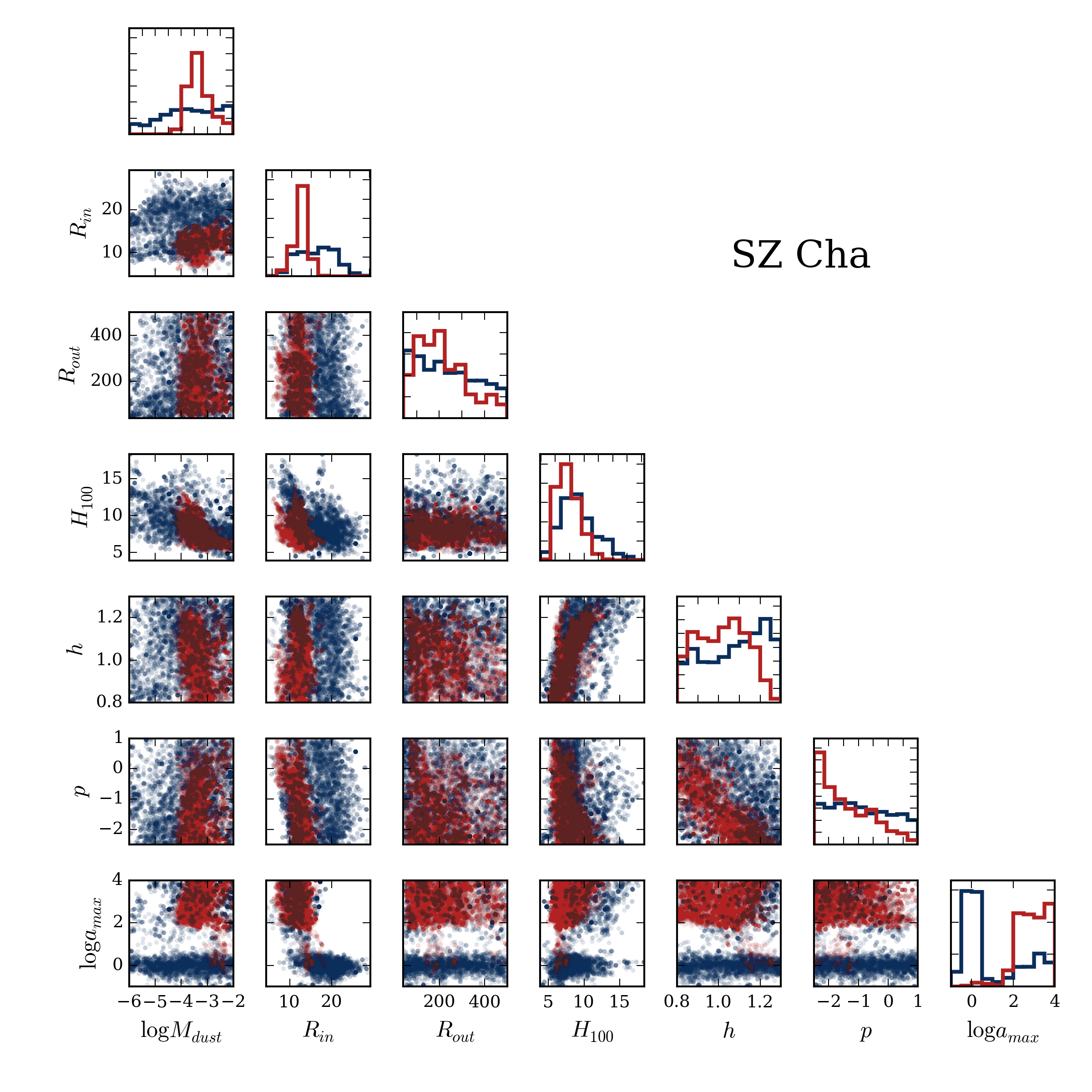
Figure 4: Cornerplot for SZ Cha. Histograms show the posterior distribution for each free parameter, scatter plots display the position of each chain in two parameter spaces to trace degeneracies. The results without Herschel data are shown in blue, those including Herschel in red.

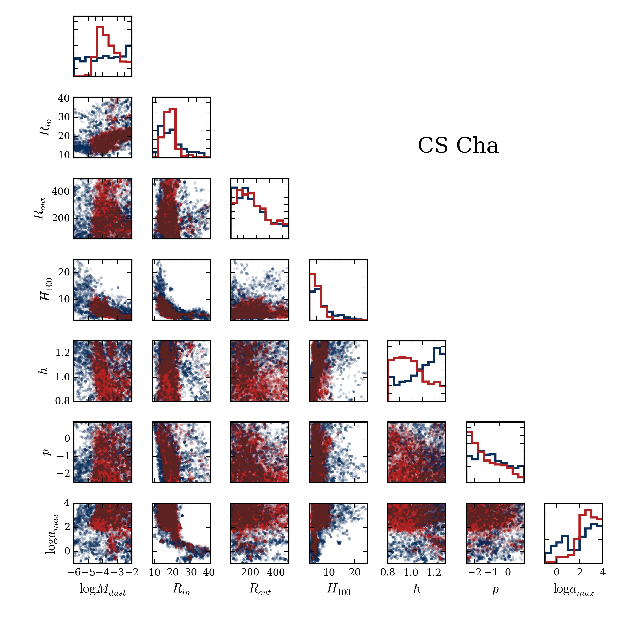
Figure 5: Cornerplot for CS Cha. Scheme and colors as in Fig. 4.

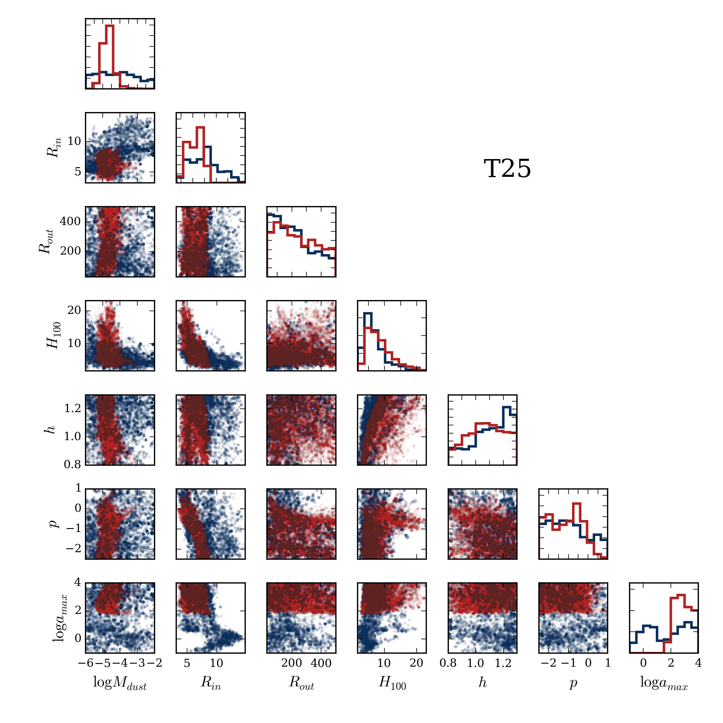
Figure 6: Cornerplot for T25. Scheme and colors as in Fig. 4.

References

- ALMA Partnership et al. (2015) ALMA Partnership et al., 2015, ApJ, 808, L3
- Alexander et al. (2014) Alexander R., Pascucci I., Andrews S., Armitage P., Cieza L., 2014, Protostars and Planets VI, pp 475–496
- André et al. (2010) André P., et al., 2010, A&A, 518, L102
- Andrews & Williams (2005) Andrews S. M., Williams J. P., 2005, ApJ, 631, 1134
- Andrews et al. (2009) Andrews S. M., Wilner D. J., Hughes A. M., Qi C., Dullemond C. P., 2009, ApJ, 700, 1502
- Andrews et al. (2010) Andrews S. M., Wilner D. J., Hughes A. M., Qi C., Dullemond C. P., 2010, ApJ, 723, 1241
- Andrews et al. (2011) Andrews S. M., Wilner D. J., Espaillat C., Hughes A. M., Dullemond C. P., McClure M. K., Qi C., Brown J. M., 2011, ApJ, 732, 42
- Andrews et al. (2013) Andrews S. M., Rosenfeld K. A., Kraus A. L., Wilner D. J., 2013, ApJ, 771, 129
- Balog et al. (2014) Balog Z., et al., 2014, Experimental Astronomy, 37, 129
- Beckwith et al. (1990) Beckwith S. V. W., Sargent A. I., Chini R. S., Guesten R., 1990, AJ, 99, 924
- Belloche et al. (2011) Belloche A., et al., 2011, A&A, 527, A145
- Birnstiel et al. (2012) Birnstiel T., Andrews S. M., Ercolano B., 2012, A&A, 544, A79
- Bustamante et al. (2015) Bustamante I., Merín B., Ribas Á., Bouy H., Prusti T., Pilbratt G. L., André P., 2015, A&A, 578
- Chiang & Goldreich (1997) Chiang E. I., Goldreich P., 1997, ApJ, 490, 368
- Cieza et al. (2011) Cieza L. A., et al., 2011, ApJ, 741, L25
- D’Alessio et al. (1998) D’Alessio P., Cantö J., Calvet N., Lizano S., 1998, ApJ, 500, 411
- D’Alessio et al. (2006) D’Alessio P., Calvet N., Hartmann L., Franco-Hernández R., Servín H., 2006, ApJ, 638, 314
- Davis (2005) Davis S. S., 2005, ApJ, 627, L153
- Desch (2007) Desch S. J., 2007, ApJ, 671, 878
- Draine (2006) Draine B. T., 2006, ApJ, 636, 1114
- Dullemond & Dominik (2004) Dullemond C. P., Dominik C., 2004, A&A, 417, 159
- Dullemond et al. (2001) Dullemond C. P., Dominik C., Natta A., 2001, ApJ, 560, 957
- Espaillat et al. (2007a) Espaillat C., et al., 2007a, ApJ, 664, L111
- Espaillat et al. (2007b) Espaillat C., Calvet N., D’Alessio P., Hernández J., Qi C., Hartmann L., Furlan E., Watson D. M., 2007b, ApJ, 670, L135
- Espaillat et al. (2010) Espaillat C., et al., 2010, ApJ, 717, 441
- Espaillat et al. (2011) Espaillat C., Furlan E., D’Alessio P., Sargent B., Nagel E., Calvet N., Watson D. M., Muzerolle J., 2011, ApJ, 728, 49
- Espaillat et al. (2014) Espaillat C., et al., 2014, preprint, (arXiv:1402.7103)
- Foreman-Mackey et al. (2013) Foreman-Mackey D., Hogg D. W., Lang D., Goodman J., 2013, PASP, 125, 306
- Furlan et al. (2006) Furlan E., et al., 2006, ApJS, 165, 568
- Furlan et al. (2011) Furlan E., et al., 2011, The Astrophysical Journal Supplement Series, 195, 3
- Goodman & Weare (2010) Goodman J., Weare J., 2010, Comm. App. Math. Comp. Sci., 5, 65
- Griffin et al. (2010) Griffin M. J., et al., 2010, A&A, 518, L3
- Guenther et al. (2007) Guenther E. W., Esposito M., Mundt R., Covino E., Alcalá J. M., Cusano F., Stecklum B., 2007, A&A, 467, 1147
- Hartmann et al. (1998) Hartmann L., Calvet N., Gullbring E., D’Alessio P., 1998, ApJ, 495, 385
- Harvey et al. (2012) Harvey P. M., et al., 2012, ApJ, 755, 67
- Hayashi (1981) Hayashi C., 1981, Progress of Theoretical Physics Supplement, 70, 35
- Henning et al. (1993) Henning T., Pfau W., Zinnecker H., Prusti T., 1993, A&A, 276, 129
- Houck et al. (2004) Houck J. R., et al., 2004, ApJS, 154, 18
- Indebetouw et al. (2005) Indebetouw R., et al., 2005, ApJ, 619, 931
- Ireland & Kraus (2008) Ireland M. J., Kraus A. L., 2008, ApJ, 678, L59
- Isella & Natta (2005) Isella A., Natta A., 2005, A&A, 438, 899
- Keane et al. (2014) Keane J. T., et al., 2014, ApJ, 787, 153
- Kim et al. (2009) Kim K. H., et al., 2009, ApJ, 700, 1017
- Lebouteiller et al. (2011) Lebouteiller V., Barry D. J., Spoon H. W. W., Bernard-Salas J., Sloan G. C., Houck J. R., Weedman D. W., 2011, ApJS, 196, 8
- Lodato et al. (2005) Lodato G., Delgado-Donate E., Clarke C. J., 2005, MNRAS, 364, L91
- Luhman (2004) Luhman K. L., 2004, ApJ, 602, 816
- Luhman (2007) Luhman K. L., 2007, ApJS, 173, 104
- Luhman et al. (2008) Luhman K. L., et al., 2008, ApJ, 675, 1375
- Lynden-Bell & Pringle (1974) Lynden-Bell D., Pringle J. E., 1974, MNRAS, 168, 603
- Manoj et al. (2011) Manoj P., et al., 2011, ApJS, 193, 11
- Men’shchikov et al. (2012) Men’shchikov A., André P., Didelon P., Motte F., Hennemann M., Schneider N., 2012, A&A, 542, A81
- Merín et al. (2010) Merín B., et al., 2010, ApJ, 718, 1200
- Muzerolle et al. (2009) Muzerolle J., et al., 2009, ApJ, 704, L15
- Nagel et al. (2012) Nagel E., Espaillat C., D’Alessio P., Calvet N., 2012, ApJ, 747, 139
- Najita et al. (2007) Najita J. R., Strom S. E., Muzerolle J., 2007, MNRAS, 378, 369
- Najita et al. (2015) Najita J. R., Andrews S. M., Muzerolle J., 2015, MNRAS, 450, 3559
- Olofsson et al. (2013) Olofsson J., Szűcs L., Henning T., Linz H., Pascucci I., Joergens V., 2013, A&A, 560, A100
- Ott (2010) Ott S., 2010, in Mizumoto Y., Morita K.-I., Ohishi M., eds, Astronomical Society of the Pacific Conference Series Vol. 434, Astronomical Data Analysis Software and Systems XIX. p. 139 (arXiv:1011.1209)
- Panić et al. (2008) Panić O., Hogerheijde M. R., Wilner D., Qi C., 2008, A&A, 491, 219
- Pearson et al. (2014) Pearson C., et al., 2014, Experimental Astronomy, 37, 175
- Pilbratt et al. (2010) Pilbratt G. L., et al., 2010, A&A, 518, L1
- Pinte et al. (2006) Pinte C., Ménard F., Duchêne G., Bastien P., 2006, A&A, 459, 797
- Pinte et al. (2009) Pinte C., Harries T. J., Min M., Watson A. M., Dullemond C. P., Woitke P., Ménard F., Durán-Rojas M. C., 2009, A&A, 498, 967
- Poglitsch et al. (2010) Poglitsch A., et al., 2010, A&A, 518, L2
- Ribas et al. (2013) Ribas Á., et al., 2013, A&A, 552, A115
- Rodgers-Lee et al. (2014) Rodgers-Lee D., Scholz A., Natta A., Ray T., 2014, MNRAS, 443, 1587
- Roussel (2013) Roussel H., 2013, PASP, 125, 1126
- Spezzi et al. (2013) Spezzi L., et al., 2013, A&A, 555, A71
- Taylor (2005) Taylor M. B., 2005, in Shopbell P., Britton M., Ebert R., eds, Astronomical Society of the Pacific Conference Series Vol. 347, Astronomical Data Analysis Software and Systems XIV. p. 29
- Thi et al. (2010) Thi W.-F., et al., 2010, A&A, 518, L125
- Thi et al. (2014) Thi W.-F., et al., 2014, A&A, 561, A50
- Trotta (2008) Trotta R., 2008, Contemporary Physics, 49, 71
- Ubach et al. (2012) Ubach C., Maddison S. T., Wright C. M., Wilner D. J., Lommen D. J. P., Koribalski B., 2012, MNRAS, 425, 3137
- Whittet et al. (1997) Whittet D. C. B., Prusti T., Franco G. A. P., Gerakines P. A., Kilkenny D., Larson K. A., Wesselius P. R., 1997, A&A, 327, 1194
- Williams & Cieza (2011) Williams J. P., Cieza L. A., 2011, ARA&A, 49, 67
- Winston et al. (2009) Winston E., et al., 2009, AJ, 137, 4777
- Winston et al. (2012) Winston E., et al., 2012, A&A, 545, A145
- Zhu et al. (2011) Zhu Z., Nelson R. P., Hartmann L., Espaillat C., Calvet N., 2011, ApJ, 729, 47
- van der Marel et al. (2013) van der Marel N., et al., 2013, Science, 340, 1199