Gauge invariant theories of linear response for strongly correlated superconductors

Abstract

We present a general diagrammatic theory for determining consistent electromagnetic response functions in strongly correlated fermionic superfluids. The general treatment of correlations beyond BCS theory requires a new theoretical formalism not contained in the current literature. Among concrete examples are a rather extensive class of theoretical models which incorporate BCS-BEC crossover as applied to the ultra cold Fermi gases, along with theories specifically associated with the high-$T_{c}$ cuprates. The challenge is to maintain gauge invariance, while simultaneously incorporating additional self-energy terms arising from strong correlation effects. Central to our approach is the application of the Ward-Takahashi identity, which introduces collective mode contributions in the response functions and guarantees that the $f$-sum rule is satisfied. We outline a powerful and very general method to determine these collective modes in a manner compatible with gauge invariance. Finally, as an alternative approach, we contrast with the path integral formalism. Here, the calculation of gauge invariant response appears more straightforward. However, the collective modes introduced are essentially those of strict BCS theory, with no modification from correlation effects. Since the path integral scheme simultaneously addresses electrodynamics and thermodynamics, we emphasize that it should be subjected to a consistency test beyond gauge invariance, namely that of the compressibility sum-rule. We show how this sum-rule fails in the conventional path integral approach.

I Introduction

There has been a recent focus in the literature on strongly correlated superconductors and superfluids. This interest has arisen in two different contexts, via ultra cold atomic Fermi gases Taylor ; Randeria1 and via high-$T_{c}$ superconductors YRZ ; Lee ; Norman ; ourreview . A major challenge in studying these two different systems is to arrive at correct expressions for the electromagnetic (EM) properties, such as the superfluid density and the density-density correlation function, which characterize superconductors and superfluids.

In strict BCS theory there are two different conventional techniques for addressing electromagnetic response while ensuring gauge invariance: the path integral Altland ; Yakovenko ; Kitagawa and the Ward-Takahashi identity Nambu . The first of these methods depends on the derivation of a generating functional while the second depends on the form of the diagrammatic self-energy. This body of work has enabled a complete understanding of the gauge invariant electromagnetic response at the BCS level. It does not, however, answer the important questions about how to incorporate stronger correlation effects.

Studies of high-$T_{c}$ superconductors, which necessarily require a beyond-BCS formalism, are better suited to the Ward-Takahashi based approach. These studies focus on different models for the self-energy associated with a normal state that includes pairing, known as the pseudogap phase YRZ ; Lee ; Norman ; ourreview . This correlation contribution to the self-energy has been extensively characterized arpesstanford above the transition temperature $T_{c}$. In the superfluid phase, presumably one adds to this normal state self-energy ourreview ; YRZ an additional BCS self energy contribution. The challenge in studying strongly correlated superfluids, however, is ensuring gauge invariance. This means that the self-consistent collective modes, compatible with gauge invariance, must be properly included. For an arbitrary strongly-correlated self-energy, beyond the BCS-level theory, there is no general diagrammatic procedure to ensure both of these conditions.

In this paper we show that the self-energy and the gap equation provide all the ingredients required to unambiguously establish the exact electrodynamic response at all temperatures. Our main goals are:

(i) To show how to arrive at the exact gauge invariant electromagnetic response of strongly correlated superfluids. This is based on a fairly general form of the self-energy and on the Ward-Takahashi identity.

(ii) To provide a powerful method for obtaining the collective modes in a gauge invariant manner for strongly correlated superfluids. This is based on the form of the gap equation, and the vertex derived above in (i).

The electrodynamics of superconductors is also widely addressed via the path integral approach Altland ; Yakovenko ; Kitagawa which requires the introduction of Gaussian level (beyond saddle point) fluctuations. Incorporating gauge invariance is relatively straightforward, which is in large part due to the fact that the collective modes that enter at this level and beyond are those of strict BCS theory ourcompanion . We shall revisit this conventional calculation of response functions at the strict BCS level, while simultaneously considering thermodynamics. We find there is a serious shortcoming that has not previously been identified in the literature. This arises from an inconsistency between electrodynamics and thermodynamics, which is manifested as a failure of the compressibility sum-rule.

Our emphasis here is not on a critique of previous work since, quite generally, in the literature the focus has been on either the thermodynamics Randeria1 or the electrodynamics Altland ; Yakovenko ; Kitagawa , but not on both simultaneously. Nevertheless, the violation of the compressibility sum-rule is a serious shortcoming. The source of this sum-rule violation comes from the fact that the BCS level electrodynamics are derived by incorporating beyond BCS Gaussian fluctuations. This would seem to require that we also include Gaussian fluctuations in the number equation. However, this in fact leads to the failure of the compressibility sum-rule. A detailed discussion of how to implement consistency between electrodynamics and thermodynamics will be presented elsewhere ourcompanion .

It is crucial when studying transport phenomena to ensure that all conservation laws, such as energy, momentum, and charge, are satisfied KadanoffBaym ; Baym . In particular, ensuring gauge invariance, and thus charge conservation, in a superconductor has long been a problem of great importance Anderson ; Kadanoff ; Nambu ; Kulik ; Hao1 . The key insight in the challenge of preserving gauge invariance, even in the presence of a Meissner effect, was the necessity of long wavelength collective excitations Anderson ; Rickayzen . Following this initial insight, a more diagrammatic approach, built around the establishment of gauge invariance in quantum electrodynamics, was developed by Nambu Nambu . Nambu’s method of establishing a gauge invariant electromagnetic response was to set up a gauge invariant vertex at the same level of approximation as the self-energy. He then showed that this leads to a full vertex that satisfies the Ward-Takahashi identity (WTI), a condition equivalent to gauge invariance Ryder .

A modern understanding of the role of gauge invariance in a superconductor is best understood from this field theoretic point of view: collective modes are excitations which restore gauge invariance. In the language of quantum field theory they can be interpreted as the Nambu-Goldstone bosons arising from spontaneous symmetry breaking in the condensed phase. Strictly speaking, in a superconductor or superfluid local gauge invariance is never broken Greiter . Quite generally, the impossibility of breaking local gauge invariance without explicit gauge fixing, at least for abelian gauge fields, was proved early on by Elitzur Elitzur . Rather, due to the presence of a condensate, global phase invariance is spontaneously broken. In the case of a neutral order parameter the excitation spectrum contains a gapless mode, which corresponds to the collectives modes discussed throughout this paper. For a charged order parameter the Goldstone modes couple to the longitudinal degrees of freedom of the gauge field, and are gapped out.

In going beyond the BCS theory of superconductivity it is essential that gauge invariance is maintained in any approximation scheme. Above the transition temperature, in Refs. Peter1 ; Rufus1 the WTI was implemented for a number of different exotic normal phases, which led to a consistent framework for computing all vertex corrections. The challenge in the present paper is then to extend this body of work and formulate a gauge invariant theory below the transition temperature. In this context, Ref. Hao2 used the WTI to formulate a gauge invariant response for a specific BCS-BEC approximation valid at all temperatures. This theory accounted for non-condensed fermionic pairs by adding a $t$-matrix self-energy to the standard BCS self-energy. Inspired by this work, in this paper we will use the WTI to study a broader class of theories, addressed in the context of high $T_{c}$ superconductors and atomic Fermi superfluids, which are based on an extension of a BCS based self-energy. Within these approaches we go beyond the pioneering work of Nambu and show by extending the method of Ref. Hao2 , that both the full vertex and the collective modes can be explicitly derived for a very general class of strongly correlated superfluids. In particular we derive closed form expressions for the response functions. Theories which belong to this general class include the work of Refs. Peter1 ; Rufus1 along with additional theories such as that proposed in Ref. YRZ , Ref. Lee and Refs. StrinatiPRL ; StrinatiPRB ; StrinatiPRB2 .

II Correlation Effects Beyond BCS theory: Ward-Takahashi Identity

II.1 Kubo formulae

The goal of this section of the paper is to address correlations which go beyond the mean-field BCS theory and, making use of Kubo formulae, arrive at properly gauge invariant linear response functions. We begin by summarizing the Kubo formalism for a many-body theory of interacting fermions. In what follows we shall primarily be concerned with neutral superfluids. Incorporating Coulomb effects can be done through the random phase approximation (RPA) formalism Yakovenko , once the exact response functions are obtained for the neutral system.

In the presence of a weak, externally applied EM field, with four-vector potential $A^{\mu}=(\phi,\mathbf{A})$, the four-current density $J^{\mu}=(\rho,\mathbf{J})$ is given by

$$J^{\mu}(q)=K^{\mu\nu}(q)A_{\nu}(q),$$ (2.1)

where $q=(i\Omega_{m},\mathbf{q})$ is a four-momentum, with a bosonic Matsubara frequency $i\Omega_{m}$. The quantity $K^{\mu\nu}$ is the EM response kernel, which is of principal interest here. Charge conservation $(q_{\mu}J^{\mu}=0)$ implies that the response kernel $K^{\mu\nu}$ must satisfy the condition $q_{\mu}K^{\mu\nu}=0$. The satisfaction of this condition is what we will mean by a gauge invariant many-body theory.

The response kernel $K^{\mu\nu}$ can be written in a general form as schrieffer

$$K^{\mu\nu}(q) =2\sum_{k}G(k_{+})\Gamma^{\mu}(k_{+},k_{-})G(k_{-})\gamma^{\nu}(k_{-},k_{+})$$

$$\quad+\frac{n}{m}\delta^{\mu\nu}(1-\delta_{0\mu}),$$ (2.2)

where the full and bare vertices are $\Gamma^{\mu}(k_{+},k_{-}),$ $\gamma^{\mu}(k_{+},k_{-})$ respectively, and $k_{\pm}\equiv k\pm q/2$ is the incoming (+) or outgoing $(-)$ momenta of a vertex. The particle number is $n$ and $m$ denotes the fermion mass. The full Green’s function is denoted by $G(k)$, which we define in terms of the bare Green’s function, $G_{0}^{-1}(k)=i\omega-\xi_{\mathbf{k}}$, in Eq. (2.4). Here the single particle dispersion is $\xi_{\mathbf{k}}=k^{2}/2m-\mu$, where $\mu$ is the chemical potential.

We now introduce a framework that encapsulates both BCS theory and stronger correlations beyond BCS theory. To understand what is meant by these correlation effects, here we consider a correlated self-energy $\Sigma_{\mathrm{corr}}(k)$. In order to simultaneously describe a wide variety of theories, we define the partially dressed Green’s function

$$\left(G_{0}^{\alpha}\right)^{-1}(k)=G_{0}^{-1}(k)-\alpha\Sigma_{\mathrm{corr}}(k).$$ (2.3)

This depends on the strong correlation contribution to the self-energy $\Sigma_{\mathrm{corr}}$ for $\alpha=1$, and does not include strong correlation effects for $\alpha=0$. The fermionic Green’s function is then given by Dyson’s equation

$$G^{-1}(k)=G_{0}^{-1}(k)-\Sigma(k),$$ (2.4)

where the self-energy consists of two terms:

$$\Sigma(k)=\Sigma_{\mathrm{corr}}(k)-|\Delta_{\mathrm{sc}}|^{2}G^{\alpha}_{0}(-k),$$ (2.5)

for a superconducting order parameter $\Delta_{\mathrm{sc}}$. Equivalently, $\Sigma(k)=\Sigma_{\mathrm{corr}}(k)+\Sigma_{\mathrm{sc}}(k)$, where $\Sigma_{\mathrm{sc}}(k)=-|\Delta_{\mathrm{sc}}|^{2}G^{\alpha}_{0}(-k)$ is the superconducting self-energy.

Finally, the gap equation can be written YRZ ; ourreview as $1-g\sum_{k}G^{\alpha}_{0}(-k)G(k)=0.$ Multiplying both sides of this equation by $\Delta_{\mathrm{sc}}$, we obtain

$$\Delta_{\mathrm{sc}}/g=\sum_{k}\Delta_{\mathrm{sc}}G^{\alpha}_{0}(-k)G(k)\equiv\sum_{k}F_{\mathrm{sc}}(k).$$ (2.6)

In this expression the anomalous Green’s function $F_{\mathrm{sc}}(k)$ has dependence on $\Sigma_{\mathrm{corr}}(k)$ via $G_{0}^{\alpha}(k)$ and $G(k)$, and there is also implicit dependence on $\alpha$ through $G_{0}^{\alpha}(k)$.

This represents a fairly generic class of strongly correlated superfluid systems. When $\Sigma_{\mathrm{corr}}=0$ the system reverts to the conventional BCS theory. Thus, the challenge is to include the correlation effects associated with the self-energy $\Sigma_{\mathrm{corr}}$. Models of this sort are associated with the work of Yang, Rice, and Zhang YRZ , and also with the work of Refs. StrinatiPRL ; StrinatiPRB ; StrinatiPRB2 , who address BCS-BEC crossover effects via a $t$-matrix. Also belonging to this class is an alternate $t$-matrix theory of BCS-BEC crossover ourreview ; Hao2 , which, in contrast to the work of Ref. StrinatiPRL , is more directly associated with a BCS-based ground state.

II.2 The Ward-Takahashi identity

In order to derive the gauge invariant EM response, we now apply the Ward-Takahashi identity (WTI). For a quantum field theory with a $U(1)$ gauge symmetry the WTI is an exact relation between the many-body vertex function that appears in correlation functions and the self-energy which enters in the Green’s function. Moreover, as shown in the Supplemental Material Supplement , given a full vertex that satisfies the WTI, the $f$-sum-rule is satisfied and thus charge is conserved.

Given the bare Green’s function $G_{0}(k)$, and the full Green’s function $G(k)$, the WTI constrains the full vertex $\Gamma^{\mu}(k_{+},k_{-})$ so that it satisfies Ryder

$$q_{\mu}\Gamma^{\mu}(k_{+},k_{-}) =G^{-1}(k_{+})-G^{-1}(k_{-}),$$

$$=q_{\mu}\gamma^{\mu}(k_{+},k_{-})+\Sigma(k_{-})-\Sigma(k_{+}).$$ (2.7)

The bare WTI, $q_{\mu}\gamma^{\mu}(k_{+},k_{-})=G_{0}^{-1}(k_{+})-G_{0}^{-1}(k_{-})$, is satisfied for a bare vertex $\gamma^{\mu}(k_{+},k_{-})=(1,\mathbf{k}/m)$. Therefore, given a self-energy $\Sigma(k)$, the above equation provides a constraint which can be used to determine the full vertex.

The WTI is equivalent to self-consistent perturbation theory, and allows one to compute the exact $n$-loop full vertex, given any $n$-loop self-energy. If the self-energy depends on the full Green’s function, then applying the WTI leads to an integral equation for the full vertex of the Bethe-Salpeter form Nozieres . However, if the self-energy depends on only a finite number of bare or partially dressed Green’s functions, then this integral equation terminates, and the full vertex can be obtained exactly. This is the situation with regard to the strong correlation approaches we consider in this paper.

We now turn to the superconducting case. For a superconductor, where gauge invariance is “spontaneously broken”, the presence of a condensate below the transition temperature leads to a more complicated formulation of the WTI. Imposing gauge invariance in the presence of a condensate requires low energy excitations known as collective modes. The explicit form of the collective modes, however, must be derived from the gap equation Hao2 .

The Ward-Takahashi identity is equivalent to requiring that the full vertex be obtained by performing all possible vertex insertions into the self-energy Nambu . Below the transition temperature, however, we must account for the effect of an external (non-dynamical) vector potential $A_{\mu}$ on the self-consistency condition (Eq. (2.6)). This necessitates the introduction of collective mode vertices $\Pi^{\mu}(q)$, $\bar{\Pi}^{\mu}(q)$ in the full vertex, which are inserted into every location of the condensate terms $\Delta_{\mathrm{sc}}$, $\Delta_{\mathrm{sc}}^{*}$, respectively. In the next section we discuss these collective mode vertices in greater detail. As shown in the Supplemental Material Supplement , performing all vertex insertions into the self-energy of Eq. (2.5), and using Eq. (II.2), then gives the full vertex:

$$\Gamma^{\mu} (k_{+},k_{-})=\gamma^{\mu}(k_{+},k_{-})+\Lambda^{\mu}(k_{+},k_{-})$$

$$-\Delta_{\mathrm{sc}}^{*}\Pi^{\mu}(q)G^{\alpha}_{0}(-k_{-})-\Delta_{\mathrm{sc}}\bar{\Pi}^{\mu}(q)G^{\alpha}_{0}(-k_{+})$$

$$-|\Delta_{\mathrm{sc}}|^{2}G^{\alpha}_{0}(-k_{-})G^{\alpha}_{0}(-k_{+})\times$$

$$\quad[\gamma^{\mu}(-k_{-},-k_{+})+\alpha\Lambda^{\mu}(-k_{-},-k_{+})].$$ (2.8)

Here we have introduced the vertex correction $\Lambda^{\mu}(k_{+},k_{-})$, which relates to the correlated self-energy contribution and satisfies $q_{\mu}\Lambda^{\mu}(k_{+},k_{-})=\Sigma_{\mathrm{corr}}(k_{-})-\Sigma_{\mathrm{corr}}(k_{+})$. The collective mode vertices in this expression are (as yet) unknowns which satisfy $q_{\mu}\Pi^{\mu}(q)=2\Delta_{\mathrm{sc}}$, $q_{\mu}\bar{\Pi}(q)=-2\Delta^{*}_{\mathrm{sc}}$. However, by ensuring that these collective mode vertices are consistent with the gap equation, a unique expression for them can be obtained Hao2 . This will be outlined in the next section. Using these relations, along with the bare WTI, one can check explicitly that this full vertex satisfies the full WTI in Eq. (II.2).

By way of comparison, we note that the full vertex in Eq. (II.2) is analogous to the BCS full vertex, but with the mapping $\gamma^{\mu}\rightarrow\gamma^{\mu}+\alpha\Lambda^{\mu},G_{0}\rightarrow G_{0}^{\alpha}$. The many-body effect of the correlation term $\Sigma_{\mathrm{corr}}$ (in the partially dressed Green function $G_{0}^{\alpha}$) is therefore to modify both the bare vertex and the single particle Green’s function appearing in the superconducting part of the full vertex. The expression in Eq. (II.2) is completely general, given a self-energy of the form in Eq. (2.5).

Note that the full vertex of interest corresponds only to the “particle” Green’s function $G(k)$; that is, it is not the vertex in Nambu representation, which also needs vertex corrections from the charge conjugated “hole” Green’s function $-G^{*}(k)$. The present formalism thus allows one to compute gauge invariant quantities without working in Nambu space. For some cases this technique can be expressed using Nambu notation. However, not all strongly correlated theories are compatible with Nambu notation. In what follows we will illustrate how to compute the full vertex, and corresponding response kernel, for some examples of strongly correlated superfluids.

Two important limiting cases of the full vertex in Eq. (II.2) can be checked against known results. When $\Sigma_{\mathrm{corr}}=0$, then $\Lambda^{\mu}=0$, and the full vertex reduces to the known strict BCS case Hao1 . If we set $\Delta_{\mathrm{sc}}=0$, then the full vertex also reduces to the known full vertex in the exotic normal state Rufus1 ; Peter1 .

II.3 Collective mode vertices

The challenge in studying strongly correlated superfluids, at all temperatures, is to treat the collective modes in a manner compatible with gauge invariance. In this section we implement a powerful method of obtaining the expressions for the collective mode vertices $\Pi^{\mu}(q),$ $\bar{\Pi}^{\mu}(q)$. Gauge invariance alone requires that $q_{\mu}\Pi^{\mu}(q)=2\Delta_{\mathrm{sc}},$ $q_{\mu}\bar{\Pi}^{\mu}(q)=-2\Delta_{\mathrm{sc}}^{*}.$ The gap equation imposes a self-consistency condition on both vertices which we will use in order to determine the explicit form of these vertices. This gap equation is written in Eq. (2.6) and in what follows we also consider the conjugate gap equation.

In Fig. (1) the gap equation is expressed as a Feynman diagram.

Figure 1: Feynman diagram for the gap equation $\Delta_{\mathrm{sc}}/g=\Delta_{\mathrm{sc}}\sum_{k}G_{0}^{\alpha}(k)G(k)$.

Diagrammatically, the collective mode vertices are obtained by performing all possible vertex insertions into the gap equation. In Fig. (1) there are three possible vertex insertions: (1) at the $\Delta_{\mathrm{sc}}$ location one can insert $\Pi^{\mu}(q)$, (2) at the full Green function $G(k)$ location one can insert the full vertex $\Gamma^{\mu}(k_{+},k_{-})$, (3) at the partially dressed Green function $G_{0}^{\alpha}(-k)$ location one can insert the partially dressed vertex $\gamma^{\mu}(-k_{-},-k_{+})+\alpha\Lambda^{\mu}(-k_{-},-k_{+})$. After performing these vertex insertions we obtain the equation in Fig. (2) expressed in terms of Feynman diagrams.

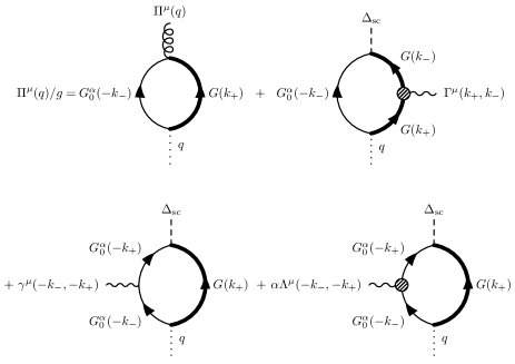
Figure 2: Self consistent equation for the collective modes after performing all possible vertex insertions into the gap equation.

Mathematically, Fig. (2) implies that the collective mode vertices must satisfy the following equation

$$\Pi^{\mu}(q)/g =\Pi^{\mu}(q)\sum_{k}G_{0}^{\alpha}(-k_{-})G(k_{+})$$

$$+\Delta_{\mathrm{sc}}\sum_{k}G_{0}^{\alpha}(-k_{-})G(k_{+})\Gamma^{\mu}(k_{+},k_{-})G(k_{-})$$

$$+\Delta_{\mathrm{sc}}\sum_{k}\biggl{(}G_{0}^{\alpha}(-k_{-})G_{0}^{\alpha}(-k_{+})G(k_{+})$$

$$\quad\quad\quad\times\left[\gamma^{\mu}(k_{+},k_{-})+\Lambda^{\mu}(k_{+},k_{-})\right]\biggr{)}.$$ (2.9)

Notice that the full vertex $\Gamma^{\mu}(k_{+},k_{-})$ appears in this expression. The full vertex was already determined in Eq. (II.2) using the Ward-Takahashi identity. Therefore if we insert the expression for the full vertex, which contains the collective mode vertices, into Eq. (II.3) (and its conjugate), then Eq. (II.3) (and its conjugate) becomes a self-consistent set of equations for the collective mode vertices $\Pi^{\mu}$ and $\bar{\Pi}^{\mu}$. The solution to this self-consistent set of linear equations will uniquely determine the collective mode vertices.

Inserting the full vertex into Eq. (II.3), and doing the same analysis for the conjugate gap equation, then gives the following two self-consistent equations for the collective mode vertices

$$\Pi^{\mu}(q)/g =\Pi^{\mu}(q)\sum_{k}G(k_{+})G^{\alpha}_{0}(-k_{-})\left[1-\Delta_{\mathrm{sc}}^{*}F_{\mathrm{sc}}(k_{-})\right]$$

$$-\bar{\Pi}^{\mu}(q)\sum_{k}F_{\mathrm{sc}}(k_{+})F_{\mathrm{sc}}(k_{-})$$

$$+\sum_{k}\left[\gamma^{\mu}(k_{+},k_{-})+\Lambda^{\mu}(k_{+},k_{-})\right]G(k_{+})F_{\mathrm{sc}}(k_{-})$$

$$+\sum_{k}\biggl{(}\left[\gamma^{\mu}(-k_{-},-k_{+})+\alpha\Lambda^{\mu}(-k_{-},-k_{+})\right]$$

$$\quad\times F_{\mathrm{sc}}(k_{+})G^{\alpha}_{0}(-k_{-})\left[1-\Delta^{*}_{\mathrm{sc}}F_{\mathrm{sc}}(k_{-})\right]\biggr{)},$$ (2.10)

$$\bar{\Pi}^{\mu}(q)/g =\bar{\Pi}^{\mu}(q)\sum_{k}G(k_{-})G^{\alpha}_{0}(-k_{+})\left[1-\Delta_{\mathrm{sc}}F^{*}_{\mathrm{sc}}(k_{+})\right]$$

$$-\Pi^{\mu}(q)\sum_{k}F^{*}_{\mathrm{sc}}(k_{+})F^{*}_{\mathrm{sc}}(k_{-})$$

$$+\sum_{k}\left[\gamma^{\mu}(k_{+},k_{-})+\Lambda^{\mu}(k_{+},k_{-})\right]F^{*}_{\mathrm{sc}}(k_{+})G(k_{-})$$

$$+\sum_{k}\biggl{(}\left[\gamma^{\mu}(-k_{-},-k_{+})+\alpha\Lambda^{\mu}(-k_{-},-k_{+})\right]$$

$$\quad\times G^{\alpha}_{0}(-k_{+})F^{*}_{\mathrm{sc}}(k_{-})\left[1-\Delta_{\mathrm{sc}}F^{*}_{\mathrm{sc}}(k_{+})\right]\biggr{)}.$$ (2.11)

This is conveniently expressed as a matrix equation if we define the two-point correlation functions

$$Q_{+-}(q) =1/g-\sum_{k}G(k_{+})G^{\alpha}_{0}(-k_{-})\left[1-\Delta_{\mathrm{sc}}^{*}F_{\mathrm{sc}}(k_{-})\right],$$

$$Q_{++}(q) =\sum_{k}F_{\mathrm{sc}}(k_{+})F_{\mathrm{sc}}(k_{-}),$$

$$P^{\mu}_{+}(q) =\sum_{k}\left[\gamma^{\mu}(k_{+},k_{-})+\Lambda^{\mu}(k_{+},k_{-})\right]G(k_{+})F_{\mathrm{sc}}(k_{-})$$

$$+\sum_{k}\left[\gamma^{\mu}(-k_{-},-k_{+})+\alpha\Lambda^{\mu}(-k_{-},-k_{+})\right]\times$$

$$\quad F_{\mathrm{sc}}(k_{+})G^{\alpha}_{0}(-k_{-})\left[1-\Delta^{*}_{\mathrm{sc}}F_{\mathrm{sc}}(k_{-})\right],$$ (2.12)

and $Q_{-+}(q)=Q_{+-}^{*}(q)$, $Q_{--}(q)=Q_{++}^{*}(q)$, $\Delta_{\mathrm{sc}}^{*}P^{\mu}_{+}(q)=\Delta_{\mathrm{sc}}P^{\mu}_{-}(-q)$. To connect to the literature, we define an alternative set of of two-point correlation functions $Q_{ab}$ and $Q^{a\mu}$, where $a,b=1,2$ through, $Q_{11}=Q_{+-}+Q_{-+}+Q_{++}+Q_{--},$ $Q_{22}=Q_{+-}+Q_{-+}-Q_{++}-Q_{--},$ $Q_{12}=i(Q_{+-}-Q_{-+}+Q_{--}-Q_{++}),$ $Q_{21}=-i(Q_{+-}-Q_{-+}+Q_{++}-Q_{--})$, and $Q^{1\mu}=-\left(P^{\mu}_{+}+P^{\mu}_{-}\right)$, $Q^{2\mu}=-i(P^{\mu}_{-}-P^{\mu}_{+})$. Similarly, we define the collective mode vertices $\Pi^{\mu}_{1,2}(q)$ through $\Pi^{\mu}(q)=\Pi^{\mu}_{1}(q)+i\Pi^{\mu}_{2}(q)$, $\bar{\Pi}^{\mu}(q)=\Pi^{\mu}_{1}(q)-i\Pi^{\mu}_{2}(q)$. This amounts to a change of basis from a complex to a real and imaginary parameterization. From Eq. (II.3) and Eq. (2.11), these vertices satisfy the relation

$$\left(\begin{array}[]{c}\Pi^{\mu}_{1}\\ \Pi^{\mu}_{2}\end{array}\right)=-\left(\begin{array}[]{cc}Q_{11}&Q_{12}\\ Q_{21}&Q_{22}\end{array}\right)^{-1}\left(\begin{array}[]{c}Q^{1\mu}\\ Q^{2\mu}\end{array}\right).$$ (2.13)

The form of these collective mode vertices is structurally similar to the BCS case Hao1 ; Hao2 , and in the strict BCS limit they agree with the literature Hao1 . The matrix $Q_{ab}$ can be interpreted as a propagator for bosonic degrees of freedom. However, the explicit response functions entering on the right hand side of Eq. (2.13) are modified due to the presence of the self-energy $\Sigma_{\mathrm{corr}}$.

In the Supplemental Material Supplement we verify that the collective mode vertices $\Pi^{\mu}(q)$ and $\bar{\Pi}^{\mu}(q)$ satisfy the gauge invariant conditions $q_{\mu}\Pi^{\mu}(q)=2\Delta_{\mathrm{sc}}$, $q_{\mu}\bar{\Pi}^{\mu}(q)=-2\Delta_{\mathrm{sc}}^{*}$, which was assumed in their definitions.

II.4 Vertex correction $\Lambda^{\mu}$

We can now summarize the central results of this paper, and repeat key equations. The full electromagnetic response kernel can generically be written as

$$K^{\mu\nu}(q) =2\sum_{k}G(k_{+})\Gamma^{\mu}(k_{+},k_{-})G(k_{-})\gamma^{\nu}(k_{-},k_{+})$$

$$\quad+\frac{n}{m}\delta^{\mu\nu}(1-\delta_{0\mu}),$$ (II.1)

where the full vertex

$$\Gamma^{\mu} (k_{+},k_{-})=\gamma^{\mu}(k_{+},k_{-})+\Lambda^{\mu}(k_{+},k_{-})$$

$$-\Delta_{\mathrm{sc}}^{*}\Pi^{\mu}(q)G^{\alpha}_{0}(-k_{-})-\Delta_{\mathrm{sc}}\bar{\Pi}^{\mu}(q)G^{\alpha}_{0}(-k_{+})$$

$$-|\Delta_{\mathrm{sc}}|^{2}G^{\alpha}_{0}(-k_{-})G^{\alpha}_{0}(-k_{+})\times$$

$$\quad[\gamma^{\mu}(-k_{-},-k_{+})+\alpha\Lambda^{\mu}(-k_{-},-k_{+})],$$ (II.2)

contains contributions due to both the collective mode vertices $\Pi^{\mu}$ and $\bar{\Pi}^{\mu}$ (computed in Eq. (2.13)) and the vertex contribution $\Lambda^{\mu}$ arising from the self-energy $\Sigma_{\mathrm{corr}}$.

The techniques described above are sufficient to calculate a gauge invariant response function for a large class of theories. All that is required to derive the full gauge invariant electromagnetic response is to arrive at a form of $\Lambda^{\mu}$. This vertex depends on the details of the correlation self-energy $\Sigma_{\mathrm{corr}}$, so we must consider it on a case by case basis. We now consider three relevant examples from the literature.

II.4.1 Pairing pseudogap

The first type of strong correlations we study is that proposed in Ref. Norman at a phenomenological level and in Ref. ourreview from a more microscopic perspective. In Ref. Kosztin an early attempt to address how collective modes are affected by these pseudogap effects was performed. This model is based on a BCS like self-energy but with a normal state gap $\Delta_{\mathrm{pg}}$. For this model, which we call the “pairing pseudogap approximation”, $\alpha=0$ in Eq. (2.3), and the correlated self-energy in Eq. (2.5) is given by

$$\Sigma_{\mathrm{corr}}(k)=-\Delta_{\mathrm{pg}}^{2}G_{0}(-k).$$ (2.14)

The pairing gap $\Delta_{\mathrm{pg}}$ is non-zero in the range of temperatures $T^{*}>T_{c}>0$, where $T^{*}$ is the mean-field transition temperature ($\Delta_{\mathrm{pg}}(T^{*}=0$)). At a more microscopic level ourreview $\Delta_{\mathrm{pg}}$ is to be associated with non-condensed (finite momentum) pairs and is distinct from the superconducting order parameter $\Delta_{\mathrm{sc}}$ which corresponds to a condensate of pairs at zero net momentum.

Unlike the order parameter $\Delta_{\mathrm{sc}}$, the gap $\Delta_{\mathrm{pg}}$ does not fluctuate in the presence of $A_{\mu}$. Nevertheless, its inclusion in the self-energy will lead to a vertex correction. Using this form of $\Sigma_{\mathrm{corr}}(k)$, along with the definition $q_{\mu}\Lambda^{\mu}(k_{+},k_{-})=\Sigma_{\mathrm{corr}}(k_{-})-\Sigma_{\mathrm{corr}}(k_{+})$, we obtain

$$\Lambda^{\mu}(k_{+},k_{-})=\Delta_{\mathrm{pg}}^{2}G_{0}(-k_{-})\gamma^{\mu}(-k_{-},-k_{+})G_{0}(-k_{+}).$$ (2.15)

Inserting this expression into Eq. (II.2), along with $\alpha=0$, then gives the full superconducting vertex in the pseudogap approximation.

Note that the pseudogap self-energy is an approximation of a theory with $\alpha=0$ and $\Sigma_{\mathrm{corr}}(k)=\sum_{l}t_{\mathrm{pg}}(l)G_{0}(l-k)$, where $t_{\mathrm{pg}}(l)$ is a $t$-matrix. This theory was considered in Ref. Hao2 , and the vertex $\Lambda^{\mu}$ was calculated exactly. The exact $t_{\mathrm{pg}}$ depends on the full Green’s function, so the exact $\Lambda^{\mu}$ will itself depend on the full vertex $\Gamma^{\mu}$, and thus a self-consistent integral equation will arise for $\Gamma^{\mu}$. In the pairing pseudogap approximation, $\Delta_{\mathrm{pg}}$ is constructed such that it contains no external momentum. Thus no vertex insertions into the gap are possible in $\Lambda^{\mu}$, resulting in the above condition that $\Delta_{\mathrm{pg}}$ does not fluctuate with $A_{\mu}$.

II.4.2 YRZ model

As a second model we consider a phenomenological self-energy developed for the high-$T_{c}$ superconductors and associated with Yang, Rice, and Zhang YRZ . This is known as the YRZ model. For the YRZ model, in Eq. (2.3) and Eq. (2.5) one sets $\alpha=1$ and

$$\Sigma_{\mathrm{corr}}(k)=-\Delta_{\mathrm{pg}}^{2}G_{0}(-k).$$ (2.16)

Since $\Sigma_{\mathrm{corr}}(k)$ is the same as in the pairing pseudogap approximation, in the YRZ model we also obtain

$$\Lambda^{\mu}(k_{+},k_{-})=\Delta_{\mathrm{pg}}^{2}G_{0}(-k_{-})\gamma^{\mu}(-k_{-},-k_{+})G_{0}(-k_{+}).$$ (2.17)

Inserting this vertex correction into Eq. (II.2), along with $\alpha=1$, then gives the full superconducting vertex in the YRZ model. In the normal state, this full vertex, along with the response kernel in Eq. (II.1), is in agreement with the results obtained in Ref. Peter1 . Here we have extended this work to the superconducting case.

II.4.3 Particle-only $t$-matrix

A third and final model was introduced by Strinati and co-workers using a generalized $t$-matrix StrinatiPRL ; StrinatiPRB ; StrinatiPRB2 . In this model the self-energy is obtained from Eq. (2.3) and Eq. (2.5) by setting $\alpha=1$ and

$$\Sigma_{\mathrm{corr}}(k)=\sum_{l}t(l)G_{\mathrm{BCS}}(l-k).$$ (2.18)

Here $G_{\mathrm{BCS}}$ is the full Green’s function as would be defined in a pure BCS theory; $t(l)$ is a $t$-matrix, the details of which are presented in the Supplemental Material Supplement . In Ref. StrinatiPRB2 , the authors propose “good candidates” for the response function Feynman diagrams. Here we emphasize that the WTI provides a direct procedure to determine not just good candidates but the exact full vertex, given in Eq. (II.2), which is manifestly gauge invariant. The challenge here is in determining the exact vertex correction $\Lambda^{\mu}(k_{+},k_{-})$. This is more complicated than in the previous two cases. Nevertheless, following the procedure outlined above, the vertex correction due to this self-energy can be obtained by performing all possible vertex insertions into all internal lines. That is, by inserting all possible vertices into both the Green’s function and into the $t$-matrix. In the Supplemental Material Supplement we explicitly derive the vertex correction $\Lambda^{\mu}$ for the self-energy appearing in Eq. (2.18). We should note that the authors of this body of work do not presume a self-consistent gap equation, such as that appearing in Eq. (2.6), and such as we have assumed in arriving at Eq. (2.13). Rather, they fix the order parameter to be the same as in BCS theory.

In summary, this section has shown how to derive a gauge invariant full vertex for a generic self-energy of the form in Eq. (2.5). Using the Ward-Takahashi identity there is an exact procedure to determine the full vertex. Moreover there is an analogous procedure to determine the collective modes and thus maintain gauge invariance. The resulting Feynman diagrams, which are shown in the Supplemental Material Supplement , are then completely determined.

III Alternative scheme to Ward-Takahashi: Path Integral

III.1 Gauge invariant electrodynamics

A large class of theories in the literature derive the gauge invariant electromagnetic response using a path integral approach Altland ; Kitagawa ; Yakovenko . We now connect, when possible, the above results using the Ward-Takahashi identity to the EM response as calculated in the path integral literature. Here we will include both amplitude and phase fluctuations of the order parameter Taylor ; Randeria1 . This is in contrast to previous studies Altland ; Kitagawa ; Yakovenko which incorporate only phase fluctuations. We introduce these amplitude fluctuations in large part in order to address the compressibility sum-rule.

The inverse Nambu Green’s function is $\mathcal{G}^{-1}=\mathcal{G}^{-1}_{0}-\Sigma$, where $\mathcal{G}_{0}^{-1}=i\omega-\xi_{\mathbf{k}}\tau_{3}$ and the self-energy is $\Sigma=-\Delta(x)\tau_{+}-\Delta^{*}(x)\tau_{-}$. The Nambu Pauli matrices are $\tau_{1,2,3}$, which define the raising and lowering operators $\tau_{\pm}=\frac{1}{2}\left(\tau_{1}\pm i\tau_{2}\right)$. We begin with the action functional in terms of the Hubbard-Stratonovich field $\Delta$ Taylor :

$$S[\Delta^{*},\Delta,A^{\mu}]=-\mathrm{Tr\ ln}\left[-\mathcal{G}^{-1}\right]+\int dx\ \frac{|\Delta(x)|^{2}}{g},$$ (3.1)

and following convention, the trace Tr represents a trace over both Nambu and position indices. We now follow the literature and perform the saddle point expansion. To lowest order the effective action is $S_{\mathrm{eff}}[\Delta^{*},\Delta,A^{\mu}]=S_{\mathrm{mf}}[\Delta_{\mathrm{mf}}^{*},\Delta_{\mathrm{mf}}]$, where the mean-field (mf) action is

$$S_{\mathrm{mf}}[\Delta_{\mathrm{mf}}^{*},\Delta_{\mathrm{mf}}]=-\mathrm{Tr}\ \mathrm{ln}\left[-\mathcal{G}_{\mathrm{mf}}^{-1}\right]+\int dx\ \frac{|\Delta_{\mathrm{mf}}|^{2}}{g},$$ (3.2)

and the inverse mean-field Nambu Green’s function is $\mathcal{G}^{-1}_{\mathrm{mf}}=\mathcal{G}^{-1}_{0}-\Sigma[\Delta(x)\rightarrow\Delta_{\mathrm{mf}}]$. The BCS gap equation then follows upon setting $\delta S_{\mathrm{mf}}[\Delta_{\mathrm{mf}}^{*},\Delta_{\mathrm{mf}}]/\delta\Delta_{\mathrm{mf}}^{*}=0$. It is straightforward to see that the resulting response kernel is not gauge invariant.

We now calculate the gauge invariant EM response kernel $K^{\mu\nu}$. In order to implement gauge invariance, the conventional literature introduces fluctuations $\eta(x)$ about the mean-field value of the order parameter $\Delta_{\mathrm{mf}}$, expressing $\Delta(x)=\Delta_{\mathrm{mf}}+\eta(x)$. (In Sec. (II), $\Delta_{\mathrm{sc}}\equiv\Delta_{\mathrm{mf}}$ for strict BCS theory.) Expanding the action functional to second order in $\eta(x)$ gives $S[\Delta^{*},\Delta,A^{\mu}]\approx S_{\mathrm{mf}}[\Delta_{\mathrm{mf}}^{*},\Delta_{\mathrm{mf}}]+S^{(2)}[\eta^{*},\eta,A^{\mu}]$. To calculate $S^{(2)}[\eta^{*},\eta,A^{\mu}]$, we first consider fluctuations of the Green’s function about the mean-field solution:

$$\mathcal{G}^{-1}-\mathcal{G}^{-1}_{\mathrm{mf}}=-\delta\Gamma-\Sigma_{\eta},$$ (3.3)

where $\delta\Gamma=\Gamma_{1}+\Gamma_{2}$, with $\Gamma_{1}=\gamma_{\mu}A^{\mu}$, $\Gamma_{2}=(\mathbf{A}^{2}/2m)\tau_{3}$, is a vector potential fluctuation and $\Sigma_{\eta}=\Sigma[\Delta(x)\rightarrow\eta(x)]$ is a gap fluctuation. Expanding to second order in $\eta$ and $A_{\mu}$, the second order action functional is

$$S^{(2)}[\eta^{*},\eta,A^{\mu}]$$

$$=\frac{1}{2}\sum_{q}\left[A_{\mu}(q)K^{\mu\nu}_{0,\mathrm{mf}}(q)A_{\nu}(-q)+\eta_{a}(q)Q^{ab}_{\mathrm{mf}}(q)\eta_{b}(-q)\right]$$

$$+\frac{1}{2}\sum_{q}\left[A_{\mu}(q)Q^{\mu b}_{\mathrm{mf}}(q)\eta_{b}(-q)+\eta_{a}(q)Q^{a\nu}_{\mathrm{mf}}(q)A_{\nu}(-q)\right].$$

In this expression we write $\eta(x)=\eta_{1}(x)-i\eta_{2}(x)$ with $\eta_{1}(x),\eta_{2}(x)\in\mathbb{R}$. This decomposes the fluctuations into their (Cartesian) real and imaginary parts, which amounts to an amplitude and phase decomposition. Since we keep the saddle point condition at the mean-field level, an explicit amplitude and phase decomposition, in polar coordinates, will lead to the same electromagnetic response. (If one uses a different saddle point condition, not relevant to this work, then issues associated with the use of either a Cartesian or polar decomposition may arise Randeria1 .) Even within this framework, we shall point out an inconsistency within the conventional path integral formalism in failing to satisfy the compressibility sum-rule.

To complete the calculation, we transform to momentum space, $k=(i\omega_{n},\mathbf{k})$ and $q=(i\Omega_{m},\mathbf{q})$, where $i\omega_{n}$ $(i\Omega_{m})$ is a fermionic (bosonic) Matsubara frequency. If we denote the trace over Nambu indices by tr, then the “bubble” response kernel is $K^{\mu\nu}_{0,\mathrm{mf}}(q)=\mathrm{tr}\sum_{k}\mathcal{G}_{\mathrm{mf}}(k_{+})\gamma^{\mu}(k_{+},k_{-})\mathcal{G}_{\mathrm{mf}}(k_{-})\gamma^{\nu}(k_{-},k_{+})+\tfrac{n}{m}\delta^{\mu\nu}(1-\delta_{\mu 0})$ and the two-point response function $Q^{ab}_{\mathrm{mf}}(q)=\tfrac{2}{g}\delta_{ab}+\mathrm{tr}\sum_{k}\mathcal{G}_{\mathrm{mf}}(k_{+})\tau_{a}\mathcal{G}_{\mathrm{mf}}(k_{-})\tau_{b}$ can be viewed as a bosonic propagator. We also have $Q^{\mu a}_{\mathrm{mf}}(q)=-\mathrm{tr}\sum_{k}\mathcal{G}_{\mathrm{mf}}(k_{+})\gamma^{\mu}(k_{+},k_{-})\mathcal{G}_{\mathrm{mf}}(k_{-})\tau_{a}$, and $Q^{b\nu}_{\mathrm{mf}}(q)$ has $(\mu,a)\leftrightarrow(b,\nu)$. These mean-field response functions are equivalent to previous results in the literature Hao1 . They are also equivalent to the response functions which appear in Eq. (2.13) for a theory with only a strict BCS self-energy.

After integrating out the $\eta$ field, the beyond-mean-field effective action contribution is given by

$$S_{\mathrm{eff}}-S_{\mathrm{mf}} =\sum_{q}A_{\mu}(q)K^{\mu\nu}_{\mathrm{mf}}(q)A_{\nu}(-q)$$

$$\quad+\frac{1}{2}\mathrm{Tr}\ \mathrm{ln}\left[Q^{ab}_{\mathrm{mf}}(q)\right].$$ (3.4)

Thus the fluctuation action decomposes into two separate terms. The second term in the fluctuation action provides a contribution to thermodynamics arising from Gaussian fluctuations. This form of the Gaussian fluctuation part of the action is equivalent to the standard results in the literature Randeria1 . The first term is the gauge invariant EM response kernel, with both amplitude and phase fluctuations of the order parameter included, defined by $K^{\mu\nu}_{\mathrm{mf}}(q)=K^{\mu\nu}_{0,\mathrm{mf}}(q)-\sum_{a,b}Q^{\mu a}_{\mathrm{mf}}(q)\left[Q^{ab}_{\mathrm{mf}}(q)\right]^{-1}Q^{b\nu}_{\mathrm{mf}}(-q)$. If we expand the response kernel appearing in Eq. (III.1), then we obtain Hao1 ; Kulik :

$$K^{\mu\nu}_{\mathrm{mf}}=K^{\mu\nu}_{0,\mathrm{mf}}-\frac{Q_{11}Q^{\mu 2}_{\mathrm{mf}}Q^{2\nu}_{\mathrm{mf}}+Q_{22}Q^{\mu 1}_{\mathrm{mf}}Q^{1\nu}_{\mathrm{mf}}-Q_{12}Q^{\mu 1}_{\mathrm{mf}}Q^{2\nu}_{\mathrm{mf}}-Q_{21}Q^{\mu 2}_{\mathrm{mf}}Q^{1\nu}_{\mathrm{mf}}}{Q_{11}Q_{22}-Q_{12}Q_{21}}.$$ (3.5)

In Ref. Hao1 it is proved that the response kernel in Eq. (3.5) is both gauge invariant $q_{\mu}K^{\mu\nu}_{\mathrm{mf}}(q)=0$, and charge conserving $K^{\mu\nu}_{\mathrm{mf}}(q)q_{\nu}=0$. References Hao1 ; Kulik used a matrix linear response formalism known as “consistent fluctuation of the order parameter”. Our derivation, however, is based on the path integral.

III.2 Inconsistency with the compressibility sum-rule

We now turn to the implications of the two contributions to the action in Eq. (III.1). Here we focus on the compressibility sum-rule, which provides an important consistency check on the path integral approach. The explicit form of the compressibility sum-rule is Pines :

$$\mathrm{lim}_{\mathbf{q}\rightarrow 0}\left[K^{00}(\omega=0,\mathbf{q})\right]=-\frac{\partial n}{\partial\mu}.$$ (3.6)

This sum-rule shows how to associate the electromagnetic contributions to the action with their counterpart contributions to the thermodynamic response.

The compressibility, $\kappa=n^{-2}(\partial n/\partial\mu)$, is then related to the density response via Eq. (3.6). Here the real frequency $\omega$ is the analytic continuation of the Matsubara frequency $i\Omega$, defined by $i\Omega=\omega+i\gamma$ with $\gamma\rightarrow 0$. The relationship in Eq. (3.6) is particularly useful in characterizing various orders of approximation within the path integral scheme. This is because at the heart of the path integral is a close connection between electrodynamics and thermodynamics. With the inclusion of amplitude fluctuations, which are essential for this sum-rule, we can now test the compressibility sum-rule within the standard path integral formalism in the literature.

Note that, this sum-rule depends on the number equation. Consistency would seem to require that we include Gaussian fluctuations $n_{\mathrm{fl}}=-\beta^{-1}\partial S_{\mathrm{fl}}[\Delta_{\mathrm{mf}}^{*},\Delta_{\mathrm{mf}}]/\partial\mu$ to the number equation coming from the second line in Eq. (III.1). This is, in fact, incorrect and points to an underlying inconsistency. Instead, we will show the proper calculation level for thermodynamics is that of pure mean-field, giving a mean-field particle number

$$n_{\mathrm{mf}}=-\frac{1}{\beta}\frac{\partial S_{\mathrm{mf}}[\Delta_{\mathrm{mf}}^{*},\Delta_{\mathrm{mf}}]}{\partial\mu}=2\sum_{k}G(k).$$ (3.7)

Taking the derivative of the mean-field number equation with respect to $\mu$ gives

$$\frac{\partial n_{\mathrm{mf}}}{\partial\mu}=-2\sum_{k}\left[G^{2}(k)-F^{2}(k)+2G(k)F(k)\frac{\partial\Delta_{\mathrm{mf}}}{\partial\mu}\right],$$ (3.8)

where we henceforth take $\Delta_{\mathrm{mf}}=\Delta_{\mathrm{mf}}^{*}$ for convenience. Here we define the single particle Green’s function in terms of the Nambu Green’s function by $G(k)=(\mathcal{G}_{\mathrm{mf}}(k))_{11}=-(\mathcal{G}_{\mathrm{mf}}(-k))_{22}$, and the anomalous Green’s function is similarly $F(k)=\Delta_{\mathrm{mf}}G(k)G_{0}(-k)=(\mathcal{G}_{\mathrm{mf}}(k))_{12}=(\mathcal{G}^{*}_{\mathrm{mf}}(k))_{21}$. The fluctuation of the mean-field gap with respect to the chemical potential, $\partial\Delta_{\mathrm{mf}}/\partial\mu$, can be found using the BCS gap equation

$$\mathrm{GAP}[\Delta_{\mathrm{mf}},\mu]:=\frac{\Delta_{\mathrm{mf}}}{g}-\sum_{k}\mathrm{Tr}[\mathcal{G}(k)\tau_{-}]=0.$$ (3.9)

Since $\Delta_{\mathrm{mf}}$ depends on $\mu$, by taking the total derivative with respect to $\mu$, we arrive at the condition

$$\frac{\partial\Delta_{\mathrm{mf}}}{\partial\mu}=-\frac{\partial\mathrm{GAP}/\partial\mu}{\partial\mathrm{GAP}/\partial\Delta_{\mathrm{mf}}}.$$ (3.10)

To see that the compressibility sum-rule is satisfied, notice that $\partial\mathrm{GAP}/\partial\mu=2\sum_{k}G(k)F(k)$ and $\partial\mathrm{GAP}/\partial\Delta=2\sum_{k}F(k)F(k)$. Therefore, the last term in Eq. (3.8) can be expressed as $2\frac{\left(\partial\mathrm{GAP}/\partial\mu\right)^{2}}{\partial\mathrm{GAP}/\partial\Delta_{\mathrm{mf}}}$. Now, in the limit that $\omega=0,\mathbf{q}\rightarrow 0$, the following identifications can be made: $Q^{10}_{\mathrm{mf}}=2\partial\mathrm{GAP}/\partial\mu$, and $Q^{11}_{\mathrm{mf}}=2\partial\mathrm{GAP}/\partial\Delta_{\mathrm{mf}}$. By computing the summation over Matsubara frequencies, one also obtains $2\sum_{k}\left[G^{2}(k)-F^{2}(k)\right]=K^{00}_{0,\mathrm{mf}}$.

Therefore, using Eq. (3.5), Eq. (3.8) now becomes

$$-\frac{\partial n_{\mathrm{mf}}}{\partial\mu}=K^{00}_{0,\mathrm{mf}}-\frac{Q^{10}_{\mathrm{mf}}Q^{01}_{\mathrm{mf}}}{Q_{11}}=K^{00}(0,\mathbf{q}\rightarrow 0).$$ (3.11)

This demonstrates the expected consistency between $-(\partial n_{\mathrm{mf}}/\partial\mu)$ and $K^{00}(0,\mathbf{q}\rightarrow 0)$ and proves the compressibility sum-rule at the BCS level Hao1 .

The reason for the need to include amplitude fluctuations in the density-density response can be seen from Eq. (3.8). This equation shows that fluctuations in the gap ($\partial\Delta_{\mathrm{mf}}/\partial\mu$) must be included, and therefore amplitude fluctuations in the gap are necessary in order to satisfy the compressibility sum-rule. If only phase fluctuations are retained, the compressibility sum-rule is violated. For a different context where amplitude fluctuations are important see Ref. Salasnich .

The compressibility sum-rule has only been satisfied by ignoring the Gaussian fluctuations in the number equation. Had these been included, we would obtain $-\partial n/\partial\mu=-\partial n_{\mathrm{mf}}/\partial\mu-\partial n_{\mathrm{fl}}/\partial\mu\neq K^{00}(0,\mathbf{q}\rightarrow 0),$ which violates the compressibility sum-rule.

In summary, the path integral formalism, as currently applied in the literature, treats electrodynamics and thermodynamics inconsistently. In this derivation of gauge invariant electrodynamics at the BCS level, beyond BCS fluctuations are necessarily incorporated in thermodynamics. However, these thermodynamic fluctuations should not appear in the number equation if the compressibility sum rule is to be satisfied. The discussion in Sec. (II) provides insights into the resolution to this inconsistency: there gauge invariance is obtained by determining the collective modes that arise due to vertex insertions into the gap equation. This suggests that, within the path integral formalism, one should consider a new saddle point condition in the presence of a non-zero vector potential. More details on this resolution are presented elsewhere ourcompanion .

IV Conclusions

The goal of this paper was to show how to arrive at a proper gauge invariant description of the electromagnetic response in strongly correlated fermionic superfluids. In this paper correlation effects are represented by “correlated self-energy” contributions which appear in addition to the usual BCS self-energy of the condensate. Using the Ward-Takahashi identity, and adopting a rather generic class of such models (widely used for the high temperature superconductors and ultra cold gases) we are able to give exact expressions for the electromagnetic response. The results appear in a closed form as a consequence of the fact that the correlation self-energy depends on only bare or partially dressed Green’s functions. Our method, which obtains expressions for all vertex corrections and collective modes in a manner compatible with the $f$-sum-rule, is an important tool for studying strongly correlated superfluids and superconductors.

For comparison we also discuss an alternative tool which builds on the path integral approach. With few exceptions this scheme has been used to address the BCS-level response, i.e., in the absence of stronger correlations. In contrast to approaches which build on the Ward-Takahashi identity, here gauge invariance and the $f$-sum-rule are relatively straightforward to ensure. What is more complicated is to arrive at consistency with the compressibility sum-rule. This sum-rule relates electrodynamics and thermodynamics and provides a natural test of the path integral scheme, since the two are simultaneously calculated. We show that in the conventional path integral literature for the gauge invariant electrodynamics at the BCS level, the compressibility sum-rule is violated.

Acknowledgements.$-$ This work was supported by NSF-DMR-MRSEC 1420709. We are particularly grateful to Hao Guo and Yan He for sharing their insights and for sending us their preprints on a related topic.

See pages 1 of Supplement_arxiv_resubmit.pdf See pages 2 of Supplement_arxiv_resubmit.pdf See pages 3 of Supplement_arxiv_resubmit.pdf See pages 4 of Supplement_arxiv_resubmit.pdf See pages 5 of Supplement_arxiv_resubmit.pdf See pages 6 of Supplement_arxiv_resubmit.pdf See pages 7 of Supplement_arxiv_resubmit.pdf

References

- (1) E. Taylor, A. Griffin, N. Fukushima, and Y. Ohashi, Phys. Rev. A 74, 063626 (Dec 2006), http://link.aps.org/doi/10.1103/PhysRevA.74.063626
- (2) R. B. Diener, R. Sensarma, and M. Randeria, Phys. Rev. A 77, 023626 (Feb 2008), http://link.aps.org/doi/10.1103/PhysRevA.77.023626
- (3) K.-Y. Yang, T. M. Rice, and F.-C. Zhang, Phys. Rev. B 73, 174501 (May 2006), http://link.aps.org/doi/10.1103/PhysRevB.73.174501
- (4) P. A. Lee, Phys. Rev. X 4, 031017 (Jul 2014), http://link.aps.org/doi/10.1103/PhysRevX.4.031017
- (5) M. R. Norman, M. Randeria, H. Ding, and J. C. Campuzano, Phys. Rev. B 57, R11093 (May 1998), http://link.aps.org/doi/10.1103/PhysRevB.57.R11093
- (6) Q. Chen, J. Stajic, S. Tan, and K. Levin, Physics Reports 412, 1 (2005), ISSN 0370-1573, http://www.sciencedirect.com/science/article/pii/S0370157305001067
- (7) A. Altland and B. D. Simons, Condensed matter field theory (Cambridge University Press, 2010)
- (8) R. M. Lutchyn, P. Nagornykh, and V. M. Yakovenko, Phys. Rev. B 77, 144516 (Apr 2008), http://link.aps.org/doi/10.1103/PhysRevB.77.144516
- (9) T. Ojanen and T. Kitagawa, Phys. Rev. B 87, 014512 (Jan 2013), http://link.aps.org/doi/10.1103/PhysRevB.87.014512
- (10) Y. Nambu, Phys. Rev. 117, 648 (Feb 1960), http://link.aps.org/doi/10.1103/PhysRev.117.648
- (11) A. G. Loeser, Z.-X. Shen, D. S. Dessau, D. S. Marshall, C. H. Park, P. Fournier, and A. Kapitulnik, Science 273, 325 (1996), ISSN 0036-8075, http://science.sciencemag.org/content/273/5273/325
- (12) B. M. Anderson, R. Boyack, C.-T. Wu, and K. Levin, ArXiv e-prints(Feb. 2016), 1602.03525
- (13) G. Baym and L. P. Kadanoff, Phys. Rev. 124, 287 (Oct 1961), http://link.aps.org/doi/10.1103/PhysRev.124.287
- (14) G. Baym, Phys. Rev. 127, 1391 (Aug 1962), http://link.aps.org/doi/10.1103/PhysRev.127.1391
- (15) P. W. Anderson, Phys. Rev. 110, 827 (May 1958), http://link.aps.org/doi/10.1103/PhysRev.110.827
- (16) L. P. Kadanoff and P. C. Martin, Phys. Rev. 124, 670 (Nov 1961), http://link.aps.org/doi/10.1103/PhysRev.124.670
- (17) I. Kulik, O. Entin-Wohlman, and R. Orbach, Journal of Low Temperature Physics 43, 591 (1981), ISSN 0022-2291, http://dx.doi.org/10.1007/BF00115617
- (18) H. Guo, C.-C. Chien, and Y. He, Journal of Low Temperature Physics 172, 5, ISSN 0022-2291, http://dx.doi.org/10.1007/s10909-012-0853-7
- (19) G. Rickayzen, Phys. Rev. 115, 795 (Aug 1959), http://link.aps.org/doi/10.1103/PhysRev.115.795
- (20) L. H. Ryder, Quantum field theory, 2nd ed. (Cambridge University Press, 1996)
- (21) M. Greiter, Annals of Physics 319, 217 (2005), ISSN 0003-4916, http://www.sciencedirect.com/science/article/pii/S0003491605000515
- (22) S. Elitzur, Phys. Rev. D 12, 3978 (Dec 1975), http://link.aps.org/doi/10.1103/PhysRevD.12.3978
- (23) P. Scherpelz, A. Rançon, Y. He, and K. Levin, Phys. Rev. B 90, 060506 (Aug 2014), http://link.aps.org/doi/10.1103/PhysRevB.90.060506
- (24) R. Boyack, C.-T. Wu, P. Scherpelz, and K. Levin, Phys. Rev. B 90, 220513 (Dec 2014), http://link.aps.org/doi/10.1103/PhysRevB.90.220513
- (25) Y. He and H. Guo, ArXiv e-prints(May 2015), arXiv:1505.04080 [cond-mat.quant-gas]
- (26) A. Perali, P. Pieri, L. Pisani, and G. C. Strinati, Phys. Rev. Lett. 92, 220404 (Jun 2004), http://link.aps.org/doi/10.1103/PhysRevLett.92.220404
- (27) P. Pieri, L. Pisani, and G. C. Strinati, Phys. Rev. B 70, 094508 (Sep 2004), http://link.aps.org/doi/10.1103/PhysRevB.70.094508
- (28) N. Andrenacci, P. Pieri, and G. C. Strinati, Phys. Rev. B 68, 144507 (Oct 2003), http://link.aps.org/doi/10.1103/PhysRevB.68.144507
- (29) J. R. Schrieffer, Theory of superconductivity, 1st ed. (W.A. Benjamin, Inc., 1964)
- (30) R. Boyack, B. M. Anderson, C.-T. Wu, and K. Levin, “Supplemental material: Includes a derivation of the exact full vertex, verifies that the collective mode vertices are gauge invariant, and derives the -sum rule,” (2016)
- (31) P. Nozieres, Theory of interacting Fermi systems, Advanced book classics (Addison-Wesley, Reading, MA, 1964)
- (32) I. Kosztin, Q. Chen, Y.-J. Kao, and K. Levin, Phys. Rev. B 61, 11662 (May 2000), http://link.aps.org/doi/10.1103/PhysRevB.61.11662
- (33) D. Pines and P. Nozieres, The theory of quantum liquids: normal Fermi liquids, Vol. 1 (WA Benjamin, 1966)
- (34) L. Salasnich, P. A. Marchetti, and F. Toigo, Phys. Rev. A 88, 053612 (Nov 2013), http://link.aps.org/doi/10.1103/PhysRevA.88.053612