The low-mass end of the baryonic Tully-Fisher relation
Abstract
The scaling of disk galaxy rotation velocity with baryonic mass (the “Baryonic Tully-Fisher” relation; BTF) has long confounded galaxy formation models. It is steeper than the scaling relating halo virial masses and circular velocities and its zero point implies that galaxies comprise a very small fraction of available baryons. Such low galaxy formation efficiencies may in principle be explained by winds driven by evolving stars, but the tightness of the BTF relation argues against the substantial scatter expected from such vigorous feedback mechanism. We use the APOSTLE/EAGLE simulations to show that the BTF relation is well reproduced in CDM simulations that match the size and number of galaxies as a function of stellar mass. In such models, galaxy rotation velocities are proportional to halo virial velocity and the steep velocity-mass dependence results from the decline in galaxy formation efficiency with decreasing halo mass needed to reconcile the CDM halo mass function with the galaxy luminosity function. Despite the strong feedback, the scatter in the simulated BTF is smaller than observed, even when considering all simulated galaxies and not just rotationally-supported ones. The simulations predict that the BTF should become increasingly steep at the faint end, although the velocity scatter at fixed mass should remain small. Observed galaxies with rotation speeds below km s-1 seem to deviate from this prediction. We discuss observational biases and modeling uncertainties that may help to explain this disagreement in the context of CDM models of dwarf galaxy formation.
keywords:
galaxies: structure, galaxies:haloes, galaxies: evolution1 Introduction
The empirical relation between the rotation velocity and luminosity of disk galaxies is not only a reliable secondary distance indicator (Tully & Fisher, 1977), but also provides important clues to the total mass and mass profiles of their host dark matter halos. The Tully-Fisher (TF) relation has now been extensively studied observationally; its dependence on photometric passband, in particular, is relatively well-understood, and the relation is now generally cast in terms of galaxy stellar mass rather than luminosity (e.g. McGaugh et al., 2000; Bell & de Jong, 2001; Pizagno et al., 2005; Torres-Flores et al., 2011).
This relation is well approximated by a single power law with small scatter, at least for late-type galaxies with stellar masses and velocities (McGaugh et al., 2000; Bell & de Jong, 2001). At lower masses/velocities, the relation deviates from a simple power law, presumably because the contribution of cold gas becomes more and more prevalent in dwarf galaxies. Indeed, the power-law scaling may be largely rectified at the faint end by considering baryonic masses rather than stellar mass alone. The “baryonic Tully-Fisher” relation, as this relation has become known (or BTF, for short), is well approximated by a single power law over roughly three decades in mass and a factor of six in velocity (McGaugh et al., 2000; Verheijen, 2001; Stark, McGaugh & Swaters, 2009). Its scatter is quite small, at least when only galaxies with high-quality data and radially-extended rotation curves are retained for analysis (McGaugh, 2012; Lelli, McGaugh & Schombert, 2016).
The interpretation of the Tully-Fisher relation in cosmologically-motivated models of galaxy formation has long been problematic. From a cosmological viewpoint, the Tully-Fisher relation is understood as reflecting the equivalence between halo mass and circular velocity imposed by the finite age of the Universe (see, e.g., Mo, Mao & White, 1998; Steinmetz & Navarro, 1999). That characteristic timescale translates into a fixed density contrast that implies a linear scaling between virial111We define the virial mass, , as that enclosed by a sphere of mean density times the critical density of the Universe, . Virial quantities are defined at that radius, and are identified by a “200” subscript. radius and velocity, or a simple relation between mass and circular velocity. A power-law scaling between galaxy mass and disk rotation velocity is therefore expected if galaxy mass and rotation speed scale with virial mass and virial velocity, respectively.
The latter conditions are not trivial to satisfy, as a simple example illustrates. The Milky Way’s baryonic mass is roughly (Rix & Bovy, 2013), and its rotation velocity is approximately constant at km/s over the whole Galactic disk, out to at least kpc. A halo of similar virial velocity, on the other hand, has a virial radius of kpc and a virial mass of order , or in baryons, assuming a cosmic baryon fraction of . A majority of these baryons can in principle cool and collapse into the Milky Way disk (see, e.g., White & Frenk, 1991). This example illustrates two important points: (i) only a small fraction of available baryons are today assembled at the center of the Milky Way halo, and (ii) the radius where disk rotational velocities are measured is much smaller than the virial radius of its surrounding halo, where its virial velocity is measured.
These points are quite important for models that try to account for the observed BTF relation. So few baryons assemble into galaxies that it is unclear how, or whether, their masses should scale with virial mass. Furthermore, the disk encompasses such a small fraction of the halo dark matter, and its kinematics probes the potential so far from the virial boundary, that a simple scaling between galaxy rotation speed and virial circular velocity might be justifiably discounted. Finally, it is quite conceivable that the mechanism that so effectively limits the fraction of baryons that settle into a galaxy (mainly feedback from evolving stars and supermassive black holes, in current models) might also exhibit large halo-to-halo variations due to the episodic nature of the star formation activity. This makes the rather tight scatter of the observed Tully-Fisher relation quite difficult to explain (McGaugh, 2012).
These difficulties explain why the literature is littered with failed attempts to reproduce the Tully-Fisher relation in a cold dark matter-dominated universe. Direct galaxy formation simulations, for example, have for many years consistently produced galaxies so massive and compact that their rotation curves were steeply declining and, generally, a poor match to observation (see, e.g., Navarro & Steinmetz, 2000; Abadi et al., 2003; Governato et al., 2004; Scannapieco et al., 2012, and references therein). Even semi-analytic models, where galaxy masses and sizes can be adjusted to match observation, have had difficulty reproducing the Tully-Fisher relation (see, e.g., Cole et al., 2000), typically predicting velocities at given mass that are significantly higher than observed unless somewhat arbitrary adjustments are made to the response of the dark halo (Dutton & van den Bosch, 2009).
The situation, however, has now started to change, notably as a result of improved recipes for the subgrid treatment of star formation and its associated feedback in direct simulations. As a result, recent simulations have shown that rotationally-supported disks with realistic surface density profiles and relatively flat rotation curves can actually form in cold dark matter halos when feedback is strong enough to effectively regulate ongoing star formation by limiting excessive gas accretion and removing low-angular momentum gas (see, e.g., Guedes et al., 2011; Brook et al., 2012; McCarthy et al., 2012; Aumer et al., 2013; Marinacci, Pakmor & Springel, 2014).
These results are encouraging but the number of individual systems simulated so far is small, and it is unclear whether the same codes would produce a realistic galaxy stellar mass function or reproduce the scatter of the Tully-Fisher relation when applied to a cosmologically significant volume. The role of the dark halo response to the assembly of the galaxy has remained particularly contentious, with some authors arguing that substantial modification to the innermost structure of the dark halo, in the form of a constant-density core or cusp expansion, is needed to explain the disk galaxy scaling relations (Dutton & van den Bosch, 2009; Chan et al., 2015), while other authors find no compelling need for such adjustment (see, e.g., Vogelsberger et al., 2014; Schaller et al., 2015b; Lacey et al., 2015).
The recent completion of ambitious simulation programmes such as the EAGLE project (Schaye et al., 2015; Crain et al., 2015), which follow the formation of thousands of galaxies in cosmological boxes Mpc on a side, allow for a reassessment of the situation. The subgrid physics modules of the EAGLE code have been calibrated to match the observed galaxy stellar mass function and the sizes of galaxies at , but no attempt has been made to match the BTF relation, which is therefore a true corollary of the model. The same is true of other relations, such as color bi-modality, morphological diversity, or the stellar-mass Tully-Fisher relation of bright galaxies, which are successfully reproduced in the model (Schaye et al., 2015; Trayford et al., 2015). Combining EAGLE with multiple realizations of smaller volumes chosen to resemble the surroundings of the Local Group of Galaxies (the APOSTLE project, see, e.g., Fattahi et al., 2016; Sawala et al., 2015), we are able to study the resulting BTF relation over four decades in galaxy mass. In particular, we are able to examine the simulation predictions for some of the faintest dwarfs, where recent data have highlighted potential deviations from a power-law BTF and/or increased scatter in the relation (Geha et al., 2006; Trachternach et al., 2009).
We begin with a brief description of EAGLE and APOSTLE in Sec. 2 and present our main results in Sec. 3. We investigate numerical convergence in Sec. 3.1. The gas/stellar content and size as a function of galaxy mass are presented in Sec. 3.2 before comparing the simulated BTF relation with observation in Sec. 3.3. We examine the predicted faint-end of the relation in Sec. 3.4 before concluding with a brief summary of our main conclusions in Sec. 4.
2 Numerical Simulations
2.1 The Code
The simulations we use here were run using a modified version of the SPH code P-Gadget 3 (Springel, 2005), as developed for the EAGLE simulation project (Schaye et al., 2015; Crain et al., 2015; Schaller et al., 2015a). We refer the reader to the main EAGLE papers for further details, but list here the main code features, for completeness. In brief, the code includes the “Anarchy” version of SPH (Dalla Vecchia, in preparation, see also Appendix A in Schaye et al. (2015)), which includes the pressure-entropy variant proposed by Hopkins (2013); metal-dependent radiative cooling/heating (Wiersma, Schaye & Smith, 2009), reionization of Hydrogen and Helium (at redshift and , respectively), star formation with a metallicity dependent density threshold (Schaye, 2004; Dalla Vecchia & Schaye, 2008), stellar evolution and metal production (Wiersma et al., 2009), stellar feedback via stochastic thermal energy injection (Dalla Vecchia & Schaye, 2012), and the growth of, and feedback from, supermassive black holes (Springel, Di Matteo & Hernquist, 2005; Booth & Schaye, 2009; Rosas-Guevara et al., 2015). The free parameters of the subgrid treatment of these mechanisms in the EAGLE code have been adjusted so as to provide a good match to the galaxy stellar mass function, the typical sizes of disk galaxies, and the stellar mass-black hole mass relation, all at .
2.2 The Simulations
We use two sets of simulations for the analysis we present here. One is the highest-resolution Mpc-box EAGLE run (Ref-L100N1504). This simulation has a cube side length of comoving Mpc; dark matter particles each of mass ; the same number of gas particles each of initial mass ; and a Plummer-equivalent gravitational softening length of proper pc (switching to comoving for redshifts higher than ). The cosmology adopted is that of Planck Collaboration et al. (2014), with , , , and .
The second set of simulations is the APOSTLE suite of zoom-in simulations, which evolve volumes tailored to match the spatial distribution and kinematics of galaxies in the Local Group (Fattahi et al., 2016). Each volume was chosen to contain a pair of halos with individual virial mass in the range -. The pairs are separated by a distance comparable to that between the Milky Way (MW) and Andromeda (M31) galaxies ( kpc) and approach with radial velocity consistent with that of the MW-M31 pair (- km/s).
The APOSTLE volumes were selected from the DOVE N-body simulation, which evolved a cosmological volume of Mpc on a side in the WMAP-7 cosmology (Komatsu et al., 2011). The APOSTLE runs were performed at three different numerical resolutions; low (AP-LR), medium (AP-MR) and high (AP-HR), differing by successive factors of in particle mass and in gravitational force resolution. All volumes have been run at medium and low resolutions, but only two high-res simulation volumes have been completed. Table 1 summarizes the main parameters of these simulations.
We use the SUBFIND algorithm to identify “galaxies”; i.e., self-bound structures (Springel et al., 2001; Dolag et al., 2009) in a catalog of friends-of-friends (FoF) halos (Davis et al., 1985) built with a linking length of times the mean interparticle separation. We retain for analysis only the central galaxy of each FoF halo, and remove from the analysis any system contaminated by lower-resolution particles in the APOSTLE runs. Baryonic galaxy masses (stellar plus gas) are computed within a fiducial “galaxy radius”, defined as . We have verified that this is a large enough radius to include the great majority of the star-forming cold gas and stars bound to each central galaxy.
| Particle Masses | Max Softening | |||
|---|---|---|---|---|
| Label | DM | Gas | [proper pc] | [] |
| AP-HR | ||||
| AP-MR | ||||
| AP-LR | ||||
| EAGLE | ||||
3 Results
3.1 Galaxy formation efficiency and numerical convergence
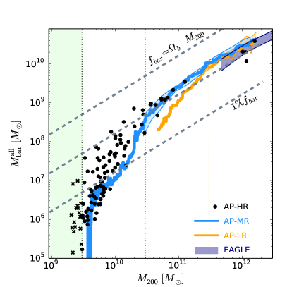
The left panel of Fig. 1 shows the relation between virial mass, , and galaxy baryonic mass, , in our simulations, where is computed by counting all gas and stellar particles within . Shaded regions bracket the interquartile range in as a function of virial mass for each of the simulation sets, as indicated in the legend. Thick solid lines of matching colors indicate the median trend. Individual symbols indicate results for the high-resolution AP-HR run, since the total number of galaxies in those two completed volumes is small.
The dashed grey lines indicate the location of galaxies whose masses make up (top), (middle) and of all baryons within the virial radius. Fig. 1 shows that the galaxy formation efficiency is low in all halos (less than ) and that it decreases steadily with decreasing virial mass. Galaxies in the most massive halos shown have been able to assemble roughly - of their baryons in the central galaxy, but the fraction drops to about in halos for the case of AP-HR. Such a steep decline is expected in any model that attempts to reconcile the shallow faint-end of the galaxy stellar mass function with the steep low-mass end of the halo mass function (see, e.g., the discussion in Sec. 5.2 of Schaye et al. 2015 and in Sec. of McCarthy et al. 2012).
The left panel of Fig. 1 also shows the limitations introduced by numerical resolution. The results for the various simulations agree for well-resolved halos, but the mean galaxy mass starts to deviate in halos resolved with small numbers of particles. This is most clearly appreciated when comparing the results of the median for each APOSTLE simulation set. AP-LR results, for example, “peel off” below the trend obtained in higher resolution runs for virial masses less than . Those from AP-MR, in turn, deviate from the AP-HR trend below . To define convergence for the high resolution run, we simply adopt a similar factor of between AP-MR and AP-HR. These limits are shown with thin vertical lines in the left panel of Fig. 1.
The issue of convergence in baryonic simulations is complex, since increasing resolution means that new physical processes enter into play and it is unclear whether a recalibration of the sub-grid physics should or should not be performed (see detailed discussion in Schaye et al., 2015). We adopt here the simple approach of selecting objects for which different resolutions give consistent baryonic masses. Noting that the particle mass (gas plus dark matter) is and for AP-LR and AP-HR, respectively, a simple rule of thumb is then that, on average, only halos resolved with at least particles give consistent galaxy masses for all runs. We highlight this mass range for each of these runs by shading the interquartile range above the minimum “converged” mass.
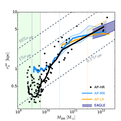
The right-hand panel of Fig. 1 examines convergence in the size of the galaxy (the 3D stellar half-mass radius, , as a function of virial mass. This panel shows that galaxy sizes approach a constant value below a certain, resolution-dependent, virial mass. This may be traced to the combined effects of limited resolution and of the choice of a polytropic equation of state for dense, cold gas in the simulations. As discussed by Crain et al. (2015), the equation of state imposes an effective minimum size for the cold gas in a galaxy which explains the constant size of low-mass galaxies seen in the right-hand panel of Fig. 1.
Notably, the same criterion that ensures convergence for galaxy masses appears to ensure convergence in size, as shown by the shaded regions in the right-hand panel, which extend down to the same minimum mass as in the left-hand panel. The only exception seems to be AP-HR, where the minimum size is reached at . We shall hereafter adopt that mass as the minimum halo mass required for convergence for AP-HR. We summarize in Table 1 the minimum virial mass, , of simulated galaxies retained for further analysis.
3.2 Gas content and sizes
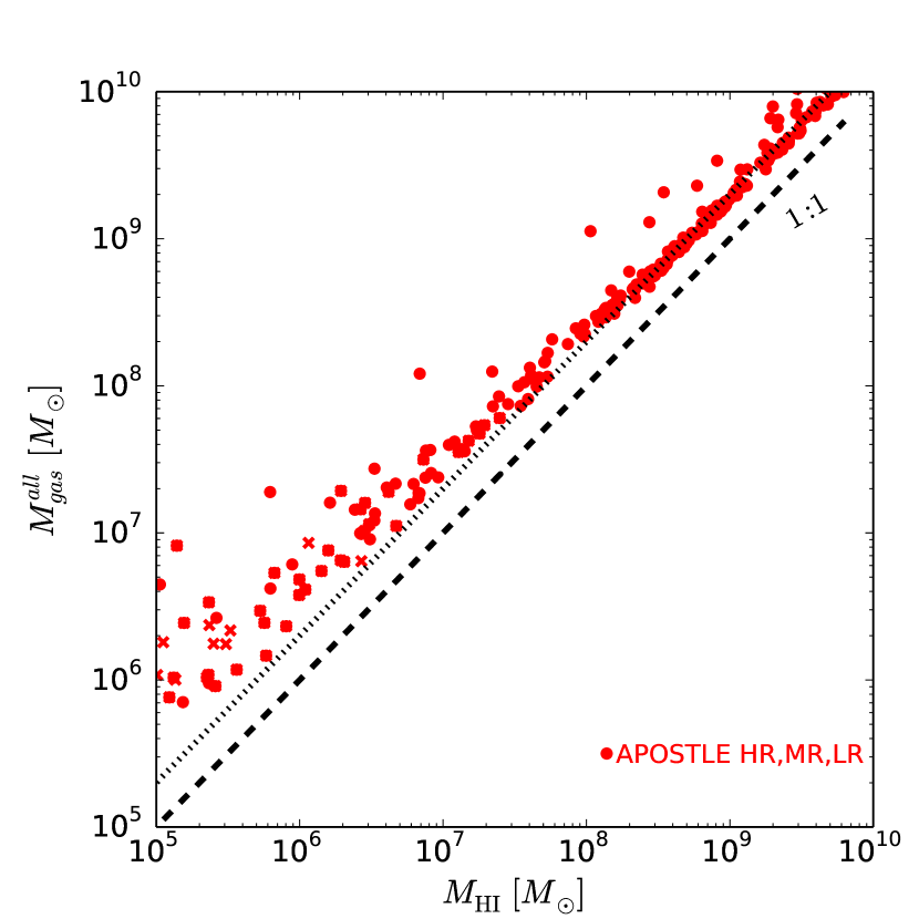
Having established numerical convergence criteria for the baryonic mass and size of simulated galaxies—two of the most important ingredients of the BTF relation—we now assess whether “converged” galaxies compare favourably with observation in terms of their gas, size, and stellar content. Estimates of gas mass in observations are usually derived directly from measurements of neutral hydrogen scaled up by a factor of or in order to take into account the contribution of helium and heavier elements. We note, however, that such a procedure can seriously underpredict the total amount of gas, especially for low-mass galaxies, where ionized gas is expected to be an important contributor. Fig. 2 shows the comparison between the total amount of gas within and that in neutral hydrogen (HI) for our simulated galaxies ( is computed by applying the prescription presented in Appendix A.2 of Rahmati, Pawlik & et al. 2013). At high masses the relation is linear with (dotted line), but below , a simple scaling of the neutral hydrogen mass can severely underestimate the total amount of gas in the galaxy due to increasing importance of ionised gas (see also Gnedin, 2012).
We choose therefore to mimic established practice and, in what follows, we shall estimate gas masses in simulated galaxies by in order to compare with observations. We emphasize, however, that none of our conclusions would change qualitatively if we had used the total amount of gas instead.
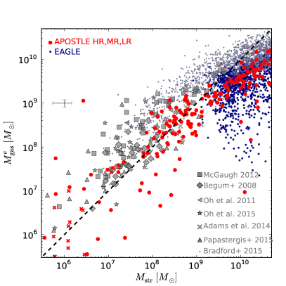
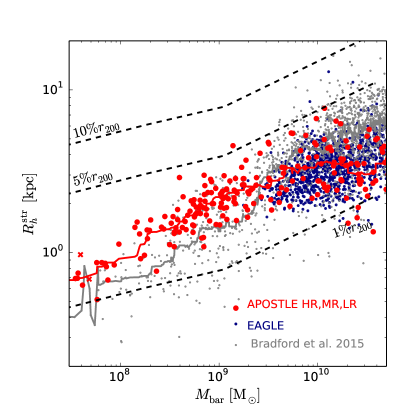
Fig. 3 shows the gas vs stellar mass (left panel), as well as the baryonic mass vs (projected) stellar half-mass radius of simulated galaxies, compared with a compilation of observational surveys, as listed in the legends222Data taken from Begum et al. (2008); Oh et al. (2011); McGaugh (2012); Adams et al. (2014); Oh et al. (2015); Bradford, Geha & Blanton (2015). Additionally, we include a subset of the galaxy compilation in Papastergis et al. (2015), including data from the “Survey of HI in Extremely Low-mass Dwarfs, SHIELDS” (Cannon et al., 2011), the “Local Volume HI Survey, LVHIS” (Trachternach et al., 2009; Kirby et al., 2012), and Leo P (Bernstein-Cooper et al., 2014). Note that for consistency with observations, in the right panel of Fig. 3 sizes in the simulations are computed in 2D, by projecting all star particles along a random line-of-sight direction.
This comparison shows that our galaxies reproduce observed trends relatively well, although some differences are worth pointing out. One is the characteristic galaxy mass below which the gas content dominates the baryonic inventory of a galaxy, which happens for in observed galaxies. In the simulations, although gas is more abundant in low-mass galaxies than in large ones, it rarely dominates the baryonic mass, with an average contribution of about half for galaxies with stellar masses . On average, is a factor - smaller in simulations than in observations at fixed . Interestingly, this factor is independent of baryonic mass, suggesting that the star-formation efficiency in the simulations may be too high by a similar factor at all masses.
The second point to note is that the stellar component of simulated galaxies at the faint end tends to be slightly larger in size, at fixed , than for the observed counterparts ( effect). The reasonable agreement in mass and sizes between observations and simulations implies that estimates of the disk circular velocity from our simulations can reliably be compared with observational measurements.
3.3 The Baryonic Tully-Fisher relation
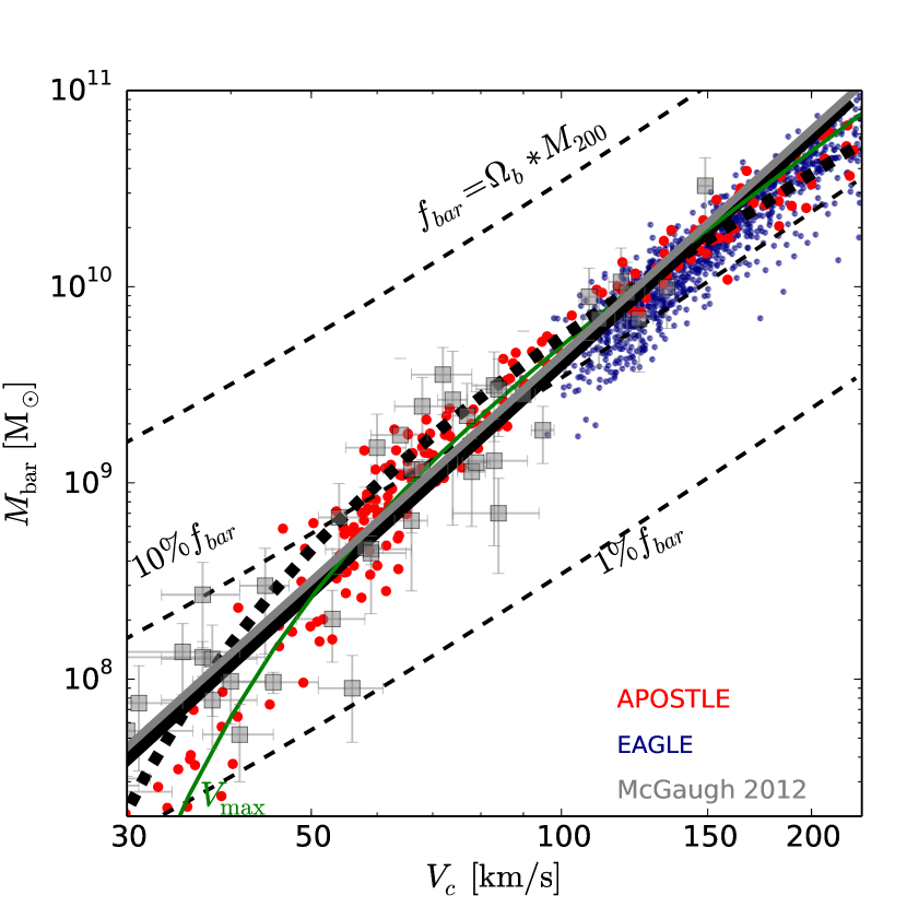
We now proceed to examine the velocity scaling of the baryonic masses. The simulated baryonic Tully-Fisher relation is shown in Fig. 4, where we plot the circular velocity () estimated at twice the baryonic half-mass radius, , vs , the sum of the stellar and gas mass (computed as ) within . We focus in this figure on galaxies with rotation speeds exceeding km/s, which includes most galaxies traditionally used in BTF observational studies, and defer to the next section the analysis of the relation at the very faint end.
A power law fit to the simulated BTF over this velocity range suggests a relation km/s (as shown by the black solid line). This may be compared with data for individual galaxies from the compilation of McGaugh (2012), which are shown by the grey squares with error bars, as well as with the power-law fit provided by that reference, km/s, indicated by the thick grey line.
The differences between the simulated and observed BTF relations are not large, especially considering that we are using all simulated galaxies in the comparison, without selecting for gas content, size, morphology, or rotational support. Galaxies in the observed compilation, on the other hand, are mainly disk systems where the gas component dominates333These were purposefully chosen to be gas-dominated in order to minimize uncertainties on their baryonic masses that arise from poorly-constrained stellar mass-to-light ratios. and where the rotation curve extends sufficiently far to reach the asymptotic maximum of the rotation curve. Although we do not attempt to match such selection procedures in the simulations, the offset between observed and simulated BTF relations is quite small (at most in velocity for galaxies with baryonic mass of order ) and would only improve further if we used the maximum asymptotic velocity for the simulated galaxies. The latter is shown by the thin green solid line labelled “”, which shows the fit to the median relation between and as given in Table 2 (see also Oman et al. 2015).
The agreement between simulated and observed BTF relations shown in Fig. 4 seems to arise naturally in CDM simulations that broadly reproduce the galaxy mass function and the sizes of galaxies as a function of mass. Its normalization at the luminous end is determined primarily by the need to match the number density of galaxies. This fixes the average galaxy formation efficiency in halos of virial mass , assigning them a galaxy like the Milky Way (i.e., ).
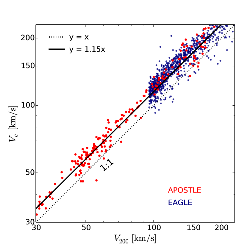
The virial velocity of such halos, km/s, is only slightly below the km/s derived from the observed BTF relation (grey line in Fig. 4), implying that agreement between simulation and observation follows if the circular velocity traced by the baryons is approximately greater than their virial velocity. This is indeed the case for the whole sample, as shown Fig. 5, where we plot the circular velocity at as a function of virial velocity for all simulated galaxies. A simple proportionality links, on average, these two measures; i.e., (see thick dashed line in Fig. 5 showing the median of the points very close to the one-to-one line), exactly what is needed to reconcile the normalization of the simulated and observed BTF relations.
We emphasize that this is not a trivial result, but rather a consequence of the combined effects of (i) the self-similar nature of CDM halos, which regulates the total amount of dark matter enclosed within the luminous region of a galaxy; (ii) the mass and size of the galaxy, which specifies the baryonic contribution to the disk rotation velocity; and (iii) the response of the dark halo to the assembly of the galaxy, which determines how the halo contracts/expands as baryons collect at its center. The agreement between observed and simulated BTF shown in Fig. 4 should therefore be considered a major success of this CDM model of galaxy formation.
The simulations also clarify why the simulated BTF relation is steeper than the “natural” relation discussed in Sec. 1. Since rotation velocities are directly proportional to virial velocity (Fig. 5), the steeper slope mainly reflects the fact that galaxy formation efficiency declines gradually but steadily with decreasing halo mass, as required to match the faint-end of the galaxy stellar mass function (see left-hand panel of Fig. 1).
The response of the dark halo in the EAGLE/APOSTLE simulations has been discussed in detail in Schaller et al. (2015b, c). We shall not repeat that analysis here, except to point out that, for radii as large as , it can be characterized fairly accurately by some mild “adiabatic” contraction, which is only noticeable in the most massive, baryon-dominated galaxies. The galaxy formation efficiency in dwarf galaxy halos is so low that their inner dark mass profiles are unaffected by the assembly of the galaxies (see also the discussion in Oman et al., 2015).
Finally, we consider the scatter in the simulated BTF relation. A conservative estimate may be derived by considering all simulated galaxies, regardless of morphological type, size, gas fraction, or rotation curve shape. We find an rms scatter of dex in mass and dex in velocity from the best power-law fit to the data shown in Fig. 4. The scatter is even smaller if, instead of a power law, one considers a relation whose slope steepens slightly toward the faint end444These fits are of the form , where is the velocity in units of km/s. The best fit parameters , , and are listed in Table 2.. The scatter about this relation is just dex in mass and dex in velocity. For comparison, the power-law scatter in the observed BTF relation shown in Fig. 4 is dex in mass and dex in velocity. We conclude that our simulations have no obvious difficulty accounting for the small scatter in the BTF relation. Actually, the opposite seems true once fainter galaxies are considered, as we discuss next.
| Relation | |||
|---|---|---|---|
| 3.08 | -2.43 | ||
| 2.5 | -2.00 |
3.4 The faint end of the BTF relation
The discussion of the previous section has important consequences for the faint end of the BTF relation. If galaxy formation efficiencies drop ever more rapidly with decreasing halo mass (as shown in the left-hand panel of Fig. 1), a sharp steepening of the BTF relation should be expected at the faint end. This is shown explicitly by the thin green line labeled “” in Fig. 4, which shows the median baryonic mass as a function of the maximum asymptotic circular velocity for simulated galaxies. The faint-end steepening is a direct consequence of the increased efficiency of feedback in shallower potential wells, and is therefore a robust prediction of the model.
In order to examine whether this prediction agrees with observation, we need to extend the observational sample to include fainter galaxies than those listed in the compilation of McGaugh (2012). We therefore add to the observed sample galaxies from the THINGS (de Blok et al., 2008; Oh et al., 2011) and LITTLE THINGS (Oh et al., 2015) surveys; those from the compilation of Papastergis et al. (2015); as well as individual galaxies observed by Begum et al. (2008) and Adams et al. (2014).
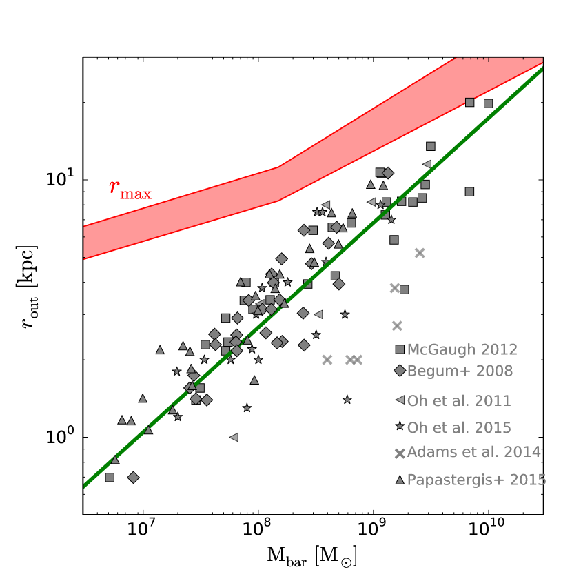
One issue that arises when enlarging the dwarf galaxy sample in this manner is that in many cases the rotation curve is still rising at the outermost measured radius and therefore the reported velocity may fall short of the maximum asymptotic value of the system. One way of appreciating this is shown in Fig. 6, where we plot the outermost radius of the rotation curve, , vs baryonic mass for all the galaxies in the references listed above. Clearly, the observed radial extent of the rotation curve correlates strongly with baryonic mass: the lower the galaxy mass the smaller the galaxy and the shorter its rotation curve. This is in sharp contrast with the radius, , at which the maximum circular velocity is reached in simulated galaxies, which flattens out at small masses as a result of the steepening of the - relation. Broadly speaking, all dwarfs in Fig. 6 with baryonic masses below inhabit halos of similar virial mass, which results in the very weak dependence of with shown in this figure.
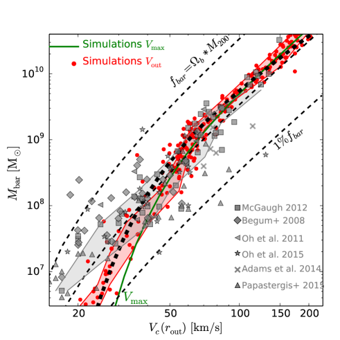
Because is in many cases much smaller than , especially at the low-mass end, it is important that velocities are estimated at similar radii when comparing with observations. We attempt to do this by choosing a value of for each simulated galaxy based on its baryonic mass and by randomly sampling the - relation shown in Fig. 6. (In practice we use the power-law fit shown by the solid green line and a Gaussian scatter in radius of dex.). This procedure ensures that that circular velocities are measured for our simulated galaxies at the same radii on average as for observed galaxies of the same baryonic mass. Note that for the small masses of most interest in this paper, both simulated and observed systems are usually dominated by dark matter, so that that the actual distribution of baryons has little effect.
The result of this exercise is shown in Fig. 7, where red solid circles show the predicted for simulated galaxies and the shaded areas bracket the interquartile velocity distribution obtained (at fixed ). The comparison illustrates a couple of interesting points. One is that, as expected, the rotation velocities at the faint end underestimate the maximum circular velocities by, at times, a fairly large factor. This has the effect of largely rectifying the BTF steepening predicted when using so that the relation at the faint end appears to follow a power-law scaling similar to that of the more luminous systems (see Brook & Di Cintio, 2015, for a similar analysis and conclusion). The sharp steepening of the BTF at the faint end may thus be somewhat “hidden” by the fact that the sizes of galaxies scale strongly with baryonic mass, leading to a systematically larger underestimation of the maximum circular velocity with decreasing galaxy mass (see discussion in Papastergis & Shankar, 2015).
Fig. 7 also highlights a few differences between the observed and simulated the BTF relation at the faint end: (i) the scatter in velocity at given mass is significantly larger in observations, and (ii) the steepening trend seen in the simulated BTF faint end is more pronounced than observed, despite the rectifying effect caused by the small values of discussed above.
The first point may be best appreciated by considering the dispersion in simulated velocities at given mass, which is basically independent of and only of order dex when measured from the best-fit function shown by the thick black dashed line. On the other hand, the dispersion in the observed data is much greater: for example, at the velocity rms is dex, with some obvious outliers in the observed sample for which there are no simulated counterparts.
The second point suggests that, at the very faint end, observed galaxies inhabit halos of lower mass (or lower circular velocity, to be more precise) than predicted by the model, a result reminiscent of previous conclusions (Ferrero et al., 2012; Papastergis et al., 2015). A similar issue arises when comparing the predicted and estimated masses of Milky Way satellites, also known as the “too-big-to-fail” problem (Boylan-Kolchin, Bullock & Kaplinghat, 2011). The difference is, however, small: the median velocity predicted for galaxies in the range is km/s while the observed value is km/s.
The observed outliers in Fig. 7 present a more worrying puzzle. The ones to the right of the simulated trend can in principle be explained as baryon-dominated galaxies where the central concentration of baryonic matter leads to rotation velocities that exceed the asymptotic maximum of the halo (i.e., “declining” rotation curves). The ones on the left, on the other hand, are more difficult to explain. These are galaxies that are extremely massive in baryons for their rotation speed or, alternatively, that rotate much more slowly than is typical for their mass.
Because galaxy formation efficiencies are, almost without exception, very low in simulated dwarf galaxies, the observed baryonic mass of a galaxy places a strong lower limit on the virial mass of the halo it inhabits. The mass of the halo then constrains the total amount of dark matter within , placing a strong lower limit on the circular velocity there. The outliers on the left of the simulated trend shown in Fig. 7 are therefore either systems with uncharacteristically high galaxy formation efficiency, or else systems with unusually low dark matter content within for their virial mass.
If these galaxies are rotationally supported (such that their measured rotation speed is equal to their circular velocity ), the latter option implies that some dark matter is “missing” from the inner regions of the halo, leading to a circular velocity at that substantially underestimate the true maximum circular velocity of the system. It would be tempting to ascribe this result to the presence of “cores” in the dark halo but we note that this would imply cores larger than the galaxy itself. Furthermore, in that case all such outliers should have rising rotation curves that extend out to at least . That is indeed the case for the one simulated point close to the efficiency line (top dashed curve in Fig. 7). In that case a rotation velocity of km/s is measured at kpc, whereas the asymptotic maximum velocity of km/s is not reached until kpc. On the other hand, as discussed by (Oman et al., 2016), the rotation curves of the observed outliers are typically not rising at their outermost radius.
Inclination errors could also potentially bring some of the outliers back to the main relation. This would, however, require inclination corrections of order , well above the estimated uncertainties in current observations (see detailed discussion in Oman et al. 2016). If more accurate measurements of inclination angles confirm the current estimates, these outliers are truly systems without explanation in our CDM-based model of galaxy formation.
4 Summary and Conclusions
We use the APOSTLE/EAGLE suite of cosmological hydrodynamical simulations to examine the scaling between baryonic mass and rotation velocity (the “Baryonic Tully-Fisher” relation, BTF) of galaxies formed in a CDM universe. Our main conclusions may be summarized as follows.
We find that the observed BTF relation is reproduced, without further tuning, by galaxy formation simulations that reproduce the galaxy stellar mass function and predict galaxy sizes comparable to observed values. This implies that: (i) the BTF normalization is largely determined by matching the abundance of galaxies; (ii) the slope results from the steady decline in galaxy formation efficiency with decreasing virial mass. Through a fortuitous combination of competing effects, the galaxy rotation velocities end up being, on average, almost equal to the halo virial velocities (). The scatter in the simulated BTF relation is slightly smaller than observed, despite the strong feedback-driven winds that regulate gas accretion and star formation in the simulations.
The agreement between observed and simulated BTF relations does not require, in our simulations, any special adjustment of the inner dark matter density profile (such as the creation of a constant-density “core” or a substantial expansion of the central cusp) except for a mild contraction of the halo in baryon-dominated systems.
At the very faint end (i.e., rotation velocities km/s) the simulated BTF relation steepens considerably in mass as a result of the sharp drop in galaxy formation efficiencies in low-mass halos that is required to match the shallow faint-end of the galaxy stellar mass function. This implies that most faint dwarfs (i.e., ) should inhabit halos of very similar virial mass and, consequently, similar maximum circular velocities.
The observed steepening of the BTF relation at the faint end is less pronounced, and is accompanied by larger scatter than expected from the simulations. This disagreement may be reduced by accounting for the fact that low-mass galaxies are small: their rotation curves probe only the rising part of the halo circular velocity profile, leading to systematic underestimation of the asymptotic maximum circular velocity.
More difficult to reconcile with simulations is the large scatter at the faint end of the observed BTF relation. The presence of fairly massive galaxies with unexpectedly small rotation velocities is particularly difficult to explain. This is because, given the small galaxy formation efficiency of low-mass halos inherent to our model, the baryonic mass of a galaxy places a strong lower limit on the halo mass it inhabits, implying much higher velocities than observed. Unless the interpretation of the observational data is in substantial error (perhaps due to severe underestimation of galaxy inclinations) these outliers seem to be either “missing dark matter” from the inner regions of their halos, or to have experienced extraordinarily efficient galaxy formation (Oman et al., 2016). Neither possibility is accounted for in our model, and therefore such systems have no counterparts in our simulations.
Acknowledgments
The authors wish to thank S.-H. Oh, E. de Blok, J. Adams, M. Papastergis and J. Bradford for making data available in electronic form. JFN acknowledges a Leverhulme Trust Visiting Professorship hosted at the ICC by CSF. This work was supported by the Science and Technology Facilities Council (grant number ST/F001166/1). RAC is a Royal Society University Research Fellow. CSF acknowledges ERC Advanced Grant 267291 ”COSMIWAY” and JFN a Leverhulme Visiting Professor grant held at the Institute for Computational Cosmology, Durham University. This work used the DiRAC Data Centric system at Durham University, operated by the Institute for Computational Cosmology on behalf of the STFC DiRAC HPC Facility (www.dirac.ac.uk). This equipment was funded by BIS National E-infrastructure capital grant ST/K00042X/1, STFC capital grant ST/H008519/1, and STFC DiRAC Operations grant ST/K003267/1 and Durham University. DiRAC is part of the National E-Infrastructure. The research was supported in part by the European Research Council under the European Union Seventh Framework Programme (FP7/2007-2013) / ERC Grant agreement 278594-GasAroundGalaxies.
References
- Abadi et al. (2003) Abadi M. G., Navarro J. F., Steinmetz M., Eke V. R., 2003, ApJ, 591, 499
- Adams et al. (2014) Adams J. J., Simon J. D., Fabricius M. H., et al., 2014, ApJ, 789, 63
- Aumer et al. (2013) Aumer M., White S. D. M., Naab T., Scannapieco C., 2013, MNRAS, 434, 3142
- Begum et al. (2008) Begum A., Chengalur J. N., Karachentsev I. D., Sharina M. E., 2008, MNRAS, 386, 138
- Bell & de Jong (2001) Bell E. F., de Jong R. S., 2001, ApJ, 550, 212
- Bernstein-Cooper et al. (2014) Bernstein-Cooper E. Z., Cannon J. M., Elson E. C., Warren S. R., Chengular J., et al., 2014, AJ, 148, 35
- Booth & Schaye (2009) Booth C. M., Schaye J., 2009, MNRAS, 398, 53
- Boylan-Kolchin, Bullock & Kaplinghat (2011) Boylan-Kolchin M., Bullock J. S., Kaplinghat M., 2011, MNRAS, 415, L40
- Bradford, Geha & Blanton (2015) Bradford J. D., Geha M. C., Blanton M. R., 2015, ArXiv e-prints 1505.04819
- Brook & Di Cintio (2015) Brook C. B., Di Cintio A., 2015, MNRAS, 453, 2133
- Brook et al. (2012) Brook C. B., Stinson G., Gibson B. K., Wadsley J., Quinn T., 2012, MNRAS, 424, 1275
- Cannon et al. (2011) Cannon J. M., Giovanelli R., Haynes M. P., Janowiecki S., Parker A., Salzer J. J., et al., 2011, ApJL, 739, L22
- Chan et al. (2015) Chan T. K., Kereš D., Oñorbe J., Hopkins P. F., Muratov A. L., Faucher-Giguère C.-A., Quataert E., 2015, MNRAS, 454, 2981
- Cole et al. (2000) Cole S., Lacey C. G., Baugh C. M., Frenk C. S., 2000, MNRAS, 319, 168
- Crain et al. (2015) Crain R. A., Schaye J., Bower R. G., Furlong M., Schaller M., Theuns T., et al., 2015, MNRAS, 450, 1937
- Dalla Vecchia & Schaye (2008) Dalla Vecchia C., Schaye J., 2008, MNRAS, 387, 1431
- Dalla Vecchia & Schaye (2012) Dalla Vecchia C., Schaye J., 2012, MNRAS, 426, 140
- Davis et al. (1985) Davis M., Efstathiou G., Frenk C. S., White S. D. M., 1985, ApJ, 292, 371
- de Blok et al. (2008) de Blok W. J. G., Walter F., Brinks E., Trachternach C., Oh S.-H., Kennicutt, Jr. R. C., 2008, AJ, 136, 2648
- Dolag et al. (2009) Dolag K., Borgani S., Murante G., Springel V., 2009, MNRAS, 399, 497
- Dutton & van den Bosch (2009) Dutton A. A., van den Bosch F. C., 2009, MNRAS, 396, 141
- Fattahi et al. (2016) Fattahi A. et al., 2016, MNRAS, 457, 844
- Ferrero et al. (2012) Ferrero I., Abadi M. G., Navarro J. F., Sales L. V., Gurovich S., 2012, MNRAS, 425, 2817
- Geha et al. (2006) Geha M., Blanton M. R., Masjedi M., West A. A., 2006, ApJ, 653, 240
- Gnedin (2012) Gnedin N. Y., 2012, ApJ, 754, 113
- Governato et al. (2004) Governato F. et al., 2004, ApJ, 607, 688
- Guedes et al. (2011) Guedes J., Callegari S., Madau P., Mayer L., 2011, ApJ, 742, 76
- Hopkins (2013) Hopkins P. F., 2013, MNRAS, 428, 2840
- Kirby et al. (2012) Kirby E. M., Koribalski B., Jerjen H., López-Sánchez Á., 2012, MNRAS, 420, 2924
- Komatsu et al. (2011) Komatsu E., Smith K. M., Dunkley J., Bennett C. L., Gold B., et al., 2011, ApJS, 192, 18
- Lacey et al. (2015) Lacey C. G. et al., 2015, ArXiv e-prints 1509.08473
- Lelli, McGaugh & Schombert (2016) Lelli F., McGaugh S. S., Schombert J. M., 2016, ApJL, 816, L14
- Marinacci, Pakmor & Springel (2014) Marinacci F., Pakmor R., Springel V., 2014, MNRAS, 437, 1750
- McCarthy et al. (2012) McCarthy I. G., Schaye J., Font A. S., Theuns T., Frenk C. S., Crain R. A., Dalla Vecchia C., 2012, MNRAS, 427, 379
- McGaugh (2012) McGaugh S. S., 2012, AJ, 143, 40
- McGaugh et al. (2000) McGaugh S. S., Schombert J. M., Bothun G. D., de Blok W. J. G., 2000, ApJL, 533, L99
- Mo, Mao & White (1998) Mo H. J., Mao S., White S. D. M., 1998, MNRAS, 295, 319
- Navarro & Steinmetz (2000) Navarro J. F., Steinmetz M., 2000, ApJ, 528, 607
- Oh et al. (2011) Oh S.-H., de Blok W. J. G., Brinks E., Walter F., Kennicutt, Jr. R. C., 2011, AJ, 141, 193
- Oh et al. (2015) Oh S.-H., Hunter D. A., Brinks E., et al., 2015, AJ, 149, 180
- Oman et al. (2015) Oman K. A. et al., 2015, MNRAS, 452, 3650
- Oman et al. (2016) Oman K. A., Navarro J. F., Sales L. V., Fattahi A., Frenk C. S., Sawala T., Schaller M., White S. D. M., 2016, ArXiv e-prints 1601.01026
- Papastergis et al. (2015) Papastergis E., Giovanelli R., Haynes M. P., Shankar F., 2015, A&A, 574, A113
- Papastergis & Shankar (2015) Papastergis E., Shankar F., 2015, ArXiv e-prints 1511.08741
- Pizagno et al. (2005) Pizagno J. et al., 2005, ApJ, 633, 844
- Planck Collaboration et al. (2014) Planck Collaboration, Ade P. A. R., Aghanim N., Alves M. I. R., Armitage-Caplan C., et al., 2014, A&A, 571, A1
- Rahmati, Pawlik & et al. (2013) Rahmati A., Pawlik A. H., et al., 2013, MNRAS, 430, 2427
- Rix & Bovy (2013) Rix H.-W., Bovy J., 2013, A&ARv, 21, 61
- Rosas-Guevara et al. (2015) Rosas-Guevara Y. M. et al., 2015, MNRAS, 454, 1038
- Sawala et al. (2015) Sawala T., Frenk C. S., Fattahi A., Navarro J. F., Bower R. G., Crain R. A., et al., 2015, ArXiv e-prints 1511.01098
- Scannapieco et al. (2012) Scannapieco C., Wadepuhl M., Parry O. H., Navarro J. F., et al., 2012, MNRAS, 423, 1726
- Schaller et al. (2015a) Schaller M., Dalla Vecchia C., Schaye J., Bower R. G., Theuns T., Crain R. A., Furlong M., McCarthy I. G., 2015a, MNRAS, 454, 2277
- Schaller et al. (2015b) Schaller M., Frenk C. S., Bower R. G., Theuns T., Jenkins A., Schaye J., et al., 2015b, MNRAS, 451, 1247
- Schaller et al. (2015c) Schaller M., Frenk C. S., Bower R. G., Theuns T., Trayford J., et al., 2015c, MNRAS, 452, 343
- Schaye (2004) Schaye J., 2004, ApJ, 609, 667
- Schaye et al. (2015) Schaye J., Crain R. A., Bower R. G., et al., 2015, MNRAS, 446, 521
- Springel (2005) Springel V., 2005, MNRAS, 364, 1105
- Springel, Di Matteo & Hernquist (2005) Springel V., Di Matteo T., Hernquist L., 2005, MNRAS, 361, 776
- Springel et al. (2001) Springel V., White S. D. M., Tormen G., Kauffmann G., 2001, MNRAS, 328, 726
- Stark, McGaugh & Swaters (2009) Stark D. V., McGaugh S. S., Swaters R. A., 2009, AJ, 138, 392
- Steinmetz & Navarro (1999) Steinmetz M., Navarro J. F., 1999, ApJ, 513, 555
- Torres-Flores et al. (2011) Torres-Flores S., Epinat B., Amram P., Plana H., Mendes de Oliveira C., 2011, MNRAS, 416, 1936
- Trachternach et al. (2009) Trachternach C., de Blok W. J. G., McGaugh S. S., van der Hulst J. M., Dettmar R.-J., 2009, A&A, 505, 577
- Trayford et al. (2015) Trayford J. W. et al., 2015, MNRAS, 452, 2879
- Tully & Fisher (1977) Tully R. B., Fisher J. R., 1977, A&A, 54, 661
- Verheijen (2001) Verheijen M. A. W., 2001, ApJ, 563, 694
- Vogelsberger et al. (2014) Vogelsberger M., Zavala J., Simpson C., Jenkins A., 2014, MNRAS, 444, 3684
- White & Frenk (1991) White S. D. M., Frenk C. S., 1991, ApJ, 379, 52
- Wiersma, Schaye & Smith (2009) Wiersma R. P. C., Schaye J., Smith B. D., 2009, MNRAS, 393, 99
- Wiersma et al. (2009) Wiersma R. P. C., Schaye J., Theuns T., Dalla Vecchia C., Tornatore L., 2009, MNRAS, 399, 574