A Sparse Grid Discontinuous Galerkin Method for High-Dimensional Transport Equations and Its Application to Kinetic Simulations

Wei Guo Department of Mathematics, Michigan State University, East Lansing, MI 48824 U.S.A. wguo@math.msu.edu    Yingda Cheng Department of Mathematics, Michigan State University, East Lansing, MI 48824 U.S.A. ycheng@math.msu.edu. Research is supported by NSF grants DMS-1318186 and DMS-1453661.
Abstract

In this paper, we develop a sparse grid discontinuous Galerkin (DG) scheme for transport equations and applied it to kinetic simulations. The method uses the weak formulations of traditional Runge-Kutta DG (RKDG) schemes for hyperbolic problems and is proven to be L2superscript𝐿2L^{2} stable and convergent. A major advantage of the scheme lies in its low computational and storage cost due to the employed sparse finite element approximation space. This attractive feature is explored in simulating Vlasov and Boltzmann transport equations. Good performance in accuracy and conservation is verified by numerical tests in up to four dimensions.

keywords:
discontinuous Galerkin methods; sparse grid; high-dimensional transport equations; Vlasov equation; Boltzmann equation.

1 Introduction

In this paper, we develop a sparse grid DG method for high-dimensional transport equations. High-dimensional transport problems are ubiquitous in science and engineering, and most evidently in kinetic simulations where it is necessary to track the evolution of probability density functions of particles. Deterministic kinetic simulations are very demanding due to the large computational and storage cost. To make the schemes more attractive comparing with the alternative probabilistic methods, an appealing approach is to explore the sparse grid techniques [6, 15] with the aim of breaking the curse of dimensionality [4]. In the context of wavelets or sparse grid methods for kinetic transport equations, we mention the work of using wavelet-MRA methods for Vlasov equations [5], the combination technique for linear gyrokinetics [19], sparse adaptive finite element method [25], sparse discrete ordinates method [16] and sparse tensor spherical harmonics [17] for radiative transfer, among many others.

This paper focuses on the DG method [13], which is a class of finite element methods using discontinuous approximation space for the numerical solution and the test functions. The RKDG scheme [14] developed in a series of papers for hyperbolic equations became very popular due to its provable convergence, excellent conservation properties and accommodation for adaptivity and parallel implementations. Recent years have seen great growth in the interest of applying DG methods to kinetic systems (see for example [3, 18, 20, 9, 10]) because of the conservation properties and long time performance of the resulting simulations. However, the DG method is still deemed too costly in a realistic setting, often requiring more degrees of freedom than other high order numerical calculations.

Recently, we developed a sparse grid DG method for high-dimensional elliptic problems [24]. A sparse DG finite element space has been constructed, reducing the degrees of freedom from the standard O(hd)𝑂superscript𝑑O(h^{-d}) to O(h1|log2h|d1)𝑂superscript1superscriptsubscript2𝑑1O(h^{-1}|\log_{2}h|^{d-1}) for d𝑑d-dimensional problems, where hh is the uniform mesh size in each dimension. The resulting scheme retains main properties of standard DG methods while making the computational cost tangebile for high-dimensional simulations. This motivates the current work for the transport equations, and we use kinetic problems as a test bed for the new algorithm. The scheme in this paper uses weak formulation to guarantee many nice properties such as stability and conservation, while a detailed study of the approximation results is performed to obtain L2superscript𝐿2L^{2} convergence rate of O((logh)dhk+1/2)𝑂superscript𝑑superscript𝑘12O((\log h)^{d}h^{k+1/2}) for smooth enough solutions, where k𝑘k is the degree of polynomial. The method is demonstrated to be advantageous for kinetic simulations, because it can capture the main features of the solution with manageable cost and can conserve key macroscopic quantities in the mean time. The rest of this paper is organized as follows: in Section 2, we construct the sparse grid DG formulations for linear transport equation with variable coefficient. In Section 3, we prove L2superscript𝐿2L^{2} stability and error estimate for constant coefficient equations. The numerical performance is validated in Section 4 by several benchmark tests. Section 5 discusses the application of the scheme to Vlasov and Boltzmann equations, and we conclude the paper with some remarks and future work in Section 6. The detail of the proof of a key lemma is gathered in the Appendix.

2 Numerical method

In this section, we construct the sparse grid DG method for the following d𝑑d-dimensional linear transport equation with variable coefficients on a box-shaped domain

{ut+(𝒂(t,𝐱)u)=0,𝐱Ω=[0,1]d,u(0,𝐱)=u0(𝐱),casesformulae-sequencesubscript𝑢𝑡𝒂𝑡𝐱𝑢0𝐱Ωsuperscript01𝑑𝑢0𝐱subscript𝑢0𝐱\left\{\begin{array}[]{l}u_{t}+\nabla\cdot({\bm{a}}(t,\mathbf{x})\,u)=0,\quad\mathbf{x}\in\Omega=[0,1]^{d},\\[5.69054pt] u(0,\mathbf{x})=u_{0}(\mathbf{x}),\end{array}\right. (1)

subject to suitable boundary conditions. We first review the DG finite element space on sparse grid introduced in [24], and then provide the formulation of scheme along with implementation details.

2.1 DG finite element space on sparse grid

In this subsection, we prescribe the grid and the associated finite element space. Many of the discussions follow from our previous work for elliptic equations [24]. First, we introduce the hierarchical decomposition of piecewise polynomial space in one dimension on the interval [0,1]01[0,1]. We define a set of nested grids, where the n𝑛n-th level grid ΩnsubscriptΩ𝑛\Omega_{n} consists of 2nsuperscript2𝑛2^{n} uniform cells Inj=(2nj,2n(j+1)]superscriptsubscript𝐼𝑛𝑗superscript2𝑛𝑗superscript2𝑛𝑗1I_{n}^{j}=(2^{-n}j,2^{-n}(j+1)], j=0,,2n1,𝑗0superscript2𝑛1j=0,\ldots,2^{n}-1, for any n0.𝑛0n\geq 0. The nested grids result in the nested piecewise polynomial spaces. In particular, let

Vnk:={v:vPk(Inj),j=0,,2n1}assignsuperscriptsubscript𝑉𝑛𝑘conditional-set𝑣formulae-sequence𝑣superscript𝑃𝑘superscriptsubscript𝐼𝑛𝑗for-all𝑗0superscript2𝑛1V_{n}^{k}:=\{v:v\in P^{k}(I_{n}^{j}),\,\forall\,j=0,\ldots,2^{n}-1\}

be the usual piecewise polynomials of degree at most k𝑘k on the n𝑛n-th level grid ΩnsubscriptΩ𝑛\Omega_{n}. Then, we have

V0kV1kV2kV3ksuperscriptsubscript𝑉0𝑘superscriptsubscript𝑉1𝑘superscriptsubscript𝑉2𝑘superscriptsubscript𝑉3𝑘V_{0}^{k}\subset V_{1}^{k}\subset V_{2}^{k}\subset V_{3}^{k}\subset\cdots

We can now define the multiwavelet subspace Wnksuperscriptsubscript𝑊𝑛𝑘W_{n}^{k}, n=1,2,𝑛12n=1,2,\ldots as the orthogonal complement of Vn1ksuperscriptsubscript𝑉𝑛1𝑘V_{n-1}^{k} in Vnksuperscriptsubscript𝑉𝑛𝑘V_{n}^{k} with respect to the L2superscript𝐿2L^{2} inner product on [0,1]01[0,1], i.e.,

Vn1kWnk=Vnk,WnkVn1k.formulae-sequencedirect-sumsuperscriptsubscript𝑉𝑛1𝑘superscriptsubscript𝑊𝑛𝑘superscriptsubscript𝑉𝑛𝑘perpendicular-tosuperscriptsubscript𝑊𝑛𝑘superscriptsubscript𝑉𝑛1𝑘V_{n-1}^{k}\oplus W_{n}^{k}=V_{n}^{k},\quad W_{n}^{k}\perp V_{n-1}^{k}.

For notational convenience, we let W0k:=V0kassignsuperscriptsubscript𝑊0𝑘superscriptsubscript𝑉0𝑘W_{0}^{k}:=V_{0}^{k}, which is standard piecewise polynomial space of degree k𝑘k on [0,1]01[0,1]. The dimension of Wnksuperscriptsubscript𝑊𝑛𝑘W_{n}^{k} is 2n1(k+1)superscript2𝑛1𝑘12^{n-1}(k+1) when n1𝑛1n\geq 1, and k+1𝑘1k+1 when n=0𝑛0n=0. In summary, we have found a hierarchical representation of the standard piecewise polynomial space Vnksuperscriptsubscript𝑉𝑛𝑘V_{n}^{k} on ΩnsubscriptΩ𝑛\Omega_{n} as Vnk=0jnWjksuperscriptsubscript𝑉𝑛𝑘subscriptdirect-sum0𝑗𝑛superscriptsubscript𝑊𝑗𝑘V_{n}^{k}=\bigoplus_{0\leq j\leq n}W_{j}^{k}.

Now we are ready to review the construction in multi-dimensions. First we recall some basic notations about multi-indices. For a multi-index α=(α1,,αd)0d𝛼subscript𝛼1subscript𝛼𝑑superscriptsubscript0𝑑\mathbf{\alpha}=(\alpha_{1},\cdots,\alpha_{d})\in\mathbb{N}_{0}^{d}, where 0subscript0\mathbb{N}_{0} denotes the set of nonnegative integers, the l1superscript𝑙1l^{1} and lsuperscript𝑙l^{\infty} norms are defined as

|𝜶|1:=m=1dαm,|𝜶|:=max1mdαm.formulae-sequenceassignsubscript𝜶1superscriptsubscript𝑚1𝑑subscript𝛼𝑚assignsubscript𝜶subscript1𝑚𝑑subscript𝛼𝑚|{\bm{\alpha}}|_{1}:=\sum_{m=1}^{d}\alpha_{m},\qquad|{\bm{\alpha}}|_{\infty}:=\max_{1\leq m\leq d}\alpha_{m}.

The component-wise arithmetic operations and relational operations are defined as

𝜶𝜷:=(α1β1,,αdβd),c𝜶:=(cα1,,cαd),2𝜶:=(2α1,,2αd),formulae-sequenceassign𝜶𝜷subscript𝛼1subscript𝛽1subscript𝛼𝑑subscript𝛽𝑑formulae-sequenceassign𝑐𝜶𝑐subscript𝛼1𝑐subscript𝛼𝑑assignsuperscript2𝜶superscript2subscript𝛼1superscript2subscript𝛼𝑑{\bm{\alpha}}\cdot{\bm{\beta}}:=(\alpha_{1}\beta_{1},\ldots,\alpha_{d}\beta_{d}),\qquad c\cdot{\bm{\alpha}}:=(c\alpha_{1},\ldots,c\alpha_{d}),\qquad 2^{\bm{\alpha}}:=(2^{\alpha_{1}},\ldots,2^{\alpha_{d}}),
𝜶𝜷αmβm,m,𝜶<𝜷𝜶𝜷 and 𝜶𝜷.𝜶𝜷formulae-sequencesubscript𝛼𝑚subscript𝛽𝑚for-all𝑚𝜶𝜷𝜶𝜷 and 𝜶𝜷{\bm{\alpha}}\leq{\bm{\beta}}\Leftrightarrow\alpha_{m}\leq\beta_{m},\,\forall m,\quad{\bm{\alpha}}<{\bm{\beta}}\Leftrightarrow{\bm{\alpha}}\leq{\bm{\beta}}\textrm{ and }{\bm{\alpha}}\neq{\bm{\beta}}.

By making use of the multi-index notation, we denote by 𝐥=(l1,,ld)0d𝐥subscript𝑙1subscript𝑙𝑑superscriptsubscript0𝑑\mathbf{l}=(l_{1},\cdots,l_{d})\in\mathbb{N}_{0}^{d} the mesh level in a multivariate sense. We define the tensor-product mesh grid Ω𝐥=Ωl1ΩldsubscriptΩ𝐥tensor-productsubscriptΩsubscript𝑙1subscriptΩsubscript𝑙𝑑\Omega_{\mathbf{l}}=\Omega_{l_{1}}\otimes\cdots\otimes\Omega_{l_{d}} and the corresponding mesh size h𝐥=(hl1,,hld).subscript𝐥subscriptsubscript𝑙1subscriptsubscript𝑙𝑑h_{\mathbf{l}}=(h_{l_{1}},\cdots,h_{l_{d}}). Based on the grid Ω𝐥subscriptΩ𝐥\Omega_{\mathbf{l}}, we denote by I𝐥𝐣={𝐱:xm(hmjm,hm(jm+1)),m=1,,d}superscriptsubscript𝐼𝐥𝐣conditional-set𝐱formulae-sequencesubscript𝑥𝑚subscript𝑚subscript𝑗𝑚subscript𝑚subscript𝑗𝑚1𝑚1𝑑I_{\mathbf{l}}^{\mathbf{j}}=\{\mathbf{x}:x_{m}\in(h_{m}j_{m},h_{m}(j_{m}+1)),m=1,\cdots,d\} an elementary cell, and

𝐕𝐥k:={𝐯:𝐯(𝐱)Pk(I𝐥𝐣),  0𝐣2𝐥𝟏}=Vl1,x1k××Vl1,xdkassignsuperscriptsubscript𝐕𝐥𝑘conditional-set𝐯formulae-sequence𝐯𝐱superscript𝑃𝑘subscriptsuperscript𝐼𝐣𝐥  0𝐣superscript2𝐥1superscriptsubscript𝑉subscript𝑙1subscript𝑥1𝑘superscriptsubscript𝑉subscript𝑙1subscript𝑥𝑑𝑘{\bf V}_{\mathbf{l}}^{k}:=\{{\bf v}:{\bf v}(\mathbf{x})\in P^{k}(I^{\mathbf{j}}_{\mathbf{l}}),\,\,\mathbf{0}\leq\mathbf{j}\leq 2^{\mathbf{l}}-\mathbf{1}\}=V_{l_{1},x_{1}}^{k}\times\cdots\times V_{l_{1},x_{d}}^{k}

the tensor-product piecewise polynomial space, where Pk(I𝐥𝐣)superscript𝑃𝑘subscriptsuperscript𝐼𝐣𝐥P^{k}(I^{\mathbf{j}}_{\mathbf{l}}) denotes the collection of polynomials of degree up to k𝑘k in each dimension on cell I𝐥𝐣subscriptsuperscript𝐼𝐣𝐥I^{\mathbf{j}}_{\mathbf{l}}. If we use equal mesh refinement of size hN=2Nsubscript𝑁superscript2𝑁h_{N}=2^{-N} in each coordinate direction, the grid and space will be denoted by ΩNsubscriptΩ𝑁\Omega_{N} and 𝐕Nksuperscriptsubscript𝐕𝑁𝑘{\bf V}_{N}^{k}, respectively.

Based on a tensor-product construction, the multi-dimensional increment space can be defined as

𝐖𝐥k=Wl1,x1k××Wl1,xdk.superscriptsubscript𝐖𝐥𝑘superscriptsubscript𝑊subscript𝑙1subscript𝑥1𝑘superscriptsubscript𝑊subscript𝑙1subscript𝑥𝑑𝑘\mathbf{W}_{\mathbf{l}}^{k}=W_{l_{1},x_{1}}^{k}\times\cdots\times W_{l_{1},x_{d}}^{k}.

Therefore, space 𝐕𝐥ksuperscriptsubscript𝐕𝐥𝑘{\bf V}_{\mathbf{l}}^{k} can be represented by

𝐕𝐥k=0j1l1,,0jdld𝐖𝐣k.superscriptsubscript𝐕𝐥𝑘subscriptdirect-sumformulae-sequence0subscript𝑗1subscript𝑙10subscript𝑗𝑑subscript𝑙𝑑superscriptsubscript𝐖𝐣𝑘{\bf V}_{\mathbf{l}}^{k}=\bigoplus_{0\leq j_{1}\leq l_{1},\ldots,0\leq j_{d}\leq l_{d}}\mathbf{W}_{\mathbf{j}}^{k}.

In particular, we have the standard tensor-product polynomial space on ΩNsubscriptΩ𝑁\Omega_{N} as

𝐕Nk=|𝐥|N𝐥0d𝐖𝐥k.superscriptsubscript𝐕𝑁𝑘subscriptdirect-sumsubscript𝐥𝑁𝐥superscriptsubscript0𝑑superscriptsubscript𝐖𝐥𝑘{\bf V}_{N}^{k}=\bigoplus_{\begin{subarray}{c}|\mathbf{l}|_{\infty}\leq N\\ \mathbf{l}\in\mathbb{N}_{0}^{d}\end{subarray}}\mathbf{W}_{\mathbf{l}}^{k}.

The sparse finite element approximation space on ΩNsubscriptΩ𝑁\Omega_{N} we use in this paper, on the other hand, is defined by

𝐕^Nk:=|𝐥|1N𝐥0d𝐖𝐥k.assignsuperscriptsubscript^𝐕𝑁𝑘subscriptdirect-sumsubscript𝐥1𝑁𝐥superscriptsubscript0𝑑superscriptsubscript𝐖𝐥𝑘\hat{{\bf V}}_{N}^{k}:=\bigoplus_{\begin{subarray}{c}|\mathbf{l}|_{1}\leq N\\ \mathbf{l}\in\mathbb{N}_{0}^{d}\end{subarray}}\mathbf{W}_{\mathbf{l}}^{k}.

This is a subset of 𝐕Nksuperscriptsubscript𝐕𝑁𝑘{\bf V}_{N}^{k}, and its number of degrees of freedom scales as O((k+1)d2NNd1)𝑂superscript𝑘1𝑑superscript2𝑁superscript𝑁𝑑1O((k+1)^{d}2^{N}N^{d-1}) [24], which is significantly less than that of 𝐕Nksuperscriptsubscript𝐕𝑁𝑘{\bf V}_{N}^{k} with exponential dependence on Nd𝑁𝑑Nd. This is the key for computational savings in high dimensions.

2.2 Formulation of the scheme

In this subsection, we formulate a DG scheme with the sparse finite element space 𝐕^Nksuperscriptsubscript^𝐕𝑁𝑘\hat{{\bf V}}_{N}^{k} for solving the model problem (1). For simplicity of discussion, we assume periodic boundary conditions but note that the discussion can be easily generalized to Dirichlet boundary conditions as well. First, we review some basic notations about jumps and averages for piecewise functions defined on the grid ΩNsubscriptΩ𝑁\Omega_{N}. Let Thsubscript𝑇T_{h} be the collection of all elementary cell IN𝐣,0jm2N1,m=1,,dformulae-sequencesubscriptsuperscript𝐼𝐣𝑁0subscript𝑗𝑚superscript2𝑁1for-all𝑚1𝑑I^{\mathbf{j}}_{N},\quad 0\leq j_{m}\leq 2^{N}-1,\forall\,m=1,\ldots,d. Γ:=TΩNTassignΓsubscript𝑇subscriptΩ𝑁subscript𝑇\Gamma:=\bigcup_{T\in\Omega_{N}}\partial_{T} be the union of the interfaces for all the elements in ΩNsubscriptΩ𝑁\Omega_{N} (here we have taken into account the periodic boundary condition when defining ΓΓ\Gamma) and S(Γ):=ΠTΩNL2(T)assign𝑆ΓsubscriptΠ𝑇subscriptΩ𝑁superscript𝐿2𝑇S(\Gamma):=\Pi_{T\in\Omega_{N}}L^{2}(\partial T) be the set of L2superscript𝐿2L^{2} functions defined on ΓΓ\Gamma. For any qS(Γ)𝑞𝑆Γq\in S(\Gamma) and 𝐪[S(Γ)]d𝐪superscriptdelimited-[]𝑆Γ𝑑\mathbf{q}\in[S(\Gamma)]^{d}, we define their averages {q},{𝐪}𝑞𝐪\{q\},\{\mathbf{q}\} and jumps [q],[𝐪]delimited-[]𝑞delimited-[]𝐪[q],[\mathbf{q}] on the interior edges as follows. Suppose e𝑒e is an interior edge shared by elements T+subscript𝑇T_{+} and Tsubscript𝑇T_{-}, we define the unit normal vectors 𝒏+superscript𝒏\bm{n}^{+} and 𝒏superscript𝒏\bm{n}^{-} on e𝑒e pointing exterior of T+subscript𝑇T_{+} and Tsubscript𝑇T_{-}, respectively, then

[q]=q𝒏+q+𝒏+,delimited-[]𝑞superscript𝑞superscript𝒏superscript𝑞superscript𝒏\displaystyle[q]\ =\ \,q^{-}\bm{n}^{-}\,+q^{+}\bm{n}^{+}, {q}=12(q+q+),𝑞12superscript𝑞superscript𝑞\displaystyle\quad\{q\}=\frac{1}{2}(q^{-}+q^{+}),
[𝐪]=𝐪𝒏+𝐪+𝒏+,delimited-[]𝐪superscript𝐪superscript𝒏superscript𝐪superscript𝒏\displaystyle[\mathbf{q}]\ =\ \,\mathbf{q}^{-}\cdot\bm{n}^{-}\,+\mathbf{q}^{+}\cdot\bm{n}^{+}, {𝐪}=12(𝐪+𝐪+).𝐪12superscript𝐪superscript𝐪\displaystyle\quad\{\mathbf{q}\}=\frac{1}{2}(\mathbf{q}^{-}+\mathbf{q}^{+}).

The semi-discrete DG formulation for (1) is defined as follows: find uh𝐕^Nksubscript𝑢superscriptsubscript^𝐕𝑁𝑘u_{h}\in\hat{{\bf V}}_{N}^{k}, such that

Ω(uh)tvh𝑑𝐱=subscriptΩsubscriptsubscript𝑢𝑡subscript𝑣differential-d𝐱absent\displaystyle\int_{\Omega}(u_{h})_{t}\,v_{h}\,d\mathbf{x}= Ωuh𝒂vhd𝐱eΓe𝒂uh^[vh]𝑑s,subscriptΩsubscript𝑢𝒂subscript𝑣𝑑𝐱subscript𝑒Γsubscript𝑒^𝒂subscript𝑢delimited-[]subscript𝑣differential-d𝑠\displaystyle\int_{\Omega}u_{h}{\bm{a}}\cdot\nabla v_{h}\,d\mathbf{x}-\sum_{\begin{subarray}{c}e\in\Gamma\end{subarray}}\int_{e}\widehat{{\bm{a}}u_{h}}\cdot[v_{h}]\,ds,\quad (2)
:=assign\displaystyle:= A(uh,vh)𝐴subscript𝑢subscript𝑣\displaystyle A(u_{h},v_{h})

for vh𝐕^Nk,for-allsubscript𝑣superscriptsubscript^𝐕𝑁𝑘\forall\,v_{h}\in\hat{{\bf V}}_{N}^{k}, where 𝒂uh^^𝒂subscript𝑢\widehat{{\bm{a}}u_{h}} is defined on the element interface denotes a monotone numerical flux to ensure the L2superscript𝐿2L^{2} stability of the scheme. In this paper, we use the upwind flux

𝒂uh^=𝒂{uh}+|𝒂𝐧|2[uh],^𝒂subscript𝑢𝒂subscript𝑢𝒂𝐧2delimited-[]subscript𝑢\widehat{{\bm{a}}u_{h}}={\bm{a}}\{u_{h}\}+\frac{|{\bm{a}}\cdot{\bf n}|}{2}[u_{h}], (3)

with 𝐧=𝐧+𝐧superscript𝐧{\bf n}={\bf n}^{+} or 𝐧superscript𝐧{\bf n}^{-} for the constant coefficient case. More generally, for variable coefficients problems, we adopt the global Lax-Friedrichs flux

𝒂uh^={𝒂uh}+α2[uh],^𝒂subscript𝑢𝒂subscript𝑢𝛼2delimited-[]subscript𝑢\widehat{{\bm{a}}u_{h}}=\{{\bm{a}}u_{h}\}+\frac{\alpha}{2}[u_{h}], (4)

where α=max𝐱|𝒂(𝐱,t)𝐧|𝛼subscript𝐱𝒂𝐱𝑡𝐧\alpha=\max_{\mathbf{x}}{|{\bm{a}}(\mathbf{x},t)\cdot{\bf n}|}, the maximum is taken for all possible 𝐱𝐱\mathbf{x} at time t𝑡t in the computational domain.

When implementing the scheme, we need a set of bases to represent the DG solution in the sparse approximation space 𝐕^Nksuperscriptsubscript^𝐕𝑁𝑘\hat{{\bf V}}_{N}^{k}. In [24], we used the orthonormal basis functions of 𝐕^Nksuperscriptsubscript^𝐕𝑁𝑘\hat{{\bf V}}_{N}^{k} for the sparse IPDG method. Such bases are constructed based on the one-dimensional orthonormal multiwavelet bases first introduced in [1]. For completeness of the paper, we brief review the process of constructing the orthonormal bases. We refer readers to [1] and [24] for more details. We start with the one-dimensional case. The case of mesh level l=0𝑙0l=0 is trivial. By using the scaled Legrendre polynomials, we can easily obtain a set of orthonormal bases in W0ksuperscriptsubscript𝑊0𝑘W_{0}^{k} which are denoted by vi,00(x),i=1,,k+1.formulae-sequencesubscriptsuperscript𝑣0𝑖0𝑥𝑖1𝑘1v^{0}_{i,0}(x),\quad i=1,\ldots,k+1. For the case of l>0𝑙0l>0, the orthonormal bases in Wlksuperscriptsubscript𝑊𝑙𝑘W_{l}^{k} are constructed in [1] and denoted by

vi,lj(x),i=1,,k+1,j=0,,2l11.formulae-sequencesubscriptsuperscript𝑣𝑗𝑖𝑙𝑥𝑖1𝑘1𝑗0superscript2𝑙11v^{j}_{i,l}(x),\quad i=1,\ldots,k+1,\quad j=0,\ldots,2^{l-1}-1.

Note that such multiwavelet bases retain the orthonormal property of wavelet bases for different mesh levels, i.e.,

01vi,lj(x)vi,lj(x)𝑑x=δiiδiiδjj.superscriptsubscript01subscriptsuperscript𝑣𝑗𝑖𝑙𝑥subscriptsuperscript𝑣superscript𝑗superscript𝑖superscript𝑙𝑥differential-d𝑥subscript𝛿𝑖superscript𝑖subscript𝛿𝑖superscript𝑖subscript𝛿𝑗superscript𝑗\int_{0}^{1}v^{j}_{i,l}(x)v^{j^{\prime}}_{i^{\prime},l^{\prime}}(x)\,dx=\delta_{ii^{\prime}}\delta_{ii^{\prime}}\delta_{jj^{\prime}}.

For the multi-dimensional cases, the basis functions for 𝐖𝐥ksuperscriptsubscript𝐖𝐥𝑘\mathbf{W}_{\mathbf{l}}^{k} can be defined by a tensor-product construction

v𝐢,𝐥𝐣(𝐱)m=1dvim,lmjm(xm),im=1,,k+1,jm=0,,max(0,2lm11).formulae-sequenceapproaches-limitsubscriptsuperscript𝑣𝐣𝐢𝐥𝐱superscriptsubscriptproduct𝑚1𝑑subscriptsuperscript𝑣subscript𝑗𝑚subscript𝑖𝑚subscript𝑙𝑚subscript𝑥𝑚formulae-sequencesubscript𝑖𝑚1𝑘1subscript𝑗𝑚00superscript2subscript𝑙𝑚11v^{\mathbf{j}}_{\mathbf{i},\mathbf{l}}(\mathbf{x})\doteq\prod_{m=1}^{d}v^{j_{m}}_{i_{m},l_{m}}(x_{m}),\quad i_{m}=1,\ldots,k+1,\,j_{m}=0,\ldots,\max(0,2^{l_{m}-1}-1).

Therefore, a DG solution in the sparse approximation 𝐕^Nksuperscriptsubscript^𝐕𝑁𝑘\hat{{\bf V}}_{N}^{k} can be written as

uh(𝐱)=|𝐥|1N𝟎𝐣max(2𝐥𝟏𝟏,𝟎)𝟏𝐢𝐤+𝟏u𝐢,𝐥𝐣v𝐢,𝐥𝐣(𝐱),subscript𝑢𝐱subscriptsubscript𝐥1𝑁0𝐣superscript2𝐥1101𝐢𝐤1subscriptsuperscript𝑢𝐣𝐢𝐥subscriptsuperscript𝑣𝐣𝐢𝐥𝐱u_{h}(\mathbf{x})=\sum_{\begin{subarray}{c}|\mathbf{l}|_{1}\leq N\\ \mathbf{0}\leq\mathbf{j}\leq\max(2^{\mathbf{l}-\mathbf{1}}-\mathbf{1},\mathbf{0})\\ \mathbf{1}\leq\mathbf{i}\leq\mathbf{k}+\mathbf{1}\end{subarray}}u^{\mathbf{j}}_{\mathbf{i},\mathbf{l}}v^{\mathbf{j}}_{\mathbf{i},\mathbf{l}}(\mathbf{x}),

where u𝐢,𝐥𝐣subscriptsuperscript𝑢𝐣𝐢𝐥u^{\mathbf{j}}_{\mathbf{i},\mathbf{l}} denotes the corresponding degree of freedom.

We use the total variation diminishing (TVD) Runge-Kutta methods [23] to solve the ordinary differential equations resulting from the sparse DG spatial discretization, (uh)t=R(uh).subscriptsubscript𝑢𝑡𝑅subscript𝑢(u_{h})_{t}=R(u_{h}). A commonly used third-order TVD Runge-Kutta method is given by

uh(1)superscriptsubscript𝑢1\displaystyle u_{h}^{(1)} =un+ΔtR(uhn),absentsuperscript𝑢𝑛Δ𝑡𝑅subscriptsuperscript𝑢𝑛\displaystyle=u^{n}+\Delta tR(u^{n}_{h}),
uh(2)superscriptsubscript𝑢2\displaystyle u_{h}^{(2)} =34un+14uh(1)+14ΔtR(uh(1)),absent34superscript𝑢𝑛14superscriptsubscript𝑢114Δ𝑡𝑅superscriptsubscript𝑢1\displaystyle=\frac{3}{4}u^{n}+\frac{1}{4}u_{h}^{(1)}+\frac{1}{4}\Delta tR(u_{h}^{(1)}),
uhn+1superscriptsubscript𝑢𝑛1\displaystyle u_{h}^{n+1} =13un+23uh(1)+23ΔtR(uh(2)),absent13superscript𝑢𝑛23superscriptsubscript𝑢123Δ𝑡𝑅superscriptsubscript𝑢2\displaystyle=\frac{1}{3}u^{n}+\frac{2}{3}u_{h}^{(1)}+\frac{2}{3}\Delta tR(u_{h}^{(2)}),

where uhnsuperscriptsubscript𝑢𝑛u_{h}^{n} denotes the numerical solution at time level t=tn𝑡superscript𝑡𝑛t=t^{n}.

Finally, we would like to make some remarks on the implementation issues. Unlike the traditional piecewise polynomial space, for which one element can only interact with itself and its immediate neighbors, the basis functions in the sparse space 𝐕^Nksubscriptsuperscript^𝐕𝑘𝑁\hat{{\bf V}}^{k}_{N} are no longer locally defined due to the hierarchical structure, leading to additional challenges in implementation. In fact, it is crucial to take full advantage of such a hierarchical (tree-like) structure when implementing the scheme to save computational cost. As for the numerical flux, the global Lax-Friedrichs flux is adopted since we are able efficiently compute the interface integral in (2) by using the unidirectional principle. Such an idea has been used in the sparse IPDG method for solving variable coefficient elliptic problems. In particular, we first project 𝒂𝒂{\bm{a}} into space 𝐕^Nksubscriptsuperscript^𝐕𝑘𝑁\hat{{\bf V}}^{k}_{N} and denote the resulting projection by 𝒂hsubscript𝒂{\bm{a}}_{h}. Since 𝒂hsubscript𝒂{\bm{a}}_{h} is a separable function, the multi-dimensional interface integral in (2) can be computed by evaluating multiplication of one-dimensional integrals. An advantage of this procedure is that we do not rely on numerical quadratures to compute the interface integrals, which can become quite complicated in the sparse grid setting.

3 Stability and error estimate

In this section, we provide an analysis of stability and error estimate for the DG scheme (2) when 𝒂𝒂{\bm{a}} is a constant vector.

Theorem 3.1 (L2superscript𝐿2L^{2} stability).

The DG scheme (2) for (1) is L2superscript𝐿2L^{2} stable when 𝐚𝐚{\bm{a}} is a constant vector, i.e.

ddtΩ(uh)2𝑑𝐱=eΓe|𝒂𝐧|2|[uh]|2𝑑s0.𝑑𝑑𝑡subscriptΩsuperscriptsubscript𝑢2differential-d𝐱subscript𝑒Γsubscript𝑒𝒂𝐧2superscriptdelimited-[]subscript𝑢2differential-d𝑠0\frac{d}{dt}\int_{\Omega}(u_{h})^{2}\,d\mathbf{x}=-\sum_{e\in\Gamma}\int_{e}\frac{|{\bm{a}}\cdot{\bf n}|}{2}|[u_{h}]|^{2}ds\leq 0. (5)

Proof: The proof follows the standard argument in showing L2superscript𝐿2L^{2} stability for DG schemes. Let vh=uhsubscript𝑣subscript𝑢v_{h}=u_{h} in the bilinear form, we have

A(uh,uh)𝐴subscript𝑢subscript𝑢\displaystyle A(u_{h},u_{h}) =Ωuh𝒂uhd𝐱eΓe𝒂uh^[uh]𝑑sabsentsubscriptΩsubscript𝑢𝒂subscript𝑢𝑑𝐱subscript𝑒Γsubscript𝑒^𝒂subscript𝑢delimited-[]subscript𝑢differential-d𝑠\displaystyle=\int_{\Omega}u_{h}{\bm{a}}\cdot\nabla u_{h}\,d\mathbf{x}-\sum_{\begin{subarray}{c}e\in\Gamma\end{subarray}}\int_{e}\widehat{{\bm{a}}u_{h}}\cdot[u_{h}]\,ds
=Ω𝒂(uh22)d𝐱eΓe𝒂uh^[uh]𝑑sabsentsubscriptΩ𝒂superscriptsubscript𝑢22𝑑𝐱subscript𝑒Γsubscript𝑒^𝒂subscript𝑢delimited-[]subscript𝑢differential-d𝑠\displaystyle=\int_{\Omega}{\bm{a}}\cdot\nabla\left(\frac{u_{h}^{2}}{2}\right)\,d\mathbf{x}-\sum_{\begin{subarray}{c}e\in\Gamma\end{subarray}}\int_{e}\widehat{{\bm{a}}u_{h}}\cdot[u_{h}]\,ds
=eΓe[uh22𝒂]𝑑seΓe(𝒂{uh}+|𝒂𝐧|2[uh])[uh]𝑑sabsentsubscript𝑒Γsubscript𝑒delimited-[]superscriptsubscript𝑢22𝒂differential-d𝑠subscript𝑒Γsubscript𝑒𝒂subscript𝑢𝒂𝐧2delimited-[]subscript𝑢delimited-[]subscript𝑢differential-d𝑠\displaystyle=\sum_{\begin{subarray}{c}e\in\Gamma\end{subarray}}\int_{e}\left[\frac{u_{h}^{2}}{2}{\bm{a}}\right]\,ds-\sum_{\begin{subarray}{c}e\in\Gamma\end{subarray}}\int_{e}\left({\bm{a}}\{u_{h}\}+\frac{|{\bm{a}}\cdot{\bf n}|}{2}[u_{h}]\right)\cdot[u_{h}]\,ds
=eΓe|𝒂𝐧|2|[uh]|2𝑑s0,absentsubscript𝑒Γsubscript𝑒𝒂𝐧2superscriptdelimited-[]subscript𝑢2differential-d𝑠0\displaystyle=-\sum_{e\in\Gamma}\int_{e}\frac{|{\bm{a}}\cdot{\bf n}|}{2}|[u_{h}]|^{2}ds\leq 0, (6)

and (5) immediately follows. \blacksquare

Next, we will establish L2superscript𝐿2L^{2} error estimate of the sparse grid DG solution. Below we introduce some notations about norms and semi-norms. On the grid ΩNsubscriptΩ𝑁\Omega_{N}, we use Hs(ΩN)\|\cdot\|_{H^{s}(\Omega_{N})} to denote the standard broken Sobolev norm, i.e. vHs(ΩN)2=𝟎𝐣2𝐍𝟏vHs(IN𝐣)2,subscriptsuperscriptnorm𝑣2superscript𝐻𝑠subscriptΩ𝑁subscript0𝐣superscript2𝐍1subscriptsuperscriptnorm𝑣2superscript𝐻𝑠superscriptsubscript𝐼𝑁𝐣\|v\|^{2}_{H^{s}(\Omega_{N})}=\sum_{\mathbf{0}\leq\mathbf{j}\leq 2^{\mathbf{N}}-\mathbf{1}}\|v\|^{2}_{H^{s}(I_{N}^{\mathbf{j}})}, where vHs(IN𝐣)subscriptnorm𝑣superscript𝐻𝑠superscriptsubscript𝐼𝑁𝐣\|v\|_{H^{s}(I_{N}^{\mathbf{j}})} is the standard Sobolev norm on IN𝐣,superscriptsubscript𝐼𝑁𝐣I_{N}^{\mathbf{j}}, (and s=0𝑠0s=0 is used to denote the L2superscript𝐿2L^{2} norm). Similarly, we use ||Hs(ΩN)|\cdot|_{H^{s}(\Omega_{N})} to denote the broken Sobolev semi-norm, and Hs(Ω𝐥),||Hs(Ω𝐥)\|\cdot\|_{H^{s}(\Omega_{\mathbf{l}})},|\cdot|_{H^{s}(\Omega_{\mathbf{l}})} to denote the broken Sobolev norm and semi-norm that are supported on a general grid Ω𝐥subscriptΩ𝐥\Omega_{\mathbf{l}}.

For any set L={i1,ir}{1,d}𝐿subscript𝑖1subscript𝑖𝑟1𝑑L=\{i_{1},\ldots i_{r}\}\subset\{1,\ldots d\}, we define Lcsuperscript𝐿𝑐L^{c} to be the complement set of L𝐿L in {1,d}.1𝑑\{1,\ldots d\}. For a non-negative integer α𝛼\alpha and set L𝐿L, we define the semi-norm on any domain denoted by ΩsuperscriptΩ\Omega^{\prime}

|v|Hα,L(Ω):=(αxi1ααxirα)vL2(Ω),assignsubscript𝑣superscript𝐻𝛼𝐿superscriptΩsubscriptnormsuperscript𝛼superscriptsubscript𝑥subscript𝑖1𝛼superscript𝛼superscriptsubscript𝑥subscript𝑖𝑟𝛼𝑣superscript𝐿2superscriptΩ\displaystyle|v|_{H^{\alpha,L}(\Omega^{\prime})}:=\left\|\left(\frac{\partial^{\alpha}}{\partial x_{i_{1}}^{\alpha}}\cdots\frac{\partial^{\alpha}}{\partial x_{i_{r}}^{\alpha}}\right)v\right\|_{L^{2}(\Omega^{\prime})},

and

|v|q+1(Ω):=max1rd(maxL{1,2,,d}|L|=r|v|Ht+1,L(Ω)),assignsubscript𝑣superscript𝑞1superscriptΩsubscript1𝑟𝑑subscript𝐿12𝑑𝐿𝑟subscript𝑣superscript𝐻𝑡1𝐿superscriptΩ|v|_{\mathcal{H}^{q+1}(\Omega^{\prime})}:=\max_{1\leq r\leq d}\left(\max_{\begin{subarray}{c}L\subset\{1,2,\cdots,d\}\\ |L|=r\end{subarray}}|v|_{H^{t+1,L}(\Omega^{\prime})}\right),

which is the norm for the mixed derivative of v𝑣v of at most degree q+1𝑞1q+1 in each direction.

The error estimate in Theorem 3.4 relies on the following approximation properties of the L2superscript𝐿2L^{2} projection onto 𝐕^Nksuperscriptsubscript^𝐕𝑁𝑘\hat{{\bf V}}_{N}^{k}.

Lemma 3.2.

Let 𝐏𝐏\mathbf{P} be the standard L2superscript𝐿2L^{2} projection onto the space 𝐕^Nksuperscriptsubscript^𝐕𝑁𝑘\hat{{\bf V}}_{N}^{k}, then for k1𝑘1k\geq 1, any 1qmin{p,k}1𝑞𝑝𝑘1\leq q\leq\min\{p,k\}, there exist constants c¯¯k,s,q,Bs(k,q,d),κs(k,q,N)>0subscript¯¯𝑐𝑘𝑠𝑞subscript𝐵𝑠𝑘𝑞𝑑subscript𝜅𝑠𝑘𝑞𝑁0\bar{\bar{c}}_{k,s,q},\,B_{s}(k,q,d),\,\kappa_{s}(k,q,N)>0, such that for any vp+1(Ω)𝑣superscript𝑝1Ωv\in\mathcal{H}^{p+1}(\Omega), N1𝑁1N\geq 1, d2𝑑2d\geq 2, we have

|𝐏vv|Hs(ΩN)(c¯¯k,s,q+Bs(k,q,d)κs(k,q,N)d)2N(q+1s)|v|q+1(Ω),subscript𝐏𝑣𝑣superscript𝐻𝑠subscriptΩ𝑁subscript¯¯𝑐𝑘𝑠𝑞subscript𝐵𝑠𝑘𝑞𝑑subscript𝜅𝑠superscript𝑘𝑞𝑁𝑑superscript2𝑁𝑞1𝑠subscript𝑣superscript𝑞1Ω|{\bf P}v-v|_{H^{s}(\Omega_{N})}\leq\left(\bar{\bar{c}}_{k,s,q}+B_{s}(k,q,d)\kappa_{s}(k,q,N)^{d}\right)2^{-N(q+1-s)}|v|_{\mathcal{H}^{q+1}(\Omega)},

for s=0,1𝑠01s=0,1, where

κs(k,q,N)={(N+1)Ck,q,s=0,2Ck,q,s=1,subscript𝜅𝑠𝑘𝑞𝑁cases𝑁1subscript𝐶𝑘𝑞𝑠02subscript𝐶𝑘𝑞𝑠1\kappa_{s}(k,q,N)=\left\{\begin{array}[]{ll}(N+1)C_{k,q},&s=0,\\ 2C_{k,q},&s=1,\end{array}\right.
Bs(k,q,d)={2(q+1),s=0,d3/2c¯k,qCk,q2/2,s=1,subscript𝐵𝑠𝑘𝑞𝑑casessuperscript2𝑞1𝑠0superscript𝑑32subscript¯𝑐𝑘𝑞superscriptsubscript𝐶𝑘𝑞22𝑠1B_{s}(k,q,d)=\left\{\begin{array}[]{ll}2^{-(q+1)},&s=0,\\ d^{3/2}\sqrt{\bar{c}_{k,q}}C_{k,q}^{-2}/2,&s=1,\end{array}\right.

and the constants Ck,q=max(c~k,0,q,c^k,0),c¯k,q=max(c~k,1,q2c^k,02,c~k,0,q2c^k,12)formulae-sequencesubscript𝐶𝑘𝑞subscript~𝑐𝑘0𝑞subscript^𝑐𝑘0subscript¯𝑐𝑘𝑞subscriptsuperscript~𝑐2𝑘1𝑞subscriptsuperscript^𝑐2𝑘0subscriptsuperscript~𝑐2𝑘0𝑞subscriptsuperscript^𝑐2𝑘1C_{k,q}=\max(\tilde{c}_{k,0,q},\hat{c}_{k,0}),\bar{c}_{k,q}=\max\left(\tilde{c}^{2}_{k,1,q}\hat{c}^{2}_{k,0},\tilde{c}^{2}_{k,0,q}\hat{c}^{2}_{k,1}\right). c~k,s,q,c^k,s,c¯¯k,s,qsubscript~𝑐𝑘𝑠𝑞subscript^𝑐𝑘𝑠subscript¯¯𝑐𝑘𝑠𝑞\tilde{c}_{k,s,q},\hat{c}_{k,s},\bar{\bar{c}}_{k,s,q} are constants defined in (23), (24) and (25).

The proof of the lemma is provided in the Appendix. This lemma shows that the L2superscript𝐿2L^{2} norm and H1superscript𝐻1H^{1} semi-norm of the projection error scale like O(Nd2N(k+1))𝑂superscript𝑁𝑑superscript2𝑁𝑘1O(N^{d}2^{-N(k+1)}) and O(2Nk)𝑂superscript2𝑁𝑘O(2^{-Nk}) with respect to N𝑁N when the function v𝑣v has bounded mixed derivatives up to enough degrees.

Remark 3.3.

The approximation properties for a particular projector onto the C0superscript𝐶0C^{0} subset of sparse grid space have been established in [22] and later used in [24] for showing convergence of the sparse grid DG methods for elliptic equations. However, for hyperbolic equations, the error estimate depends on the specific property of the projector, and the projection in [24] thus does not apply.

Now we are ready to establish the error estimate of the sparse grid DG scheme.

Theorem 3.4 (L2superscript𝐿2L^{2} error estimate).

Let u𝑢u be the exact solution to (11), and uhsubscript𝑢u_{h} be the numerical solution to the semi-discrete scheme (2) with numerical initial condition uh(0)=𝐏u0subscript𝑢0𝐏subscript𝑢0u_{h}(0)={\bf P}u_{0}. For k1𝑘1k\geq 1, u0p+1(Ω)subscript𝑢0superscript𝑝1Ωu_{0}\in\mathcal{H}^{p+1}(\Omega), 1qmin{p,k}1𝑞𝑝𝑘1\leq q\leq\min\{p,k\}, N1𝑁1N\geq 1, d2𝑑2d\geq 2, we have for all t0,𝑡0t\geq 0,

uhuL2(ΩN)(2Cd𝒂2tC(k,q,d,N)+(c¯¯k,0,q+B0(k,q,d)κ0(k,q,N)d)2N/2)2N(q+1/2)|u0|q+1(Ω),subscriptnormsubscript𝑢𝑢superscript𝐿2subscriptΩ𝑁2subscript𝐶𝑑subscriptnorm𝒂2𝑡subscript𝐶𝑘𝑞𝑑𝑁subscript¯¯𝑐𝑘0𝑞subscript𝐵0𝑘𝑞𝑑subscript𝜅0superscript𝑘𝑞𝑁𝑑superscript2𝑁2superscript2𝑁𝑞12subscriptsubscript𝑢0superscript𝑞1Ω\|u_{h}-u\|_{L^{2}(\Omega_{N})}\leq\left(2\sqrt{C_{d}||{\bm{a}}||_{2}t}\,C_{\star}(k,q,d,N)+(\bar{\bar{c}}_{k,0,q}+B_{0}(k,q,d)\kappa_{0}(k,q,N)^{d})2^{-N/2}\right)2^{-N(q+1/2)}|u_{0}|_{\mathcal{H}^{q+1}(\Omega)},

where Cdsubscript𝐶𝑑C_{d} is a generic constant with dependence only on d𝑑d, C(k,q,d,N)=maxs=0,1(c¯¯k,s,q+Bs(k,q,d)κs(k,q,N)d).subscript𝐶𝑘𝑞𝑑𝑁subscript𝑠01subscript¯¯𝑐𝑘𝑠𝑞subscript𝐵𝑠𝑘𝑞𝑑subscript𝜅𝑠superscript𝑘𝑞𝑁𝑑C_{\star}(k,q,d,N)=\max_{s=0,1}\left(\bar{\bar{c}}_{k,s,q}+B_{s}(k,q,d)\kappa_{s}(k,q,N)^{d}\right). The constants c¯¯k,s,q,Bs(k,q,d),κs(k,q,N)subscript¯¯𝑐𝑘𝑠𝑞subscript𝐵𝑠𝑘𝑞𝑑subscript𝜅𝑠𝑘𝑞𝑁\bar{\bar{c}}_{k,s,q},\,B_{s}(k,q,d),\,\kappa_{s}(k,q,N) are defined in Lemma 3.2.

Proof: Denote

e=uhu=ξη,whereξ=uh𝐏u,η=u𝐏u,formulae-sequence𝑒subscript𝑢𝑢𝜉𝜂where𝜉subscript𝑢𝐏𝑢𝜂𝑢𝐏𝑢e=u_{h}-u=\xi-\eta,\quad\text{where}\quad\xi=u_{h}-\mathbf{P}u,\quad\eta=u-\mathbf{P}u,

and 𝐏𝐏\mathbf{P} is the standard L2superscript𝐿2L^{2} projection of u onto the space 𝐕^Nksuperscriptsubscript^𝐕𝑁𝑘\hat{{\bf V}}_{N}^{k}. We can plug ξ𝐕^Nk𝜉superscriptsubscript^𝐕𝑁𝑘\xi\in\hat{{\bf V}}_{N}^{k} in the semi-discrete error equation and obtain

Ωξtξ𝑑𝐱=Ωηtξ𝑑𝐱+A(ξ,ξ)A(η,ξ).subscriptΩsubscript𝜉𝑡𝜉differential-d𝐱subscriptΩsubscript𝜂𝑡𝜉differential-d𝐱𝐴𝜉𝜉𝐴𝜂𝜉\int_{\Omega}\xi_{t}\xi d\mathbf{x}=\int_{\Omega}\eta_{t}\xi d\mathbf{x}+A(\xi,\xi)-A(\eta,\xi). (7)

Due to the definition of L2superscript𝐿2L^{2} projection, Ωηtξ𝑑𝐱=0.subscriptΩsubscript𝜂𝑡𝜉differential-d𝐱0\int_{\Omega}\eta_{t}\xi d\mathbf{x}=0. From (6), we have

A(ξ,ξ)=eΓe|𝒂𝐧|2|[ξ]|2𝑑s.𝐴𝜉𝜉subscript𝑒Γsubscript𝑒𝒂𝐧2superscriptdelimited-[]𝜉2differential-d𝑠A(\xi,\xi)=-\sum_{e\in\Gamma}\int_{e}\frac{|{\bm{a}}\cdot{\bf n}|}{2}|[\xi]|^{2}ds. (8)

Next, we consider A(η,ξ)𝐴𝜂𝜉A(\eta,\xi). Again, the definition of A𝐴A gives

A(η,ξ)=𝐴𝜂𝜉absent\displaystyle A(\eta,\xi)= Ωη𝒂ξd𝐱eΓe𝒂{η}[ξ]𝑑seΓe|𝒂𝐧|2[η][ξ]𝑑s.subscriptΩ𝜂𝒂𝜉𝑑𝐱subscript𝑒Γsubscript𝑒𝒂𝜂delimited-[]𝜉differential-d𝑠subscript𝑒Γsubscript𝑒𝒂𝐧2delimited-[]𝜂delimited-[]𝜉differential-d𝑠\displaystyle\int_{\Omega}\eta{\bm{a}}\cdot\nabla\xi d\mathbf{x}-\sum_{e\in\Gamma}\int_{e}{\bm{a}}\{\eta\}\cdot[\xi]ds-\sum_{e\in\Gamma}\int_{e}\frac{|{\bm{a}}\cdot{\bf n}|}{2}[\eta]\cdot[\xi]ds.

The first term on the right hand side is 0, since η𝜂\eta is orthogonal to space 𝐕^Nksubscriptsuperscript^𝐕𝑘𝑁\hat{\mathbf{V}}^{k}_{N} and each component of 𝒂ξ𝒂𝜉{\bm{a}}\cdot\nabla\xi belongs to 𝐕^Nksubscriptsuperscript^𝐕𝑘𝑁\hat{\mathbf{V}}^{k}_{N}. We can bound the other two terms as follows.

eΓe𝒂{η}[ξ]𝑑s=subscript𝑒Γsubscript𝑒𝒂𝜂delimited-[]𝜉differential-d𝑠absent\displaystyle-\sum_{e\in\Gamma}\int_{e}{\bm{a}}\{\eta\}\cdot[\xi]ds= eΓe{η}𝒂𝐧+(ξ+ξ)𝑑ssubscript𝑒Γsubscript𝑒𝜂𝒂superscript𝐧superscript𝜉superscript𝜉differential-d𝑠\displaystyle\sum_{e\in\Gamma}\int_{e}\{\eta\}{\bm{a}}\cdot{\bf n}^{+}(\xi^{+}-\xi^{-})ds
\displaystyle\leq eΓe|𝒂𝐧|{η}2𝑑s+12eΓe|𝒂𝐧|2[ξ]2𝑑ssubscript𝑒Γsubscript𝑒𝒂𝐧superscript𝜂2differential-d𝑠12subscript𝑒Γsubscript𝑒𝒂𝐧2superscriptdelimited-[]𝜉2differential-d𝑠\displaystyle\sum_{e\in\Gamma}\int_{e}|{\bm{a}}\cdot{\bf n}|\{\eta\}^{2}ds+\frac{1}{2}\sum_{e\in\Gamma}\int_{e}\frac{|{\bm{a}}\cdot{\bf n}|}{2}[\xi]^{2}ds
\displaystyle\leq 𝒂22TThηL2(T)2+12eΓe|𝒂𝐧|2[ξ]2𝑑s.subscriptnorm𝒂22subscript𝑇subscript𝑇subscriptsuperscriptnorm𝜂2superscript𝐿2𝑇12subscript𝑒Γsubscript𝑒𝒂𝐧2superscriptdelimited-[]𝜉2differential-d𝑠\displaystyle\frac{\|{\bm{a}}\|_{2}}{2}\sum_{T\in T_{h}}\|\eta\|^{2}_{L^{2}(\partial T)}+\frac{1}{2}\sum_{e\in\Gamma}\int_{e}\frac{|{\bm{a}}\cdot{\bf n}|}{2}[\xi]^{2}ds.

and

eΓe|𝒂𝐧|2[η][ξ]𝑑ssubscript𝑒Γsubscript𝑒𝒂𝐧2delimited-[]𝜂delimited-[]𝜉differential-d𝑠absent\displaystyle-\sum_{e\in\Gamma}\int_{e}\frac{|{\bm{a}}\cdot{\bf n}|}{2}[\eta]\cdot[\xi]ds\leq 12eΓe|𝒂𝐧|2[η]2𝑑s+12eΓe|𝒂𝐧|2[ξ]2𝑑s12subscript𝑒Γsubscript𝑒𝒂𝐧2superscriptdelimited-[]𝜂2differential-d𝑠12subscript𝑒Γsubscript𝑒𝒂𝐧2superscriptdelimited-[]𝜉2differential-d𝑠\displaystyle\frac{1}{2}\sum_{e\in\Gamma}\int_{e}\frac{|{\bm{a}}\cdot{\bf n}|}{2}[\eta]^{2}ds+\frac{1}{2}\sum_{e\in\Gamma}\int_{e}\frac{|{\bm{a}}\cdot{\bf n}|}{2}[\xi]^{2}ds
\displaystyle\leq 𝒂22TThηL2(T)2+12eΓe|𝒂𝐧|2[ξ]2𝑑s.subscriptnorm𝒂22subscript𝑇subscript𝑇subscriptsuperscriptnorm𝜂2superscript𝐿2𝑇12subscript𝑒Γsubscript𝑒𝒂𝐧2superscriptdelimited-[]𝜉2differential-d𝑠\displaystyle\frac{\|{\bm{a}}\|_{2}}{2}\sum_{T\in T_{h}}\|\eta\|^{2}_{L^{2}(\partial T)}+\frac{1}{2}\sum_{e\in\Gamma}\int_{e}\frac{|{\bm{a}}\cdot{\bf n}|}{2}[\xi]^{2}ds.

Hence, we get

A(η,ξ)𝒂2TThηL2(T)2+eΓe|𝒂𝐧|2[ξ]2𝑑s.𝐴𝜂𝜉subscriptnorm𝒂2subscript𝑇subscript𝑇subscriptsuperscriptnorm𝜂2superscript𝐿2𝑇subscript𝑒Γsubscript𝑒𝒂𝐧2superscriptdelimited-[]𝜉2differential-d𝑠\displaystyle A(\eta,\xi)\leq\|{\bm{a}}\|_{2}\sum_{T\in T_{h}}\|\eta\|^{2}_{L^{2}(\partial T)}+\sum_{e\in\Gamma}\int_{e}\frac{|{\bm{a}}\cdot{\bf n}|}{2}[\xi]^{2}ds. (9)

Combining (7), (8) and (9) gives

ddtξL2(ΩN)2𝑑𝑑𝑡subscriptsuperscriptnorm𝜉2superscript𝐿2subscriptΩ𝑁absent\displaystyle\frac{d}{dt}\|\xi\|^{2}_{L^{2}(\Omega_{N})}\leq 2𝒂2TThηL2(T)2.2subscriptnorm𝒂2subscript𝑇subscript𝑇subscriptsuperscriptnorm𝜂2superscript𝐿2𝑇\displaystyle 2\|{\bm{a}}\|_{2}\sum_{T\in T_{h}}\|\eta\|^{2}_{L^{2}(\partial T)}. (10)

To bound the last term, we use the trace inequality [2]:

ϕL2(T)2Cd(1hNϕL2(T)2+hN|ϕ|H1(T)2),ϕH1(T),formulae-sequencesubscriptsuperscriptnormitalic-ϕ2superscript𝐿2𝑇subscript𝐶𝑑1subscript𝑁subscriptsuperscriptnormitalic-ϕ2superscript𝐿2𝑇subscript𝑁subscriptsuperscriptitalic-ϕ2superscript𝐻1𝑇for-allitalic-ϕsuperscript𝐻1𝑇\|\phi\|^{2}_{L^{2}(\partial T)}\leq C_{d}\left(\frac{1}{h_{N}}\|\phi\|^{2}_{L^{2}(T)}+h_{N}|\phi|^{2}_{H^{1}(T)}\right),\quad\forall\phi\in H^{1}(T),

where Cdsubscript𝐶𝑑C_{d} is a generic constant with dependence only on d𝑑d. Hence, by Lemma 3.2 and also noting that hN=2Nsubscript𝑁superscript2𝑁h_{N}=2^{-N}, we have

ddtξL2(ΩN)22Cd𝒂2(1hNηL2(ΩN)2+hN|η|H1(ΩN)2)𝑑𝑑𝑡subscriptsuperscriptnorm𝜉2superscript𝐿2subscriptΩ𝑁2subscript𝐶𝑑subscriptnorm𝒂21subscript𝑁subscriptsuperscriptnorm𝜂2superscript𝐿2subscriptΩ𝑁subscript𝑁subscriptsuperscript𝜂2superscript𝐻1subscriptΩ𝑁\displaystyle\frac{d}{dt}\|\xi\|^{2}_{L^{2}(\Omega_{N})}\leq 2C_{d}\|{\bm{a}}\|_{2}\left(\frac{1}{h_{N}}\|\eta\|^{2}_{L^{2}(\Omega_{N})}+h_{N}|\eta|^{2}_{H^{1}(\Omega_{N})}\right)
4Cd𝒂2C222N(q+1/2)|u0|q+1(Ω)2,absent4subscript𝐶𝑑subscriptnorm𝒂2superscriptsubscript𝐶2superscript22𝑁𝑞12subscriptsuperscriptsubscript𝑢02superscript𝑞1Ω\displaystyle\leq 4C_{d}\|{\bm{a}}\|_{2}C_{\star}^{2}2^{-2N(q+1/2)}|u_{0}|^{2}_{\mathcal{H}^{q+1}(\Omega)},

where C(k,q,d,N)=maxs=0,1(c¯¯k,s,q+Bs(k,q,d)κs(k,q,N)d).subscript𝐶𝑘𝑞𝑑𝑁subscript𝑠01subscript¯¯𝑐𝑘𝑠𝑞subscript𝐵𝑠𝑘𝑞𝑑subscript𝜅𝑠superscript𝑘𝑞𝑁𝑑C_{\star}(k,q,d,N)=\max_{s=0,1}\left(\bar{\bar{c}}_{k,s,q}+B_{s}(k,q,d)\kappa_{s}(k,q,N)^{d}\right). If we take uh(0)=𝐏u0subscript𝑢0𝐏subscript𝑢0u_{h}(0)={\bf P}u_{0}, then ξ(0)=0𝜉00\xi(0)=0, and we have

ξL2(ΩN)2Cd𝒂2tC2N(q+1/2)|u0|q+1(Ω).subscriptnorm𝜉superscript𝐿2subscriptΩ𝑁2subscript𝐶𝑑subscriptnorm𝒂2𝑡subscript𝐶superscript2𝑁𝑞12subscriptsubscript𝑢0superscript𝑞1Ω\|\xi\|_{L^{2}(\Omega_{N})}\leq 2\sqrt{C_{d}\|{\bm{a}}\|_{2}t}\,C_{\star}2^{-N(q+1/2)}|u_{0}|_{\mathcal{H}^{q+1}(\Omega)}.

Combining with the estimate for η𝜂\eta from Lemma 3.2, we are done. \blacksquare

This theorem proves L2superscript𝐿2L^{2} convergence rate of O(Nd2N(k+1/2))𝑂superscript𝑁𝑑superscript2𝑁𝑘12O(N^{d}2^{-N(k+1/2)}) or O((loghN)dhNk+1/2)𝑂superscriptsubscript𝑁𝑑superscriptsubscript𝑁𝑘12O((\log h_{N})^{d}h_{N}^{k+1/2}) of the sparse grid DG solution when u0subscript𝑢0u_{0} has enough smoothness measured in mixed derivatives. Compared with traditional DG schemes on Cartesian meshes [12], the convergence rate is suboptimal, partly due to the use of sparse finite element space that contributes the logarithmic factor and partly due to the use of L2superscript𝐿2L^{2} projection. For linear hyperbolic equation, it is well known that the tensor-product of one-dimensional Gauss-Radau projection can be used to raise the convergence order. We leave detailed investigation of such error estimates to future study.

4 Numerical tests

In this section, we present several numerical tests to validate the efficiency and efficacy of the proposed scheme for solving the model equation (1) in multi-dimensions. We use the third-order TVD-RK temporal discretization and choose the time step ΔtΔ𝑡\Delta t as

ΔtΔ𝑡\displaystyle\displaystyle\Delta t =CFLm=1dcmhN,fork=1, 2,formulae-sequenceabsentCFLsuperscriptsubscript𝑚1𝑑subscript𝑐𝑚subscript𝑁for𝑘12\displaystyle=\frac{\text{CFL}}{\displaystyle\sum_{m=1}^{d}\frac{c_{m}}{h_{N}}},\quad\text{for}\quad k=1,\,2,
ΔtΔ𝑡\displaystyle\displaystyle\Delta t =CFLm=1dcmhN4/3,fork=3,formulae-sequenceabsentCFLsuperscriptsubscript𝑚1𝑑subscript𝑐𝑚superscriptsubscript𝑁43for𝑘3\displaystyle=\frac{\text{CFL}}{\displaystyle\sum_{m=1}^{d}\frac{c_{m}}{h_{N}^{4/3}}},\quad\text{for}\quad k=3,

for the purpose of accuracy test, where cmsubscript𝑐𝑚c_{m} is the maximum wave propagation speed in xmsubscript𝑥𝑚x_{m}-direction and CFL=0.1𝐶𝐹𝐿0.1CFL=0.1.

Example 4.1 (Linear advection with constant coefficient).

We consider

{ut+m=1duxm=0,𝐱[0,1]d,u(0,𝐱)=sin(2πm=1dxm),casesformulae-sequencesubscript𝑢𝑡superscriptsubscript𝑚1𝑑subscript𝑢subscript𝑥𝑚0𝐱superscript01𝑑𝑢0𝐱2𝜋superscriptsubscript𝑚1𝑑subscript𝑥𝑚\left\{\begin{array}[]{l}\displaystyle u_{t}+\sum_{m=1}^{d}u_{x_{m}}=0,\quad\mathbf{x}\in[0,1]^{d},\\[5.69054pt] \displaystyle u(0,\mathbf{x})=\sin\left(2\pi\sum_{m=1}^{d}x_{m}\right),\end{array}\right. (11)

with periodic boundary conditions.

The exact solution at t=T𝑡𝑇t=T is a smooth function,

u(T,𝐱)=sin(2π(m=1dxmdT)).𝑢𝑇𝐱2𝜋superscriptsubscript𝑚1𝑑subscript𝑥𝑚𝑑𝑇u(T,\mathbf{x})=\sin\left(2\pi\left(\sum_{m=1}^{d}x_{m}-d\,T\right)\right).

In the simulation, we compute the numerical solutions up to two periods in time, meaning that we let final time T=1𝑇1T=1 for d=2𝑑2d=2, T=2/3𝑇23T=2/3 for d=3𝑑3d=3, and T=0.5𝑇0.5T=0.5 for d=4𝑑4d=4. In Table 1, we report the degrees of freedom of the associated space, L2superscript𝐿2L^{2} errors and orders of accuracy for k=1,2,3𝑘123k=1,2,3 and up to dimension four. The degrees of freedom of the computational method are significantly reduced when compared with the traditional DG space. As for accuracy, we observe half order reduction from the optimal (k+1)𝑘1(k+1)-th order for high-dimensional computations (d=4). The order is slightly better for lower dimensions. The conclusions from this example agree well with the error estimate in Theorem 3.4.

Table 1: L2superscript𝐿2L^{2} errors and orders of accuracy for Example 4.1 at T=1𝑇1T=1 when d=2𝑑2d=2, T=2/3𝑇23T=2/3 when d=3𝑑3d=3, and T=0.5𝑇0.5T=0.5 when d=4𝑑4d=4. N𝑁N is the number of mesh levels, hNsubscript𝑁h_{N} is the size of the smallest mesh in each direction, k𝑘k is the polynomial order, d𝑑d is the dimension. DOF denotes the degrees of freedom of the sparse approximation space V^Nksubscriptsuperscript^𝑉𝑘𝑁\hat{V}^{k}_{N}. L2superscript𝐿2L^{2} order is calculated with respect to hNsubscript𝑁h_{N}.
N𝑁N hNsubscript𝑁h_{N} DOF L2superscript𝐿2L^{2} error order DOF L2superscript𝐿2L^{2} error order DOF L2superscript𝐿2L^{2} error order
k=1,d=2formulae-sequence𝑘1𝑑2k=1,\,d=2 k=1,d=3formulae-sequence𝑘1𝑑3k=1,\,d=3 k=1,d=4formulae-sequence𝑘1𝑑4k=1,\,d=4
3 1/8181/8 80 3.62E-01 304 6.58E-01 1008 6.56E-01
4 1/161161/16 192 9.17E-02 1.98 832 3.72E-01 0.82 3072 4.99E-01 0.39
5 1/321321/32 448 1.90E-02 2.27 2176 1.19E-01 1.64 8832 2.40E-01 1.06
6 1/641641/64 1024 4.81E-03 1.98 5504 2.96E-02 2.01 24320 9.84E-02 1.28
7 1/12811281/128 2304 1.27E-03 1.92 13568 8.85E-03 1.74 64768 3.21E-02 1.62
k=2,d=2formulae-sequence𝑘2𝑑2k=2,\,d=2 k=2,d=3formulae-sequence𝑘2𝑑3k=2,\,d=3 k=2,d=4formulae-sequence𝑘2𝑑4k=2,\,d=4
3 1/8181/8 180 1.48E-02 1026 5.17E-02 5103 8.97E-02
4 1/161161/16 432 2.13E-03 2.80 2808 1.10E-02 2.23 15552 2.80E-02 1.68
5 1/321321/32 1008 4.39E-04 2.28 7344 1.79E-03 2.63 44712 5.82E-03 2.27
6 1/641641/64 2304 4.45E-05 3.30 18576 3.97E-04 2.17 123120 1.37E-03 2.09
7 1/12811281/128 5184 7.68E-06 2.54 45792 5.14E-05 2.95 327888 2.58E-04 2.41
k=3,d=2formulae-sequence𝑘3𝑑2k=3,\,d=2 k=3,d=3formulae-sequence𝑘3𝑑3k=3,\,d=3 k=3,d=4formulae-sequence𝑘3𝑑4k=3,\,d=4
3 1/8181/8 320 6.36E-04 2432 2.10E-03 16128 4.09E-03
4 1/161161/16 768 8.93E-05 2.83 6656 2.37E-04 3.14 49152 6.06E-04 2.75
5 1/321321/32 1792 4.07E-06 4.46 17408 2.49E-05 3.25 141312 6.85E-05 3.14
6 1/641641/64 4096 3.47E-07 3.55 44032 1.83E-06 3.76 389120 7.19E-06 3.25
7 1/12811281/128 9216 1.97E-08 4.14 108544 2.03E-07 3.18 1036288 6.36E-07 3.50
Example 4.2 (Solid body rotation).

We consider solid-body-rotation problems, which are in the form of (1) with

𝒂=(x2+12,x112),whend=2,formulae-sequence𝒂subscript𝑥212subscript𝑥112when𝑑2{\bm{a}}=\left(-x_{2}+\frac{1}{2},x_{1}-\frac{1}{2}\right),\quad\text{when}\quad d=2,
𝒂=(22(x212),22(x112)+22(x312),22(x212)),whend=3,formulae-sequence𝒂22subscript𝑥21222subscript𝑥11222subscript𝑥31222subscript𝑥212when𝑑3{\bm{a}}=\left(-\frac{\sqrt{2}}{2}\left(x_{2}-\frac{1}{2}\right),\frac{\sqrt{2}}{2}\left(x_{1}-\frac{1}{2}\right)+\frac{\sqrt{2}}{2}\left(x_{3}-\frac{1}{2}\right),-\frac{\sqrt{2}}{2}\left(x_{2}-\frac{1}{2}\right)\right),\quad\text{when}\quad d=3,

subject to periodic boundary conditions.

Such benchmark tests are commonly used in the literature to assess performance of transport schemes. Here, the initial profile traverses along circular trajectories centered at (1/2,1/2)1212(1/2,1/2) for d=2𝑑2d=2 and about the axis {x1=x3}{x2=1/2}subscript𝑥1subscript𝑥3subscript𝑥212\{x_{1}=x_{3}\}\cap\{x_{2}=1/2\} for d=3𝑑3d=3 without deformation, and it goes back to the initial state after 2π2𝜋2\pi evolution. The initial conditions are set to be the following smooth cosine bells (with C5superscript𝐶5C^{5} smoothness),

u(0,𝐱)={bd1cos6(πr2b),ifrb,0,otherwise,𝑢0𝐱casessuperscript𝑏𝑑1superscript6𝜋𝑟2𝑏if𝑟𝑏0otherwiseu(0,\mathbf{x})=\left\{\begin{array}[]{ll}b^{d-1}\cos^{6}\left(\frac{\pi r}{2b}\right),&\text{if}\quad r\leq b,\\ 0,&\text{otherwise},\end{array}\right. (12)

where b=0.23𝑏0.23b=0.23 when d=2𝑑2d=2 and b=0.45𝑏0.45b=0.45 when d=3𝑑3d=3, and r=|𝐱𝐱c|𝑟𝐱subscript𝐱𝑐r=|\mathbf{x}-\mathbf{x}_{c}| denotes the distance between 𝐱𝐱\mathbf{x} and the center of the cosine bell with 𝐱c=(0.75,0.5)subscript𝐱𝑐0.750.5\mathbf{x}_{c}=(0.75,0.5) for d=2𝑑2d=2 and 𝐱c=(0.5,0.55,0.5)subscript𝐱𝑐0.50.550.5\mathbf{x}_{c}=(0.5,0.55,0.5) for d=3𝑑3d=3. We use the global Lax-Friedrichs flux in computation. The implementation with the upwind flux is also performed for this example, and the unidirectional principle can be applied to save cost. However, little difference is observed, and the numerical result by the upwind flux is hence omitted for brevity. In Table 2, we summarize the convergence study of the numerical solutions computed by the sparse DG method with space 𝐕^Nksuperscriptsubscript^𝐕𝑁𝑘\hat{{\bf V}}_{N}^{k}, k=1,2,3𝑘123k=1,2,3, including the L2superscript𝐿2L^{2} errors and orders of accuracy. For this variable coefficient equation, we observe at least k𝑘k-th order convergence for all cases. The convergence rate for three dimensions are about half order lower than their two dimensional counterpart.

Table 2: L2superscript𝐿2L^{2} errors and orders of accuracy for Example 4.2 at T=2π𝑇2𝜋T=2\pi. N𝑁N is the number of mesh levels, hNsubscript𝑁h_{N} is the size of the smallest mesh in each direction, k𝑘k is the polynomial order, d𝑑d is the dimension. DOF denotes the degrees of freedom of the sparse approximation space V^Nksubscriptsuperscript^𝑉𝑘𝑁\hat{V}^{k}_{N}. L2superscript𝐿2L^{2} order is calculated with respect to hNsubscript𝑁h_{N}.
N𝑁N hNsubscript𝑁h_{N} DOF L2superscript𝐿2L^{2} error order DOF L2superscript𝐿2L^{2} error order
k=1,d=2formulae-sequence𝑘1𝑑2k=1,\,d=2 k=1,d=3formulae-sequence𝑘1𝑑3k=1,\,d=3
5 1/32 448 1.30E-02 2176 3.47E-03
6 1/64 1024 8.03E-03 0.70 5504 1.62E-03 1.10
7 1/128 2304 3.59E-03 1.16 13568 6.27E-04 1.37
8 1/256 5120 9.89E-04 1.86 32768 2.15E-04 1.55
9 1/512 11264 2.04E-04 2.28 77824 6.34E-05 1.76
k=2,d=2formulae-sequence𝑘2𝑑2k=2,\,d=2 k=2,d=3formulae-sequence𝑘2𝑑3k=2,\,d=3
5 1/32 1008 4.21E-03 7344 4.20E-04
6 1/64 2304 1.03E-03 2.03 18576 9.97E-05 2.08
7 1/128 5184 1.40E-04 2.88 45792 2.83E-05 1.82
8 1/256 11520 1.78E-05 2.98 110592 6.53E-06 2.12
9 1/512 25344 2.48E-06 2.84 262656 1.28E-06 2.36
k=3,d=2formulae-sequence𝑘3𝑑2k=3,\,d=2 k=3,d=3formulae-sequence𝑘3𝑑3k=3,\,d=3
4 1/16 768 4.26E-03 6656 4.05E-04
5 1/32 1792 7.80E-04 2.45 17408 6.48E-05 2.64
6 1/64 4096 7.64E-05 3.35 44032 7.15E-06 3.42
7 1/128 9216 7.15E-06 3.42 108544 1.12E-06 3.03
8 1/256 20480 6.61E-07 3.44 262144 1.51E-07 2.89
Example 4.3 (Deformational flow).

We consider the two-dimensional deformational flow with velocity field

𝒂=(sin2(πx1)sin(2πx2)g(t),sin2(πx2)sin(2πx1)g(t)),𝒂superscript2𝜋subscript𝑥12𝜋subscript𝑥2𝑔𝑡superscript2𝜋subscript𝑥22𝜋subscript𝑥1𝑔𝑡{\bm{a}}=(\sin^{2}(\pi x_{1})\sin(2\pi x_{2})g(t),-\sin^{2}(\pi x_{2})\sin(2\pi x_{1})g(t)),

where g(t)=cos(πt/T)𝑔𝑡𝜋𝑡𝑇g(t)=\cos(\pi t/T) with T=1.5𝑇1.5T=1.5.

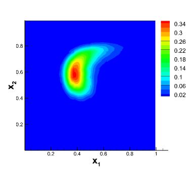
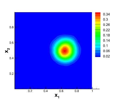
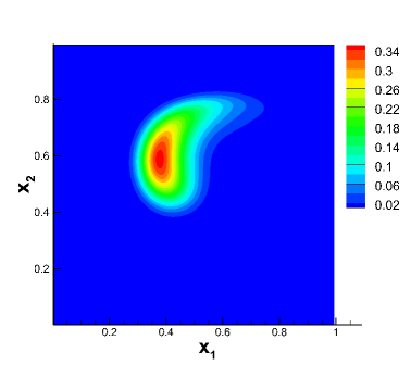
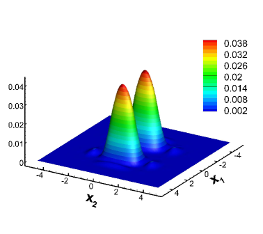
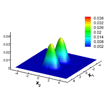
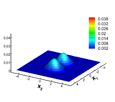
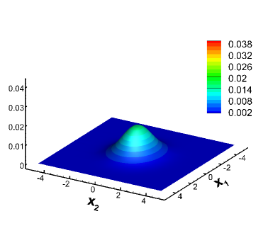
We still adopt the cosine bell (12) as the initial condition for this test, but with 𝐱c=(0.65,0.5)subscript𝐱𝑐0.650.5\mathbf{x}_{c}=(0.65,0.5) and b=0.35𝑏0.35b=0.35. Note that the deformational test is more challenging than the solid body rotation due to the space and time dependent flow field. In particular, along the direction of the flow, the cosine bell deforms into a crescent shape at t=T/2𝑡𝑇2t=T/2 , then goes back to its initial state at t=T𝑡𝑇t=T as the flow reverses. In the simulations, we compute the solution up to t=T𝑡𝑇t=T. The convergence study is summarized in Table 3. Similar order reduction is observed compared with Example 4.2. In Figure 1, we plot the contour plots of the numerical solutions at t=T/2𝑡𝑇2t=T/2 when the shape of the bell is greatly deformed, and t=T𝑡𝑇t=T when the solution is recovered into its initial state. It is observed that the sparse DG scheme with higher degree k𝑘k could better resolve the highly deformed solution structure.

Table 3: L2superscript𝐿2L^{2} errors and orders of accuracy for Example 4.3 at T=1.5𝑇1.5T=1.5. N𝑁N is the number of mesh levels, hNsubscript𝑁h_{N} is the size of the smallest mesh in each direction, k𝑘k is the polynomial order, d𝑑d is the dimension. DOF denotes the degrees of freedom of the sparse approximation space V^Nksubscriptsuperscript^𝑉𝑘𝑁\hat{V}^{k}_{N}. L2superscript𝐿2L^{2} order is calculated with respect to hNsubscript𝑁h_{N}. d=2𝑑2d=2.
N𝑁N hNsubscript𝑁h_{N} DOF L2superscript𝐿2L^{2} error order
k=1𝑘1k=1
5 1/32 448 1.40E-02
6 1/64 1024 6.88E-03 1.03
7 1/128 2304 2.65E-03 1.38
8 1/256 5120 8.48E-04 1.65
k=2𝑘2k=2
5 1/64 1008 3.32E-03
6 1/128 2304 1.31E-03 1.71
7 1/256 5184 3.82E-04 2.33
8 1/512 11520 5.92E-05 2.61
k=3𝑘3k=3
5 1/32 1792 6.28E-04
6 1/64 4096 1.22E-04 2.36
7 1/128 9216 1.37E-05 3.16
8 1/256 20480 2.02E-06 2.76
Refer to caption
Refer to caption
Refer to caption
Refer to caption
Refer to caption
Refer to caption
Fig. 1: Example 4.3. Deformational flow test. The contour plots of the numerical solutions at t=T/2𝑡𝑇2t=T/2 (a, c, e) and t=T𝑡𝑇t=T (b, d, f). k=1𝑘1k=1 (a, b), k=2𝑘2k=2 (c, d), and k=3𝑘3k=3 (e, f). N=7𝑁7N=7.

5 Kinetic simulations

In this section, we apply the sparse grid DG methods to solve kinetic equations. One of the major challenges for deterministic kinetic simulations is the high dimensionality of the underlying system. The unknown probability distribution function depends on the space and the velocity variables, which translates to numerical computation in six dimensions plus time in real-world settings. It is therefore a good test bed for sparse grid algorithms. In this paper, we focus on two types of kinetic systems: the collisionless Vlasov model and the collisional relaxation model. Both models are well understood in the literature and used as algorithm benchmarks. Our calculation will not involve solutions with discontinuity and numerical tests will be performed focusing on validating accuracy and conservation.

5.1 The collisionless Vlasov equation

In this subsection, we consider the non-dimensionalized single-species nonlinear Vlasov-Ampère system (VA) for plasma simulations in the zero-magnetic limit

ft+𝐯𝐱f+𝐄(t,𝐱)𝐯f=0,subscript𝑓𝑡𝐯subscript𝐱𝑓𝐄𝑡𝐱subscript𝐯𝑓0\displaystyle f_{t}+{\bf v}\cdot\nabla_{\mathbf{x}}f+\mathbf{E}(t,\mathbf{x})\cdot\nabla_{\bf v}f=0, (13)
t𝐄=𝐉,subscript𝑡𝐄𝐉\displaystyle\partial_{t}\mathbf{E}=-{\bf J}, (14)

where f(t,𝐱,𝐯)𝑓𝑡𝐱𝐯f(t,\mathbf{x},{\bf v}) denotes the probability distribution function of electrons. 𝐄(t,𝐱)𝐄𝑡𝐱\mathbf{E}(t,\mathbf{x}) is the self-consistent electrostatic field given by Ampère’s law (14) and 𝐉(t,𝐱)=𝐯f(t,𝐱,𝐯)𝐯𝑑𝐯𝐉𝑡𝐱subscript𝐯𝑓𝑡𝐱𝐯𝐯differential-d𝐯{\bf J}(t,\mathbf{x})=\int_{{\bf v}}f(t,\mathbf{x},{\bf v}){\bf v}d{\bf v} denotes the electron current density. Ions are assumed to form a neutralizing background. Note that the discussion here can be easily generalized to other popular Vlasov systems, such as Vlasov-Poisson or Vlasov-Maxwell systems.

The sparse grid DG method for the VA system can be formulated as follows. We solve the Vlasov equation by the algorithm discussed in previous sections, i.e. we compute fhsubscript𝑓f_{h} according to a similar formulation as in (2) treating the Vlasov equation as a variable coefficient transport problem, while the Ampère equation can be solved exactly, since 𝐉hsubscript𝐉{\bf J}_{h} is a piecewise polynomial supported on the discrete mesh in 𝐱𝐱\mathbf{x} and can be obtained exactly. In fact, the calculation of electron current 𝐉hsubscript𝐉{\bf J}_{h} is straightforward since 𝐯𝐯{\bf v} is orthogonal to all bases except those residing on level 0.00. The third order TVD-RK scheme is then used as the time discretization.

A focus of this work is to verify the conservation properties of the scheme. It is well known that the VA system preserves many physical invariants, including the particle number 𝐱𝐯f(t,𝐱,𝐯)𝑑𝐱𝑑𝐯,subscript𝐱subscript𝐯𝑓𝑡𝐱𝐯differential-d𝐱differential-d𝐯\int_{\mathbf{x}}\int_{\bf v}f(t,\mathbf{x},{\bf v})\,d\mathbf{x}d{\bf v}, total energy 12𝐱𝐯f(t,𝐱,𝐯)|𝐯|2𝑑𝐱𝑑𝐯+12𝐱|𝐄(t,𝐱)|2𝑑𝐱,12subscript𝐱subscript𝐯𝑓𝑡𝐱𝐯superscript𝐯2differential-d𝐱differential-d𝐯12subscript𝐱superscript𝐄𝑡𝐱2differential-d𝐱\frac{1}{2}\int_{\mathbf{x}}\int_{\bf v}f(t,\mathbf{x},{\bf v})|{\bf v}|^{2}\,d\mathbf{x}d{\bf v}+\frac{1}{2}\int_{\mathbf{x}}|\mathbf{E}(t,\mathbf{x})|^{2}\,d\mathbf{x}, and enstrophy 𝐱𝐯|f(t,𝐱,𝐯)|2𝑑𝐱𝑑𝐯.subscript𝐱subscript𝐯superscript𝑓𝑡𝐱𝐯2differential-d𝐱differential-d𝐯\int_{\mathbf{x}}\int_{\bf v}|f(t,\mathbf{x},{\bf v})|^{2}\,d\mathbf{x}d{\bf v}. Though it is difficult to design a numerical scheme which is able to preserve all the above invariants on the discrete level, tracking these quantities in time provides a good measurement for the performance of numerical schemes. Traditional DG methods were developed to solve the VA system [7] and superior performance in conservation of particle number and energy has been observed. As for the sparse grid DG method, we can easily verify similar properties for the semi-discrete scheme. The main reason is that the test function 111 and |𝐯|2superscript𝐯2|{\bf v}|^{2} used as the key steps in the proof of numerical conservation will still belong to the space 𝐕^Nksubscriptsuperscript^𝐕𝑘𝑁\hat{{\bf V}}^{k}_{N} as long as k2.𝑘2k\geq 2. In fact, they are functions that belong to the coarsest level of mesh.

Theorem 5.1 (Conservation properties).

Without the boundary effect, the semi-discrete sparse grid DG scheme for solving the VA system conserves the particle number. If k2𝑘2k\geq 2, the scheme also conserves the total energy. The scheme is L2superscript𝐿2L^{2} stable, i.e. ddt𝐱𝐯|fh(t,𝐱,𝐯)|2𝑑𝐱𝑑𝐯0.𝑑𝑑𝑡subscript𝐱subscript𝐯superscriptsubscript𝑓𝑡𝐱𝐯2differential-d𝐱differential-d𝐯0\frac{d}{dt}\int_{\mathbf{x}}\int_{\bf v}|f_{h}(t,\mathbf{x},{\bf v})|^{2}\,d\mathbf{x}d{\bf v}\leq 0.

The proof is similar to [8, 7] and is omitted. \blacksquare

Inspired by the theorem above, if one wants to design a DG scheme with particle number and energy conservation, it is enough to choose a basis set that includes 111 and |𝐯|2superscript𝐯2|{\bf v}|^{2} on level 00, while on other levels the bases can be chosen freely according to accuracy consideration. Such adaptivity is of interest to our future studies. In this paper, we consider the following two benchmark test cases in a 1D1V setting.

  • Landau damping:

    f(0,x,v)=fM(v)(1+Acos(kx)),x[0,L],v[Vc,Vc],formulae-sequence𝑓0𝑥𝑣subscript𝑓𝑀𝑣1𝐴𝑘𝑥formulae-sequence𝑥0𝐿𝑣subscript𝑉𝑐subscript𝑉𝑐f(0,x,v)=f_{M}(v)(1+A\cos(kx)),\quad x\in[0,L],\,v\in[-V_{c},V_{c}], (15)

    where A=0.5𝐴0.5A=0.5, k=0.5𝑘0.5k=0.5, L=4π𝐿4𝜋L=4\pi, Vc=2πsubscript𝑉𝑐2𝜋V_{c}=2\pi, and fM(v)=12πev2/2subscript𝑓𝑀𝑣12𝜋superscript𝑒superscript𝑣22f_{M}(v)=\frac{1}{\sqrt{2\pi}}e^{-v^{2}/2}.

  • Two-stream instability:

    f(0,x,v)=fTS(v)(1+Acos(kx)),x[0,L],v[Vc,Vc],formulae-sequence𝑓0𝑥𝑣subscript𝑓𝑇𝑆𝑣1𝐴𝑘𝑥formulae-sequence𝑥0𝐿𝑣subscript𝑉𝑐subscript𝑉𝑐f(0,x,v)=f_{TS}(v)(1+A\cos(kx)),\quad x\in[0,L],\,v\in[-V_{c},V_{c}], (16)

    where A=0.05𝐴0.05A=0.05, k=0.5𝑘0.5k=0.5, L=4π𝐿4𝜋L=4\pi, Vc=2πsubscript𝑉𝑐2𝜋V_{c}=2\pi, and fTS(v)=12πv2ev2/2subscript𝑓𝑇𝑆𝑣12𝜋superscript𝑣2superscript𝑒superscript𝑣22f_{TS}(v)=\frac{1}{\sqrt{2\pi}}v^{2}e^{-v^{2}/2}.

The periodic boundary condition is imposed in x𝑥x-space. As a standard practice, the computational domain in v𝑣v is truncated to [Vc,Vc]subscript𝑉𝑐subscript𝑉𝑐[-V_{c},V_{c}], where Vcsubscript𝑉𝑐V_{c} is a constant chosen large enough to impose zero boundary condition in the v𝑣v-direction fh(t,x,±Vc)=0.subscript𝑓𝑡𝑥plus-or-minussubscript𝑉𝑐0f_{h}(t,x,\pm V_{c})=0.

We first perform the accuracy test. Here we utilize the time reversibility of the VA system, i.e. if we let f(0,x,v)𝑓0𝑥𝑣f(0,x,v) be the initial condition and f(T,x,v)𝑓𝑇𝑥𝑣f(T,x,v) be the solution of the VA system at t=T𝑡𝑇t=T. When we reverse the velocity field of the solution, yielding f(T,x,v)𝑓𝑇𝑥𝑣f(T,x,-v), and evolve the VA system again to t=2T𝑡2𝑇t=2T, we would recover f(0,x,v)𝑓0𝑥𝑣f(0,x,-v), which is the initial condition with reverse velocity field. In our simulation, we use the sparse grid DG scheme to compute the solution to T=1𝑇1T=1 and then back to T=2𝑇2T=2, and compare it with the initial condition. The L2superscript𝐿2L^{2} errors and orders of accuracy are reported in Table 4. For both tests, we can observe slight order reduction from the optimal accuracy, which is similar to previous examples. The loss of accuracy for V^93superscriptsubscript^𝑉93\hat{V}_{9}^{3} for two-stream instability is due to the domain cut-off in the v𝑣v-space, which causes local truncation of about 108superscript10810^{-8}. This error can be reduced by taking a larger Vcsubscript𝑉𝑐V_{c}.

Table 4: L2superscript𝐿2L^{2} errors and orders of accuracy for the Vlasov-Ampère system. N𝑁N is the number of mesh levels, hNsubscript𝑁h_{N} is the size of the smallest mesh in each direction, k𝑘k is the polynomial order, d𝑑d is the dimension. DOF denotes the degrees of freedom of the sparse approximation space V^Nksubscriptsuperscript^𝑉𝑘𝑁\hat{V}^{k}_{N}. L2superscript𝐿2L^{2} order is calculated with respect to hNsubscript𝑁h_{N}. d=2𝑑2d=2.
N𝑁N hNsubscript𝑁h_{N} DOF L2superscript𝐿2L^{2} error order DOF L2superscript𝐿2L^{2} error order
Landau damping Two-stream instability
k=1𝑘1k=1 k=1𝑘1k=1
5 4π4𝜋4\pi/32 448 1.44E-01 448 2.77E-02
6 4π4𝜋4\pi/64 1024 5.71E-02 1.34 1024 7.37E-03 1.91
7 4π4𝜋4\pi/128 2304 1.17E-02 2.28 2304 2.12E-03 1.80
8 4π4𝜋4\pi/256 5120 3.07E-03 1.94 5120 5.89E-04 1.85
9 4π4𝜋4\pi/512 11264 8.01E-04 1.94 11264 1.52E-04 1.96
k=2𝑘2k=2 k=2𝑘2k=2
5 4π4𝜋4\pi/32 1008 1.03E-02 1008 2.58E-03
6 4π4𝜋4\pi/64 2304 3.07E-03 1.75 2304 3.89E-04 2.73
7 4π4𝜋4\pi/128 5184 4.62E-04 2.73 5184 6.13E-05 2.67
8 4π4𝜋4\pi/256 11520 1.09E-04 2.08 11520 9.66E-06 2.67
9 4π4𝜋4\pi/512 25344 1.86E-05 2.55 25344 1.59E-06 2.60
k=3𝑘3k=3 k=3𝑘3k=3
5 4π4𝜋4\pi/32 1792 1.95E-03 1792 1.52E-04
6 4π4𝜋4\pi/64 4096 4.26E-04 2.19 4096 1.15E-05 3.72
7 4π4𝜋4\pi/128 9216 3.54E-05 3.59 9216 8.82E-07 3.71
8 4π4𝜋4\pi/256 20480 4.44E-06 3.00 20480 5.89E-08 3.90
9 4π4𝜋4\pi/512 45056 2.65E-07 4.07 45056 3.56E-08 0.73

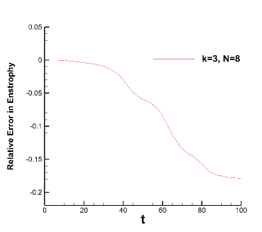
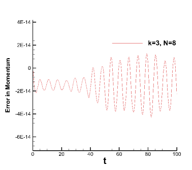
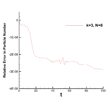
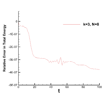
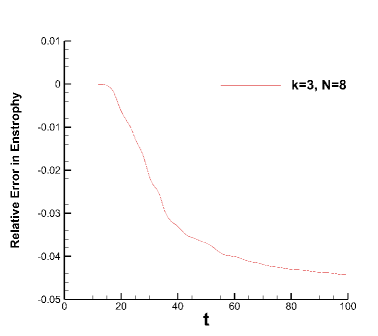
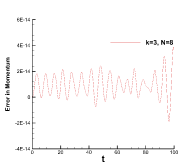
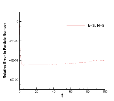
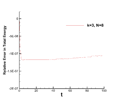
In Figures 2-3, we plot evolution of the relative error in the total particle number, total energy, and enstrophy, and evolution of error in momentum for the proposed method with sparse approximation space 𝐕^83superscriptsubscript^𝐕83\hat{{\bf V}}_{8}^{3}. For both cases, it is observed that the momentum are conserved up to machine error. The total particle number (f𝟏,𝟎𝟎superscriptsubscript𝑓100f_{\mathbf{1},{\mathbf{0}}}^{\mathbf{0}} in the code) is conserved up to the truncation errors at the boundary. Also note that even though the total energy is not conserved, the relative error is still on a quite small scale (107superscript10710^{-7}). This is due to the boundary effects and the errors from the Runge-Kutta schemes. The visible decay in enstrophy is expected because of the dissipative upwind flux.
Refer to caption
Refer to caption
Refer to caption
Refer to caption
Fig. 2: Landau damping. Evolution of the relative errors in total particle number (a), total energy (b), entrophy (c), and evolution of error in momentum (d). k=3𝑘3k=3, N=8𝑁8N=8.
Refer to caption
Refer to caption
Refer to caption
Refer to caption
Fig. 3: Two-stream instability. Evolution of the relative errors in total particle number (a), total energy (b), entrophy (c), and evolution of error in momentum (d). k=3𝑘3k=3, N=8𝑁8N=8.

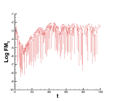
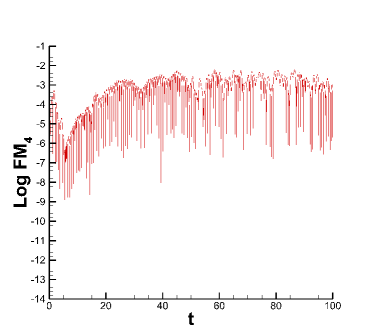
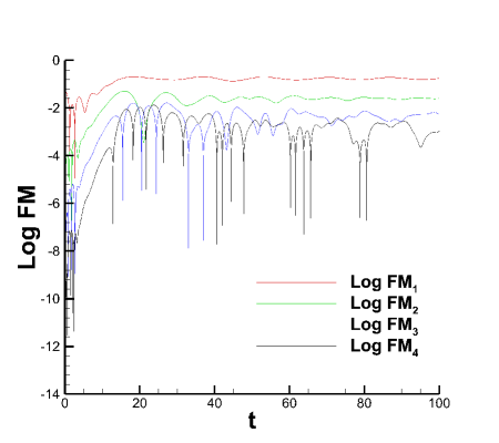
We further present some numerical data to benchmark the proposed scheme. We first consider the Log Fourier modes of the electric field E(t,x)𝐸𝑡𝑥E(t,x) as functions of time, which are defined as

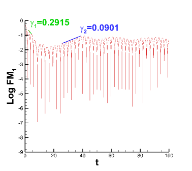
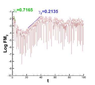
logFMn(t)=log10(1L|0LE(t,x)sin(knx)𝑑x|2+|0LE(t,x)cos(knx)𝑑x|2).𝐹subscript𝑀𝑛𝑡subscript101𝐿superscriptsuperscriptsubscript0𝐿𝐸𝑡𝑥𝑘𝑛𝑥differential-d𝑥2superscriptsuperscriptsubscript0𝐿𝐸𝑡𝑥𝑘𝑛𝑥differential-d𝑥2\log FM_{n}(t)=\log_{10}\left(\frac{1}{L}\sqrt{\left|\int_{0}^{L}E(t,x)\,\sin(knx)\,dx\right|^{2}+\left|\int_{0}^{L}E(t,x)\,\cos(knx)\,dx\right|^{2}}\right).

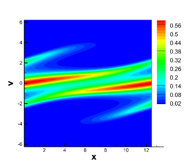
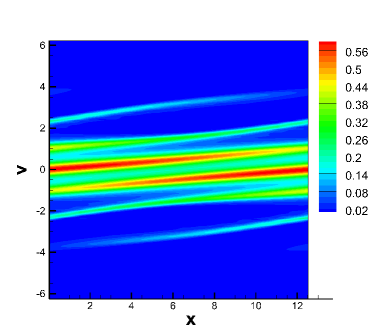
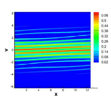
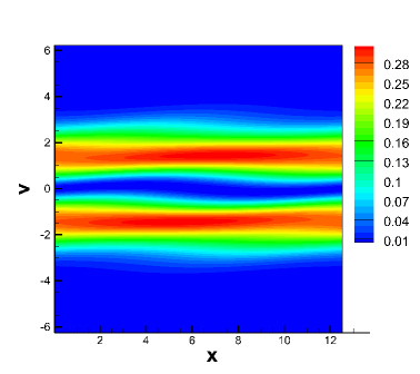
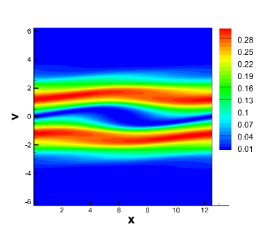
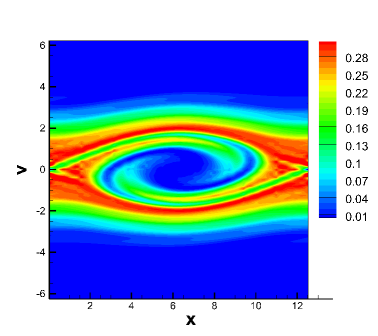
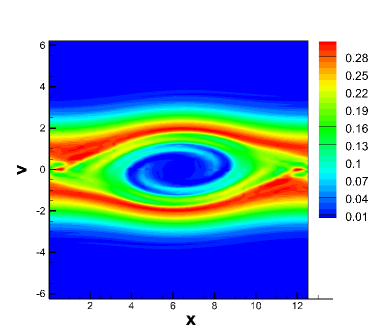
In Figures 4-5, we show the time evolution of the first four Log Fourier modes when simulating Landau damping and two-stream instability, respectively. The sparse approximation space 𝐕^83superscriptsubscript^𝐕83\hat{{\bf V}}_{8}^{3} is used in our computation. The results agree with other calculations in the literature. In Figures 6-7, we present the phase space contour plots at several instances of time for Landau damping and two stream instability computed with space 𝐕^83superscriptsubscript^𝐕83\hat{{\bf V}}_{8}^{3}. Note that the number of degrees of freedom of used sparse approximation space is relatively small (which is 20480), yet those numerical results agree with the benchmarks in the literature.
Refer to caption
Refer to caption
Refer to caption
Refer to caption
Fig. 4: The first four log Fourier modes of Landau damping. k=3𝑘3k=3, N=8𝑁8N=8.
Refer to caption
Fig. 5: The first four log Fourier modes of two-stream instability. k=3𝑘3k=3, N=8𝑁8N=8.
Refer to caption
Refer to caption
Refer to caption
Refer to caption
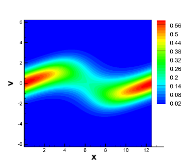
Fig. 6: Landau damping. Phase space contour plots at t=1𝑡1t=1 (a), t=5𝑡5t=5 (b), t=10𝑡10t=10 (c), and t=20𝑡20t=20 (d). k=3𝑘3k=3, N=8𝑁8N=8.
Refer to caption
Refer to caption
Refer to caption
Refer to caption
Fig. 7: Two-stream instability. Phase space contour plots at t=5𝑡5t=5 (a), t=10𝑡10t=10 (b), t=20𝑡20t=20 (c), and t=40𝑡40t=40 (d). k=3𝑘3k=3, N=8𝑁8N=8.

5.2 The relaxation model

The last example we present in this paper is the linear Vlasov-Boltzmann transport equation

ft+𝐯𝐱f+𝐄(t,𝐱)𝐯f=L(f),subscript𝑓𝑡𝐯subscript𝐱𝑓𝐄𝑡𝐱subscript𝐯𝑓𝐿𝑓f_{t}+{\bf v}\cdot\nabla_{\mathbf{x}}f+\mathbf{E}(t,\mathbf{x})\cdot\nabla_{\bf v}f=L(f), (17)

where L(f)𝐿𝑓L(f) denotes the linear relaxation operator

L(f)=μ(𝐯)ρ(t,𝐱)f(t,𝐱,𝐯)τ,𝐿𝑓subscript𝜇𝐯𝜌𝑡𝐱𝑓𝑡𝐱𝐯𝜏L(f)=\frac{\mu_{\infty}({\bf v})\rho(t,\mathbf{x})-f(t,\mathbf{x},{\bf v})}{\tau},

and μ(𝐯)subscript𝜇𝐯\mu_{\infty}({\bf v}) is an absolute Maxwellian distribution defined as

μ(𝐯)=exp(|𝐯|22θ)(2πθ)d/2,subscript𝜇𝐯superscript𝐯22𝜃superscript2𝜋𝜃𝑑2\mu_{\infty}({\bf v})=\frac{\exp(-\frac{|{\bf v}|^{2}}{2\theta})}{(2\pi\theta)^{d/2}},

and

ρ(t,𝐱)=𝐯f(t,𝐱,𝐯)𝑑𝐯𝜌𝑡𝐱subscript𝐯𝑓𝑡𝐱𝐯differential-d𝐯\rho(t,\mathbf{x})=\int_{{\bf v}}f(t,\mathbf{x},{\bf v})\,d{\bf v}

denotes the macroscopic density. The external electric field 𝐄(t,𝐱)𝐄𝑡𝐱\mathbf{E}(t,\mathbf{x}) is given by a known electrostatic potential

𝐄(𝐱)=𝐱Φ(𝐱)withΦ(x)=|𝐱|22.formulae-sequence𝐄𝐱subscript𝐱Φ𝐱withΦ𝑥superscript𝐱22\mathbf{E}(\mathbf{x})=-\nabla_{\mathbf{x}}\Phi(\mathbf{x})\quad\text{with}\quad\Phi(x)=\frac{|\mathbf{x}|^{2}}{2}.

In this case, the unique stationary state solution (𝐱,𝐯)𝐱𝐯\mathcal{M}(\mathbf{x},{\bf v}) of equation (17) is the global Maxwellian distribution μ(𝐯)subscript𝜇𝐯\mu_{\infty}({\bf v}) multiplied by the stationary macroscopic density given by the spatial Maxwellian

ρ(𝐱)=exp(Φ(𝐱)/θ)𝐱exp(Φ(𝐱)/θ)𝑑𝐱,subscript𝜌𝐱Φ𝐱𝜃subscript𝐱Φ𝐱𝜃differential-d𝐱\rho_{\infty}(\mathbf{x})=\frac{\exp(-\Phi(\mathbf{x})/\theta)}{\int_{\mathbf{x}}\exp(-\Phi(\mathbf{x})/\theta)\,d\mathbf{x}},

i.e.,

(𝐱,𝐯)=ρ(𝐱)μ(𝐯)=exp((|𝐯|22+Φ(𝐱))/θ)(2πθ)d/2𝐱exp(Φ(𝐱)/θ)𝑑𝐱.𝐱𝐯subscript𝜌𝐱subscript𝜇𝐯superscript𝐯22Φ𝐱𝜃superscript2𝜋𝜃𝑑2subscript𝐱Φ𝐱𝜃differential-d𝐱\mathcal{M}(\mathbf{x},{\bf v})=\rho_{\infty}(\mathbf{x})\mu_{\infty}({\bf v})=\frac{\exp\left(-\left(\frac{|{\bf v}|^{2}}{2}+\Phi(\mathbf{x})\right)/\theta\right)}{(2\pi\theta)^{d/2}\int_{\mathbf{x}}\exp(-\Phi(\mathbf{x})/\theta)\,d\mathbf{x}}.

A DG scheme with traditional piecewise polynomial space for (17) has been developed and analyzed in [10]. Here, we use the sparse DG scheme to solve the problem (17) in a cut-off domain Ω=[L,L]d×[Vc,Vc]dΩsuperscript𝐿𝐿𝑑superscriptsubscript𝑉𝑐subscript𝑉𝑐𝑑\Omega=[-L,L]^{d}\times[-V_{c},V_{c}]^{d} with d=1, 2𝑑12d=1,\,2 (two dimensional and four dimensional calculations, resp.). The following initial conditions are used:

f(0,𝐱,𝐯)𝑓0𝐱𝐯\displaystyle f(0,\mathbf{x},{\bf v}) =1s1sin(x2/2)2exp((x2+v2)/2),whend=1,\displaystyle=\frac{1}{s_{1}}\sin(x^{2}/2)^{2}\exp(-(x^{2}+v^{2})/2),\quad\text{when}\quad d=1,
f(0,𝐱,𝐯)𝑓0𝐱𝐯\displaystyle f(0,\mathbf{x},{\bf v}) =1s2sin(x12/2)2cos(x22/2)2exp((x12+x22+v12+v22)/2),whend=2,\displaystyle=\frac{1}{s_{2}}\sin(x_{1}^{2}/2)^{2}\cos(x_{2}^{2}/2)^{2}\exp(-(x_{1}^{2}+x_{2}^{2}+v_{1}^{2}+v_{2}^{2})/2),\quad\text{when}\quad d=2,

where s1,s2subscript𝑠1subscript𝑠2s_{1},\,s_{2} are normalization constants such that Ωf(0,𝐱,𝐯)𝑑𝐱𝑑𝐯=1subscriptΩ𝑓0𝐱𝐯differential-d𝐱differential-d𝐯1\int_{\Omega}f(0,\mathbf{x},{\bf v})d\mathbf{x}d{\bf v}=1. The zero boundary conditions are imposed in both 𝐱limit-from𝐱\mathbf{x}- and 𝐯limit-from𝐯{\bf v}-spaces. We take Vc=5subscript𝑉𝑐5V_{c}=5, and τ=θ=1𝜏𝜃1\tau=\theta=1.

For the case of d=1𝑑1d=1, we investigate the decay rate of the initial state to equilibrium by tracking time evolution of the following two entropy functionals

log(t)=ΩHlog(H)𝑑x𝑑v,2(t)=ΩH2𝑑x𝑑v,formulae-sequencesubscript𝑙𝑜𝑔𝑡subscriptΩ𝐻𝐻differential-d𝑥differential-d𝑣subscript2𝑡subscriptΩsuperscript𝐻2differential-d𝑥differential-d𝑣\mathcal{H}_{log}(t)=\int_{\Omega}H\log(H)\mathcal{M}\,dxdv,\quad\mathcal{H}_{2}(t)=\int_{\Omega}H^{2}\mathcal{M}\,dxdv,

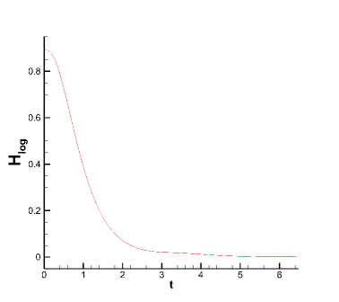
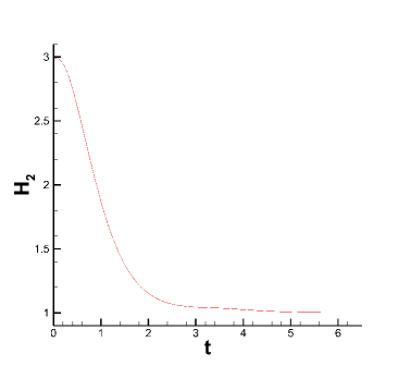
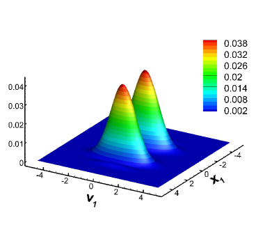
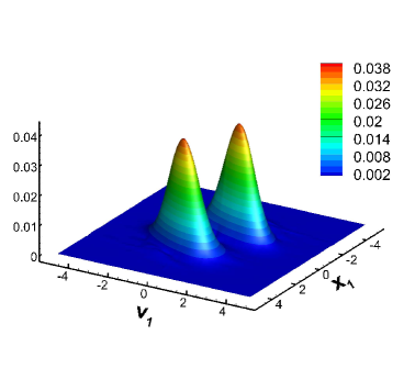
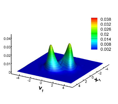
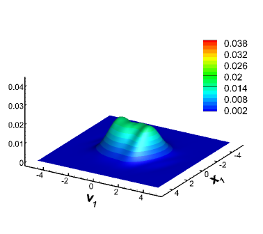
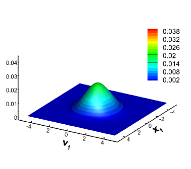
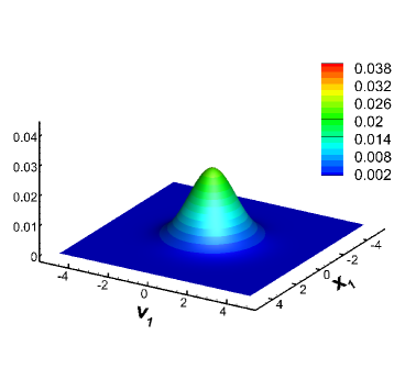
where H(t,x,v)=fh/𝐻𝑡𝑥𝑣subscript𝑓H(t,x,v)=f_{h}/\mathcal{M} is the global relative entropy function. logsubscript𝑙𝑜𝑔\mathcal{H}_{log} and 2subscript2\mathcal{H}_{2} should relax to 00 and 111 indicating convergence to equilibrium. In the simulation, we use the sparse DG scheme with 𝐕^73subscriptsuperscript^𝐕37\hat{{\bf V}}^{3}_{7} and plot the decay rate with respect to both entropy functionals in Figure 8. Both plots verify the convergence of numerical solution to .\mathcal{M}. For the case of d=2𝑑2d=2, the sparse DG method with approximation space 𝐕^83subscriptsuperscript^𝐕38\hat{{\bf V}}^{3}_{8} is used. In Figures 9-10, we report the evolution of the two-dimensional cuts in x1v1subscript𝑥1subscript𝑣1x_{1}-v_{1} plane at x2=0,v2=0formulae-sequencesubscript𝑥20subscript𝑣20x_{2}=0,\,v_{2}=0 and in x1x2subscript𝑥1subscript𝑥2x_{1}-x_{2} plane at v1=0,v2=0formulae-sequencesubscript𝑣10subscript𝑣20v_{1}=0,\,v_{2}=0. Similar to the case of d=1𝑑1d=1, fhsubscript𝑓f_{h} in both two-dimensional cuts is observed to relax towards the equilibrium distribution \mathcal{M}.

Refer to caption
Refer to caption
Fig. 8: Linear Vlasov-Boltzmann equation. Decay rate for entropy functional logsubscript𝑙𝑜𝑔\mathcal{H}_{log} (a) and 2subscript2\mathcal{H}_{2} (b). k=3𝑘3k=3, N=7𝑁7N=7, d=1𝑑1d=1.
Refer to caption
Refer to caption
Refer to caption
Refer to caption
Refer to caption
Refer to caption
Fig. 9: Linear Vlasov-Boltzmann equation. The two-dimensional cuts in x1v1subscript𝑥1subscript𝑣1x_{1}-v_{1} plane of the evolution of fhsubscript𝑓f_{h} towards equilibrium at x2=0subscript𝑥20x_{2}=0 and v2=0subscript𝑣20v_{2}=0. t=0𝑡0t=0 (a), t=0.5𝑡0.5t=0.5 (b), t=1𝑡1t=1 (c), t=2𝑡2t=2 (d), t=3𝑡3t=3 (e), and t=6𝑡6t=6 (f). k=3𝑘3k=3, N=8𝑁8N=8, d=2𝑑2d=2.
Refer to caption
Refer to caption
Refer to caption
Refer to caption
Refer to caption
Refer to caption
Fig. 10: Linear Vlasov-Boltzmann equation. The two-dimensional cuts in x1x2subscript𝑥1subscript𝑥2x_{1}-x_{2} plane at v1=0subscript𝑣10v_{1}=0 and v2=0subscript𝑣20v_{2}=0 of the evolution of fhsubscript𝑓f_{h} towards equilibrium. t=0𝑡0t=0 (a), t=0.5𝑡0.5t=0.5 (b), t=1𝑡1t=1 (c), t=2𝑡2t=2 (d), t=3𝑡3t=3 (e), and t=6𝑡6t=6 (f). k=3𝑘3k=3, N=8𝑁8N=8, d=2𝑑2d=2.

6 Conclusions and future work

In this paper, we developed a sparse grid DG scheme for variable-coefficient transport equations. The method uses a sparse finite element space based on a hierarchical construction of basis functions and are shown to reduce the computational degrees of freedom significantly in high dimensions. Weak formulations of traditional DG methods are incorporated ensuring many nice properties such as conservation and stability. For constant coefficient equations, we established semi-discrete L2superscript𝐿2L^{2} stability and error estimate of order O((logh)dhk+1/2)𝑂superscript𝑑superscript𝑘12O((\log h)^{d}h^{k+1/2}) for smooth enough solutions where hh is the size of the finest mesh in each dimension. The method is applied to kinetic simulations of Vlasov and Boltzmann equations. Good performance in accuracy and conservation is observed. Future work includes further investigation of error estimates in various norms, and development of the scheme for solutions with less regularities.

Appendix A Proof of Lemma 3.2

In this appendix, we prove the approximation results of Lemma 3.2 in three steps. Many discussions are closely related to [22], where the C0superscript𝐶0C^{0} sparse finite element space was considered. The main difference lies in the splitting of the errors into two parts to fine tune the estimates for discontinuous piecewise polynomials in 𝐕^Nksuperscriptsubscript^𝐕𝑁𝑘\hat{{\bf V}}_{N}^{k}.

A.1 An alternative representation of the L2superscript𝐿2L^{2} projection

To facilitate the discussion, we seek an alternative representation of the L2superscript𝐿2L^{2} projection 𝐏𝐏\mathbf{P} onto 𝐕^Nksuperscriptsubscript^𝐕𝑁𝑘\hat{{\bf V}}_{N}^{k} following a similar construction in [22]. We denote Pnksuperscriptsubscript𝑃𝑛𝑘P_{n}^{k} as the standard L2superscript𝐿2L^{2} projection operator from L2(0,1)superscript𝐿201L^{2}(0,1) to Vnksuperscriptsubscript𝑉𝑛𝑘V_{n}^{k}, and the induced increment projector

Qnk:={PnkPn1k,ifn1,P0k,ifn=0,assignsuperscriptsubscript𝑄𝑛𝑘casessuperscriptsubscript𝑃𝑛𝑘superscriptsubscript𝑃𝑛1𝑘if𝑛1superscriptsubscript𝑃0𝑘if𝑛0Q_{n}^{k}:=\left\{\begin{array}[]{ll}P_{n}^{k}-P_{n-1}^{k},&\textrm{if}\,n\geq 1,\\ P_{0}^{k},&\textrm{if}\,n=0,\end{array}\right.

and further denote

𝐏^Nk:=|𝐥|1N𝐥0dQl1,x1kQld,xdk,assignsuperscriptsubscript^𝐏𝑁𝑘subscriptsubscript𝐥1𝑁𝐥superscriptsubscript0𝑑tensor-productsubscriptsuperscript𝑄𝑘subscript𝑙1subscript𝑥1subscriptsuperscript𝑄𝑘subscript𝑙𝑑subscript𝑥𝑑\hat{{\bf P}}_{N}^{k}:=\sum_{\begin{subarray}{c}|\mathbf{l}|_{1}\leq N\\ \mathbf{l}\in\mathbb{N}_{0}^{d}\end{subarray}}{Q}^{k}_{l_{1},x_{1}}\otimes\cdots\otimes{Q}^{k}_{l_{d},x_{d}}, (18)

where the second subindex of Qli,xiksubscriptsuperscript𝑄𝑘subscript𝑙𝑖subscript𝑥𝑖{Q}^{k}_{l_{i},x_{i}} indicates that the increment operator is defined in xisubscript𝑥𝑖x_{i}-direction. We can easily show that 𝐏=𝐏^Nk.𝐏superscriptsubscript^𝐏𝑁𝑘{\bf P}=\hat{{\bf P}}_{N}^{k}. In fact, for any v𝑣v, it’s clear that 𝐏^Nkv𝐕^Nksuperscriptsubscript^𝐏𝑁𝑘𝑣superscriptsubscript^𝐕𝑁𝑘\hat{{\bf P}}_{N}^{k}v\in\hat{{\bf V}}_{N}^{k}. Therefore, we only need

Ω(𝐏^Nkvv)w𝑑𝐱=0,w𝐕^Nk.formulae-sequencesubscriptΩsuperscriptsubscript^𝐏𝑁𝑘𝑣𝑣𝑤differential-d𝐱0for-all𝑤superscriptsubscript^𝐕𝑁𝑘\int_{\Omega}(\hat{{\bf P}}_{N}^{k}v-v)w\,d\mathbf{x}=0,\qquad\forall\,w\in\hat{{\bf V}}_{N}^{k}. (19)

It suffices to show (19) for vC(Ω)𝑣superscript𝐶Ωv\in C^{\infty}(\Omega) which is a dense subset of L2(Ω)superscript𝐿2ΩL^{2}(\Omega). In fact, we have

v=𝐥0dQl1,x1kQld,xdkv.𝑣subscript𝐥superscriptsubscript0𝑑tensor-productsubscriptsuperscript𝑄𝑘subscript𝑙1subscript𝑥1subscriptsuperscript𝑄𝑘subscript𝑙𝑑subscript𝑥𝑑𝑣v=\sum_{\mathbf{l}\in\mathbb{N}_{0}^{d}}{Q}^{k}_{l_{1},x_{1}}\otimes\cdots\otimes{Q}^{k}_{l_{d},x_{d}}v.

Therefore,

Ω(𝐏^Nkvv)w𝑑𝐱=Ω(|𝐥|1>N𝐥0dQl1,x1kQld,xdkv)w𝑑𝐱.subscriptΩsuperscriptsubscript^𝐏𝑁𝑘𝑣𝑣𝑤differential-d𝐱subscriptΩsubscriptsubscript𝐥1𝑁𝐥superscriptsubscript0𝑑tensor-productsubscriptsuperscript𝑄𝑘subscript𝑙1subscript𝑥1subscriptsuperscript𝑄𝑘subscript𝑙𝑑subscript𝑥𝑑𝑣𝑤differential-d𝐱\int_{\Omega}(\hat{{\bf P}}_{N}^{k}v-v)w\,d\mathbf{x}=\int_{\Omega}(\sum_{\begin{subarray}{c}|\mathbf{l}|_{1}>N\\ \mathbf{l}\in\mathbb{N}_{0}^{d}\end{subarray}}{Q}^{k}_{l_{1},x_{1}}\otimes\cdots\otimes{Q}^{k}_{l_{d},x_{d}}v)\,w\,d\mathbf{x}. (20)

Since the one dimensional projectors satisfy

[0,1]Qnkϕφ𝑑x=0,φVn1k,formulae-sequencesubscript01superscriptsubscript𝑄𝑛𝑘italic-ϕ𝜑differential-d𝑥0𝜑superscriptsubscript𝑉𝑛1𝑘\int_{[0,1]}Q_{n}^{k}\phi\,\varphi\,dx=0,\quad\varphi\in V_{n-1}^{k},

for any n1,ϕL2(0,1).formulae-sequence𝑛1italic-ϕsuperscript𝐿201n\geq 1,\phi\in L^{2}(0,1). (20) is immediate from the definition of the tensor-product operators and we are done.

A.2 Properties of the one-dimensional and tensor product projections

Here, we review some classical approximation results about the one-dimensional projection Pnksuperscriptsubscript𝑃𝑛𝑘P_{n}^{k} and their tensor-product constructions.

Property A.1 (Convergence property of the 1D projections [11]).

For a function vHp+1(0,1)𝑣superscript𝐻𝑝101v\in H^{p+1}(0,1), we have the convergence property of the L2superscript𝐿2L^{2} projection Pnksuperscriptsubscript𝑃𝑛𝑘P_{n}^{k} as follows: for any integer t𝑡t with 1qmin{p,k}1𝑞𝑝𝑘1\leq q\leq\min\{p,k\}, s=0, 1𝑠01s=0,\,1,

|Pnkvv|Hs(Inj)ck,s,q2n(q+1s)|v|Hq+1(Inj),j=0,,2n+11,formulae-sequencesubscriptsuperscriptsubscript𝑃𝑛𝑘𝑣𝑣superscript𝐻𝑠subscriptsuperscript𝐼𝑗𝑛subscript𝑐𝑘𝑠𝑞superscript2𝑛𝑞1𝑠subscript𝑣superscript𝐻𝑞1subscriptsuperscript𝐼𝑗𝑛𝑗0superscript2𝑛11|P_{n}^{k}v-v|_{H^{s}(I^{j}_{n})}\leq c_{k,s,q}2^{-n(q+1-s)}|v|_{H^{q+1}(I^{j}_{n})},\quad j=0,\cdots,2^{n+1}-1, (21)

where ck,s,qsubscript𝑐𝑘𝑠𝑞c_{k,s,q} is a constant that depends on k,s,q𝑘𝑠𝑞k,s,q, but not on n𝑛n, and the case of s=0𝑠0s=0 refers to the L2superscript𝐿2L^{2} norm.

From this property, using basic algebra, we can deduce that for n1𝑛1n\geq 1,

|Qnkv|Hs(Inj)c~k,s,q2n(q+1s)|v|Hq+1(Inj),subscriptsuperscriptsubscript𝑄𝑛𝑘𝑣superscript𝐻𝑠subscriptsuperscript𝐼𝑗𝑛subscript~𝑐𝑘𝑠𝑞superscript2𝑛𝑞1𝑠subscript𝑣superscript𝐻𝑞1subscriptsuperscript𝐼𝑗𝑛|Q_{n}^{k}v|_{H^{s}(I^{j}_{n})}\leq\tilde{c}_{k,s,q}2^{-n(q+1-s)}|v|_{H^{q+1}(I^{j}_{n})}, (22)

with

c~k,s,q=ck,s,q(1+2(q+1s)).subscript~𝑐𝑘𝑠𝑞subscript𝑐𝑘𝑠𝑞1superscript2𝑞1𝑠\tilde{c}_{k,s,q}=c_{k,s,q}\,(1+2^{-(q+1-s)}). (23)

When n=0𝑛0n=0, first note that the L2superscript𝐿2L^{2} projector Q0k=P0ksuperscriptsubscript𝑄0𝑘superscriptsubscript𝑃0𝑘Q_{0}^{k}=P_{0}^{k} preserves the L2superscript𝐿2L^{2} norm, i.e.,

Q0kvL2(0,1)=vL2(0,1).subscriptnormsuperscriptsubscript𝑄0𝑘𝑣superscript𝐿201subscriptnorm𝑣superscript𝐿201\|Q_{0}^{k}v\|_{L^{2}(0,1)}=\|v\|_{L^{2}(0,1)}.

Moreover, by the inverse inequality, see, e.g., [21], we have

|Q0kv|H1(0,1)cinvkQ0kvL2(0,1)=cinvkvL2(0,1),subscriptsuperscriptsubscript𝑄0𝑘𝑣superscript𝐻101subscriptsuperscript𝑐𝑘𝑖𝑛𝑣subscriptnormsuperscriptsubscript𝑄0𝑘𝑣superscript𝐿201subscriptsuperscript𝑐𝑘𝑖𝑛𝑣subscriptnorm𝑣superscript𝐿201|Q_{0}^{k}v|_{H^{1}(0,1)}\leq c^{k}_{inv}\|Q_{0}^{k}v\|_{L^{2}(0,1)}=c^{k}_{inv}\|v\|_{L^{2}(0,1)},

where cinvk=12k2.subscriptsuperscript𝑐𝑘𝑖𝑛𝑣12superscript𝑘2c^{k}_{inv}=\sqrt{12}k^{2}. Therefore, we have obtained the following estimation

|Q0kv|Hs(0,1)c^k,svL2(0,1),s=0, 1,formulae-sequencesubscriptsuperscriptsubscript𝑄0𝑘𝑣superscript𝐻𝑠01subscript^𝑐𝑘𝑠subscriptnorm𝑣superscript𝐿201𝑠01|Q_{0}^{k}v|_{H^{s}(0,1)}\leq\hat{c}_{k,s}\|v\|_{L^{2}(0,1)},\quad s=0,\,1, (24)

where c^k,0=1subscript^𝑐𝑘01\hat{c}_{k,0}=1 and c^k,1=cinvksubscript^𝑐𝑘1superscriptsubscript𝑐𝑖𝑛𝑣𝑘\hat{c}_{k,1}=c_{inv}^{k}.

For multi-dimensions, if we consider the L2superscript𝐿2L^{2} projection 𝐏Nk=PN,x1kPN,xdksubscriptsuperscript𝐏𝑘𝑁tensor-productsubscriptsuperscript𝑃𝑘𝑁subscript𝑥1subscriptsuperscript𝑃𝑘𝑁subscript𝑥𝑑{\bf P}^{k}_{N}={P}^{k}_{N,x_{1}}\otimes\cdots\otimes{P}^{k}_{N,x_{d}} onto the standard piecewise polynomial space 𝐕Nksuperscriptsubscript𝐕𝑁𝑘{\bf V}_{N}^{k}, we have the following approximation results.

Property A.2 (Convergence property of the multi-dimensional tensor-product projectors [11]).

For a function vHp+1(Ω)𝑣superscript𝐻𝑝1Ωv\in H^{p+1}(\Omega), we have the convergence property of the L2superscript𝐿2L^{2} projection 𝐏Nksubscriptsuperscript𝐏𝑘𝑁{\bf P}^{k}_{N} onto 𝐕Nksuperscriptsubscript𝐕𝑁𝑘{\bf V}_{N}^{k} as follows: for any integer t𝑡t with 1qmin{p,k}1𝑞𝑝𝑘1\leq q\leq\min\{p,k\}, s=0, 1𝑠01s=0,\,1,

|𝐏Nkvv|Hs(ΩN)c¯¯k,s,q2N(q+1s)|v|Hq+1(Ω),subscriptsuperscriptsubscript𝐏𝑁𝑘𝑣𝑣superscript𝐻𝑠subscriptΩ𝑁subscript¯¯𝑐𝑘𝑠𝑞superscript2𝑁𝑞1𝑠subscript𝑣superscript𝐻𝑞1Ω|{\bf P}_{N}^{k}v-v|_{H^{s}(\Omega_{N})}\leq\bar{\bar{c}}_{k,s,q}2^{-N(q+1-s)}|v|_{H^{q+1}(\Omega)}, (25)

where c¯¯k,s,qsubscript¯¯𝑐𝑘𝑠𝑞\bar{\bar{c}}_{k,s,q} is a constant that depends on k,s,q𝑘𝑠𝑞k,s,q, but not on N𝑁N.

A.3 Proof of Lemma 3.2

In this subsection, we will prove Lemma 3.2. For any function vL2(Ω)𝑣superscript𝐿2Ωv\in L^{2}(\Omega), we split the error into two parts as follows,

v𝐏v=v𝐏^Nkv=v𝐏Nkv+𝐏Nkv𝐏^Nkv.𝑣𝐏𝑣𝑣superscriptsubscript^𝐏𝑁𝑘𝑣𝑣subscriptsuperscript𝐏𝑘𝑁𝑣subscriptsuperscript𝐏𝑘𝑁𝑣superscriptsubscript^𝐏𝑁𝑘𝑣v-{\bf P}v=v-{\hat{{\bf P}}}_{N}^{k}v=v-{\bf P}^{k}_{N}v+{\bf P}^{k}_{N}v-{\hat{{\bf P}}}_{N}^{k}v.

The term v𝐏Nkv𝑣superscriptsubscript𝐏𝑁𝑘𝑣v-{\bf P}_{N}^{k}v can be estimated by Property A.2. Therefore we only need to bound

𝐏Nkv𝐏^Nkvsubscriptsuperscript𝐏𝑘𝑁𝑣superscriptsubscript^𝐏𝑁𝑘𝑣\displaystyle{\bf P}^{k}_{N}v-{\hat{{\bf P}}}_{N}^{k}v =|𝐥|N𝐥0dQl1,x1kQld,xdkv|𝐥|1N𝐥0dQl1,x1kQld,xdkvabsentsubscriptsubscript𝐥𝑁𝐥superscriptsubscript0𝑑tensor-productsubscriptsuperscript𝑄𝑘subscript𝑙1subscript𝑥1subscriptsuperscript𝑄𝑘subscript𝑙𝑑subscript𝑥𝑑𝑣subscriptsubscript𝐥1𝑁𝐥superscriptsubscript0𝑑tensor-productsubscriptsuperscript𝑄𝑘subscript𝑙1subscript𝑥1subscriptsuperscript𝑄𝑘subscript𝑙𝑑subscript𝑥𝑑𝑣\displaystyle=\sum_{\begin{subarray}{c}|\mathbf{l}|_{\infty}\leq N\\ \mathbf{l}\in\mathbb{N}_{0}^{d}\end{subarray}}{Q}^{k}_{l_{1},x_{1}}\otimes\cdots\otimes{Q}^{k}_{l_{d},x_{d}}v-\sum_{\begin{subarray}{c}|\mathbf{l}|_{1}\leq N\\ \mathbf{l}\in\mathbb{N}_{0}^{d}\end{subarray}}{Q}^{k}_{l_{1},x_{1}}\otimes\cdots\otimes{Q}^{k}_{l_{d},x_{d}}v
=|𝐥|N,|𝐥|1>N𝐥0dQl1,x1kQld,xdkv.absentsubscriptformulae-sequencesubscript𝐥𝑁subscript𝐥1𝑁𝐥superscriptsubscript0𝑑tensor-productsubscriptsuperscript𝑄𝑘subscript𝑙1subscript𝑥1subscriptsuperscript𝑄𝑘subscript𝑙𝑑subscript𝑥𝑑𝑣\displaystyle=\sum_{\begin{subarray}{c}|\mathbf{l}|_{\infty}\leq N,|\mathbf{l}|_{1}>N\\ \mathbf{l}\in\mathbb{N}_{0}^{d}\end{subarray}}{Q}^{k}_{l_{1},x_{1}}\otimes\cdots\otimes{Q}^{k}_{l_{d},x_{d}}v.

In what follows, we will estimate the tensor-product construction of increment projections when |𝐥|N,|𝐥|1>Nformulae-sequencesubscript𝐥𝑁subscript𝐥1𝑁|\mathbf{l}|_{\infty}\leq N,|\mathbf{l}|_{1}>N. Assume up+1(Ω)𝑢superscript𝑝1Ωu\in\mathcal{H}^{p+1}(\Omega), and q𝑞q is an integer with 1qmin{p,k}.1𝑞𝑝𝑘1\leq q\leq\min\{p,k\}. For a multi-index 𝐥𝐥\mathbf{l} with |𝐥|N,|𝐥|1>Nformulae-sequencesubscript𝐥𝑁subscript𝐥1𝑁|\mathbf{l}|_{\infty}\leq N,|\mathbf{l}|_{1}>N, let L=supp(𝐥):={i1,i2,,ir}{1,2,,d}𝐿𝑠𝑢𝑝𝑝𝐥assignsubscript𝑖1subscript𝑖2subscript𝑖𝑟12𝑑L=supp(\mathbf{l}):=\{i_{1},i_{2},\cdots,i_{r}\}\subset\{1,2,\cdots,d\}, i.e., lis0subscript𝑙subscript𝑖𝑠0l_{i_{s}}\neq 0 iff isLsubscript𝑖𝑠𝐿i_{s}\in L, and r=|L|𝑟𝐿r=|L|. Combining the approximation property of the one-dimensional increment operator Qnksuperscriptsubscript𝑄𝑛𝑘Q_{n}^{k} in (21) and (24) with Proposition 5.1 in [22] gives that, on each elementary cell I𝐥𝐣Ω𝐥superscriptsubscript𝐼𝐥𝐣subscriptΩ𝐥I_{\mathbf{l}}^{\mathbf{j}}\in\Omega_{\mathbf{l}} with L=supp(𝐥)={i1,i2,,ir}𝐿𝑠𝑢𝑝𝑝𝐥subscript𝑖1subscript𝑖2subscript𝑖𝑟L=supp(\mathbf{l})=\{i_{1},i_{2},\cdots,i_{r}\}

Ql1,x1kQld,xdkvL2(I𝐥𝐣)2subscriptsuperscriptnormtensor-productsubscriptsuperscript𝑄𝑘subscript𝑙1subscript𝑥1subscriptsuperscript𝑄𝑘subscript𝑙𝑑subscript𝑥𝑑𝑣2superscript𝐿2subscriptsuperscript𝐼𝐣𝐥absent\displaystyle\left\|Q^{k}_{l_{1},x_{1}}\otimes\cdots\otimes Q^{k}_{l_{d},x_{d}}v\right\|^{2}_{L^{2}(I^{\mathbf{j}}_{\mathbf{l}})}\leq c~k,0,q2rc^k,02(dr)4(q+1)|𝐥|1(q+1xi1q+1q+1xirq+1)vL2(I𝐥𝐣)2subscriptsuperscript~𝑐2𝑟𝑘0𝑞subscriptsuperscript^𝑐2𝑑𝑟𝑘0superscript4𝑞1subscript𝐥1subscriptsuperscriptnormsuperscript𝑞1superscriptsubscript𝑥subscript𝑖1𝑞1superscript𝑞1superscriptsubscript𝑥subscript𝑖𝑟𝑞1𝑣2superscript𝐿2subscriptsuperscript𝐼𝐣𝐥\displaystyle\tilde{c}^{2r}_{k,0,q}\hat{c}^{2(d-r)}_{k,0}4^{-(q+1)|\mathbf{l}|_{1}}\left\|\left(\frac{\partial^{q+1}}{\partial x_{i_{1}}^{q+1}}\ldots\frac{\partial^{q+1}}{\partial x_{i_{r}}^{q+1}}\right)v\right\|^{2}_{L^{2}(I^{\mathbf{j}}_{\mathbf{l}})}
=\displaystyle= c~k,0,q2rc^k,02(dr)4(q+1)|𝐥|1|v|Hq+1,L(I𝐥𝐣)2,subscriptsuperscript~𝑐2𝑟𝑘0𝑞subscriptsuperscript^𝑐2𝑑𝑟𝑘0superscript4𝑞1subscript𝐥1subscriptsuperscript𝑣2superscript𝐻𝑞1𝐿superscriptsubscript𝐼𝐥𝐣\displaystyle\tilde{c}^{2r}_{k,0,q}\hat{c}^{2(d-r)}_{k,0}4^{-(q+1)|\mathbf{l}|_{1}}|v|^{2}_{H^{q+1,L}(I_{\mathbf{l}}^{\mathbf{j}})}, (26)
|Ql1,x1kQld,xdkv|H1(I𝐥𝐣)2subscriptsuperscripttensor-productsubscriptsuperscript𝑄𝑘subscript𝑙1subscript𝑥1subscriptsuperscript𝑄𝑘subscript𝑙𝑑subscript𝑥𝑑𝑣2superscript𝐻1subscriptsuperscript𝐼𝐣𝐥\displaystyle\left|Q^{k}_{l_{1},x_{1}}\otimes\cdots\otimes Q^{k}_{l_{d},x_{d}}v\right|^{2}_{H^{1}(I^{\mathbf{j}}_{\mathbf{l}})}
=\displaystyle= m=1dxm(Ql1,x1kQld,xdk)vL2(I𝐥𝐣)2superscriptsubscript𝑚1𝑑subscriptsuperscriptnormsubscript𝑥𝑚tensor-productsubscriptsuperscript𝑄𝑘subscript𝑙1subscript𝑥1subscriptsuperscript𝑄𝑘subscript𝑙𝑑subscript𝑥𝑑𝑣2superscript𝐿2subscriptsuperscript𝐼𝐣𝐥\displaystyle\sum_{m=1}^{d}\left\|\frac{\partial}{\partial x_{m}}\left(Q^{k}_{l_{1},x_{1}}\otimes\cdots\otimes Q^{k}_{l_{d},x_{d}}\right)v\right\|^{2}_{L^{2}(I^{\mathbf{j}}_{\mathbf{l}})}
=\displaystyle= mLxm(Ql1,x1kQld,xdk)vL2(I𝐥𝐣)2+mLxm(Ql1,x1kQld,xdk)vL2(I𝐥𝐣)2subscript𝑚𝐿subscriptsuperscriptnormsubscript𝑥𝑚tensor-productsubscriptsuperscript𝑄𝑘subscript𝑙1subscript𝑥1subscriptsuperscript𝑄𝑘subscript𝑙𝑑subscript𝑥𝑑𝑣2superscript𝐿2subscriptsuperscript𝐼𝐣𝐥subscript𝑚𝐿subscriptsuperscriptnormsubscript𝑥𝑚tensor-productsubscriptsuperscript𝑄𝑘subscript𝑙1subscript𝑥1subscriptsuperscript𝑄𝑘subscript𝑙𝑑subscript𝑥𝑑𝑣2superscript𝐿2subscriptsuperscript𝐼𝐣𝐥\displaystyle\sum_{m\in L}\left\|\frac{\partial}{\partial x_{m}}\left(Q^{k}_{l_{1},x_{1}}\otimes\cdots\otimes Q^{k}_{l_{d},x_{d}}\right)v\right\|^{2}_{L^{2}(I^{\mathbf{j}}_{\mathbf{l}})}+\sum_{m\not\in L}\left\|\frac{\partial}{\partial x_{m}}\left(Q^{k}_{l_{1},x_{1}}\otimes\cdots\otimes Q^{k}_{l_{d},x_{d}}\right)v\right\|^{2}_{L^{2}(I^{\mathbf{j}}_{\mathbf{l}})}
\displaystyle\leq mLc~k,0,q2(r1)c~k,1,q2c^k,02(dr)4(q+1)|𝐥|1+lm(q+1xi1q+1q+1xirq+1)vL2(I𝐥𝐣)2subscript𝑚𝐿subscriptsuperscript~𝑐2𝑟1𝑘0𝑞subscriptsuperscript~𝑐2𝑘1𝑞subscriptsuperscript^𝑐2𝑑𝑟𝑘0superscript4𝑞1subscript𝐥1subscript𝑙𝑚subscriptsuperscriptnormsuperscript𝑞1superscriptsubscript𝑥subscript𝑖1𝑞1superscript𝑞1superscriptsubscript𝑥subscript𝑖𝑟𝑞1𝑣2superscript𝐿2subscriptsuperscript𝐼𝐣𝐥\displaystyle\sum_{m\in L}\tilde{c}^{2(r-1)}_{k,0,q}\tilde{c}^{2}_{k,1,q}\hat{c}^{2(d-r)}_{k,0}4^{-(q+1)|\mathbf{l}|_{1}+l_{m}}\left\|\left(\frac{\partial^{q+1}}{\partial x_{i_{1}}^{q+1}}\ldots\frac{\partial^{q+1}}{\partial x_{i_{r}}^{q+1}}\right)v\right\|^{2}_{L^{2}(I^{\mathbf{j}}_{\mathbf{l}})}
+mLc~k,0,q2rc^k,12c^k,02(dr1)4(q+1)|𝐥|1(q+1xi1q+1q+1xirq+1)vL2(I𝐥𝐣)2subscript𝑚𝐿subscriptsuperscript~𝑐2𝑟𝑘0𝑞subscriptsuperscript^𝑐2𝑘1subscriptsuperscript^𝑐2𝑑𝑟1𝑘0superscript4𝑞1subscript𝐥1subscriptsuperscriptnormsuperscript𝑞1superscriptsubscript𝑥subscript𝑖1𝑞1superscript𝑞1superscriptsubscript𝑥subscript𝑖𝑟𝑞1𝑣2superscript𝐿2subscriptsuperscript𝐼𝐣𝐥\displaystyle+\sum_{m\not\in L}\tilde{c}^{2r}_{k,0,q}\hat{c}^{2}_{k,1}\hat{c}^{2(d-r-1)}_{k,0}4^{-(q+1)|\mathbf{l}|_{1}}\left\|\left(\frac{\partial^{q+1}}{\partial x_{i_{1}}^{q+1}}\ldots\frac{\partial^{q+1}}{\partial x_{i_{r}}^{q+1}}\right)v\right\|^{2}_{L^{2}(I^{\mathbf{j}}_{\mathbf{l}})}
=\displaystyle= mLc~k,0,q2(r1)c~k,1,q2c^k,02(dr)4(q+1)|𝐥|1+lm|v|Hq+1,L(I𝐥𝐣)2+mLc~k,0,q2rc^k,12c^k,02(dr1)4(q+1)|𝐥|1|v|Hq+1,L(I𝐥𝐣)2subscript𝑚𝐿subscriptsuperscript~𝑐2𝑟1𝑘0𝑞subscriptsuperscript~𝑐2𝑘1𝑞subscriptsuperscript^𝑐2𝑑𝑟𝑘0superscript4𝑞1subscript𝐥1subscript𝑙𝑚subscriptsuperscript𝑣2superscript𝐻𝑞1𝐿subscriptsuperscript𝐼𝐣𝐥subscript𝑚𝐿subscriptsuperscript~𝑐2𝑟𝑘0𝑞subscriptsuperscript^𝑐2𝑘1subscriptsuperscript^𝑐2𝑑𝑟1𝑘0superscript4𝑞1subscript𝐥1subscriptsuperscript𝑣2superscript𝐻𝑞1𝐿subscriptsuperscript𝐼𝐣𝐥\displaystyle\sum_{m\in L}\tilde{c}^{2(r-1)}_{k,0,q}\tilde{c}^{2}_{k,1,q}\hat{c}^{2(d-r)}_{k,0}4^{-(q+1)|\mathbf{l}|_{1}+l_{m}}\left|v\right|^{2}_{H^{q+1,L}(I^{\mathbf{j}}_{\mathbf{l}})}+\sum_{m\not\in L}\tilde{c}^{2r}_{k,0,q}\hat{c}^{2}_{k,1}\hat{c}^{2(d-r-1)}_{k,0}4^{-(q+1)|\mathbf{l}|_{1}}\left|v\right|^{2}_{H^{q+1,L}(I^{\mathbf{j}}_{\mathbf{l}})}
=\displaystyle= (c~k,1,q2c^k,02mL4lm+(dr)c~k,0,q2c^k,12)c~k,0,q2(r1)c^k,02(dr1)4(q+1)|𝐥|1|v|Hq+1,L(I𝐥𝐣)2subscriptsuperscript~𝑐2𝑘1𝑞subscriptsuperscript^𝑐2𝑘0subscript𝑚𝐿superscript4subscript𝑙𝑚𝑑𝑟subscriptsuperscript~𝑐2𝑘0𝑞subscriptsuperscript^𝑐2𝑘1subscriptsuperscript~𝑐2𝑟1𝑘0𝑞subscriptsuperscript^𝑐2𝑑𝑟1𝑘0superscript4𝑞1subscript𝐥1subscriptsuperscript𝑣2superscript𝐻𝑞1𝐿subscriptsuperscript𝐼𝐣𝐥\displaystyle\left(\tilde{c}^{2}_{k,1,q}\hat{c}^{2}_{k,0}\sum_{m\in L}4^{l_{m}}+(d-r)\tilde{c}^{2}_{k,0,q}\hat{c}^{2}_{k,1}\right)\tilde{c}^{2(r-1)}_{k,0,q}\hat{c}^{2(d-r-1)}_{k,0}4^{-(q+1)|\mathbf{l}|_{1}}\left|v\right|^{2}_{H^{q+1,L}(I^{\mathbf{j}}_{\mathbf{l}})}
\displaystyle\leq dc¯k,qc~k,0,q2(r1)c^k,02(dr1)4(q+1)|𝐥|1+|𝐥||v|Hq+1,L(I𝐥𝐣)2,𝑑subscript¯𝑐𝑘𝑞subscriptsuperscript~𝑐2𝑟1𝑘0𝑞subscriptsuperscript^𝑐2𝑑𝑟1𝑘0superscript4𝑞1subscript𝐥1subscript𝐥subscriptsuperscript𝑣2superscript𝐻𝑞1𝐿subscriptsuperscript𝐼𝐣𝐥\displaystyle d\bar{c}_{k,q}\tilde{c}^{2(r-1)}_{k,0,q}\hat{c}^{2(d-r-1)}_{k,0}4^{-(q+1)|\mathbf{l}|_{1}+|\mathbf{l}|_{\infty}}\left|v\right|^{2}_{H^{q+1,L}(I^{\mathbf{j}}_{\mathbf{l}})}, (27)

where c¯k,q=max(c~k,1,q2c^k,02,c~k,0,q2c^k,12)subscript¯𝑐𝑘𝑞subscriptsuperscript~𝑐2𝑘1𝑞subscriptsuperscript^𝑐2𝑘0subscriptsuperscript~𝑐2𝑘0𝑞subscriptsuperscript^𝑐2𝑘1\bar{c}_{k,q}=\max\left(\tilde{c}^{2}_{k,1,q}\hat{c}^{2}_{k,0},\tilde{c}^{2}_{k,0,q}\hat{c}^{2}_{k,1}\right).

Hence, summing up on all elements,

Ql1,x1kQld,xdkvL2(ΩN)2=Ql1,x1kQld,xdkvL2(Ω𝐥)2subscriptsuperscriptnormtensor-productsubscriptsuperscript𝑄𝑘subscript𝑙1subscript𝑥1subscriptsuperscript𝑄𝑘subscript𝑙𝑑subscript𝑥𝑑𝑣2superscript𝐿2subscriptΩ𝑁subscriptsuperscriptnormtensor-productsubscriptsuperscript𝑄𝑘subscript𝑙1subscript𝑥1subscriptsuperscript𝑄𝑘subscript𝑙𝑑subscript𝑥𝑑𝑣2superscript𝐿2subscriptΩ𝐥\displaystyle\left\|Q^{k}_{l_{1},x_{1}}\otimes\cdots\otimes Q^{k}_{l_{d},x_{d}}v\right\|^{2}_{L^{2}(\Omega_{N})}=\left\|Q^{k}_{l_{1},x_{1}}\otimes\cdots\otimes Q^{k}_{l_{d},x_{d}}v\right\|^{2}_{L^{2}(\Omega_{\mathbf{l}})}
=\displaystyle= 𝟎𝐣2𝐥𝟏Ql1,x1kQld,xdkvL2(I𝐥𝐣)2subscript0𝐣superscript2𝐥1subscriptsuperscriptnormtensor-productsubscriptsuperscript𝑄𝑘subscript𝑙1subscript𝑥1subscriptsuperscript𝑄𝑘subscript𝑙𝑑subscript𝑥𝑑𝑣2superscript𝐿2superscriptsubscript𝐼𝐥𝐣\displaystyle\sum_{{\mathbf{0}}\leq\mathbf{j}\leq 2^{\mathbf{l}}-\mathbf{1}}\|Q^{k}_{l_{1},x_{1}}\otimes\cdots\otimes Q^{k}_{l_{d},x_{d}}v\|^{2}_{L^{2}(I_{\mathbf{l}}^{\mathbf{j}})}
\displaystyle\leq 𝟎𝐣2𝐥𝟏c~k,0,q2rc^k,02(dr)4(q+1)|𝐥|1|v|Hq+1,L(I𝐥𝐣)2=c~k,0,q2rc^k,02(dr)4(q+1)|𝐥|1|v|Hq+1,L(Ω)2,subscript0𝐣superscript2𝐥1subscriptsuperscript~𝑐2𝑟𝑘0𝑞subscriptsuperscript^𝑐2𝑑𝑟𝑘0superscript4𝑞1subscript𝐥1subscriptsuperscript𝑣2superscript𝐻𝑞1𝐿superscriptsubscript𝐼𝐥𝐣subscriptsuperscript~𝑐2𝑟𝑘0𝑞subscriptsuperscript^𝑐2𝑑𝑟𝑘0superscript4𝑞1subscript𝐥1subscriptsuperscript𝑣2superscript𝐻𝑞1𝐿Ω\displaystyle\sum_{{\mathbf{0}}\leq\mathbf{j}\leq 2^{\mathbf{l}}-\mathbf{1}}\tilde{c}^{2r}_{k,0,q}\hat{c}^{2(d-r)}_{k,0}4^{-(q+1)|\mathbf{l}|_{1}}|v|^{2}_{H^{q+1,L}(I_{\mathbf{l}}^{\mathbf{j}})}=\tilde{c}^{2r}_{k,0,q}\hat{c}^{2(d-r)}_{k,0}4^{-(q+1)|\mathbf{l}|_{1}}|v|^{2}_{H^{q+1,L}(\Omega)},

and

|Ql1,x1kQld,xdkv|H1(ΩN)2=|Ql1,x1kQld,xdkv|H1(Ω𝐥)2subscriptsuperscripttensor-productsubscriptsuperscript𝑄𝑘subscript𝑙1subscript𝑥1subscriptsuperscript𝑄𝑘subscript𝑙𝑑subscript𝑥𝑑𝑣2superscript𝐻1subscriptΩ𝑁subscriptsuperscripttensor-productsubscriptsuperscript𝑄𝑘subscript𝑙1subscript𝑥1subscriptsuperscript𝑄𝑘subscript𝑙𝑑subscript𝑥𝑑𝑣2superscript𝐻1subscriptΩ𝐥\displaystyle\left|Q^{k}_{l_{1},x_{1}}\otimes\cdots\otimes Q^{k}_{l_{d},x_{d}}v\right|^{2}_{H^{1}(\Omega_{N})}=\left|Q^{k}_{l_{1},x_{1}}\otimes\cdots\otimes Q^{k}_{l_{d},x_{d}}v\right|^{2}_{H^{1}(\Omega_{\mathbf{l}})}
=\displaystyle= 𝟎𝐣2𝐥𝟏|Ql1,x1kQld,xdkv|H1(I𝐥𝐣)2subscript0𝐣superscript2𝐥1subscriptsuperscripttensor-productsubscriptsuperscript𝑄𝑘subscript𝑙1subscript𝑥1subscriptsuperscript𝑄𝑘subscript𝑙𝑑subscript𝑥𝑑𝑣2superscript𝐻1superscriptsubscript𝐼𝐥𝐣\displaystyle\sum_{{\mathbf{0}}\leq\mathbf{j}\leq 2^{\mathbf{l}}-\mathbf{1}}\left|Q^{k}_{l_{1},x_{1}}\otimes\cdots\otimes Q^{k}_{l_{d},x_{d}}v\right|^{2}_{H^{1}(I_{\mathbf{l}}^{\mathbf{j}})}
\displaystyle\leq 𝟎𝐣2𝐥𝟏dc¯k,qc~k,0,q2(r1)c^k,02(dr1)4(q+1)|𝐥|1+|𝐥||v|Hq+1,L(I𝐥𝐣)2subscript0𝐣superscript2𝐥1𝑑subscript¯𝑐𝑘𝑞subscriptsuperscript~𝑐2𝑟1𝑘0𝑞subscriptsuperscript^𝑐2𝑑𝑟1𝑘0superscript4𝑞1subscript𝐥1subscript𝐥subscriptsuperscript𝑣2superscript𝐻𝑞1𝐿subscriptsuperscript𝐼𝐣𝐥\displaystyle\sum_{{\mathbf{0}}\leq\mathbf{j}\leq 2^{\mathbf{l}}-\mathbf{1}}d\bar{c}_{k,q}\tilde{c}^{2(r-1)}_{k,0,q}\hat{c}^{2(d-r-1)}_{k,0}4^{-(q+1)|\mathbf{l}|_{1}+|\mathbf{l}|_{\infty}}\left|v\right|^{2}_{H^{q+1,L}(I^{\mathbf{j}}_{\mathbf{l}})}
=\displaystyle= dc¯k,qc~k,0,q2(r1)c^k,02(dr1)4(q+1)|𝐥|1+|𝐥||v|Hq+1,L(Ω)2.𝑑subscript¯𝑐𝑘𝑞subscriptsuperscript~𝑐2𝑟1𝑘0𝑞subscriptsuperscript^𝑐2𝑑𝑟1𝑘0superscript4𝑞1subscript𝐥1subscript𝐥subscriptsuperscript𝑣2superscript𝐻𝑞1𝐿Ω\displaystyle d\bar{c}_{k,q}\tilde{c}^{2(r-1)}_{k,0,q}\hat{c}^{2(d-r-1)}_{k,0}4^{-(q+1)|\mathbf{l}|_{1}+|\mathbf{l}|_{\infty}}|v|^{2}_{H^{q+1,L}(\Omega)}.

The above estimate is valid since |𝐥|Nsubscript𝐥𝑁|\mathbf{l}|_{\infty}\leq N, which implies the function Ql1,x1kQld,xdkvtensor-productsubscriptsuperscript𝑄𝑘subscript𝑙1subscript𝑥1subscriptsuperscript𝑄𝑘subscript𝑙𝑑subscript𝑥𝑑𝑣Q^{k}_{l_{1},x_{1}}\otimes\cdots\otimes Q^{k}_{l_{d},x_{d}}v is supported on grid ΩN,subscriptΩ𝑁\Omega_{N}, (i.e. Ql1,x1kQld,xdkvtensor-productsubscriptsuperscript𝑄𝑘subscript𝑙1subscript𝑥1subscriptsuperscript𝑄𝑘subscript𝑙𝑑subscript𝑥𝑑𝑣Q^{k}_{l_{1},x_{1}}\otimes\cdots\otimes Q^{k}_{l_{d},x_{d}}v is a polynomial in each element of ΩNsubscriptΩ𝑁\Omega_{N}).

Now, gathering the results, for the L2superscript𝐿2L^{2} norm, we have

𝐏Nkv𝐏^NkvL2(ΩN)|𝐥|N,|𝐥|1>N𝐥0dQl1,x1kQld,xdkvL2(ΩN)subscriptnormsubscriptsuperscript𝐏𝑘𝑁𝑣superscriptsubscript^𝐏𝑁𝑘𝑣superscript𝐿2subscriptΩ𝑁subscriptformulae-sequencesubscript𝐥𝑁subscript𝐥1𝑁𝐥superscriptsubscript0𝑑subscriptnormtensor-productsubscriptsuperscript𝑄𝑘subscript𝑙1subscript𝑥1subscriptsuperscript𝑄𝑘subscript𝑙𝑑subscript𝑥𝑑𝑣superscript𝐿2subscriptΩ𝑁\displaystyle\|{\bf P}^{k}_{N}v-{\hat{{\bf P}}}_{N}^{k}v\|_{L^{2}(\Omega_{N})}\leq\sum_{\begin{subarray}{c}|\mathbf{l}|_{\infty}\leq N,|\mathbf{l}|_{1}>N\\ \mathbf{l}\in\mathbb{N}_{0}^{d}\end{subarray}}\|Q^{k}_{l_{1},x_{1}}\otimes\cdots\otimes Q^{k}_{l_{d},x_{d}}v\|_{L^{2}(\Omega_{N})}
|𝐥|N,|𝐥|1>N𝐥0dc~k,0,qrc^k,0(dr)2(q+1)|𝐥|1|v|Hq+1,L(Ω),withL=supp(𝐥),r=|L|formulae-sequenceabsentsubscriptformulae-sequencesubscript𝐥𝑁subscript𝐥1𝑁𝐥superscriptsubscript0𝑑subscriptsuperscript~𝑐𝑟𝑘0𝑞subscriptsuperscript^𝑐𝑑𝑟𝑘0superscript2𝑞1subscript𝐥1subscript𝑣superscript𝐻𝑞1𝐿Ωwithformulae-sequence𝐿𝑠𝑢𝑝𝑝𝐥𝑟𝐿\displaystyle\leq\sum_{\begin{subarray}{c}|\mathbf{l}|_{\infty}\leq N,|\mathbf{l}|_{1}>N\\ \mathbf{l}\in\mathbb{N}_{0}^{d}\end{subarray}}\tilde{c}^{r}_{k,0,q}\hat{c}^{(d-r)}_{k,0}2^{-(q+1)|\mathbf{l}|_{1}}|v|_{H^{q+1,L}(\Omega)},\qquad\textrm{with}\quad L=supp(\mathbf{l}),r=|L|
|𝐥|N,|𝐥|1>N𝐥0dCk,qd2(q+1)(N+1)|v|q+1(Ω)=Ck,qd2(q+1)(N+1)|v|q+1(Ω)|𝐥|N,|𝐥|1>N𝐥0d1,absentsubscriptformulae-sequencesubscript𝐥𝑁subscript𝐥1𝑁𝐥superscriptsubscript0𝑑superscriptsubscript𝐶𝑘𝑞𝑑superscript2𝑞1𝑁1subscript𝑣superscript𝑞1Ωsuperscriptsubscript𝐶𝑘𝑞𝑑superscript2𝑞1𝑁1subscript𝑣superscript𝑞1Ωsubscriptformulae-sequencesubscript𝐥𝑁subscript𝐥1𝑁𝐥superscriptsubscript0𝑑1\displaystyle\leq\sum_{\begin{subarray}{c}|\mathbf{l}|_{\infty}\leq N,|\mathbf{l}|_{1}>N\\ \mathbf{l}\in\mathbb{N}_{0}^{d}\end{subarray}}C_{k,q}^{d}2^{-(q+1)(N+1)}|v|_{\mathcal{H}^{q+1}(\Omega)}=C_{k,q}^{d}2^{-(q+1)(N+1)}|v|_{\mathcal{H}^{q+1}(\Omega)}\sum_{\begin{subarray}{c}|\mathbf{l}|_{\infty}\leq N,|\mathbf{l}|_{1}>N\\ \mathbf{l}\in\mathbb{N}_{0}^{d}\end{subarray}}1,

where Ck,q=max(c~k,0,q,c^k,0).subscript𝐶𝑘𝑞subscript~𝑐𝑘0𝑞subscript^𝑐𝑘0C_{k,q}=\max(\tilde{c}_{k,0,q},\hat{c}_{k,0}). Now, we estimate

|𝐥|N,|𝐥|1>N𝐥0d1=|𝐥|N𝐥0d1|𝐥|1N𝐥0d1=(N+1)ds=0N|𝐥|1=s𝐥0d1subscriptformulae-sequencesubscript𝐥𝑁subscript𝐥1𝑁𝐥superscriptsubscript0𝑑1subscriptsubscript𝐥𝑁𝐥superscriptsubscript0𝑑1subscriptsubscript𝐥1𝑁𝐥superscriptsubscript0𝑑1superscript𝑁1𝑑superscriptsubscript𝑠0𝑁subscriptsubscript𝐥1𝑠𝐥superscriptsubscript0𝑑1\displaystyle\sum_{\begin{subarray}{c}|\mathbf{l}|_{\infty}\leq N,|\mathbf{l}|_{1}>N\\ \mathbf{l}\in\mathbb{N}_{0}^{d}\end{subarray}}1=\sum_{\begin{subarray}{c}|\mathbf{l}|_{\infty}\leq N\\ \mathbf{l}\in\mathbb{N}_{0}^{d}\end{subarray}}1-\sum_{\begin{subarray}{c}|\mathbf{l}|_{1}\leq N\\ \mathbf{l}\in\mathbb{N}_{0}^{d}\end{subarray}}1=(N+1)^{d}-\sum_{s=0}^{N}\sum_{\begin{subarray}{c}|\mathbf{l}|_{1}=s\\ \mathbf{l}\in\mathbb{N}_{0}^{d}\end{subarray}}1
=(N+1)ds=0N(s+d1d1)=(N+1)d(N+dd)(N+1)d(11d!).absentsuperscript𝑁1𝑑superscriptsubscript𝑠0𝑁binomial𝑠𝑑1𝑑1superscript𝑁1𝑑binomial𝑁𝑑𝑑superscript𝑁1𝑑11𝑑\displaystyle=(N+1)^{d}-\sum_{s=0}^{N}\binom{s+d-1}{d-1}=(N+1)^{d}-\binom{N+d}{d}\leq(N+1)^{d}(1-\frac{1}{d!}). (28)

Therefore,

𝐏Nkv𝐏^NkvL2(ΩN)Ck,qd2(q+1)(N+1)(N+1)d(11d!)|v|q+1(Ω)subscriptnormsubscriptsuperscript𝐏𝑘𝑁𝑣superscriptsubscript^𝐏𝑁𝑘𝑣superscript𝐿2subscriptΩ𝑁superscriptsubscript𝐶𝑘𝑞𝑑superscript2𝑞1𝑁1superscript𝑁1𝑑11𝑑subscript𝑣superscript𝑞1Ω\displaystyle\|{\bf P}^{k}_{N}v-{\hat{{\bf P}}}_{N}^{k}v\|_{L^{2}(\Omega_{N})}\leq C_{k,q}^{d}2^{-(q+1)(N+1)}(N+1)^{d}(1-\frac{1}{d!})|v|_{\mathcal{H}^{q+1}(\Omega)}
Ck,qd2(q+1)(N+1)(N+1)d|v|q+1(Ω)=Aqκ(k,q,N)d2N(q+1)|v|q+1(Ω),absentsuperscriptsubscript𝐶𝑘𝑞𝑑superscript2𝑞1𝑁1superscript𝑁1𝑑subscript𝑣superscript𝑞1Ωsubscript𝐴𝑞𝜅superscript𝑘𝑞𝑁𝑑superscript2𝑁𝑞1subscript𝑣superscript𝑞1Ω\displaystyle\leq C_{k,q}^{d}2^{-(q+1)(N+1)}(N+1)^{d}|v|_{\mathcal{H}^{q+1}(\Omega)}=A_{q}\kappa(k,q,N)^{d}2^{-N(q+1)}|v|_{\mathcal{H}^{q+1}(\Omega)},

with κ(k,q,N)=Ck,q(N+1),Aq=2(q+1).formulae-sequence𝜅𝑘𝑞𝑁subscript𝐶𝑘𝑞𝑁1subscript𝐴𝑞superscript2𝑞1\kappa(k,q,N)=C_{k,q}(N+1),\,A_{q}=2^{-(q+1)}. Combining with (25), we arrive at the estimate

𝐏vvL2(ΩN)c¯¯k,0,q2N(q+1)|v|Hq+1(Ω)+Aqκ(k,q,N)d2N(q+1)|v|q+1(Ω)subscriptnorm𝐏𝑣𝑣superscript𝐿2subscriptΩ𝑁subscript¯¯𝑐𝑘0𝑞superscript2𝑁𝑞1subscript𝑣superscript𝐻𝑞1Ωsubscript𝐴𝑞𝜅superscript𝑘𝑞𝑁𝑑superscript2𝑁𝑞1subscript𝑣superscript𝑞1Ω\displaystyle\|{\bf P}v-v\|_{L^{2}(\Omega_{N})}\leq\bar{\bar{c}}_{k,0,q}2^{-N(q+1)}|v|_{H^{q+1}(\Omega)}+A_{q}\kappa(k,q,N)^{d}2^{-N(q+1)}|v|_{\mathcal{H}^{q+1}(\Omega)}
(c¯¯k,0,q+Aqκ(k,q,N)d)2N(q+1)|v|q+1(Ω).absentsubscript¯¯𝑐𝑘0𝑞subscript𝐴𝑞𝜅superscript𝑘𝑞𝑁𝑑superscript2𝑁𝑞1subscript𝑣superscript𝑞1Ω\displaystyle\leq\left(\bar{\bar{c}}_{k,0,q}+A_{q}\kappa(k,q,N)^{d}\right)2^{-N(q+1)}|v|_{\mathcal{H}^{q+1}(\Omega)}. (29)

For the H1superscript𝐻1H^{1} broken semi-norm, similarly we have

|𝐏Nkv𝐏^Nkv|H1(ΩN)|𝐥|N,|𝐥|1>N𝐥0d|Ql1,x1kQld,xdkv|H1(ΩN)subscriptsubscriptsuperscript𝐏𝑘𝑁𝑣superscriptsubscript^𝐏𝑁𝑘𝑣superscript𝐻1subscriptΩ𝑁subscriptformulae-sequencesubscript𝐥𝑁subscript𝐥1𝑁𝐥superscriptsubscript0𝑑subscripttensor-productsubscriptsuperscript𝑄𝑘subscript𝑙1subscript𝑥1subscriptsuperscript𝑄𝑘subscript𝑙𝑑subscript𝑥𝑑𝑣superscript𝐻1subscriptΩ𝑁\displaystyle|{\bf P}^{k}_{N}v-{\hat{{\bf P}}}_{N}^{k}v|_{H^{1}(\Omega_{N})}\leq\sum_{\begin{subarray}{c}|\mathbf{l}|_{\infty}\leq N,|\mathbf{l}|_{1}>N\\ \mathbf{l}\in\mathbb{N}_{0}^{d}\end{subarray}}|Q^{k}_{l_{1},x_{1}}\otimes\cdots\otimes Q^{k}_{l_{d},x_{d}}v|_{H^{1}(\Omega_{N})}
|𝐥|N,|𝐥|1>N𝐥0ddc¯k,qc~k,0,q(r1)c^k,0(dr1)2(q+1)|𝐥|1+|𝐥||v|Hq+1,L(Ω),withL=supp(𝐥),r=|L|formulae-sequenceabsentsubscriptformulae-sequencesubscript𝐥𝑁subscript𝐥1𝑁𝐥superscriptsubscript0𝑑𝑑subscript¯𝑐𝑘𝑞subscriptsuperscript~𝑐𝑟1𝑘0𝑞subscriptsuperscript^𝑐𝑑𝑟1𝑘0superscript2𝑞1subscript𝐥1subscript𝐥subscript𝑣superscript𝐻𝑞1𝐿Ωwithformulae-sequence𝐿𝑠𝑢𝑝𝑝𝐥𝑟𝐿\displaystyle\leq\sum_{\begin{subarray}{c}|\mathbf{l}|_{\infty}\leq N,|\mathbf{l}|_{1}>N\\ \mathbf{l}\in\mathbb{N}_{0}^{d}\end{subarray}}\sqrt{d\bar{c}_{k,q}}\tilde{c}^{(r-1)}_{k,0,q}\hat{c}^{(d-r-1)}_{k,0}2^{-(q+1)|\mathbf{l}|_{1}+|\mathbf{l}|_{\infty}}|v|_{H^{q+1,L}(\Omega)},\qquad\textrm{with}\quad L=supp(\mathbf{l}),r=|L|
dc¯k,qCk,qd2|v|q+1(Ω)|𝐥|N,|𝐥|1>N𝐥0d2(q+1)|𝐥|1+|𝐥|absent𝑑subscript¯𝑐𝑘𝑞superscriptsubscript𝐶𝑘𝑞𝑑2subscript𝑣superscript𝑞1Ωsubscriptformulae-sequencesubscript𝐥𝑁subscript𝐥1𝑁𝐥superscriptsubscript0𝑑superscript2𝑞1subscript𝐥1subscript𝐥\displaystyle\leq\sqrt{d\bar{c}_{k,q}}C_{k,q}^{d-2}|v|_{\mathcal{H}^{q+1}(\Omega)}\sum_{\begin{subarray}{c}|\mathbf{l}|_{\infty}\leq N,|\mathbf{l}|_{1}>N\\ \mathbf{l}\in\mathbb{N}_{0}^{d}\end{subarray}}2^{-(q+1)|\mathbf{l}|_{1}+|\mathbf{l}|_{\infty}}
dc¯k,qCk,qd2|v|q+1(Ω)s=N+1Nd2(q+1)s|𝐥|N,|𝐥|1=s𝐥0d2|𝐥|.absent𝑑subscript¯𝑐𝑘𝑞superscriptsubscript𝐶𝑘𝑞𝑑2subscript𝑣superscript𝑞1Ωsuperscriptsubscript𝑠𝑁1𝑁𝑑superscript2𝑞1𝑠subscriptformulae-sequencesubscript𝐥𝑁subscript𝐥1𝑠𝐥superscriptsubscript0𝑑superscript2subscript𝐥\displaystyle\leq\sqrt{d\bar{c}_{k,q}}C_{k,q}^{d-2}|v|_{\mathcal{H}^{q+1}(\Omega)}\sum_{s=N+1}^{Nd}2^{-(q+1)s}\sum_{\begin{subarray}{c}|\mathbf{l}|_{\infty}\leq N,|\mathbf{l}|_{1}=s\\ \mathbf{l}\in\mathbb{N}_{0}^{d}\end{subarray}}2^{|\mathbf{l}|_{\infty}}.

In [22], it was shown that

|𝐥|1=s𝐥0d2|𝐥|d 2d1+s.subscriptsubscript𝐥1𝑠𝐥superscriptsubscript0𝑑superscript2subscript𝐥𝑑superscript2𝑑1𝑠\sum_{\begin{subarray}{c}|\mathbf{l}|_{1}=s\\ \mathbf{l}\in\mathbb{N}_{0}^{d}\end{subarray}}2^{|\mathbf{l}|_{\infty}}\leq d\,2^{d-1+s}.

Therefore,

|𝐏Nkv𝐏^Nkv|H1(ΩN)dc¯k,qCk,qd2|v|q+1(Ω)s=N+1Nd2(q+1)sd 2d1+ssubscriptsubscriptsuperscript𝐏𝑘𝑁𝑣superscriptsubscript^𝐏𝑁𝑘𝑣superscript𝐻1subscriptΩ𝑁𝑑subscript¯𝑐𝑘𝑞superscriptsubscript𝐶𝑘𝑞𝑑2subscript𝑣superscript𝑞1Ωsuperscriptsubscript𝑠𝑁1𝑁𝑑superscript2𝑞1𝑠𝑑superscript2𝑑1𝑠\displaystyle|{\bf P}^{k}_{N}v-{\hat{{\bf P}}}_{N}^{k}v|_{H^{1}(\Omega_{N})}\leq\sqrt{d\bar{c}_{k,q}}C_{k,q}^{d-2}|v|_{\mathcal{H}^{q+1}(\Omega)}\sum_{s=N+1}^{Nd}2^{-(q+1)s}d\,2^{d-1+s}
dc¯k,qCk,qd2|v|q+1(Ω)d2d1s=N+1Nd2qsabsent𝑑subscript¯𝑐𝑘𝑞superscriptsubscript𝐶𝑘𝑞𝑑2subscript𝑣superscript𝑞1Ω𝑑superscript2𝑑1superscriptsubscript𝑠𝑁1𝑁𝑑superscript2𝑞𝑠\displaystyle\leq\sqrt{d\bar{c}_{k,q}}C_{k,q}^{d-2}|v|_{\mathcal{H}^{q+1}(\Omega)}d2^{d-1}\sum_{s=N+1}^{Nd}2^{-qs}
dc¯k,qCk,qd2|v|q+1(Ω)d2d12qNabsent𝑑subscript¯𝑐𝑘𝑞superscriptsubscript𝐶𝑘𝑞𝑑2subscript𝑣superscript𝑞1Ω𝑑superscript2𝑑1superscript2𝑞𝑁\displaystyle\leq\sqrt{d\bar{c}_{k,q}}C_{k,q}^{d-2}|v|_{\mathcal{H}^{q+1}(\Omega)}d2^{d-1}2^{-qN}
d3/2Bk,q(2Ck,q)d2Nq|v|q+1(Ω),absentsuperscript𝑑32subscript𝐵𝑘𝑞superscript2subscript𝐶𝑘𝑞𝑑superscript2𝑁𝑞subscript𝑣superscript𝑞1Ω\displaystyle\leq d^{3/2}B_{k,q}(2C_{k,q})^{d}2^{-Nq}|v|_{\mathcal{H}^{q+1}(\Omega)},

where Bk,q=c¯k,qCk,q2/2subscript𝐵𝑘𝑞subscript¯𝑐𝑘𝑞superscriptsubscript𝐶𝑘𝑞22B_{k,q}=\sqrt{\bar{c}_{k,q}}C_{k,q}^{-2}/2. Combining with (25), we get

|𝐏vv|H1(ΩN)c¯¯k,1,q2Nq|v|Hq+1(Ω)+d3/2Bk,q(2Ck,q)d2Nq|v|q+1(Ω)subscript𝐏𝑣𝑣superscript𝐻1subscriptΩ𝑁subscript¯¯𝑐𝑘1𝑞superscript2𝑁𝑞subscript𝑣superscript𝐻𝑞1Ωsuperscript𝑑32subscript𝐵𝑘𝑞superscript2subscript𝐶𝑘𝑞𝑑superscript2𝑁𝑞subscript𝑣superscript𝑞1Ω\displaystyle|{\bf P}v-v|_{H^{1}(\Omega_{N})}\leq\bar{\bar{c}}_{k,1,q}2^{-Nq}|v|_{H^{q+1}(\Omega)}+d^{3/2}B_{k,q}(2C_{k,q})^{d}2^{-Nq}|v|_{\mathcal{H}^{q+1}(\Omega)}
(c¯¯k,1,q+d3/2Bk,q(2Ck,q)d)2Nq|v|q+1(Ω),absentsubscript¯¯𝑐𝑘1𝑞superscript𝑑32subscript𝐵𝑘𝑞superscript2subscript𝐶𝑘𝑞𝑑superscript2𝑁𝑞subscript𝑣superscript𝑞1Ω\displaystyle\leq\left(\bar{\bar{c}}_{k,1,q}+d^{3/2}B_{k,q}(2C_{k,q})^{d}\right)2^{-Nq}|v|_{\mathcal{H}^{q+1}(\Omega)}, (30)

which completes the proof of Lemma 3.2.

\blacksquare

References

  • [1] B. Alpert. A class of bases in L^2 for the sparse representation of integral operators. SIAM J. Math. Anal., 24(1):246–262, 1993.
  • [2] D. Arnold. An interior penalty finite element method with discontinuous elements. SIAM J. Numer. Anal., 19(4):742–760, 1982.
  • [3] B. Ayuso, J. A. Carrillo, and C.-W. Shu. Discontinuous Galerkin methods for the one-dimensional Vlasov-Poisson system. Kinetic and Related Models, 4:955–989, 2011.
  • [4] R. Bellman. Adaptive control processes: a guided tour, volume 4. Princeton University Press Princeton, 1961.
  • [5] N. Besse, G. Latu, A. Ghizzo, E. Sonnendrücker, and P. Bertrand. A wavelet-MRA-based adaptive semi-Lagrangian method for the relativistic Vlasov-Maxwell system. J. Comput. Phys., 227(16):7889–7916, 2008.
  • [6] H.-J. Bungartz and M. Griebel. Sparse grids. Acta numer., 13:147–269, 2004.
  • [7] Y. Cheng, A. J. Christlieb, and X. Zhong. Energy-conserving discontinuous Galerkin methods for the Vlasov–Ampère system. J. Comput. Phys., 256:630–655, 2014.
  • [8] Y. Cheng, I. M. Gamba, F. Li, and P. J. Morrison. Discontinuous Galerkin schemes for Vlasov-Maxwell systems. SIAM J Numer Anal, 52:1017–1049, 2014.
  • [9] Y. Cheng, I. M. Gamba, and P. J. Morrison. Study of conservation and recurrence of Runge–Kutta discontinuous Galerkin schemes for Vlasov-Poisson systems. J. Sci. Comput., 56:319–349, 2013.
  • [10] Y. Cheng, I. M. Gamba, and J. Proft. Positivity-preserving discontinuous Galerkin schemes for linear Vlasov-Boltzmann transport equations. Math. Comp., 81:153–190, 2012.
  • [11] P. Ciarlet. The finite element method for elliptic problems. North-Holland, Amsterdam, 1975.
  • [12] B. Cockburn, G. Kanschat, I. Perugia, and D. Schötzau. Superconvergence of the local discontinuous Galerkin method for elliptic problems on Cartesian grids. SIAM J. Numer. Anal., 39:264–285, 2001.
  • [13] B. Cockburn, G. Karniadakis, and C.-W. Shu. The development of discontinuous Galerkin methods. In B. Cockburn, G. Karniadakis, and C.-W. Shu, editors, Discontinuous Galerkin methods: theory, computation and applications, volume 11, pages 3–50. Springer, 2000.
  • [14] B. Cockburn and C.-W. Shu. Runge-Kutta discontinuous Galerkin methods for convection-dominated problems. J. Sci. Comput., 16:173–261, 2001.
  • [15] J. Garcke and M. Griebel. Sparse grids and applications. Springer, 2013.
  • [16] K. Grella and C. Schwab. Sparse discrete ordinates method in radiative transfer. Comput. Methods Appl. Math., 11(3):305–326, 2011.
  • [17] K. Grella and C. Schwab. Sparse tensor spherical harmonics approximation in radiative transfer. J. Comput. Phys., 230(23):8452–8473, 2011.
  • [18] R. Heath, I. Gamba, P. Morrison, and C. Michler. A discontinuous Galerkin method for the Vlasov-Poisson system. J. Comput. Phys., 231(4):1140–1174, 2012.
  • [19] C. Kowitz, D. Pflüger, F. Jenko, and M. Hegland. The combination technique for the initial value problem in linear gyrokinetics. In Sparse Grids and Applications, pages 205–222. Springer, 2013.
  • [20] J. Qiu and C. Shu. Positivity preserving semi-Lagrangian discontinuous Galerkin formulation: Theoretical analysis and application to the Vlasov-Poisson system. J. Comput. Phys., 230(23):8386–8409, 2011.
  • [21] C. Schwab. p𝑝p-and hp𝑝hp-finite element methods: Theory and applications in solid and fluid mechanics. Oxford University Press, 1998.
  • [22] C. Schwab, E. Süli, and R. Todor. Sparse finite element approximation of high-dimensional transport-dominated diffusion problems. ESAIM: Mathematical Modelling and Numerical Analysis, 42(05):777–819, 2008.
  • [23] C.-W. Shu and S. Osher. Efficient implementation of essentially non-oscillatory shock-capturing schemes. J. Comput. Phys., 77:439–471, 1988.
  • [24] Z. Wang, Q. Tang, W. Guo, and Y. Cheng. Sparse grid discontinuous Galerkin methods for high-dimensional elliptic equations. preprint, 2015. http://arxiv.org/abs/1508.07781.
  • [25] G. Widmer, R. Hiptmair, and C. Schwab. Sparse adaptive finite elements for radiative transfer. J. Comput. Phys., 227(12):6071–6105, 2008.