Sequence Classification with Neural Conditional Random Fields

Abstract

The proliferation of sensor devices monitoring human activity generates voluminous amount of temporal sequences needing to be interpreted and categorized. Moreover, complex behavior detection requires the personalization of multi-sensor fusion algorithms. Conditional random fields (CRFs) are commonly used in structured prediction tasks such as part-of-speech tagging in natural language processing. Conditional probabilities guide the choice of each tag/label in the sequence conflating the structured prediction task with the sequence classification task where different models provide different categorization of the same sequence. The claim of this paper is that CRF models also provide discriminative models to distinguish between types of sequence regardless of the accuracy of the labels obtained if we calibrate the class membership estimate of the sequence. We introduce and compare different neural network based linear-chain CRFs and we present experiments on two complex sequence classification and structured prediction tasks to support this claim.

I Introduction

The proliferation of sensor devices monitoring human activity generates voluminous amount of temporal sequences needing to be interpreted and categorized. Moreover, complex behavior detection requires the personalization of multi-sensor fusion algorithms. For example, stress detection from physiological measurements can involve the fusion of several variables such as pupil dilation, heart rate, and skin temperature. In addition, it is the relative measurement to other states rather than their absolute value that is more indicative of stress requiring the monitoring of sequences of states and their transitions. Conditional random fields (CRFs) are commonly used in structured prediction tasks such as part-of-speech tagging in natural language processing. Conditional probabilities guide the choice of each tag/label in the sequence conflating the structured prediction task with the sequence classification task where different models could provide different evaluations of the same sequence. The claim of this paper is that CRF models also provide discriminative models to distinguish between types of sequence regardless of the accuracy of the labels obtained, provided that the class membership estimate of the sequence be calibrated. In other words, the score obtained by the CRF model representing a ranking of the sequence given the model has to correlate with the empirical class membership probability [1]. The intuition underlying this claim is that hard-to-detect complex observation patterns might not provide an accurate labeling while providing enough discriminatory evidence against other types of sequence. CRFs are a very flexible way of modeling variable-length sequences that can leverage from state-of-the-art discriminative learners. We present experiments in the hand-writing word recognition task and in the Web analytics authentication task.

This paper is organized as follows. Section II describes related work in sequence classification. Section III provides an overview of CRFs. Section IV presents our methodology combining neural networks with CRFs. Section V presents our modeling and empirical evaluation of the hand-writing word recognition task and of the Web analytics personalization task. Section VI concludes with discussion and future work in this area.

II Related Work

The problem that sequence classification addresses is introduced in [2], namely sequence classification is defined as learning the function mapping a sequence $s$ to a class label $l$ from a set of labels $L.$ A distinction is made between predicting sequence labels where the entire sequence is available and a sequence of labels such as found in streaming data and addressed by structured prediction methods. This latter problem is termed the strong classification task. We argue in this paper that a stronger classification task might be to identify a type of sequence from the classification of its temporal components. Sequence classification methods include feature vectors, distance-based methods and model-based methods like discriminative $k$-Markov models or hidden Markov models (HMMs) if the sequence labels are not observed at test time.

Neural conditional random fields or neuroCRFs have been investigated in [3] using deep neural networks showing the influence of 2 layers vs. 1 layer of hidden nodes as well as the number of hidden nodes in reducing the error rate for structured prediction tasks. In this work, the outputs of the deep neural network compute the weights of all the factors and leave the probabilistic framework of CRF intact.

Similar to HMMs, Long Short Term Memory (LSTM) recurrent neural networks (RNNs) [4] learn a sequence of labels from unsegmented data such as that found in handwriting or speech recognition. This capability, called temporal classification, is distinguished from framewise classification where the training data is a sequence of pairwise input and output labels, suitable for supervised learning, and where the length of the sequence is known. LSTM RNNs’ architecture consists of a hidden layer recurrent neural network with generative capabilities and adapted for deep learning with skip connections between hidden nodes at different levels. Unlike HMMs, there are no direct connections between the output nodes of the neural network (i.e., the labels of the sequence), but there are indirect connections through a prediction network from an output node to the next input. Consequently, LSTM RNNs can do sequence labeling as well as sequence generation through their predictive capability.

In [5], perceptrons were integrated as discriminative learners in the probabilistic framework of CRFs in the context of part-of-speech tagging. The Viterbi decoding algorithm finds the best tagged sequence under the current weight parameters of feature-tag pairs. As in the perceptron algorithm, weight updates (0/1 loss) are triggered only when discrepancies occur.

A distinction is made between discriminative and generative $k$-Markov models in the sequence classification of simple symbolic sequences [6]. Generative models estimate the probability distribution of features given a class from the training data and base their classification decision on the joint probability of the features and the class while discriminative models directly estimate the conditional probability of a class given the features. Similar to CRFs, discriminative $k$-Markov models maximize, using gradient descent, two sets of parameters, namely, the probability of a symbol $s_{i}$ given preceding symbols in a given model and the joint probability of a sequence of symbols (assuming independence) given a model. In addition, this work shows that a hybrid approach initializing parameters with generative models can speed up convergence.

III Conditional Random Fields

CRFs are a supervised method for structured prediction similar to HMMs [7] while relaxing the independence assumption of the observations and the Markov assumption [8]. The labels of the sequence must be provided at training time. CRFs address the strong classification problem [2] of predicting a sequence of labels but also take advantage of information from the entire sequence to estimate the probability of the entire sequence and therefore can also address the sequence classification problem. We distinguish between weakly-supervised CRFs where the labels are learned through an auxiliary classifier and strongly-supervised CRFs where the labels are known without ambiguity [9]. We describe below the derivation of CRFs from basic probabilistic principles and restrict our discussion to linear-chain CRFs for the classification of sequences.

The factorization of Bayesian nets according to conditional independence enables the tractable computation of the joint probability of a collection of random variables $P(\bar{y})$ according to the structure of a graphical model as follows.

$$P(\bar{y})=\prod_{i}p(y_{i}|y_{i}^{p})$$ (1)

where $y_{i}^{p}$ are the parents of $y_{i}$. However, it is sometimes more natural to model a problem according to spatial or temporal proximity of the nodes rather than their conditional independence. For example, in a lattice-like graphical structure, the Markov blanket of a node does not obey the spatial neighborhood properties of the graph as expected [10]. It is therefore more natural to model such graphs as undirected graph models where the independence of the nodes is determined only by the absence of a connecting edge. It is possible to convert a directed graph to an undirected graph by “moralizing” it (i.e. adding edges between nodes to indicate implicit dependence). The edges of an undirected graph cannot be weighted by conditional probabilities anymore but can be evaluated according to the “affinity” of the nodes defined by a potential function or factor $\varphi(x,y)$. Those factors are parameterized by a weight $\theta_{c}$ that can be learned from data using various methods. According to the Hammersley-Clifford theorem, the joint probability of the graph can then be obtained as follows:

$$P(\bar{y}|\bar{\theta})=\frac{1}{Z(\theta)}\prod_{c}\varphi(y_{c}|\theta_{c})$$ (2)

where $Z(\theta$) is the partition function normalizing the product of factors in order to obtain a probability distribution.

CRFs leverage from the undirected graph modeling approach to model the conditional distribution $P(\bar{y}|\bar{x})$ of a set of target variables $\bar{y}$ and a set of observed variables $\bar{x}$ to represent structured data. A factor represents the probability of a target variable $y$ as a linear function of the weight parameters $\theta$ and the observed input variables $\bar{x}$ which are not necessarily independent. If the observed input variables are indicator functions, $\phi(x,y),$ then $P(y|\bar{x},\bar{\theta})$ is defined as follows:

$$P(y|\bar{x},\bar{\theta})=\frac{\exp\sum_{j}\theta_{j}\phi_{j}(\bar{x},y)}{\sum_{y^{\prime}\in Y}Z(\bar{x},y^{\prime})}$$ (3)

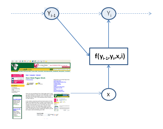
where $Z(\bar{x},y^{\prime})=\exp\sum_{j}\theta_{j}\phi_{j}(\bar{x},y^{\prime})$. The weight parameters $\theta$ of the factors are typically learned using discriminative learning methods for the target variable $y$ as an alternative to the probabilistic likelihood estimation method for computational efficiency reasons. There are two types of feature functions in representing a sequence [11]: (1) edge functions between two labels and (2) observation functions relating $x$ and $y$. Generally, $f_{j}(y_{t-1},y_{t},\bar{x},t)$ represents a feature function combining both edge and observation functions (Fig. 1). The following are examples of both types of feature functions in the handwriting recognition domain:

$$\phi_{j}(y_{i-1},y_{i})=\left\{\begin{array}[]{cc}1&if\,\,y_{i}="i"\,\,and\\ &y_{i-1}="n"\\ 0&otherwise\end{array}\right.$$

$$\phi_{j}(y_{i},x_{i})=\left\{\begin{array}[]{cc}1&if\,\,pixel(x_{i})=1\,\,and\\ &y_{i}="i"\\ 0&otherwise\end{array}\right.$$

The number of possible feature functions can be large but can be practically restricted to those found in the training set.

Generalizing to “global” factors over the entire sequence of observations where $F_{j}(\bar{x},\bar{y})=\sum_{t}^{n}f_{j}(y_{t-1},y_{t},\bar{x},t)$ and where $t$ is the position in the sequence of length $n$, the probability of the sequence $\bar{y}$ is then:

$$P(\bar{y}|\bar{x},\bar{\theta})=\frac{1}{Z(\bar{x},\bar{\theta})}\exp(\sum_{j}\theta_{j}F_{j}(\bar{x},\bar{y}))$$ (4)

where $Z(\bar{x},\bar{\theta})=\sum_{\bar{y}\in nP_{Y}}\exp(\sum_{j}\theta_{j}F_{j}(\bar{x},\bar{y})).$ The normalization constant $Z$ is computationally intractable [11] but does not need to be computed when predicting the labels in the sequence given the weights of the feature functions or when evaluating a sequence against one model.

Figure 1: CRF feature function relating observations and labels.

IV Methodology

We address the problem of sequence learning with a potentially infinite set of labels by learning several models. As in [3], we use the energy output of the output nodes, $E(x,y)$, before squashing by the softmax function, as the score of the factors in the CRF. We leverage from the neural network to discover non-linear feature functions in the case of the multi-layer perceptrons (MLPs) and we compare and contrast different neural network architectures. The Viterbi algorithm [7, 5] guides the step-by-step predictions to maximize the choice of each label $y$ with respect to the entire sequence. $P(\bar{y}|\bar{x},\bar{\theta})$ is then defined as follows:

$$P(\bar{y}|\bar{x},\bar{\theta})=\frac{\arg\max_{t_{1}...t_{n}}\prod_{t=1}^{n}P(y_{t}|y_{t-1},\bar{x}_{t},\bar{\theta})}{Z(\bar{x},\bar{\theta})}$$ (5)

Algorithm 1 describes the Viterbi evaluation of a sequence of observations $\bar{x}$ delimited by START and STOP tags combined with an approximate probabilistic evaluation of the entire sequence given the model. $P(\bar{y}|\bar{x},\bar{\theta})$ can be approximated using a partition function, $Z(\bar{x},\bar{\theta})$, that includes the maximum scores from the preceding step at each time step rather than the sum of scores of all possible sequences.

input: model, $\bar{x}$ //neural net and observation sequence

output: $\bar{y}$, $P(\bar{y}|\bar{x},\bar{\theta})$ //label sequence and probability

viterbi_crfs (model,$\bar{x}$)=

t $\leftarrow$ 0

$\alpha$[t]$\leftarrow$ initialize ($y_{0},x_{0})$

while t < length ($\bar{x}$)

t $\leftarrow$t + 1

$\alpha$[t] $\leftarrow$ forward ($\bar{x}_{t}$, $\alpha[t-1]$)

end

$y_{t}\leftarrow\arg\max_{y}\alpha[t]$

$\bar{y}$ $\leftarrow$ backtrack ($y_{t}$,$\alpha$)

score $\leftarrow$ $\max\alpha[t]$

$P(\bar{y}|\bar{x},\bar{\theta})$ $\approx$ $\frac{exp(score)}{\sum_{y}\exp(\alpha_{y}[t])}$

return $\bar{y}$, score, $P(\bar{y}|\bar{x},\bar{\theta})$

Algorithm 1 Viterbi algorithm for CRFs where forward and backtrack are functions as in the Viterbi algorithm and where alphas contains the information of all the possible outputs $y_{t}$ at each step $t$.

We compare and contrast the architectures of different neuroCRFs using the same methodology:

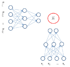
1. Combination of two multilayer perceptrons (CRF-MLP) trained with backpropagation where one MLP learns the weights of the transition factors between labels and another MLP learns the weights of the observation factors.

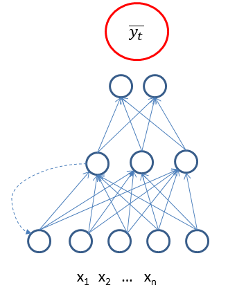
2. Recurrent neural network [12] (CRF-RNN) trained with backpropagation where the activations of the hidden units at the previous time step are added to the inputs at the next time step in the sequence.

3. Structured perceptron [5] (CRF-PRCPT) as described above II.

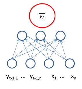
The different architectures compared are illustrated in Figs. 2, 3, and 4. Algorithm 2 describes the forward function of the Viterbi algorithm to compute $P(\bar{y}|\bar{x},\bar{\theta})$ in log space for CRF-MLP.

Figure 2: CRF-MLP - two MLPs combine to predict $y_{t}$

Figure 3: CRF-RNN - Elman network architecture where hidden node activations from the previous time step are added to the current input

Figure 4: CRF-PRCPT - Perceptron architecture including predictions from the previous time step

input: model, $\bar{x}$, $\alpha[t-1]$

//model, observations at time $t$, and $\alpha[]$

//model consists of one MLP for observations, $MLP_{obs},$
//and one MLP for edges, $MLP_{edges}$.

//$\alpha[t-1]$ is a list of tuples {$to,from,score\}$maximizing

//the score for each $to$ label at the previous step $t-1$

output: $\alpha[t]$

forward (model,$\bar{x}$, $\alpha[t-1]$)=

$obspreds$ $\leftarrow$ predict ($\bar{x}$, $MLP_{obs}$)

$edgepreds$ $\leftarrow$Ø

$\alpha[t]\leftarrow\textrm{\O}$

foreach $label\in Y_{model}$, the set of labels for the model

$edgepreds$ $\leftarrow$$edgepreds$ $\cup$ {predict ($label$, $MLP_{edges}$)}

foreach $label\in Y_{model}$

$to^{\prime},score^{\prime}$ $\leftarrow$

$arg\max_{\alpha[t-1]}(score+edgepreds[to]_{label}+obspreds_{label})$

$\alpha[t]\leftarrow\alpha[t]\cup\{label,to^{\prime},score^{\prime}\}$

return $\alpha[t]$

Algorithm 2 Forward function of Viterbi algorithm for CRF-MLP

Using stochastic gradient descent (SGD), training occurred when the label, as optimized for the overall sequence by the Viterbi algorithm, was incorrect. In addition, the weight updates were modulated with weight elimination regularization [13] for the MLPs:

$$w_{ij}=w_{ij}-\eta x_{i}(\delta_{j}+2\lambda\frac{w_{ij}}{(1+w_{ij}^{2})^{2}})$$

where $w_{ij}$ is the weight on the connection between $node_{i}$ and $node_{j}$, $i$ and $j$ denoting different contiguous layers, $\eta$ is the learning rate, $x_{i}$ is the activation at $node_{i}$, $\delta_{j}$ is the gradient at $node_{j}$ as calculated by the backpropagation algorithm, and $\lambda$ is the regularization parameter.

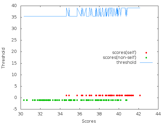
Our sequence classification metric is based on authentication biometrics using the false rejection rate (FRR) or false negatives and the false acceptance rate (FAR) or false positives leading to the identification of self vs. non-self. Several models are trained, each representing one type of sequence. Therefore, the conditional probability of a sequence given a model is not a calibrated probability because the training data is not assumed to represent the true distribution of all possible sequences and we do not know about other models (but we have examples of non-self). However, we can calibrate the score obtained evaluating sequences of self and non-self against the model with a threshold to report the equal error rate (EER), where the FRR equals the FAR, as follows. We map the scores obtained against testing examples of self to the positive class and scores obtained against testing examples of non-self to the negative class to obtain a linear model minimizing the sum of square errors separating the classes. We take the coefficient of regression for our threshold from which to compute the FRR and the FAR. Figure 5 illustrates how the threshold is determined from the scores of examples of self and non-self. We report results from the evaluation of this threshold on the validation set itself for a performance approximation. We report the r-square from the linear model to show the calibration of scores. The accuracy result is computed from the FRR and the FAR while the token accuracy is computed as the frequency of correct labels in the sequences. The F-score combines sequence classification accuracy and token accuracy results.

Figure 5: Threshold determination (coefficient of regression=37.25, r-square=0.31)

V Empirical Evaluation

The MLPs used a fixed learning rate set at 0.5 and a regularization parameter $\lambda$ set at 0.001. All neural nets used 1000 SGD examples or less if convergence to zero-error occurred during training. The weights for all neural nets were initialized to small values drawn from a normal distribution with zero mean and standard deviation 0.00015. The number of hidden nodes for the MLP-based architectures, CRF-MLP and CRF-RNN, was set to $\frac{n_{i}+n_{o}}{4}$ as in [14], where $n_{i}$ is the number of inputs and $n_{o}$ is the number of outputs. No attempt has been made to optimize the hyper-parameters of the different learners. The sigmoid function was the activation function for the nodes in the hidden layer and the derivative of the square loss function propagated the error at the output nodes.

The propagated loss in the structured perceptron was the difference between the predicted outcome and the actual outcome for each feature function relating inputs to outputs (0/1 loss). In addition, a mini-batch approach was used where the prediction error was averaged over 5 examples.

V-A OCR Dataset

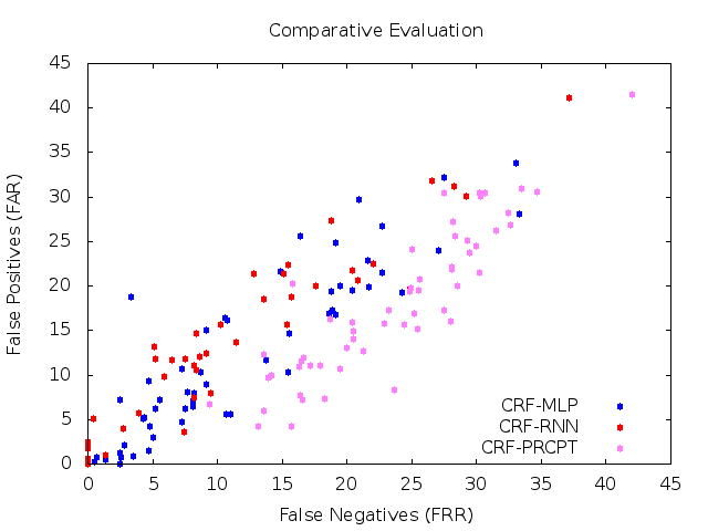
The OCR dataset [15] contains 52152 16x8 raster images of letters composing 55 distinct words of length ranging from 3 to 14. The number of examples per word varies from 71 to 151. Table I describes this dataset characteristics. A model is built for each word and tested against other words of the same length. At each iteration, the data for each word is randomly partitioned into 2/3 training and 1/3 testing to evaluate the FRR and compared against a random sample of ~100 exemplars of different letters of the same length to evaluate the FAR. Table II and Fig. 6 illustrates the results averaged over 5 iterations. While there is no significant statistical difference in the accuracy results between CRF-MLP and CRF-RNN, there is a significant statistical difference (two-sided p-value < 0.05) for the accuracy results between CRF-MLP and CRF-PRCPT and also between CRF-RNN and CRF-PRCPT. However, CRF-PRCPT has a greater token accuracy value at a significant statistical difference from both CRF-MLP and CRF-RNN. There is also a greater token accuracy value at a significant statistical different between CRF-MLP and CRF-RNN.

Word
Length	#words	#examples
3	9	1283
5	4	568
6	6	768
7	5	695
8	6	750
9	8	1047
10	5	584
11	3	304
12	2	298
13	3	313
14	3	266

Table I: OCR dataset characteristics

	Avg.	Avg.	Avg.	Avg.	Avg.	Avg.
Methods	FRR(%)	FAR(%)	Acc. (%)	$R^{2}$	Token Acc.(%)	F-score
CRF-MLP	11.81$\pm 13.08$	12.37$\pm 13.89$	87.90$\pm 08.84$	0.65$\pm 0.31$	93.03$\pm 04.36$	0.90$\pm 4.53$
CRF-RNN	8.95$\pm 14.04$	11.01$\pm 14.68$	90.02$\pm 10.18$	0.66$\pm 0.34$	85.17$\pm 07.70$	0.87$\pm 3.73$
CRF-PRCPT	23.59$\pm 09.63$	18.06$\pm 11.19$	79.17$\pm 07.38$	0.38$\pm 0.20$	95.44$\pm 02.96$	0.86$\pm 4.95$

Table II: Comparative results from neural-network based CRFs on the OCR dataset averaged over 5 iterations.

Figure 6: Comparative results from neural-network based CRFs on the OCR dataset. Each data point is the average results for one word over 5 iterations.

V-B Web Analytics

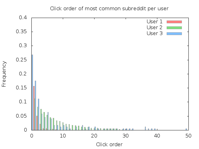
Another type of complex sequence can be found in our online activities. We extend previous work done in the context of Web browsing [9] to profile authentication from social media activities of Reddit users. Reddit is a public forum where anybody can create subreddits on any topics. We retrieved posts and comments using the Python Reddit API Wrapper (PRAW) from users associated to a seed user through at least one comment and from this pool of users selected at random 50 active users. There is a hard limit from Reddit to retrieve only the last 1000 posts and comments. The session pause delimiter (set to 30 minutes in Web browsing) was extended to one hour due to the sparsity of posts and/or comments. In contrast to Web browsing, the data of Reddit activities is sparse as evidenced by the large number of singleton sessions (Table III). Empirical analysis shows that the frequencies of the most common subreddits for a particular user follow the temporal order in which they were accessed (Fig. 7). As stated in [16], commonality is not a good discriminator. The entropy of the subreddits, as a measure of commonality, decreases according to their position in the session. To capture discriminating sequences, we modeled sessions of Reddit activities as n-gram sequences of length 4 and ignored shorter sequences. All users have sequences of various length up to length 6. Reddit user activities are modeled with CRFs as a sequence of posts/comments where the observations are the time-of-day, day-of-week, and subject header n-grams. A maximum of 100 most common n-grams per subreddit were extracted from the subject headers for computational efficiency. The labels are the subreddits of the posts/comments for a strongly supervised evaluation similar to the OCR dataset. Future work will evaluate the impact of a weakly-supervised approach with a subreddit concept hierarchy. Unlike the OCR dataset, the n-gram sequences are not i.i.d. Each user dataset was temporally partitioned into 90% training and 10% testing.

Figure 7: Frequencies of the most common subreddit by order visited for 3 users

sequence	Subreddit		#unique
Length	Entropy	#sessions	Subreddits
1	9.54	18580	1307
2	8.62	5305	703
3	7.90	2146	431
4	7.37	1155	293
5	6.80	655	194
6	6.49	428	155
>6	-	1231	372

Table III: Reddit dataset sequence length characteristics for 50 users.

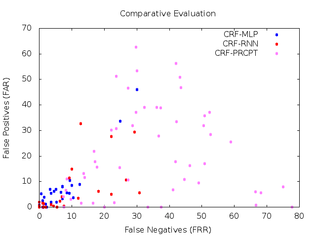
Table IV and Fig. 8 illustrates the results. There is a significant statistical difference (two-sided p-value < 0.05) in accuracy between the MLP-based architectures, CRF-MLP and CRF-RNN, and CRF-PRCPT but no statistical difference in accuracy between CRF-MLP and CRF-RNN. In addition, there is no statistical difference in token accuracy between CRF-RNN and CRF-PRCPT. We note that the correlation between labels is not as stable as in the OCR dataset which explains why CRF-MLP with an edge prediction network has lower token accuracy in this dataset.

	Avg.	Avg.	Avg.	Avg.	Avg.	Avg.
Methods	FRR(%)	FAR(%)	Acc. (%)	$R^{2}$	Token Acc.(%)	F-score
CRF-MLP	3.61$\pm 10.35$	3.83$\pm 11.37$	96.27$\pm 6.99$	0.87$\pm 0.25$	46.89$\pm 20.05$	0.61$\pm 0.11$
CRF-RNN	4.77$\pm 10.90$	3.21$\pm 09.34$	96.00$\pm 7.32$	0.81$\pm 0.26$	60.99$\pm 19.02$	0.72$\pm 0.12$
CRF-PRCPT	34.76$\pm 21.37$	21.37$\pm 21.35$	71.92$\pm 13.23$	0.23$\pm 0.25$	64.32$\pm 16.90$	0.66$\pm 0.11$

Table IV: Comparative results from neural-network based CRFs on the Reddit dataset

Figure 8: Comparative results from neural-network based CRFs on the Reddit dataset. Each data point is the average results for one individual over 5 iterations.

VI Conclusion

In summary, we have argued that the discriminative capabilities of CRFs in the structured prediction task do not necessarily carry over to the sequence classification task. Toward that end, we have compared and contrasted different architectures of neuroCRFs in two different tasks, the OCR hand-writing recognition task and the Web analytics task, with the same methodology. We have shown that CRFs, as a structured prediction approach, can also be applied to sequence classification by training several models for different types of sequence with potentially different labels, and calibrating the scores of each model (before softmax squashing) with a threshold determined by a linear model. While the structured perceptron performs better overall at the structured prediction task, the discriminative power of MLP based architectures, CRF-MLP and CRF-RNN, carries over to the sequence classification task albeit with some degradation in the structured prediction task. We note that CRF-MLP does better than CRF-RNN in the structured prediction task of the OCR hand-writing recognition task where the label transitions are consistent and modeled with an edge prediction network. Future work will further bridge the gap between sequence labeling and sequence classification as well as evaluate the impact of a weakly-supervised approach for user authentication in Web analytics with neural CRFs.

References

- [1] B. Zadrozny and C. Elkan, “Transforming classifier scores into accurate multiclass probability estimates,” in Proceedings of the eighth ACM SIGKDD international conference on Knowledge discovery and data mining, pp. 694–699, ACM, 2002.
- [2] Z. Xing, J. Pei, and E. Keogh, “A brief survey on sequence classification,” ACM SIGKDD Explorations Newsletter, vol. 12, no. 1, pp. 40–48, 2010.
- [3] T. Do, T. Arti, et al., “Neural conditional random fields,” in International Conference on Artificial Intelligence and Statistics, pp. 177–184, 2010.
- [4] A. Graves, “Generating sequences with recurrent neural networks,” CoRR, vol. abs/1308.0850, 2013.
- [5] M. Collins, “Discriminative training methods for hidden markov models: Theory and experiments with perceptron algorithms,” in Proceedings of the ACL-02 conference on Empirical methods in natural language processing-Volume 10, pp. 1–8, Association for Computational Linguistics, 2002.
- [6] O. Yakhnenko, A. Silvescu, and V. Honavar, “Discriminatively trained markov model for sequence classification,” in Data Mining, Fifth IEEE International Conference on, pp. 8–pp, IEEE, 2005.
- [7] L. R. Rabiner, “A tutorial on hidden markov models and selected applications in speech recognition,” in Proceedings of the IEEE, pp. 257–286, 1989.
- [8] J. Lafferty, A. McCallum, and F. Pereira, “Conditional random fields: Probabilistic models for segmenting and labeling sequence data,” in International Conference on Machine Learning ICML, 2001.
- [9] M. Abramson, “Learning temporal user profiles of web browsing behavior,” in 6th ASE International Conference on Social Computing SocialCom, (Stanford, CA), May 2014.
- [10] K. P. Murphy, Machine learning: a probabilistic perspective. The MIT Press, 2012.
- [11] C. Sutton and A. McCallum, “An introduction to conditional random fields,” arXiv preprint arXiv:1011.4088, 2010.
- [12] J. L. Elman, “Finding structure in time,” Cognitive science, vol. 14, no. 2, pp. 179–211, 1990.
- [13] Y. S. Abu-Mostafa, M. Magdon-Ismail, and H.-T. Lin, Learning from data. AMLBook, 2012.
- [14] J. Goecks and J. Shavlik, “Learning users’ interests by unobtrusively observing their normal behavior,” in Proceedings of the 5th international conference on Intelligent user interfaces, pp. 129–132, ACM, 2000.
- [15] R. H. Kassel, A comparison of approaches to on-line handwritten character recognition. PhD thesis, Massachusetts Institute of Technology, 1995.
- [16] E. Shi, Y. Niu, M. Jakobsson, and R. Chow, “Implicit authentication through learning user behavior,” in Information Security, pp. 99–113, Springer, 2011.