A Hydrodynamic Approach to the Study of Anisotropic Instabilities in Dissipative Relativistic Plasmas

Abstract

We develop a purely hydrodynamic formalism to describe collisional, anisotropic instabilities in a relativistic plasma, that are usually described with kinetic theory tools. Our main motivation is the fact that coarse-grained models of high particle number systems give more clear and comprehensive physical descriptions of those systems than purely kinetic approaches, and can be more easily tested experimentally as well as numerically. Also they make it easier to follow perturbations from linear to non-linear regimes. In particular, we aim at developing a theory that describes both a background non-equilibrium fluid configurations and its perturbations, to be able to account for the backreaction of the latter on the former. Our system of equations includes the usual conservation laws for the energy-momentum tensor and for the electric current, and the equations for two new tensors that encode the information about dissipation. To make contact with kinetic theory, we write the different tensors as the moments of a non-equilibrium one-particle distribution function (1pdf) which, for illustrative purposes, we take in the form of a Grad-like ansatz. Although this choice limits the applicability of the formalism to states not far from equilibrium, it retains the main features of the underlying kinetic theory. We assume the validity of the Vlasov-Boltzmann equation, with a collision integral given by the Anderson-Witting prescription, which is more suitable for highly relativistic systems than Marle’s (or Bhatnagar, Gross and Krook) form, and derive the conservation laws by taking its corresponding moments. We apply our developments to study the emergence of instabilities in an anisotropic, but axially symmetric background. For small departures of isotropy we find the dispersion relation for normal modes, which admit unstable solutions for a wide range of values of the parameter space.

I Introduction

The study of plasma instabilities is of major importance in a wide range of areas as e.g. astrophysics, cosmology, Tokamaks, lasers, etc. In the non-relativistic regime, there is a well established hydrodynamic formalism, magnetohydrodynamics (MHD), that consists of the Navier-Stokes equation for the momentum, the continuity equation for the mass density and the Maxwell equations for the electromagnetic fields, complemented with a corresponding Ohm’s law. This theory is known as a first order theory, as it is the result of a first order expansion in gradients of the distribution function around equilibrium. When turning to relativistic domains, it is possible to extend to it the tools employed to study ideal fluids, i.e. the Euler equation. But when dissipative processes are taken into account, the natural generalization of Navier-Stokes equation to relativistic velocities proved to fail, as the solutions are all unstable and non-causal HisLin83 . Among the relativistic first order theories, the Eckart Eck40 and Landau-Lifshitz LL6 formulations are the best known.

Since the seventies several theories were proposed to overcome these drawbacks, among them the so-called second order theories (among several possible strategies sps ), as e.g. the ones developed by Israel and Stewart SOTs . Both formalisms, first and second order, are based on a gradient expansion of the 1pdf around equilibrium, and in this sense their applicability is limited to small deviations from local equilibrium. There is another set of theories, not anchored to a kinetic equation, and that are not the result of a perturbative expansion, they are known as Divergence Type Theories (DTT) and were developed by Liu and others liu72 ; LiuMuRu86 ; GeLin91 . They are exact and thus can describe systems well away from equilibrium, but their drawback is that they are not clearly linked to microscopic physics.

A paradigmatic case of relativistic plasma is the nuclear matter created in the experiments ongoing at the Relativistic Heavy-Ion Collider (RHIC) at Brookhaven National Laboratory and at the Large Hadron Collider (LHC) at CERN. There are clear experimental signatures that the relativistic matter created in the collisions, a quark-gluon plasma, behaves as a strongly coupled system. Consequently RHIC’s plasmas offer a unique scenario to test relativistic hydrodynamics. Indeed pure hydrodynamic models proved to be very successful in describing the main features of these plasmas, thus strongly improving the understanding of those systems. For a comprehensive review on relativistic hydrodynamics and RHIC’s plasmas see Ref. citeSch14,JeHe15,Rom16 and references therein.

RHIC’s plasmas show two special features: high degree of anisotropy and quick thermalization. In fact, the longitudinal expansion of the fireball causes the system to be much colder in the longitudinal direction than in the transverse ones. Such an out of equilibrium state favors the presence of instabilities and cannot be studied with the usual hydrodynamic models based on perturbative schemes around equilibrium configurations. Although the development of an anisotropic hydrodynamics Str14b ; TRFS15 is a very important step toward the understanding of those systems, it is not clear if the resulting hydrodynamics retains enough features of the underlying kinetic regime to provide a satisfactory description of instabilities. Concerning hydrodinamization, it is believed that the instabilities favored by the anisotropic background contribute to such a process. Indeed, Mrówczyńzky showed that they play a substantial rôle in the dynamics of the early stages of the evolution of quark-gluon plasmas. For more details on this issue, see Ref. MSS16 and references therein.

There are experimental evidences of the presence of magnetic fields in the RHIC’s plasmas Hua16 . Most of the above mentioned anisotropic hydrodynamic models do not take into account electromagnetic fields and consequently are not suitable to give a realistic explanation of the observations.

The main purpose of our study is to start building a consistent magnetohydrodynamic theory to describe strongly coupled, high energy plasmas, without having to address to kinetic theory for each different system under study, and that includes both the background and its perturbations in a consistent way.

To facilitate the calculations we consider a massless Abelian plasma. Although a non-Abelian theory is needed to correctly describe the plasmas created at RHICs, our choice has the advantage of simplifying the mathematics without depriving the model of physical relevance MaMr06 ; PRC12a ; PRC09 ; PRC10b ; MSS16 .

To give our model a kinetic theory support, we write the different tensors as momenta of a distribution function and to obtain their evolution equations we invoke a mean field kinetic model described by the Boltzmann-Vlasov equation. As for the collision integral, most of the literature uses the BGK (Bhatnagar, Gross and Krook) relaxation time model, as it allows to effectively handle distributions other than the Maxwell-Boltzmann. Its relativistic generalization was developed by Marle and is of the form $C(f)=-m(f-f_{0})/\tau$ marle1 ; marle2 . In the classical limit, Marle’s formulation gives the same result for the transport coefficients as the classical BGK model. However, in the extreme relativistic limit the results for the transport coefficients with Marle’s formulation differ functionally from the ones calculated with the relativistic Grad moment method. Anderson and Witting and-witt1 ; and-witt2 ; TI10 proposed an improvement of Marle’s collision integral of the form $C(f)=-u_{\mu}p^{\mu}(f-f_{0})/\tau$ with $u_{\mu}$ the four velocity of the gas. In the classical limit this expression gives the same classical results as Marle’s, since in that limit $u_{\mu}p^{\mu}\rightarrow m$, and in the extreme relativistic limit it produces the same transport coefficients that are obtained via the relativistic Grad moment method. Consequently, as we are dealing with a highly relativistic system we shall adopt the Anderson-Witting prescription instead of the BGK collision kernel in Marle’s form, generally adopted in the literature.

We consider a model where the distribution function is the product of an equilibrium expression times a non-equilibrium part. The former is isotropic and homogeneous in the momenta, and also depends on a thermal potential that accounts for possible excess of particles over antiparticles. We specify it by demanding that the ideal energy-momentum tensor $T^{\mu\nu}$ calculated from it, corresponds to the Landau-Lifshitz prescription, whereby in the rest frame $T^{0i}=0$ LL6 . The latter contains all the information about anisotropies and dissipation. For the collision integral, we only demand it to be linear in the tensors that describe non-equilibrium features, i.e., ohmic and viscous dissipation, and possible anisotropies in the momenta distribution. The main motivation behind this choice is to avoid mathematical complexity.

Our model is not truly reliable for arbitrarily large anisotropy, as it will be discussed below (see also Ref. MAEC17 ). Within its range of validity, however, it fully captures nonlinearities coming from the convective derivative terms and from direct coupling of the hydrodynamic variables to the electromagnetic fields in the equations of motion. These are the only nonlinearities in the usual magnetohydrodynamics, where dissipative terms are assumed to be linear. For this reason, we believe the hydrodynamic equations to be introduced below (eqs. (42) to (47)) are a valid generalization of MHD to the relativistic regime. Moreover, we also believe any consistent relativistic dynamics of real fluids will converge to this formalism within its range of validity.

We build our formalism by writing the different tensors as moments of the distribution function, and find their evolution equations by taking the corresponding moments of the Vlasov-Boltzmann equation. By projecting those equations along the four velocity and onto its orthogonal hypersurface we obtain five hydrodynamic equations: for the charge density, for the energy density, for the velocity field and for the two tensors that describe dissipation. Together with Maxwell equations they form our magnetohydrodynamic model.

As an application of our formalism we study the transverse instabilities that appear in fluctuations around an anisotropic background. These were first discussed by E. S. Weibel weibel59 in a non-relativistic setting, and then in the relativistic regime in Refs. sschl04 ; ach1 ; ach2 among others. In the non-relativistic theory a purely macroscopic approach already exists, see e.g. Refs. basu02 ; brdeu06 ; bret06 . Our aim is to generalize these macroscopic approaches to relativistic theories, accounting for dissipative effects. Of course the Weibel instability is not the only possible instability of relativistic plasmas, see Ref. bret09 for a detailed analysis of the different kinds of instabilities in Abelian plasmas. Moreover when considering non-Abelian plasmas new kinds of instabilities appear, as can be seen in e.g. Ref. mama07 . In order to avoid a heavy mathematical content, we leave for forthcoming manuscripts the analysis of the other instabilities in Abelian plasmas, as well as the extension of our formalism to the non-Abelian case.

The manuscript is organized as follows, in Section II we build the 1pdf. In Section III we build the magnetohydrodynamic formalism, by deducing the tensors and the equations they must satisfy. In Section IV we linearize the previously found equations around a background with anisotropic pressure, and find the dispersion relation for the normal modes, consistent with the limitations of the model. For a wide range of values of the parameter space, our model predicts the excitation of instabilities, whose features are in agreement with results previously found in the literature. To illustrate those the dependence on the different parameters of the model, we plot this relation for several values of them. Finally, in Section V we summarize our conclusions and comment on future perspectives. We work with natural units, i.e., $c=\hbar=k_{B}=1$ and with signature $\left(-,+,+,+\right)$.

II Kinetic Theory

In this section we shortly review some basics of kinetic theory of plasmas and build the 1pdf of our model. In the mean field approach the kinetic equation for a plasma with electromagnetic fields is the Boltzmann-Vlasov equation, which reads

$$p^{\mu}\left[\frac{\partial}{\partial x^{\mu}}-eF_{\mu\rho}\frac{\partial}{\partial p_{\rho}}\right]f\left(x^{\mu},p^{\mu}\right)=I_{col}\left(x^{\mu},p^{\mu}\right)$$ (1)

where $f\left(x^{\mu},p^{\mu}\right)$ is the distribution function, $I_{col}\left(x^{\mu},p^{\mu}\right)$ the collision integral (to be defined below). Integration over momentum is done with the invariant volume element

$$Dp=\frac{2d^{4}p}{\left(2\pi\right)^{3}}\delta\left(p^{2}\right)=\frac{d^{4}p}{\left(2\pi\right)^{3}p}\left[\delta\left(p^{0}-p\right)+\delta\left(p^{0}+p\right)\right]$$ (2)

As stated in the Introduction, we shall deal with the massless case, whereby $p^{2}=0$, with $p^{0}$ having either sign: positive for positively charged particles, and negative for negatively charged antiparticles.

The current and the matter energy momentum tensor (EMT for short) are defined as usual, namely

$$J^{\mu}=e\int Dp\;p^{\mu}f$$ (3)

and

$$T^{\mu\nu}=\int Dp\;p^{\mu}p^{\nu}f$$ (4)

$F_{\mu\nu}$ in eq. (1) is the Maxwell tensor $F_{\mu\nu}=\partial_{\mu}A_{\nu}-\partial_{\nu}A_{\mu}$, with $A^{\mu}$ the electromagnetic four potential. Inclusion of the Maxwell field as an independent degree of freedom is of course the main goal of this analysis. The Maxwell field obeys Maxwell’s equations sourced by the current $J^{\mu}$ defined in eq. (3)

$$F_{\mu\nu,\rho}+F_{\nu\rho,\mu}+F_{\rho\mu,\nu} = 0$$

$$F^{\mu\nu}_{,\nu} = 4\pi J^{\mu}$$ (5)

Antisymmetry of $F_{\mu\nu}$ demands charge conservation

$$J^{\mu}_{,\mu}=0$$ (6)

Associated to the Maxwell field there is an electromagnetic energy momentum tensor $T_{EM}^{\mu\nu}$ [MTW ]

$$T_{EM}^{\mu\nu}=\frac{1}{4\pi}\left\{F^{\mu\rho}F^{\nu}_{\;\rho}-\frac{1}{4}\eta^{\mu\nu}F^{\rho\sigma}F_{\rho\sigma}\right\}$$ (7)

$\eta^{\mu\nu}$ is Minkowsky metric. The full energy momentum tensor $T_{F}^{\mu\nu}=T^{\mu\nu}+T_{EM}^{\mu\nu}$ is conserved: $T^{\mu\nu}_{F,\nu}=0$. We may also use Maxwell’s equations to compute $T^{\mu\nu}_{EM,\nu}=-F^{\mu\rho}J_{\rho}$ and thus rewrite the conservation law as

$$T^{\mu\nu}_{,\mu}=F^{\nu\mu}J_{\mu}$$ (8)

The conservation laws (6) and (8) may be obtained from the zeroth and first momenta of the Boltzmann equation, provided that

$$\int Dp\;I_{col}=\int Dp\;p^{\nu}I_{col}=0$$ (9)

We consider a classical (i.e., not quantum) system. Then in an equilibrium state the distribution function takes the form

$$f_{eq}=e^{\mathrm{sign}\left[p^{0}\right]\left(\alpha+\beta_{\mu}p^{\mu}\right)}$$ (10)

and the collision integral vanishes. In the previous expression $\beta_{\mu}=\beta u_{\mu}$, $\beta=1/T$, where $T$ is the temperature. Following Israel [SOTs ], we call $\alpha$ the thermal potential; $\mu=T\alpha$ is the chemical potential that accounts for the excess of particles over antiparticles. We choose to identify the velocity $u^{\mu}$ and energy density $\rho$ as the timelike eigenvector of $T^{\mu\nu}$ and its eigenvalue, i.e., $T^{\mu\nu}_{id}u_{\nu}=-\rho u^{\mu}$, i.e., we work in the Landau-Lifshitz frame LL6 . Also we define the charge density as $\rho_{q}=-u_{\mu}J^{\mu}$. In this case the ideal part of the current and EMT take the form

$$J^{\mu}_{id}=\rho_{q}u^{\mu}$$ (11)

and

$$T^{\mu\nu}_{id}=\rho\left[u^{\mu}u^{\nu}+\frac{1}{3}h^{\mu\nu}\right]$$ (12)

where the fluid four velocity is normalized as $u^{2}=-1$ and $h^{\mu\nu}=\eta^{\mu\nu}+u^{\mu}u^{\nu}$ is the projector onto hypersurfaces orthogonal to $u^{\mu}$. After evaluating the current and the EMT we read

$$\rho_{q}=\frac{2eT^{3}}{\pi^{2}}\sinh\alpha$$ (13)

and

$$\rho=\frac{6T^{4}}{\pi^{2}}\cosh\alpha$$ (14)

Eq. (13) shows that when $\alpha=0$, the number of particles equals the number of antiparticles and consequently the net charge of the plasma is zero. Moreover expr. (13) and (14) show that the temperature $T$ and thermal potential $\alpha$ are univocally determined by the charge and energy densities.

Observe that we may also introduce electric and magnetic fields relative to the fluid rest frame by writing

$$F^{\mu\nu}=u^{\mu}E^{\nu}-E^{\mu}u^{\nu}+\epsilon^{\mu\nu\rho\sigma}B_{\rho}u_{\sigma}$$ (15)

Thus in the rest frame $E^{a}=F^{0a}$ and $B_{a}=\left(1/2\right)\epsilon_{abc}F^{bc}$.

To describe non-equilibrium states, we choose to parametrize the distribution function in the form:

$$f=f_{eq}\left[1+Z\right]$$ (16)

We demand that $Z$ satisfies the constraints

$$\int Dp\;f_{eq}\;u_{\mu}p^{\mu}Z=\int Dp\;f_{eq}\;u_{\mu}p^{\mu}p^{\nu}Z=0$$ (17)

which implies that the ideal forms (11) and (12), with (13) and (14), are preserved. Note that in expression (16), $Z$ is not small in front of $1$. We define the entropy flux in the usual way, i.e.,

$$S^{\mu}=-\int Dp\;\mathrm{sign}\left[p^{0}\right]p^{\mu}f\left[\ln f-1\right]$$ (18)

which satisfies the equation

$$S^{\mu}_{,\mu}=-\int Dp\;\mathrm{sign}\left[p^{0}\right]\;I_{col}\ln f$$ (19)

showing that there is no entropy production from an equilibrium state. To enforce positiveness of expression (19), we must choose an appropriate collision integral. In this manuscript we concentrate in writing down a simplest possible dissipative relativistic magnetohydrodynamic formalism to describe high energy plasma features (specially its instabilities) without having to resource to kinetic theory for each specific problem. The straightforward way to do this is to linearize expr. (19) to first order in $Z$, i.e., to write

$$S^{\mu}_{,\mu}=-\int Dp\;\mathrm{sign}\left[p^{0}\right]Z\;I_{col}$$ (20)

This expression suggests to consider a collision integral of the Anderson-Witting form and-witt1 ; and-witt2 ; TI10 , namely

$$I_{col}=\frac{u_{\rho}p^{\rho}}{\tau}f_{eq}Z$$ (21)

with $\tau$ a relaxation time. This form of $I_{col}$ guarantees that the $H$ theorem is satisfied, namely:

$$S^{\mu}_{,\mu}=\int Dp\;\frac{\left|u_{\rho}p^{\rho}\right|}{\tau}f_{eq}Z^{2}\geq 0$$ (22)

as well as constraints (9). To account to dissipative processes in the dynamics we split the electric current and the EMT as

$$J^{\mu}=\rho_{q}u^{\mu}+j^{\mu}$$ (23)

and

$$T^{\mu\nu}=\rho\left[u^{\mu}u^{\nu}+\frac{1}{3}h^{\mu\nu}\right]+\Pi^{\mu\nu}$$ (24)

where

$$j^{\mu}=e\int Dp~{}p^{\mu}f_{eq}Z$$ (25)

and

$$\Pi^{\mu\nu}=\int Dp~{}p^{\mu}p^{\nu}f_{eq}Z$$ (26)

describe dissipative effects.

At this point it is necessary to provide an explicit form for $Z$, such that the dissipative parts of the current and EMT may be computed. Since the EMT is traceless, both conserved currents amount to $13$ degrees of freedom, of which $\alpha$, $T$ and $u^{\mu}$ account for $5$. It is natural to assume that $Z$ depends on $8$ additional parameters, to which we must add $5$ more to have enough freedom to enforce the constraints (17). We arrive at the right number if $Z$ depends on a new vector field $Z^{\mu}$ and a tensor field $Z^{\mu\nu}$ such that $u_{\mu}u_{\nu}Z^{\mu\nu}=0$. We further split them in longitudinal and transverse components along $u^{\mu}$: $Z^{\mu}=e\zeta^{\mu}+au^{\mu}$ and $Z^{\mu\nu}=\zeta^{\mu\nu}+b^{\mu}u^{\nu}+u^{\mu}b^{\nu}$. The simplest Lorentz invariant form for $Z$ is the linear one

$$Z=\frac{\tau}{2\left|u_{\rho}p^{\rho}\right|}\left[e\zeta_{\rho}p^{\rho}+\zeta_{\rho\sigma}p^{\rho}p^{\sigma}+au_{\rho}p^{\rho}+\frac{1}{2}\left(b_{\rho}u_{\sigma}+u_{\rho}b_{\sigma}\right)p^{\rho}p^{\sigma}\right]$$ (27)

hence $S^{\mu}_{;\mu}\geq 0$. Since $p^{\mu}$ is restricted to the null cone, we may impose one further condition on $\zeta^{\mu\nu}$: we chose it to be traceless. The functional form (27) can also be obtained by using a variational method to impose constraints that describe the non-equilibrium state of the system, such as the Entropy Production Variational Method epvm-rev ; christen14 ; christen ; christen2 . It can be proved that in out-of-equilibrium linear thermodynamics, stationary states are extrema of the entropy production rate. Moreover, at linear order in the entropy production, the results are equivalent to those obtained through the Grad approach PRC10a ; PRC12a ; PRC13a ; epv-2 .

Recalling that $\zeta_{\rho}$ and $\zeta_{\rho\sigma}$ are transverse and the latter is traceless, constraints (17) read

$$0 = \cosh\alpha\;a+3T\sinh\alpha\;b_{\rho}u^{\rho}$$

$$0 = \sinh\alpha\left[-\frac{e}{3}\zeta^{\nu}+au^{\nu}\right]+4T\cosh\alpha\;b_{\rho}\left(u^{\nu}u^{\rho}+\frac{1}{3}h^{\nu\rho}\right)$$ (28)

whose solutions are

$$a = b_{\rho}u^{\rho}=0$$ (29)

$$b^{\nu} = \frac{e}{4T}\tanh\alpha\;\zeta^{\nu}$$ (30)

Replacing in eq. (27) we finally obtain

$$Z=\frac{\tau}{2\left|u_{\rho}p^{\rho}\right|}\left[e\zeta_{\rho}p^{\rho}+\zeta_{\rho\sigma}p^{\rho}p^{\sigma}+\frac{e}{4T}\tanh\alpha\;\zeta_{\rho}u_{\sigma}p^{\rho}p^{\sigma}\right]$$ (31)

The tensors $\zeta^{\mu}$ and $\zeta^{\mu\nu}$ are the new ones mentioned in the Introduction. They account for the different dissipative processes: the former represents conduction currents, while the latter is associated to viscous stresses.

III Building the Hydrodynamics

The different tensors that describe our hydrodynamical model are written in terms of the distribution function in the usual way, namely

$$A^{\mu_{1},\ldots\mu_{n}}_{s}=\int Dp\;\left(\mathrm{sign}\left[p^{0}\right]\right)^{s}p^{\mu_{1}}\ldots p^{\mu_{n}}f$$ (32)

with $s=0$ or $1$. The conservation laws obeyed by these tensors are obtained by taking the corresponding moments of eq. (1), their general form then being

$$A^{\mu\mu_{1},\ldots\mu_{n}}_{s,\mu}-e\sum_{i=1}^{n}F^{\mu_{i}}_{\;\mu}A^{\mu\mu_{1},\ldots\left(\mu_{i}\right)\ldots\mu_{n}}_{s}=-I_{s}^{\mu_{1},\ldots\mu_{n}}$$ (33)

where the notation $A^{\mu\mu_{1},\ldots\left(\mu_{i}\right)\ldots\mu_{n}}_{A}$ means that $\mu_{i}$ is excluded, and

$$I_{s}^{\mu_{1},\ldots\mu_{n}}=-\int Dp\;\left(\mathrm{sign}\left[p^{0}\right]\right)^{s}p^{\mu_{1}}\ldots p^{\mu_{n}}I_{col}$$ (34)

Each momentum may be written as $A^{\mu_{1},\ldots\mu_{n}}_{s}=A^{\mu_{1},\ldots\mu_{n}}_{s,ideal}+A^{\mu_{1},\ldots\mu_{n}}_{s,dis}$ with $A^{\mu_{1},\ldots\mu_{n}}_{s,ideal}$, $A^{\mu_{1},\ldots\mu_{n}}_{s,dis}$ and $I_{s}^{\mu_{1},\ldots\mu_{n}}$ totally symmetric and traceless on any two indices.

From expr. (32) we thus obtain the different tensors of our model; in particular, the current previously introduced in eq. (23) is $J^{\mu}=eA^{\mu}_{0}$ and the EMT defined in eq. (24) is $T^{\mu\nu}=A^{\mu\nu}_{0}$. As discussed above, our theory has $13$ non trivial degrees of freedom $\alpha$, $T$, $u^{\mu}$, $\zeta^{\mu}$ and $\zeta^{\mu\nu}$. The charge and EMT conservation laws provide $5$ equations. To obtain the necessary $8$ supplementary equations we will consider two more tensors $A^{\mu\nu}_{1}$ and $A^{\mu\nu\rho}_{1}$. The equations we seek are $h_{\mu\lambda}\left[A^{\nu\lambda}_{1,\nu}+I^{\lambda}_{1}\right]=0$ and $\left(h_{\mu\lambda}h_{\nu\sigma}-\left(1/3\right)h_{\mu\nu}h_{\lambda\sigma}\right)\left[A^{\rho\lambda\sigma}_{1,\rho}+I^{\lambda\sigma}_{1}\right]=0$. The former provides $3$ new equations, and the latter the remaining $5$.

Let us now compute the relevant tensors. At first level:

$$A^{\mu}_{0}=q_{1}T^{3}u^{\mu}+\Lambda e\tau T^{3}\zeta^{\mu}$$ (35)

where $q_{1}=\left(2/\pi^{2}\right)\sinh\alpha$, $q_{2}=\left(2/\pi^{2}\right)\cosh\alpha$ and $\Lambda=\left(4q_{2}^{2}-3q_{1}^{2}\right)/24q_{2}$.

The vector $A^{\mu}_{1}$ is the particle number current, which in our model is likewise conserved. However, this is actually a drawback of the model, which is too simplistic to account for pair creation and annihilation. We therefore pass it over and consider other currents whose conservation laws may be expected to be less sensitive to those effects. In other words, while charge and EMT conservation hold for any form of the collision integral, as long as the constraints eq. (9) are enforced, the conservation laws we are writing down for the other tensors depend on the precise form of the collision integral. In this sense, we may regard the Anderson - Witting (AW) collision integral as a first order approximation in a series expansion in which progressively more complex interactions are taken into account. The particle number current is highly sensitive to the higher order terms in this expansion, because in this case the production term computed from the AW collision integral vanishes; therefore the first order equation is not reliable. For $A^{\mu\nu}_{1}$ and $A^{\mu\nu\rho}_{1}$, as we shall see presently, the AW collision integral gives nontrivial production terms, and so the dependence on further improvements of the collision integral may be expected to be weaker.

At second level:

$$A^{\mu\nu}_{0}=3q_{2}T^{4}\left[u^{\mu}u^{\nu}+\frac{1}{3}h^{\mu\nu}\right]+\frac{4q_{2}}{5}\tau T^{5}\zeta^{\mu\nu}$$ (36)

$$A^{\mu\nu}_{1}=3q_{1}T^{4}\left[u^{\mu}u^{\nu}+\frac{1}{3}h^{\mu\nu}\right]+\kappa_{1}e\tau T^{4}\left[\zeta^{\mu}u^{\nu}+\zeta^{\nu}u^{\mu}\right]+\eta_{1}\tau T^{5}\zeta^{\mu\nu}$$ (37)

with $\eta_{0}=4q_{2}/5$, $\eta_{1}=4q_{1}/5$ and $\kappa_{1}=\left(q_{2}^{2}-q_{1}^{2}\right)/{2q_{2}}$. Finally, at third level

$$A^{\mu\nu\rho}_{1} = 12q_{2}T^{5}\left[u^{\mu}u^{\nu}u^{\rho}+\frac{1}{3}\left(h^{\mu\nu}u^{\rho}+h^{\mu\rho}u^{\nu}+h^{\rho\nu}u^{\mu}\right)\right]$$ (38)

$$- \frac{q_{1}}{2}e\tau T^{5}\left[\zeta^{\mu}u^{\nu}u^{\rho}+\zeta^{\nu}u^{\mu}u^{\rho}+\zeta^{\rho}u^{\nu}u^{\mu}+\frac{1}{5}\left(h^{\mu\nu}\zeta^{\rho}+h^{\mu\rho}\zeta^{\nu}+h^{\rho\nu}\zeta^{\mu}\right)\right]$$

$$+ 4\tau q_{2}T^{6}\left(\zeta^{\mu\nu}u^{\rho}+\zeta^{\mu\rho}u^{\nu}+\zeta^{\rho\nu}u^{\mu}\right)$$

There remains to compute the momenta of the collision integral. To do that we observe that $I_{s}^{\mu_{1},\ldots\mu_{n}}=-\frac{1}{\tau}u_{\mu}A_{s,dis}^{\mu\mu_{1},\ldots\mu_{n}}$ and therefore

$$I_{0} = I_{1}=I_{0}^{\mu}=0$$ (39)

$$I_{1}^{\nu} = e\kappa_{1}T^{4}\zeta^{\nu}$$ (40)

$$I_{1}^{\nu\rho} = -\frac{q_{1}}{2}eT^{5}\left(\zeta^{\nu}u^{\rho}+\zeta^{\rho}u^{\nu}\right)+4q_{2}T^{6}\zeta^{\nu\rho}$$ (41)

Our hydrodynamic equations for $A_{0}^{\mu}$, $A_{0}^{\mu\nu}$, $A_{1}^{\mu\nu}$ and $A_{1}^{\mu\nu\rho}$ are extracted from the ones obtained from (33), by projecting them along $u^{\mu}$ and onto the surfaces defined by $h^{\mu\nu}$. We define the new variables $q_{0}=q_{1}T^{3}$, $L_{0}=\Lambda T^{3}$ and $\rho_{0}=3q_{2}T^{4}$. For $A^{\mu}_{0}$ we have only one equation, namely charge conservation eq. (6). In terms of hydrodynamic variables it reads

$$q^{\prime}_{0}+q_{0}u^{\mu}_{,\mu}+e\tau\left(L_{0,\mu}\zeta^{\mu}+L_{0}\zeta^{\mu}_{,\mu}\right)=0$$ (42)

where ${}^{\prime}\equiv u^{\mu}\partial_{\mu}$. The equations for $A^{\mu\nu}_{0}$ are the EMT conservation eqs. (8). Projected along $u^{\nu}$ it gives

$$-\rho^{\prime}_{0}-\frac{4}{3}\rho_{0}u^{\mu}_{,\mu}-\frac{1}{2}\tau\eta_{0}T^{5}\zeta^{\mu\nu}\sigma_{\mu\nu}=e^{2}\tau L_{0}F_{\nu\rho}u^{\nu}\zeta^{\rho}$$ (43)

where

$$\sigma^{\mu\nu}=h^{\mu\rho}h^{\nu\lambda}\left[u_{\rho,\lambda}+u_{\lambda,\rho}-\frac{2}{3}h_{\rho\lambda}u^{\sigma}_{,\sigma}\right]$$ (44)

is the shear tensor, and the projection orthogonal to $u^{\nu}$ yields

$$\frac{4}{3}\rho_{0}\left(u^{\nu}\right)^{\prime}+\frac{1}{3}h^{\mu\nu}\rho_{0,\mu}+\tau\left(\eta_{0}T^{5}\right)_{,\mu}\zeta^{\mu\nu}+\tau\eta_{0}T^{5}h^{\nu}_{\rho}\zeta^{\mu\rho}_{,\mu}=eh^{\mu\nu}F_{\mu\rho}\left(q_{0}u^{\rho}+e\tau L_{0}\zeta^{\rho}\right)$$ (45)

$A_{1}^{\mu\nu}$ and $A_{1}^{\mu\nu\rho}$ provide the necessary supplementary equations. For $A_{1}^{\mu\nu}$ we only need its spatial projection which, after a bit of algebra yields

$$0 = \left(q_{1}T^{4}\right)_{,\mu}h^{\mu\nu}+4q_{1}T^{4}\left(u^{\nu}\right)^{\prime}+e\tau\left(\kappa_{1}T^{4}\right)^{\prime}\zeta^{\nu}+e\kappa_{1}T^{4}\zeta^{\nu}$$ (46)

$$+ e\tau\kappa_{1}T^{4}h^{\nu}_{\sigma}\left(\zeta^{\sigma}\right)^{\prime}+e\tau\kappa_{1}T^{4}\zeta^{\nu}u^{\mu}_{,\mu}+\tau\left(\eta_{1}T^{5}\right)_{,\mu}\zeta^{\mu\nu}+\tau\eta_{1}T^{5}h^{\nu}_{\sigma}\zeta^{\mu\sigma}_{,\mu}$$

$$+ e\tau\kappa_{1}T^{4}u^{\nu}_{,\mu}\zeta^{\mu}-eq_{2}T^{3}F^{\nu}_{\;\mu}u^{\mu}-e^{2}\tau\Lambda_{1}T^{3}h^{\nu}_{\rho}F^{\rho}_{\;\mu}\zeta^{\mu}$$

If we only keep the last term in the first line and the term involving the electric field in the last line we see this is a generalized Ohm’s law.

Finally, the traceless, doubly transverse projection of the equation for $A_{1}^{\mu\nu\rho}$ reads

$$-4q_{2}T^{6}\zeta^{\alpha\beta} = 4q_{2}T^{5}h^{\rho\beta}h^{\alpha\nu}\left[u_{\nu,\rho}+u_{\rho,\nu}-\frac{2}{3}h_{\rho\nu}u^{\mu}_{,\mu}\right]$$ (47)

$$- \frac{e\tau}{10}\eta_{1,\mu}\left[h^{\mu\alpha}h^{\beta}_{\rho}\zeta^{\rho}+h^{\mu\beta}h^{\alpha}_{\nu}\zeta^{\nu}-\frac{2}{3}h^{\alpha\beta}\zeta^{\mu}\right]$$

$$- \frac{e\tau}{2}q_{1}T^{5}h^{\alpha}_{\nu}h^{\beta}_{\rho}\left[\frac{6}{5}u^{\nu\prime}\zeta^{\rho}+\frac{6}{5}u^{\rho\prime}\zeta^{\nu}-\frac{4}{5}h^{\nu\rho}u^{\mu\prime}\zeta_{\mu}\right.$$

$$+ \left.\frac{1}{5}\left(h^{\mu\nu}\zeta^{\rho}_{,\mu}+h^{\mu\rho}\zeta^{\nu}_{,\mu}-\frac{2}{3}h^{\nu\rho}\zeta^{\mu}_{,\mu}\right)\right]$$

$$+ 4q_{2}\tau T^{6}h^{\alpha}_{\nu}h^{\beta}_{\rho}\left[\zeta^{\mu\nu}u^{\rho}_{,\mu}+\zeta^{\rho\mu}u^{\nu}_{,\mu}-\frac{2}{3}h^{\nu\rho}\zeta^{\mu\sigma}u_{\sigma,\mu}+\zeta^{\nu\rho}u^{\mu}_{,\mu}+\zeta^{\nu\rho\prime}\right]$$

$$- e^{2}\tau\kappa_{1}T^{4}h^{\alpha}_{\nu}h^{\beta}_{\rho}u^{\mu}\left[F^{\nu}_{~{}\mu}\zeta^{\rho}+F^{\rho}_{~{}\mu}\zeta^{\nu}-\frac{2}{3}h^{\nu\rho}F_{\sigma\mu}\zeta^{\sigma}\right]$$

$$- \frac{4}{5}eq_{1}T^{5}\tau h^{\alpha}_{\nu}h^{\beta}_{\rho}\left[F^{\nu}_{~{}\mu}\zeta^{\mu\rho}+F^{\rho}_{~{}\mu}\zeta^{\mu\nu}\right]$$

This may be converted into a Maxwell-Cattaneo equationJoPr89 for $\Pi^{\mu\nu}$; we do not need to go into this conversion in detail, as we shall adopt $\zeta^{\mu\nu}$ as a degree of freedom on its own.

Equations (42), (43), (45), (46) and (47) together with the Maxwell equations (5) constitute our magnetohydrodynamic model. They break down for large anisotropies, as they do not ensure that the pressures remain positive, but within its range of validity they fully capture nonlinearities coming from the convective derivative terms and from direct coupling of the hydrodynamic variables to the electromagnetic fields in the equations of motion. These are the only nonlinearities in the usual magnetohydrodynamics, where dissipative terms are assumed to be linear.

IV Perturbation theory

To test the power of the formalism, we focus on the specially important case of transverse perturbations of a homogeneous anisotropic background. The motivation behind this choice is that, since Weibel’s seminal paper weibel59 transverse instabilities were widely studied and consequently we can easily compare our results with the ones from different approaches to the problem. Another reason we can mention is that those instabilities are found in the RHIC’s experiments, where the background configuration is extremely oblate. As we are considering an Abelian plasma, we shall not be rigorously describing RHIC’s instabilities, but show that it is possible to consistently study them without having to start from kinetic theory.

To implement our perturbative scheme, we write $u^{\mu}=u^{\mu}_{0}+v^{\mu}$ and $\zeta^{\mu\nu}=\zeta_{0}^{\mu\nu}+z^{\mu\nu}$; besides we consider $F^{\mu\nu}$ and $\zeta^{\mu}$ to be zero in the background, i.e., the electromagnetic variables are pure perturbations. To study the emergence of transverse instabilities we assume that the space-time dependence of all quantities is of the form $e^{st+ikz}$ and that $\zeta_{0}^{\mu\nu}=\mathrm{diag}\left(\zeta_{0},\zeta_{0},-2\zeta_{0}\right)$, i.e., we consider that the pressure is the same along $x$ and $y$ but different along $z$.

For an anisotropic but axisymmetric state, anisotropy is described by a dimensionless parameter $\tau T\zeta_{0}$, where $\tau$ is a characteristic relaxation time, $T$ is the temperature and $\zeta_{0}$ is an eigenvalue of the tensor $\zeta^{\mu\nu}$ introduced in eq. (27) above. We see from expr. (36) that our formalism breaks down unless $-5/4\leq\tau T\zeta_{0}\leq 5/8$, as it predicts negative pressures when those limits are breached. However, preliminary calculations show that it remains reliable almost up to those boundaries MAEC17 . For this reason, we believe these hydrodynamic equations are a valid generalization of MHD to the relativistic regime, and that any consistent relativistic dynamics of real fluids will converge to this formalism within its range of validity.

For the transverse waves, the only nonzero quantities are $v^{a}$, $\zeta^{a}$, $z^{a3}$, $F^{a0}$ and $F^{a3}$, with $a=x,y$. Observing that $\left[\tau\right]=T^{-1}$, $\left[v^{a}\right]=\left[z^{a3}\right]=T^{0}$, $\left[s\right]=\left[k\right]=\left[\zeta^{a}\right]=T$ and $\left[F^{a0}\right]=\left[F^{a0}\right]=T^{2}$, there is no loss of generality in setting $T=1$. We also write all the coefficients in terms $Q=q_{1}/q_{2}$. Replacing the above defined quantities into eqs. (42), (43), (45), (46) and (47) and supplementing the system with the Maxwell equations (5), we obtain to first order in the perturbations:

$$sv^{a}+\frac{1}{5}ik\tau z^{a3}+\frac{1}{4}eQF^{a0} = 0$$ (48)

$$4Qsv^{a}+e\frac{1}{2}\left(1-Q^{2}\right)\left(\tau s+1\right)\zeta^{a}+\frac{4}{5}ikQ\tau z^{a3}+eF^{a0} = 0$$ (49)

$$4ik\left(1-2\tau\zeta_{0}\right)v^{a}-\frac{e\tau}{10}Qik\zeta^{a}+4\left(1+s\tau\right)z^{a3}+\frac{12}{5}e\tau QF^{a3}\zeta_{0} = 0$$ (50)

$$-4\pi eQv^{a}-\frac{1}{6}\pi e^{2}\tau\left[4-3Q^{2}\right]\zeta^{a}+\frac{1}{q_{2}}sF^{a0}+\frac{1}{q_{2}}ikF^{a3} = 0$$ (51)

$$ikF^{a0}+sF^{a3} = 0$$ (52)

Using the first equation we transform the second into a covariant Ohm’s law

$$e\left(1-Q^{2}\right)\left[\frac{1}{2}\left(\tau s+1\right)\zeta^{a}+F^{a0}\right]=0$$ (53)

We use Faraday’s law (52) and expr. (53) to write the electric field $F^{a0}$ and $\zeta^{a}$ in terms of the magnetic field $F^{a3}$. The above system then reduces to

$$sv^{a}+\frac{1}{5}ik\tau z^{a3}+\frac{ieQs}{4k}F^{a3} = 0$$ (54)

$$4ik\left(1-2\tau\zeta_{0}\right)v^{a}+4\left(1+s\tau\right)z^{a3}+\frac{e}{5}Q\left\{\frac{\tau s}{\left(1+\tau s\right)}+{12}\tau\zeta_{0}\right\}F^{a3} = 0$$ (55)

$$4\pi ieQv^{a}+\frac{1}{q_{2}k}\left\{\frac{1}{3}\pi e^{2}q_{2}\left[4-3Q^{2}\right]\frac{\tau s}{1+\tau s}+\left[s^{2}+k^{2}\right]\right\}F^{a3} = 0$$ (56)

The normal modes are obtained in the usual way, by setting the determinant of the coefficients of system (54)-(56) equal to zero. Considering the variables in the order $\left(v^{a},z^{a3},F^{a3}\right)$, multiplying the resulting determinant by $q_{2}$ and by $\tau^{3}$, calling $\pi e^{2}\tau^{2}q_{2}=\varpi$, $\tau s=\sigma$ and $\tau k=\kappa$, the dispersion relation reads

$$0 = \sigma^{5}+2\sigma^{4}+\left\{\frac{4\varpi}{3}+1+\frac{\kappa^{2}}{5}\left(6-2\tau\zeta_{0}\right)\right\}\sigma^{3}+\left\{\frac{4\varpi}{3}+\frac{\kappa^{2}}{5}\left(11-2\tau\zeta_{0}\right)+\varpi Q^{2}\right\}\sigma^{2}$$ (57)

$$+ \left\{\frac{\varpi\kappa^{2}}{15}\left(4-3Q^{2}\right)\left(1-2\tau\zeta_{0}\right)+\kappa^{2}+\frac{\kappa^{4}}{5}\left(1-2\tau\zeta_{0}\right)-\frac{\varpi\kappa^{2}Q^{2}}{25}\left(1+12\tau\zeta_{0}\right)+\varpi Q^{2}\right\}\sigma$$

$$+ \frac{\kappa^{4}}{5}\left(1-2\tau\zeta_{0}\right)-\frac{12}{25}\varpi\kappa^{2}Q^{2}\tau\zeta_{0}$$

To avoid the possibility of an unphysical background with negative pressures we assume $\tau\zeta_{0}\ll 1$, whereby this relation simplifies to

$$0 = \sigma^{5}+2\sigma^{4}+\left\{1+\frac{4\varpi}{3}+\frac{6\kappa^{2}}{5}\right\}\sigma^{3}+\left\{\frac{4\varpi}{3}+\frac{11\kappa^{2}}{5}+\varpi Q^{2}\right\}\sigma^{2}$$ (58)

$$+ \left\{\frac{4\varpi\kappa^{2}}{15}+\kappa^{2}+\frac{\kappa^{4}}{5}-\frac{6\varpi\kappa^{2}Q^{2}}{25}+\varpi Q^{2}\right\}\sigma$$

$$+ \frac{\kappa^{4}}{5}-\frac{12}{25}\varpi\kappa^{2}Q^{2}\tau\zeta_{0}$$

Since $Q^{2}\leq 1$ the linear term is always positive. Therefore the necessary and sufficient condition for the emergence of instabilities is the independent term to be negative. This gives the condition for unstable modes

$$\kappa^{2}\leq\kappa_{max}^{2}=\frac{12}{5}\varpi Q^{2}\tau\zeta_{0}$$ (59)

which is only within the rage of validity of our model provided that

$$\frac{\kappa^{2}}{\varpi Q^{2}}\ll 1$$ (60)

We must now find the interval of possible values of $\sigma$ consistent with the bounds found above. To this purpose we first discuss the dependence of the solution with respect to $\kappa^{2}$. If $\sigma_{\kappa}$ is the value of the root for a given value of $\kappa^{2}$ we rewrite expr. (58) as a polynomial in $\kappa$ as

$$a\left[\sigma_{\kappa}\right]\kappa^{4}+b\left[\sigma_{\kappa}\right]\kappa^{2}+c\left[\sigma_{\kappa}\right]=0$$ (61)

where

$$a\left[\sigma_{\kappa}\right] = \frac{1}{5}\left(1+\sigma_{\kappa}\right)$$

$$b\left[\sigma_{\kappa}\right] = \frac{6}{5}\sigma_{\kappa}^{3}+\frac{11}{5}\sigma_{\kappa}^{2}+\left[1+\frac{4}{15}\varpi-\frac{6}{25}\varpi Q^{2}\right]\sigma_{\kappa}-\frac{1}{5}\kappa_{max}^{2}$$ (62)

$$c\left[\sigma_{\kappa}\right] = \sigma_{\kappa}\left[\sigma_{\kappa}^{4}+2\sigma_{\kappa}^{3}+\left[1+\frac{4}{3}\varpi\right]\sigma_{\kappa}^{2}+\left[\frac{4}{3}+Q^{2}\right]\varpi\sigma_{\kappa}+\varpi Q^{2}\right]$$

It is easily seen that $\sigma_{\kappa}=0$ corresponds to either $\kappa=0$ or else $\kappa=\kappa_{max}$. Observe that $a\left[\sigma_{\kappa}\right]$ and $c\left[\sigma_{\kappa}\right]$ are always positive definite, while $b\left[\sigma_{\kappa}\right]$ is negative at $\sigma_{\kappa}=0$ and then grows, eventually reaching 0. Therefore at $\sigma_{\kappa}=0$ we have that $b\left[\sigma_{\kappa}\right]^{2}>4a\left[\sigma_{\kappa}\right]c\left[\sigma_{\kappa}\right]$ but there exists a critical value $\sigma_{\kappa c}$ such that $b\left[\sigma_{\kappa}\right]^{2}=4a\left[\sigma_{\kappa}\right]c\left[\sigma_{\kappa}\right]$ and for which there is only one possible value of $\kappa^{2}$, namely

$$\kappa_{c}^{2}=\sqrt{\frac{c\left[\sigma_{\kappa c}\right]}{a\left[\sigma_{\kappa c}\right]}}$$ (63)

Clearly, $\sigma_{\kappa c}$ must be smaller than the root of $b\left[\sigma_{\kappa}\right]$, which in turn is smaller than $\kappa_{max}^{2}/5$. In this way we obtained an upper bound for the possible values of $\sigma$, namely

$$\sigma\leq\frac{1}{5}\kappa_{max}^{2}$$ (64)

We must now perform a similar analysis with respect to the parameter $\varpi$. For a given $\kappa$ we have

$$S\left[\sigma\right]\varpi+R\left[\sigma\right]=0$$ (65)

with

$$S\left[\sigma\right] = \frac{4}{3}\sigma^{3}+\left[\frac{4}{3}+Q^{2}\right]\sigma^{2}+\left[\frac{4}{15}\kappa^{2}-\frac{6}{25}Q^{2}\kappa^{2}+Q^{2}\right]\sigma-\frac{12}{25}\kappa^{2}Q^{2}\tau\zeta_{0}$$ (66)

$$R\left[\sigma\right] = \sigma^{5}+2\sigma^{4}+\left[1+\frac{6}{5}\kappa^{2}\right]\sigma^{3}+\left[\kappa^{2}+\frac{\kappa^{4}}{5}\right]\sigma+\frac{\kappa^{4}}{5}$$ (67)

As $R\left[\sigma\right]$ is clearly positive, $S\left[\sigma\right]$ must be negative for eq. (65) be zero. For a given $\kappa$, the instability exists only if $\varpi$ exceeds the value for which $\kappa^{2}=\kappa_{max}^{2}$. When $\varpi\rightarrow\infty$, $\sigma$ approaches the lowest positive root of $S\left[\sigma\right]$.

As the derivatives of $R\left[\sigma\right]$ and $S\left[\sigma\right]$ are both positive, the roots of the polynomial (65) are growing functions of $\varpi$. For this reason, the asymptotic limit of $\varpi\to\infty$ provides an upper bound for the roots at finite values of $\varpi$. We thus obtain a more strict bound on $\sigma$, namely

$$\sigma\leq\frac{\frac{12}{25}\kappa^{2}Q^{2}\tau\zeta_{0}}{\frac{4\sigma^{2}}{3}+\left[\frac{4}{3}+Q^{2}\right]\sigma+4\frac{\kappa^{2}}{15}-6\frac{\kappa^{2}Q^{2}}{25}+Q^{2}}\leq 18Q^{2}\tau\zeta_{0}$$ (68)

Since within the range of validity of our model this implies that $\sigma\ll 1$, it is enough to keep only the independent and linear terms in expr. (58). Therefore we obtain the following dispersion relation

$$\sigma_{\kappa}=\frac{\left(\kappa_{max}^{2}-\kappa^{2}\right)\kappa^{2}}{\frac{4}{3}\varpi\kappa^{2}+5\kappa^{2}+\kappa^{4}-\frac{6}{5}\varpi\kappa^{2}Q^{2}+5\varpi Q^{2}}$$ (69)

which also gives an upper bound for the exact time constant. Observe that for $Q^{2}=0$ there are no unstable modes, i.e., all values of $s$ are negative. For $Q^{2}\not=0$, instabilities, namely $s>0$ will exist only for $0<\kappa^{2}<\kappa_{max}^{2}$, since the denominator of. eq. (69) is positive. In the following figures we plot the dispersion relation for different values of the parameters $Q$, $\tau$ and $\zeta_{0}$, consistent with the above quoted intervals of validty and with bound (68). In the three cases, the higher the values of the parameters, the larger the $\kappa$ interval for instabilities, as expected. These features are in agreement with previous results found in the literature YooDav87 ; SSGT06 ; Hon04 ; Yoon07 .

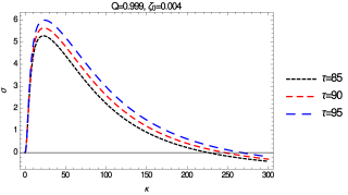
Figure 1: Plot of $\sigma_{\kappa}$ as a function of $\kappa$ from expr. (69), for fixed values $\zeta_{0}=0.004$, $Q=0.999$, and $\tau=85$ ($\varpi=62,459.5$) (black, short-dashed), $\tau=90$ ($\varpi=70,023.8$) (red, medium-dashed) and $\tau=95$ ($\varpi=78,020.3$) (blue,long- dashed). Larger values of $\tau$ allow for more unstable modes, as expected.

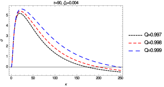
Figure 2: Plot of $\sigma_{\kappa}$ as a function of $\kappa$ from expr. (69), for fixed values $\tau=90$, $\zeta_{0}=0.004$, $Q=0.997$ ($\varpi=35,011.9$) (black, short-dashed), $Q=0.998$ ($\varpi=46,682.5$) (red, medium-dashed) and $Q=0.999$ ($\varpi=70,023.8$) (blue, long-dashed). As expected, a larger excess of particles over antiparticles allows for more unstable modes.

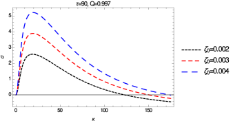
Figure 3: Plot of $\sigma_{\kappa}$ as a function of $\kappa$ from expr. (69), for fixed values $\tau=90$, $Q=0,997$ ($\varpi=35,011.9$) and $\zeta_{0}=0.002$ (black, short- dashed), $\zeta_{0}=0.003$ (red, medium-dashed) and $\zeta_{0}=0.004$ (blue, long-dashed). Again, larger values of the background anisotropy allow for more unstable modes.

One last consideration concerns the fact that the magnetic field grows when the system is in the only unstable mode. This can be seen from eq. (56), because if $F^{a3}$ would be zero, then so is $v^{a}$, and all amplitudes would vanish.

V Conclusions

In this manuscript we have built a minimal magnetohydrodynamic formalism to describe highly relativistic dissipative plasmas and their instabilities in a unified way. For consistency at microscopic and macroscopic levels, we anchored the hydrodynamics to kinetic theory by writing all tensors of the model as moments of a 1pdf, and their corresponding evolution equations as moments of a Vlasov-Boltzmann equation. For the collision integral, we used the Anderson-Witting prescription, which is a linear function of the non-equilibrium part of the 1pdf. This choice proved to describe more accurately highly relativistic systems than the BGK ansatz, as explained in Section I. We built the non-equilibrium 1pdf by introducing two new tensors, $\zeta^{\mu}$ and $\zeta^{\mu\nu}$ in such a way that the conduction currents and viscous stresses are linear on them. This simplifies the mathematics at the price of enforcing positivity of the pressures; however, the resulting formalism contains all the nonlinearities already present in the usual MHD, namely those coming from convective terms and from the coupling to the electromagnetic fields.

We applied our formalism to analyze transverse normal modes around an anisotropic background. We found a dispersion relation, eq. (69) consistent with the approximations made. This relation describes instabilities in the long wavelength range, with features that are in agreement with those found in previous works YooDav87 ; SSGT06 ; Hon04 ; Yoon07 . Our model is robust in the sense that no fine-tunning was needed to get these results.

In other words, we provided a check that pure hydrodynamic schemes are rich enough to describe the essential features of a anisotropic instabilities. We observe that there are in the literature mixed analyses in which the linearized fluctuations around an anisotropic solution to kinetic theory are described in hydrodynamic waysCJPR13 .

To the best of our knowledge, this is the first time a set of hydrodynamic equations is presented that describe both the background and the fluctuations. In last analysis, the usefulness of having a purely hydrodynamic theory is that it should make much easier to test it against experimental results, to implement numerical simulations and to follow the evolution of the instability beyond the linearized approximation ArMo06 ; RSA08 ; RS10 ; IRS11 ; ARS13b ; AKLN14 ; FIWi11 ; Fuk13 ; Khac08 ; CaRe10 . We expect to report on this last issue in the near future as well as on the extension of our formalism to non-Abelian relativistic plasmas and also a full comparison between hydrodynamic instabilities and the more detailed description that follows from kinetic theory with an Anderson-Witting collision term and-witt1 ; and-witt2 ; TI10 ; epv-2 ; SSGT06 .

References

- (1) W. Hiscock and L. Lindblom, Ann. Phys. 151 (1983) 466; Phys. Rev. D 31 (1985) 725; Contemp. Math. 71 (1988) 181.
- (2) C. Eckart, Phys. Rev. 58, 919-924 (1940).
- (3) L. D. Landau and E. M. Lifshitz, Fluid Mechanics, Pergamon Press eds, Oxford England (1959).
- (4) P. Ván and T.S. Biró, Phys. Lett. B 709, 106 (2012).
- (5) W. Israel, Covariant fluid mechanics and thermodynamics: an introduction, in Relativistic fluid dynamics, A. Anile and Y. Choquet - Bruhat (eds.), Springer, New York USA, 1988; Ann. Phys. (NY), 100, 310 (1976).
- (6) I. S. Liu, Arch. for Rat. Mech. and Anal., 46, 2, 131 (1972).
- (7) I. S. Liu, I. Müller and T. Ruggeri, Ann. of Phys., 169, 191 (1986).
- (8) R. Geroch and L. Lindblom, Phys. Rev. D, 41, 1855 (1990); ibid, Ann. Phys. (NY) 207, 394 (1991).
- (9) Thomas Schaefer, Fluid Dynamics and Viscosity in Strongly Correlated Fluids, Ann. Rev. Nucl. Part. Sci. Vol. 64 (2014) 125148, DOI: 10.1146/annurevnucl102313025439 ePrint: arXiv:1403.0653 [hepph]
- (10) Sangyong Jeon and Ulrich Heinz, Introduction to Hydrodynamics, Int. J. Mod. Phys. E Vol. 24 (2015) 1530010, DOI: 10.1142/S0218301315300106 ePrint: arXiv:1503.03931 [hepph]
- (11) P. Romatschke, arXiv:1609.02820 (2016).
- (12) L. Tinti, R. Ryblewski, W. Florkowski and M. Strickland, Nuc. Phys. A, 946 (2016).
- (13) M. Strickland, Acta Phys. Pol. B, 45, 2355 (2014).
- (14) S. Mrówczyński, B. Schenke and M. Strickland, arXiv:1603.08946 (2016).
- (15) X. G. Huang, Rep. Prog. Phys., 79, 076302 (2016).
- (16) J. Peralta-Ramos and E. Calzetta, Phys. Rev. D, 80, 126002 (2009).
- (17) J. Peralta-Ramos and E. Calzetta, Phys. Rev. C, 82, 054905 (2010).
- (18) C. Manuel and S. Mrówczyński, Phys. Rev. D, 74, 105003 (2006).
- (19) J. Peralta-Ramos and E. Calzetta, Phys. Rev. D, 86, 125024 (2012).
- (20) C. Marle, Ann. Inst. Henri Poincaré (A), 10, 67 (1969).
- (21) C. Marle, Ann. Inst. Henri Poincaré (A), 10, 127 (1969).
- (22) J. L. Anderson and H. R. Witting, Physica, 74 (1974) 466.
- (23) J. L. Anderson and H. R. Witting, Physica, 74, 489 (1974).
- (24) M. Takamoto and S. -I. Inutsuka, Physica A, 389, 4580 (2010).
- (25) M. Aguilar and E. Calzetta, in preparation (2017).
- (26) E. S. Weibel, Phys. Rev. Lett., 2, 83 (1959).
- (27) R. Schlickeiser, Phys. Plasmas, 11, 5532 (2004).
- (28) A. Achterberg and J. Wiersma, Astron. Astrophys, 475, 1 (2007).
- (29) A. Achterberg, J. Wiersma and C. A. Norman, Astron. Astrophys, 475, 19 (2007).
- (30) B. Basu, Phys. Plasmas, 9, 5131 (2002).
- (31) A. Bret and C. Deutsch, Phys. Plasmas, 13, 042106 (2006).
- (32) A. Bret, Phys. Lett. A, 359, 52 (2006).
- (33) A. Bret, Astrophys. J., 699, 990 (2009).
- (34) M. Mannarelli and C. Manuel, Phys. Rev. D, 76, 094007 (2007).
- (35) Ch. Misner, K. Thorne and J. A. Wheeler, Gravitation, Freeman, San Francisco, 1970
- (36) L. M. Martyushev and V. D. Seleznev, Phys. Rep., 426, 1 (2006).
- (37) T. Christen and F. Kassubek, J. Phys. D, 47, 363001 (2014).
- (38) T. Christen, Eur. Phys. Lett., 89, 57007 (2010).
- (39) T. Christen and F. Kassubek, J. Quant. Spectrosc. Radiat. Transf., 110, 452, (2009).
- (40) E. Calzetta and J. Peralta-Ramos, Phys. Rev. D, 82, 106003 (2010).
- (41) J. Peralta-Ramos and E. Calzetta, Phys. Rev. D, 87, 034003 (2013).
- (42) E. Calzetta, arXiv:1310.0841 (2013).
- (43) D. D. Joseph and L. Preziosi, Heat Waves, Rev. Mod. Phys. 61, 41 (1989); ibid. 62, 375 (1990)
- (44) P. H. Yoon and R. C. Davidson, Phys. Rev. A, 35, 2718 (1987).
- (45) B. Schenke, M. Strickland, C. Greiner and M. H. Thoma, Phys. Rev. D, 73, 125004 (2006).
- (46) M. Honda, Phys. Rev. E, 69, 016401 (2004).
- (47) P. H. Yoon, Phys. Plasmas, 14, 024504 (2007).
- (48) E. Calzetta and J. Peralta-Ramos, Phys. Rev. D, 88, 095010 (2013).
- (49) P. Arnold and G. D. Moore, Phys. Rev. D, 73, 025006 (2006).
- (50) A. Rebhan, M. Strickland and M. Attems, Phys. Rev. D, 78, 045023 (2008).
- (51) A. Rebhan and D. Steineder, Phys. Rev. D, 81, 085044 (2010).
- (52) A. Ipp, A. Rebhan and M. Strickland, Phys. Rev. D, 84, 056003 (2011).
- (53) M. Attems, A. Rebhan and M. Strickland, Phys. Rev. D, 87, 025010 (2013).
- (54) M. C. A. York, A. Kurkela, E. Lu and G. D. Moore, Phys. Rev. D, 89, 074036 (2014).
- (55) S. Flörchinger and U. A. Wiedemann, JHEP, 11, 100 (2011).
- (56) K. Fukushima, Phys. Rev. C, 89, 024907 (2014).
- (57) V. Khachatryan, Nuc. Phys. A, 810, 109 (2008)
- (58) M. E. Carrington and A. Rheban, Eur. Phys. J. C, 71, 1787 (2011).