Geometry of the uniform spanning forest components in high dimensions

Abstract

In this note we study the geometry of the component of the origin in the Uniform Spanning Forest of $\mathbb{Z}^{d}$, as well as in the Uniform Spanning Tree of wired subgraphs of ${\mathbb{Z}}^{d}$, when $d\geq 5$. In particular, we study connectivity properties with respect to the Euclidean and the intrinsic distance. We intend to supplement these with further estimates in the future. We are making this preliminary note available, as one of our estimates is used in work of Bhupatiraju, Hanson and Járai [BHJ] on sandpiles.

1 Introduction

The Uniform Spanning Tree (UST) on a finite graph $G$ is a random spanning tree of $G$, chosen uniformly among all spanning trees of $G$. Motivated by questions of Lyons, Pemantle [Pem91] considered the weak limit of the USTs on a growing sequence of subgraphs of ${\mathbb{Z}}^{d}$, induced by sets $V_{n}\uparrow{\mathbb{Z}}^{d}$, and showed that the limit exists. The limiting random object, that is a random spanning forest of ${\mathbb{Z}}^{d}$, is called the Uniform Spanning Forest (USF). Implicit in Pemantle’s work is the result that an alternative choice of boundary condition yields the same limit. Namely, form the “wired” graph $G_{n}^{W}=(V_{n}\cup\{r_{n}\},E_{n})$, by collapsing all vertices in ${\mathbb{Z}}^{d}\setminus V_{n}$ into $r_{n}$, and removing self-loops created at $r_{n}$. Then the weak limit of the USTs on $G_{n}^{W}$ coincides with the USF. One of Pemantle’s results was that the USF is connected a.s. in dimensions $1\leq d\leq 4$, but it consists of infinitely many (infinite) trees a.s. in dimensions $d\geq 5$.

Fundamental to the study of the UST/USF is Wilson’s algorithm [W], [LP] that allows one to build the UST/USF from Loop-Erased Random Walks (LERWs), and thereby analyze it in terms of random walk. All the necessary background about the UST/USF, that we do not detail in this note, can be found in the book [LP].

Masson [Mas] and Barlow and Masson [BM1, BM2] studied the geometry of the LERW and the UST in two dimensions. This led to a detailed understanding of random walk on the UST. The purpose of this note is to prove estimates on the geometry of the LERW and the USF in dimensions $d\geq 5$. We are interested in properties such as the length of paths and volumes of balls, both with respect to Euclidean distance and the intrinsic metric of the tree components. On the one hand we are interested in extending results from 2D to high dimensions, where the geometry is very different. On the other hand, our Theorem 5.4 is used in work of Bhupatiraju, Hanson and Járai [BHJ] on sandpiles.

2 Notation

Let ${\mathcal{U}}={\mathcal{U}}_{{\mathbb{Z}}^{d}}$ be the USF in ${\mathbb{Z}}^{d}$, viewed as a random subgraph of the nearest neighbour integer lattice. Write ${\mathcal{U}}(x)$ for the connected component of ${\mathcal{U}}$ containing $x$.

We extend this notation to $D\subset{\mathbb{Z}}^{d}$ as follows. When $D$ is finite, ${\mathcal{U}}={\mathcal{U}}_{D}$ denotes the UST on the wired graph $G_{D}^{W}=(D\cup\{r_{D}\},E_{D})$, where $E_{D}$ can be identified with those edges of ${\mathbb{Z}}^{d}$ that have at least one endpoint in $D$. For $x\in D$, we denote by ${\mathcal{U}}(x)$ the connected component of $x$ in the graph obtained from ${\mathcal{U}}$ by splitting all edges at $r_{D}$. In other words, ${\mathcal{U}}(x)$ is the union of those paths in ${\mathcal{U}}$ that do not contain $r_{D}$ as an interior vertex. We write ${\mathcal{U}}_{0}$ for ${\mathcal{U}}(0)$, when $0\in D$.

When $D\subset{\mathbb{Z}}^{d}$ is infinite, we let ${\mathcal{U}}$ denote the weak limit, as $n\rightarrow\infty$, of the USTs on the wired graphs $G_{D_{n}}^{W}$, where $D_{n}=\{x\in D:|x|\leq n\}$. The limit exists due to monotonicity; see [LP]. Wilson’s algorithm rooted at infinity [BLPS], [LP] can be easily adapted to sample ${\mathcal{U}}$. We let ${\mathcal{U}}(x)$ denote the union of those paths in ${\mathcal{U}}$ that do not contain $r_{D}$ as an interior vertex, and ${\mathcal{U}}_{0}={\mathcal{U}}(0)$.

For any of the cases of ${\mathbb{Z}}^{d}$, or $D\subset{\mathbb{Z}}^{d}$ finite or infinite, we let

$$d_{\mathcal{U}}(x,y):=\text{graph distance between $x$ and $y$ in ${\mathcal{U}}$},$$

where, if $y\not\in{\mathcal{U}}(x)$, we set $d_{\mathcal{U}}(x,y)=\infty$. The meaning of ${\mathcal{U}}$ will always be clear from context.

Notation for sets: We denote balls in different metrics as follows:

$$B_{E}(x,r) =\{y\in{\mathbb{Z}}^{d}:|x-y|\leq r\},$$

$$B_{n} =B_{E}(0,n)$$

$$Q(x,n) =\{y\in{\mathbb{Z}}^{d}:||x-y||_{\infty}\leq n\},$$

$$Q_{n} =Q(0,n),$$

$$B_{\mathcal{U}}(x,r) =\{y\in{\mathbb{Z}}^{d}:d_{\mathcal{U}}(x,y)\leq r\},$$

For $A\subset{\mathbb{Z}}^{d}$ we denote:

$$\partial A =\{x\in{\mathbb{Z}}^{d}-A:x\sim y\hbox{ for some }y\in A\},$$

$$\partial_{i}A =\{x\in A:x\sim y\hbox{ for some }y\in A^{c}\},$$

$$A^{o} =A-\partial_{i}A.$$

Let $\pi_{i}$ be projection onto the $i$th coordinate axis, and ${\mathbb{H}}_{n}$ be the hyperplane

$${\mathbb{H}}_{n}=\{x:\pi_{1}(x)=n\}.$$

Let ${\mathcal{R}}_{n}=\{n\}\times[-n,n]^{d-1}$ denote the “right-hand face” of $[-n,n]^{d}$, in the first coordinate direction.

Notation for processes. $S^{x}=(S^{x}_{k},k\geq 0)$ is simple random walk with $S^{x}_{0}=x$, and ${\mathbb{P}}^{x}$ is its law. We let $S=S^{0}$, and ${\mathbb{P}}={\mathbb{P}}^{0}$. If we discuss random walks $S^{x}$ and $S^{y}$ with $x\not=y$, then they will always be independent.

A path $\gamma$ is a (non-necessarily self avoiding) sequence of adjacent vertices in ${\mathbb{Z}}^{d}$ – ie $\gamma=(\gamma_{0},\gamma_{1},\dots)$ with $\gamma_{i-1}\sim\gamma_{i}$. (Sometimes we will write $\gamma(i)$ for $\gamma_{i}$.) Paths can be either finite or infinite. We will often need to consider the beginning or final portions of paths with respect to the first or last hit on a set. To this end, we define a number of operations on paths. Let $\gamma=(\gamma_{0},\gamma_{1},\dots)$ be a path. Given a set $A\subset{\mathbb{Z}}^{d}$ define $k_{1}=\min\{k\geq 0:\gamma_{k}\in A\}$, $k_{2}=\max\{k\geq 0:\gamma_{k}\in A\}$, and set

$${\mathcal{B}}^{F}_{A}\gamma =(\gamma_{k_{1}},\gamma_{k_{1}+1},\dots,),$$

$${\mathcal{B}}^{L}_{A}\gamma =(\gamma_{k_{2}},\gamma_{k_{1}+1},\dots,),$$

$${\mathcal{E}}^{F}_{A}\gamma =(\gamma_{0},\dots,\gamma_{k_{1}}),$$

$${\mathcal{E}}^{L}_{A}\gamma =(\gamma_{0},\dots,\gamma_{k_{2}}),$$

$$\Theta_{k}\gamma =(\gamma_{k},\dots),$$

$$\Phi_{k}\gamma =(\gamma_{0},\dots,\gamma_{k}),$$

$$H_{A}(\gamma) =\sum_{i}1_{(\gamma_{i}\in A)}.$$

Thus ${\mathcal{B}}^{F}_{A}\gamma$ is the path $\gamma$ ‘Beginning’ at the ‘First’ hit on $A$, and ${\mathcal{E}}^{L}_{A}\gamma$ is the path $\gamma$ ‘Ended’ at the ‘Last’ hit on $A$, etc. If $\gamma$ is a finite path we write $|\gamma|$ for the length of $\gamma$. $H_{A}(\gamma)$ is the number of hits by $\gamma$ on the set $A$. Let ${\mathcal{L}}\gamma$ be chronological loop erasure of $\gamma$, and if $\gamma=(\gamma_{0},\dots,\gamma_{n})$ is a finite path let ${\mathcal{R}}\gamma=(\gamma_{n},\gamma_{n-1},\dots,\gamma_{0})$ be the time reversal of $\gamma$.

We define hitting times

$$\begin{split}\tau_{A}&=\inf\{j\geq 0:S_{j}\not\in A\},\\ T_{A}&=\inf\{j\geq 0:S_{j}\in A\},\\ T_{A}^{+}&=\inf\{j\geq 1:S_{j}\in A\}.\end{split}$$

When we need to specify the process we write $T_{A}[S]$ etc.

Given a domain $D\subset{\mathbb{Z}}^{d}$, we denote the Green functions

$$\begin{split}G_{D}(x,y)&={\mathbb{E}}^{x}\Big{(}\sum_{0\leq k<\tau_{D}}I[S^{x}=y]\Big{)}\\ G(x,y)&=G_{{\mathbb{Z}}^{d}}(x,y).\end{split}$$

A note on constants. Throughout, $c$ and $C$ will denote positive finite constants that only depend on the dimension $d$, and whose value may change from line to line, and even within a single string of inequalities.

3 Properties of the LERW

In this section we derive a number of auxiliary estimates on LERW in dimensions $d\geq 5$. Some of these will be used in Sections 4 and 5, where we give upper and lower bounds on the volume of balls in the intrinsic metric. Two results of this section that are of interest in themselves are: (i) Proposition 3.11, that gives a large deviation upper bound on the lower tail of the number of steps in a LERW up to its exit from a large box; and (ii) Theorem 3.12, that gives an upper bound on the probability that $x,y\in{\mathbb{Z}}^{d}$ are in the same component of ${\mathcal{U}}$ and the path between them has length at most $n$.

The papers [Mas, BM1] give a number of properties of LERW in ${\mathbb{Z}}^{2}$, some of which hold for more general graphs.

A fundamental fact about LERWs is the following “Domain Markov property” — see [La2].

Lemma 3.1.

Let $D\subset{\mathbb{Z}}^{d}$, let $\gamma=(\gamma_{0},\dots,\gamma_{n})$ be a path from $x=\gamma_{0}$ to $D^{c}$. Set $\alpha=\Phi_{k}\gamma$, $\beta=\Theta_{k}\gamma$. Let $Y$ be a random walk started at $\gamma_{k}$ conditioned on the event $\{\tau_{D}(Y)<T^{+}_{\alpha}(Y)\}$. Then

$${\mathbb{P}}\big{(}{\mathcal{L}}({\mathcal{E}}^{F}_{D^{c}}S)=\gamma|\Psi_{k}({\mathcal{L}}({\mathcal{E}}^{F}_{D^{c}}S))=\alpha\big{)}={\mathbb{P}}({\mathcal{L}}({\mathcal{E}}^{F}_{D^{c}}Y)=\beta).$$ (3.1)

A key result in [Mas] is a ‘separation lemma’ when $d=2$ – see [Mas, Theorem 4.7]. Let $S,S^{\prime}$ be independent SRW in ${\mathbb{Z}}^{d}$ with $S_{0}=S^{\prime}_{0}=0$, and $T_{n},T^{\prime}_{n}$ be the hitting times of $\partial Q_{n}$. Set

$$F_{n} =\{S[1,T_{n}]\cap S^{\prime}[1,T^{\prime}_{n}]=\emptyset\},$$

$$Z_{n} =d(S(T_{n}),S^{\prime}[1,T^{\prime}_{n}])\vee d(S^{\prime}(T^{\prime}_{n}),S[0,T_{n}]).$$

Lemma 3.2.

(‘Separation lemma’). Let $d\geq 5$. There exists $c_{1}>0$ such that

$${\mathbb{P}}(Z_{n}\geq{\tfrac{1}{2}}n|F_{n})\geq c_{1}.$$

Proof. Let $e_{1}=(1,0,\dots,0)$. Let $X$ be a SRW started at $2ke_{1}$, and $A_{k}=\{je_{1},k\leq j\leq 2k\}$. Since $d\geq 5$ two independent SRWs intersect with probability less than 1, and thus there exists $k$ (depending on $d$) such that

$${\mathbb{P}}^{0}(\hbox{$S$ hits }X\cup A_{k})\leq\tfrac{1}{16}d^{-2}.$$

Now fix this $k$, and let

$$G_{1}=\{S_{i}=-ie_{1},S^{\prime}_{i}=ie_{1},0\leq i\leq k\}.$$

So ${\mathbb{P}}(G_{1})=(2d)^{-2k}$. Then writing $G_{2}=\{S[1,T_{n/2}]\cap S^{\prime}[1,T^{\prime}_{n/2}]\neq\emptyset\}$,

$${\mathbb{P}}(G_{2}|G_{1}) \leq{\mathbb{P}}(S[k+1,T_{n/2}]\cap S^{\prime}[1,T^{\prime}_{n/2}]\neq\emptyset|G_{1})+{\mathbb{P}}(S[1,T_{n/2}]\cap S^{\prime}[k,T^{\prime}_{n/2}]\neq\emptyset|G_{1})$$

$$\leq\tfrac{1}{8}d^{-2}.$$

Let $H_{\pm}$ be the left and right faces (in the $e_{1}$ direction) of the cube $Q_{n/2}$. We have

$${\mathbb{P}}(S_{T_{n/2}}\in H_{-}|G_{1})\geq(2d)^{-1}.$$

So if $G_{3}=G_{2}^{c}\cap\{S_{T_{n/2}}\in H_{-},S^{\prime}_{T^{\prime}_{n/2}}\in H_{+}\}$,

$${\mathbb{P}}(G_{3}|G_{1}) \geq{\mathbb{P}}(S_{T_{n/2}}\in H_{-},S^{\prime}_{T^{\prime}_{n/2}}\in H_{+}|G_{1})-{\mathbb{P}}(G_{2}|G_{1})$$

$$\geq(2d)^{-2}-(8d^{2})^{-1}=(8d^{2})^{-1}.$$

If $G_{3}$ occurs then let $G_{4}$ be the event that $S^{\prime}$ then (i.e. after time $T^{\prime}_{n/2}$ leaves $Q_{n}$ before it hits hits ${\mathbb{H}}_{0}$, and $S$ leaves $Q_{n}$ before it hits ${\mathbb{H}}_{0}$. By comparison with a one-dimensional SRW each of these events has probability at least $1/3$, so ${\mathbb{P}}(G_{4}|G_{3})\geq 1/9$. On the event $G_{1}\cap G_{3}\cap G_{4}$ the path $S[0,T_{n}]$ is contained in $[-n,0]\times[-n,n]^{d-1}\cup Q_{n/2}$, and $\pi_{1}(S^{\prime}_{T^{\prime}_{n}}=n)$, so that $d(S^{\prime}_{T^{\prime}_{n}},S[0,T_{n}])\geq n/2$. The same bound holds if we interchange $S^{\prime}$ and $S$, and so we deduce that

$${\mathbb{P}}(Z_{n}\geq{\tfrac{1}{2}}n|F_{n})\geq{\mathbb{P}}(\{Z_{n}\geq{\tfrac{1}{2}}n\}\cap F_{n})\geq{\mathbb{P}}(G_{1}\cap G_{3}\cap G_{4})\geq(2d)^{-2k}(8d^{2})^{-1}9^{-1}.$$

$\square$

Remark. The result in $d\geq 5$ is much easier than $d=2$, since with high probability $S$ and $S^{\prime}$ do not interesect. The proof for $d=2$ uses the fact that if the two processes get too close, then by the Beurling estimate they hit with high probability.

In the remainder of this section we give some estimates on the length of LERW paths in ${\mathbb{Z}}^{d}$ with $d\geq 5$. We fix $D\subset{\mathbb{Z}}^{d}$ and $N\geq 1$ such that $Q_{N}=Q(0,N)\subset D$. We will be interested in the number of steps the LERW from $0$ to $\partial D$ takes up to its first exit from $Q_{N}$. Let $S$ be SRW on ${\mathbb{Z}}^{d}$ with $S_{0}=0$. Let

$$L={\mathcal{L}}({\mathcal{E}}^{F}_{D^{c}}(S)).$$

In words, $L$ is the loop erasure of $S$ up to its first hit on the boundary of $D$.

Our estimate will be broken down into studying $L$ in ‘shells’ $Q_{n+m}\setminus Q_{n}$. For this purpose, let us fix $n,m$ such that $16\leq n<n+m\leq N$, with $m\leq n/8$. Let

$$\alpha={\mathcal{E}}^{F}_{\partial_{i}Q_{n}}L,\quad L^{\prime}={\mathcal{B}}^{F}_{\partial_{i}Q_{n}}L.$$

So $\alpha$ is the path $L$ up to its first hit on $\partial_{i}Q(0,n)$, and $L^{\prime}$ is the path of $L$ from this time on. See Figure 1.

Let us condition on $\alpha$. Let $x_{0}\in\partial_{i}Q_{n}$ be the endpoint of $\alpha$. When $x_{0}\in{\mathbb{H}}_{n}$, we let $x_{1}=x_{0}+(m/2)e_{1}$ and set

$$A=A(x_{0})=Q(x_{1},m/4),\quad,A^{*}=Q(x_{1},3m/8).$$

When $x_{0}$ lies on one of the other faces of $Q_{n}$, we replace $e_{1}$ by the unit vector pointing towards that faces to define $x_{1}$ and $A(x_{0})$. See Figure 1.

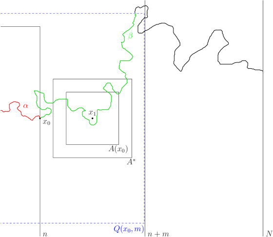
Figure 1: Setup and notation for the piece of the LERW in the shell $Q_{n+m}\setminus Q_{n}$.

Set

$$\beta={\mathcal{E}}^{F}_{\partial_{i}Q(x_{0},m)}L^{\prime}.$$

Let $\widetilde{X}^{z}$ be $S^{z}$ conditioned on $\{\tau_{D}<T^{+}_{\alpha}\}$. While the process $\widetilde{X}^{z}$ depends on $\alpha$, our notation will not emphasize this point. Write $\widetilde{X}$ for $\widetilde{X}^{x_{0}}$, and $\widetilde{G}_{D}(x,y)$ for the Green function for $\widetilde{X}^{x}$. By the domain Markov property, Lemma 3.1, we have (conditional on $\alpha$) that

$$L^{\prime}\,\,{\buildrel(d)\over{=}}\,\,{\mathcal{L}}({\mathcal{E}}^{F}_{\partial D}\widetilde{X}).$$ (3.2)

We write $\widetilde{T}$, $\widetilde{\tau}$, etc. for hitting and exit times by $\widetilde{X}$. Set

$$h(x)={\mathbb{P}}^{x}(\tau_{D}<T_{\alpha}).$$

Then

$$\widetilde{G}_{D}(x,y)=\frac{h(y)}{h(x)}G_{D}(x,y),\,x,y\in D-\alpha.$$ (3.3)

The standard Harnack inequality (see [La2]) gives

$$h(y)\asymp h(x_{1}),\quad y\in A^{*},$$ (3.4)

and thus

$$\widetilde{G}_{D}(x,y)\asymp G_{D}(x,y),\,x,y\in A^{*}.$$ (3.5)

Lemma 3.3.

Let $d\geq 3$. For any $\alpha$ we have

$${\mathbb{E}}(H_{A}(\beta)|\alpha) \leq c_{1}m^{2},$$ (3.6)

$${\mathbb{E}}(H_{A}(\beta)^{2}|\alpha) \leq c_{1}m^{4}.$$ (3.7)

Proof. This is a standard computation with Green functions. Let $B=Q(x_{0},m)$. Then, since $\beta$ is a subset of the path of $\widetilde{X}$, we have

$$H_{A}(\beta)\leq\sum_{k=0}^{\widetilde{\tau}_{B}}1_{(\widetilde{X}\in A)}=H_{A}({\mathcal{E}}^{F}_{\partial_{i}B}\widetilde{X})=:\widetilde{H}.$$

Then for $p=1,2$,

$${\mathbb{E}}^{x_{0}}(\widetilde{H}^{p}|\alpha)={\mathbb{E}}^{x_{0}}\Big{(}1_{(\widetilde{T}_{A^{*}}<\widetilde{\tau}_{B})}{\mathbb{E}}^{\widetilde{X}_{\widetilde{T}_{A^{*}}}}({\widetilde{H}}^{p})\Big{)}\leq\max_{z\in\partial_{i}A^{*}}{\mathbb{E}}^{z}\widetilde{H}^{p}.$$

Let $z\in\partial_{i}A^{*}$. Then using (3.5)

$${\mathbb{E}}^{z}(\widetilde{H}|\alpha) =\sum_{y\in A}\widetilde{G}_{B}(z,y)\leq c|A|\max_{y\in A}G_{B}(z,y)\leq c^{\prime}m^{2}m^{2-d}=c^{\prime}m^{2}.$$

Also since on $A^{*}$ we have $\widetilde{G}_{B}\asymp G_{B}\leq G$,

$${\mathbb{E}}^{z}(\widetilde{H}^{2}|\alpha) \leq 2\sum_{k=0}^{\infty}\sum_{k=j}^{\infty}1_{(k\leq\widetilde{\tau}_{B})}1_{(j\leq\widetilde{\tau}_{B})}1_{(\widetilde{X}_{k}\in A)}1_{(\widetilde{X}_{j}\in A)}$$

$$\leq 2\sum_{x\in A}\sum_{y\in A}\widetilde{G}_{B}(z,x)\widetilde{G}_{B}(x,y)$$

$$\leq c|A|m^{2-d}\max_{x\in A}\sum_{y\in A}\widetilde{G}(x,y)\leq c^{\prime}m^{4}.$$

$\square$

Remark 3.4.

The same argument works if we consider ${\mathbb{E}}(H_{Q(x_{1},\lambda m)}(\beta)^{p}|\alpha)$, $p=1,2$, for any $\lambda\in(0,\frac{1}{2})$.

We now turn to the harder problem of obtaining a lower bound on ${\mathbb{E}}H_{A}(\beta)$, and begin with a boundary Harnack inequality which extends [Mas, Proposition 3.5] to higher dimensions. See [BK] for further extensions. In what follows ${\mathcal{R}}_{m}={\mathbb{H}}_{m}\cap Q_{m}$ is the ‘right hand face’ of $Q_{m}$.

Lemma 3.5.

Assume $d\geq 1$. Let ${\mathcal{K}}$ be an arbitrary nonempty subset of $[-m+1,0]\times[-m+1,m-1]^{d-1}$. For all $m\geq 1$ and all ${\mathcal{K}}$ we have

$${\mathbb{P}}^{0}\big{(}S(\tau_{Q(0,m-1)})\in{\mathcal{R}}_{m}\,\big{|}\,\tau_{Q(0,m-1)}<T^{+}_{\mathcal{K}}\big{)}\geq(2d)^{-1}.$$ (3.8)

Proof. Let $h(z)={\mathbb{P}}^{z}\big{(}S_{\tau_{Q(0,m-1)}}\in{\mathcal{R}}_{m}\big{)}$, $z\in Q(0,m-1)$. By symmetry we have $h(0)=1/2d$. We first show that

$$h(z)\leq h(0)\text{ for all $z\in([-m+1,0]\times[-m+1,m-1]^{d-1})\cap{\mathbb{Z}}^{d}$}.$$ (3.9)

Let $z^{\prime}=(0,z_{2},\dots,z_{d})$. Let $X^{z}$ and $X^{z^{\prime}}$ be simple random walks with starting points $z$ and $z^{\prime}$ respectively; we have $h(z)={\mathbb{P}}(X^{z}_{\tau_{A}}\in{\mathcal{R}}_{n})$, with a similar expression for $h(z^{\prime})$. We couple these random walks by taking $X^{z}=z+S$, $X^{z^{\prime}}=z^{\prime}+S$, where $S$ is a SRW with $S_{0}=0$. Then $\{X^{z}_{\tau_{A}}\in{\mathcal{R}}_{n}\}\subset\{X^{z^{\prime}}_{\tau_{A}}\in{\mathcal{R}}_{n}\}$, and so $h(z)\leq h(z^{\prime})$.

To prove that $h(z^{\prime})\leq h(0)$ we use a coupling of continuous time random walks $Y$, $Y^{\prime}$ with $Y_{0}=0$, $Y^{\prime}_{0}=z^{\prime}$; these have the same exit distribution as the discrete time walk $S$. Recall that $\pi_{j}$ is the projection onto the $j$th coordinate axis, so that $\pi_{j}(Y_{t})$ gives the $j$th coordinate of $Y_{t}$; each coordinate is a continuous time simple random walk (run at rate $1/d$) on ${\mathbb{Z}}$.

The coupling is as follows. If at time $t$ we have $\pi_{j}(Y_{t})=\pi_{j}(Y^{\prime}_{t})$ then we run the two $j$th coordinate processes together, so $\pi_{j}(Y_{t+s})=\pi_{j}(Y^{\prime}_{t+s})$ for all $s\geq 0$

Note that we have $|\pi_{j}(Y_{t})|\leq|\pi_{j}(Y^{\prime}_{t})|$ when $t=0$; the coupling will preserve this inequality for all $t\geq 0$. If $|\pi_{j}(Y_{t})-\pi_{j}(Y^{\prime}_{t})|\geq 2$ then we use reflection coupling, so that $\pi_{j}(Y_{t})$ and $\pi_{j}(Y^{\prime}_{t})$ jump at the same time, and in opposite directions. Finally, suppose that $|\pi_{j}(Y_{t})-\pi_{j}(Y^{\prime}_{t})|=1$, and let $a=\pi_{j}(Y_{t})$, $a+1=\pi_{j}(Y^{\prime}_{t})$. We take three independent Poisson processes on ${\mathbb{R}}_{+}$, ${\mathcal{P}}_{1},{\mathcal{P}}_{2},{\mathcal{P}}_{3}$; each with rate $1/2d$, and make the first jump of either $\pi_{j}(Y)$ or $\pi_{j}(Y^{\prime})$ after time $t$ to be at time $t+T$, where $T$ is the first point in ${\mathcal{P}}_{1}\cup{\mathcal{P}}_{2}\cup{\mathcal{P}}_{3}$. If $T\in{\mathcal{P}}_{1}$ we set $\pi_{j}(Y_{t+T})=a-1$, $\pi_{j}(Y^{\prime}_{t+T})=a+2$. If $T\in{\mathcal{P}}_{2}$ then we set $\pi_{j}(Y_{t+T})=a+1$, $\pi_{j}(Y^{\prime}_{t+T})=a+1$, and if $T\in{\mathcal{P}}_{3}$ then $\pi_{j}(Y_{t+T})=a$, $\pi_{j}(Y^{\prime}_{t+T})=a$. With this coupling we have $\{Y^{\prime}_{\tau_{A}(Y^{\prime})}\in{\mathcal{R}}_{n}\}\subset\{Y_{\tau_{A}(Y)}\in{\mathcal{R}}_{n}\}$, and so $h(z^{\prime})\leq h(0)$.

Stopping the bounded martingale $h(S(k))$ at $\tau_{Q(0,m-1)}\wedge T_{\mathcal{K}}$, and using (3.9) we get

$$\begin{split}h(0)&=\sum_{y\in{\mathcal{K}}}h(y){\mathbb{P}}^{0}\big{(}S(\tau_{Q(0,m-1)}\wedge T^{+}_{\mathcal{K}})=y\big{)}+{\mathbb{P}}^{0}\big{(}\tau_{Q(0,m-1)}<T^{+}_{\mathcal{K}},\,S(\tau_{Q(0,m-1)})\in{\mathcal{R}}_{m}\big{)}\\ &\leq h(0){\mathbb{P}}\big{(}\tau_{Q(0,m-1)}>T^{+}_{\mathcal{K}})+{\mathbb{P}}(\tau_{Q(0,m-1)}<T^{+}_{\mathcal{K}},\,S(\tau_{Q(0,m-1)})\in{\mathcal{R}}_{m}\big{)}.\end{split}$$

Rearranging gives the statement of the lemma. $\square$

We will also need two extensions of Lemma 3.5 that we prove next.

Lemma 3.6.

Assume $d\geq 3$. Let $N\geq 1$ and $Q_{4N}\subset D\subset{\mathbb{Z}}^{d}$. Let $8\leq m\leq N/2$ and $n\leq N$. Suppose that ${\mathcal{K}}$ is an arbitrary nonempty subset of $Q_{n}$, and $x_{0}\in{\mathcal{K}}\cap{\mathbb{H}}_{n}$. Let $z_{0}=x_{0}+me_{1}$. There exists a constant $c=c(d)>0$ such that

$${\mathbb{P}}^{z_{0}}(T_{Q(x_{0},m/2)}>\tau_{D}\,|\,T_{{\mathcal{K}}}>\tau_{D})\geq c.$$ (3.10)

Proof. It is easy to see that the statement holds when $m\geq n/8$, since then ${\mathbb{P}}^{z_{0}}(T_{Q_{n+m/2}}>\tau_{D})\geq{\mathbb{P}}^{z_{0}}(T_{Q_{n+m/2}}=\infty)\geq c$. Henceforth we assume that $m<n/8$.

Let $f(z)={\mathbb{P}}^{z}(T_{{\mathcal{K}}}>\tau_{D})$ and $g(z)={\mathbb{P}}^{z}(T_{{\mathcal{K}}}\wedge T_{Q(x_{0},m/2)}>\tau_{D})$, so that we have to prove $f(z_{0})\leq Cg(z_{0})$. Let $z_{1}=x_{0}+8me_{1}$. Due to the Harnack principle, it is sufficient to show that $f(z_{1})\leq Cg(z_{1})$.

We first show that for all $y\in\partial Q(x_{0},8m)$ we have $g(y)\leq Cg(z_{1})$. Let us write ${\mathbb{H}}$ for the hyperplane ${\mathbb{H}}_{n+4m}$, and ${\mathbb{H}}^{\prime}$ for the hyperplane ${\mathbb{H}}_{n+2m}$. Observe that ${\mathbb{H}}$ and ${\mathbb{H}}^{\prime}$ are both disjoint from ${\mathcal{K}}\cup Q(x_{0},m/2)$, and they both separate ${\mathcal{K}}\cup Q(x_{0},m/2)$ from $z_{1}$.

If $y\in\partial Q(x_{0},8m)$ lies on the same side of ${\mathbb{H}}^{\prime}$ as $z_{1}$, then $y$ is at least distance $m$ from ${\mathcal{K}}\cup Q(x_{0},m/2)$, and this is comparable to the distance between $y$ and $z_{1}$. Hence for such $y$, the Harnack principle implies $g(y)\leq Cg(z_{1})$.

Suppose now that ${\mathbb{H}}^{\prime}$ separates $y$ from $z_{1}$. Let $Q^{(1)}$ and $Q^{(2)}$ be cubes that are both translates of $Q_{2N}$, such that:
(i) the right hand face of $Q^{(1)}$ and the left hand face of $Q^{(2)}$ coincide;
(ii) the common set $\mathcal{R}=Q^{(1)}\cap Q^{(2)}$, is contained in ${\mathbb{H}}$;
(iii) the center of $\mathcal{R}$ (viewed as a $(d-1)$-dimensional cube), is the point $x_{0}+4me_{1}$.
Since $g(S(n\wedge\tau_{Q^{(1)}}))$ is a submartingale under ${\mathbb{P}}^{y}$, we have

$$g(y)\leq{\mathbb{E}}^{y}(g(\tau_{Q^{(1)}}))=\sum_{w\in\partial Q^{(1)}\setminus\mathcal{R}}g(w)\,{\mathbb{P}}^{y}(S(\tau_{Q^{(1)}})=w)+\sum_{u\in\mathcal{R}}g(u)\,{\mathbb{P}}^{y}(S(\tau_{Q^{(1)}})=u).$$ (3.11)

Since $g(S(n\wedge\tau_{Q^{(2)}}))$ is a martingale under ${\mathbb{P}}^{z_{1}}$, we also have

$$g(z_{1})={\mathbb{E}}^{z_{1}}(g(\tau_{Q^{(2)}}))=\sum_{w^{\prime}\in\partial Q^{(2)}\setminus\mathcal{R}}g(w^{\prime})\,{\mathbb{P}}^{z_{1}}(S(\tau_{Q^{(2)}})=w^{\prime})+\sum_{u\in\mathcal{R}}g(u)\,{\mathbb{P}}^{z_{1}}(S(\tau_{Q^{(2)}})=u).$$ (3.12)

The mirror symmetry between $Q^{(1)}$ and $Q^{(2)}$, as well as the Harnack principle implies that

$$\begin{split}{\mathbb{P}}^{y}(S(\tau_{Q^{(1)}})=u)&\leq C{\mathbb{P}}^{z_{1}}(S(\tau_{Q^{(2)}})=u)\\ {\mathbb{P}}^{y}(S(\tau_{Q^{(1)}})=w)&\leq C{\mathbb{P}}^{z_{1}}(S(\tau_{Q^{(2)}})=w^{\prime}),\end{split}$$

where $w^{\prime}$ is the mirror image of $w\in\partial Q^{(1)}\setminus\mathcal{R}$ in the hyperplane ${\mathbb{H}}$. We also have $g(w)\leq 1$, $w\in\partial Q^{(1)}\setminus\mathcal{R}$, and $g(w^{\prime})\geq c$, $w^{\prime}\in\partial Q^{(2)}$. These observations and (3.11) and (3.12) together imply $g(y)\leq Cg(z_{1})$.

We now show the desired inequality $f(z_{1})\leq Cg(z_{1})$. Let $1\leq R<\infty$ denote the random variable that counts the number of times $S^{z_{1}}$ makes a crossing from $\partial Q(x_{0},8m)$ to $Q(x_{0},m/2)$ before $T_{\mathcal{K}}\wedge\tau_{D}$. We have

$${\mathbb{P}}^{z_{1}}(R\geq\ell)\leq\left(\max_{y\in\partial Q(x_{0},8m)}{\mathbb{P}}^{y}(T_{Q(x_{0},m/2)}<\infty)\right)^{\ell}\leq\gamma^{\ell}$$

with some $0<\gamma=\gamma(d)<1$.

Using the strong Markov property at the time when the $\ell$-th crossing has occurred, we can write

$$\begin{split}f(z_{1})&=\sum_{\ell=0}^{\infty}{\mathbb{P}}^{z_{1}}(R=\ell,\,T_{\mathcal{K}}>\tau_{D})=g(z_{1})+\sum_{\ell=1}^{\infty}{\mathbb{P}}^{z_{1}}(R=\ell,\,T_{\mathcal{K}}>\tau_{D})\\ &\leq g(z_{1})+\sum_{\ell=1}^{\infty}{\mathbb{P}}^{z_{1}}(R\geq\ell)\,\max_{z\in Q(x_{0},m/2)}{\mathbb{P}}^{z}((T_{Q(x_{0},m/2)}\wedge T_{\mathcal{K}})\circ\Theta_{\tau_{Q(x_{0},8m)}}>\tau_{D})\\ &\leq g(z_{1})+\sum_{\ell=1}^{\infty}\gamma^{\ell}\max_{y\in\partial Q(x_{0},8m)}g(y)\\ &\leq g(z_{1})+Cg(z_{1}).\end{split}$$

This completes the proof of the Lemma.

Lemma 3.7.

Assume $d\geq 3$. Let $N\geq 1$ and $Q_{4N}\subset D\subset{\mathbb{Z}}^{d}$. Let $8\leq m\leq N/2$ and $n\leq N$. Suppose that ${\mathcal{K}}$ is an arbitrary nonempty subset of $Q_{n}$, and $x_{0}\in{\mathcal{K}}\cap{\mathbb{H}}_{n}$. Let $\mathcal{R}_{n,m}$ denote the right hand face of $Q(x_{0},m)$. There exists a constant $c=c(d)>0$ such that

$${\mathbb{P}}^{x_{0}}\big{(}S(\tau_{Q(x_{0},m)})\in\mathcal{R}_{n,m}\,\big{|}\,T^{+}_{\mathcal{K}}>\tau_{D}\big{)}\geq c.$$ (3.13)

Proof. Let ${\mathcal{K}}_{0}={\mathcal{K}}\cap Q(x_{0},2m)$ and ${\mathcal{K}}_{1}={\mathcal{K}}\setminus{\mathcal{K}}_{0}={\mathcal{K}}\setminus Q(x_{0},2m)$. Due to the boundary Harnack inequality, Lemma 3.5, we have

$${\mathbb{P}}^{x_{0}}\big{(}S(\tau_{Q(x_{0},m)}\in\mathcal{R}_{n,m}\,\big{|}\,T^{+}_{\mathcal{K}}>\tau_{Q(x_{0},m)}\big{)}\geq(2d)^{-1}.$$ (3.14)

Let $Z$ denote the process that is $S$ conditioned on $T_{{\mathcal{K}}_{1}}>\tau_{D}$. Then (3.14) and an application of the Harnack principle implies that

$${\mathbb{P}}^{x_{0}}\big{(}Z(\tau_{Q(x_{0},m)}\in\mathcal{R}_{n,m}\,\big{|}\,T^{+}_{\mathcal{K}}[Z]>\tau_{Q(x_{0},m)}[Z]\big{)}\geq c.$$ (3.15)

This in turn implies that

$$\begin{split}&{\mathbb{P}}^{x_{0}}\big{(}S(\tau_{Q(x_{0},m)})\in\mathcal{R}_{n,m},\,T^{+}_{\mathcal{K}}>\tau_{Q(x_{0},m)},\,T_{{\mathcal{K}}_{1}}>\tau_{D}\big{)}\\ &\qquad\geq c{\mathbb{P}}^{x_{0}}\big{(}T^{+}_{\mathcal{K}}>\tau_{Q(x_{0},m)},\,T_{{\mathcal{K}}_{1}}>\tau_{D}\big{)}\\ &\qquad\geq c{\mathbb{P}}^{x_{0}}\big{(}T^{+}_{\mathcal{K}}>\tau_{D}\big{)}.\end{split}$$ (3.16)

Let $z_{0}=x_{0}+4me_{1}$. Using the Harnack principle, the left hand side of (LABEL:e:cond-ubh) can be bounded from above by

$$\begin{split}&{\mathbb{P}}^{x_{0}}\big{(}S(\tau_{Q(x_{0},m)})\in\mathcal{R}_{n,m},\,T^{+}_{{\mathcal{K}}}>\tau_{Q(x_{0},m)}\big{)}\,\max_{z\in\mathcal{R}_{n,m}}{\mathbb{P}}^{z}\big{(}T_{{\mathcal{K}}_{1}}>\tau_{D}\big{)}\\ &\qquad\leq C\,{\mathbb{P}}^{x_{0}}\big{(}S(\tau_{Q(x_{0},m)})\in\mathcal{R}_{n,m},\,T^{+}_{{\mathcal{K}}}>\tau_{Q(x_{0},m)}\big{)}\,{\mathbb{P}}^{z_{0}}\big{(}T_{{\mathcal{K}}_{1}}>\tau_{D}\big{)}.\end{split}$$ (3.17)

An application of Lemma 3.6 (with $2m$ playing the role of $m/2$) shows that

$${\mathbb{P}}^{z_{0}}\big{(}T_{{\mathcal{K}}_{1}}>\tau_{D}\big{)}\leq C\,{\mathbb{P}}^{z_{0}}\big{(}T_{{\mathcal{K}}_{1}\cup Q(x_{0},2m)}>\tau_{D}\big{)}\leq C\,{\mathbb{P}}^{z_{0}}\big{(}T_{{\mathcal{K}}}>\tau_{D}\big{)}.$$

Substituting this into (LABEL:e:away), and using the Harnack principle again, we get that the right hand side of (LABEL:e:away) is bounded above by

$$\begin{split}&C\,{\mathbb{P}}^{x_{0}}\big{(}S(\tau_{Q(x_{0},m)})\in\mathcal{R}_{n,m},\,T^{+}_{{\mathcal{K}}}>\tau_{Q(x_{0},m)}\big{)}\,{\mathbb{P}}^{z_{0}}\big{(}T_{{\mathcal{K}}}>\tau_{D}\big{)}\\ &\qquad\leq C\,{\mathbb{P}}^{x_{0}}\big{(}S(\tau_{Q(x_{0},m)})\in\mathcal{R}_{n,m},\,T^{+}_{{\mathcal{K}}}>\tau_{Q(x_{0},m)}\big{)}\,\min_{z\in\mathcal{R}_{n,m}}{\mathbb{P}}^{z}\big{(}T_{{\mathcal{K}}}>\tau_{D}\big{)}\\ &\qquad\leq C\,{\mathbb{P}}^{x_{0}}\big{(}S(\tau_{Q(x_{0},m)})\in\mathcal{R}_{n,m},\,T^{+}_{{\mathcal{K}}}>\tau_{D}\big{)}.\end{split}$$ (3.18)

The inequalities (LABEL:e:cond-ubh), (LABEL:e:away) and (LABEL:e:bound-away) together imply the claim of the Lemma.

We now return to the task of giving a lower bound for ${\mathbb{E}}(H_{A}(\beta))$. We will need the following lower bound on $\widetilde{G}$.

Lemma 3.8.

Assume $d\geq 3$. Let $z\in A$. Then

$$\widetilde{G}_{D}(x_{0},z)\geq cm^{2-d}.$$

Proof. This uses the extension of the boundary Harnack inequality, Lemma 3.7. Let $V_{z}$ be the number of hits on $z$ by $\widetilde{X}$ before $\widetilde{\tau}_{D}$. Let $\widetilde{T}=\widetilde{T}_{\partial_{i}Q(x_{0},m/8)}$. Note that $Q(x_{0},m/8)$ and $A^{*}$ intersect on one of the faces of $Q(x_{0},m/8)$. Then since $\widetilde{T}<\widetilde{\tau}_{D}$,

$$\widetilde{G}_{D}(x_{0},z) ={\mathbb{E}}^{x_{0}}V_{z}={\mathbb{E}}^{x_{0}}\Big{(}{\mathbb{E}}^{\widetilde{X}_{\widetilde{T}}}V_{z}\Big{)}\geq{\mathbb{E}}^{x_{0}}\Big{(}1_{(\widetilde{X}_{\widetilde{T}}\in A^{*})}\min_{y\in\partial_{i}A^{*}}{\mathbb{E}}^{y}V_{z}\Big{)}$$

$$={\mathbb{P}}^{x_{0}}(\widetilde{X}_{\widetilde{T}}\in A^{*})\min_{y\in\partial_{i}A^{*}}\widetilde{G}_{D}(y,z).$$

Using (3.3) and (3.4) we have $\widetilde{G}_{D}(y,z)\asymp G_{D}(y,z)\asymp m^{2-d}$ if $y\in\partial_{i}A^{*}$. Let $T=T_{\partial_{i}Q(x_{o},m/8)}$ (for $S$). Lemma 3.7 implies

$${\mathbb{P}}^{x_{0}}(\widetilde{X}_{\widetilde{T}}\in A^{*})={\mathbb{P}}^{x_{0}}(S_{T}\in A^{*}|T^{+}_{\alpha}>\tau_{D})\geq c,$$

and the Lemma follows. $\square$

The key estimate is the following.

Lemma 3.9.

Assume $d\geq 5$. Then

$${\mathbb{E}}(H_{A}(\beta)|\alpha)\geq cm^{2}.$$ (3.19)

Proof. It is enough to prove that if $z\in A$ then

$${\mathbb{P}}(z\in\beta|\alpha)\geq cm^{2-d}.$$ (3.20)

Let $Y$ be $\widetilde{X}$ conditioned to hit $z$ before $\widetilde{T}^{+}_{\alpha}\wedge\widetilde{\tau}_{D}$, and let $\widetilde{X}^{z}$ be independent of $Y$. Let

$$Y^{\prime}={\mathcal{E}}^{L}_{z}({\mathcal{E}}^{F}_{\partial D}(Y)),$$

so $Y^{\prime}$ is the path of $Y$ up to its last hit on $z$ before its first exit from $D$. Let also $X^{\prime}=\Theta_{1}{\mathcal{E}}^{F}_{\partial D}\widetilde{X}^{z}$. (We need to apply $\Theta_{1}$ since the last point of $Y^{\prime}$ and the first point of $X^{\prime}$ are both $z$.) Then as in Lemma 6.1 of [BM1] we have

$${\mathbb{P}}(z\in\beta|\alpha)=\widetilde{G}_{D}(x_{0},z){\mathbb{P}}\big{(}{\mathcal{L}}Y^{\prime}\cap X^{\prime}=\emptyset,{\mathcal{L}}Y^{\prime}\subset Q(x_{0},m)\big{)}.$$ (3.21)

Due to Lemma 3.8, it remains to show that the probability on the right hand side is bounded away from $0$. We will in fact prove the stronger statement:

$${\mathbb{P}}\big{(}Y^{\prime}\cap X^{\prime}=\emptyset,Y^{\prime}\subset Q(x_{0},m)\big{)}\geq c>0.$$ (3.22)

This result is not surprising, since two independent SRW in ${\mathbb{Z}}^{d}$ (with $d\geq 5$) intersect with probability strictly less than 1.

Let us denote $A_{z}=Q(z,m/16)$, $B=Q(x_{0},m)$ and $B^{\prime}=Q(x_{0},m/16)$. Note that $Y^{\prime}$ starts at $x_{0}$ and ends at $z$. We decompose $Y^{\prime}$ into four subpaths, defined below, and give separate estimates for these subpaths that together will imply the lower bound on the probability in (3.22). We define:

$$\begin{split}Y^{\prime}_{1}={\mathcal{E}}^{F}_{\partial B^{\prime}}(Y^{\prime})\qquad Y^{\prime}_{2}={\mathcal{E}}^{L}_{\partial A_{z}}({\mathcal{B}}^{F}_{\partial B^{\prime}}(Y^{\prime}))\qquad Y^{\prime}_{3}={\mathcal{B}}^{L}_{\partial A_{z}}(Y^{\prime}).\end{split}$$

That is, $Y^{\prime}_{1}$ ends at the first exit from $B^{\prime}$, $Y^{\prime}_{3}$ begins at the last entrance to $A_{z}$ and $Y^{\prime}_{2}$ is the portion in between. We let $y_{1}=Y^{\prime}_{1}(|Y^{\prime}_{1}|)=Y^{\prime}_{2}(0)$ and $y_{2}=Y^{\prime}_{2}(|Y^{\prime}_{2}|)=Y^{\prime}_{3}(0)$. We further decompose $Y^{\prime}_{2}$ into the pieces:

$$\begin{split}Y^{\prime}_{2,1}={\mathcal{E}}^{F}_{y_{2}}(Y^{\prime}_{2})\qquad Y^{\prime}_{2,2}={\mathcal{B}}^{F}_{y_{2}}(Y^{\prime}_{2}).\end{split}$$

That is, $Y^{\prime}_{2,1}$ is the piece from $y_{1}$ to the first hit on $y_{2}$, and $Y^{\prime}_{2,2}$ is the remaining loop at $y_{2}$. Observe that conditional on $y_{1}$ and $y_{2}$, the paths $Y^{\prime}_{1},Y^{\prime}_{2,1},Y^{\prime}_{2,2},Y^{\prime}_{3}$ are independent. We now state our estimates for each piece. Our notation will assume that $x_{0}\in{\mathbb{H}}_{n}$; trivial modification can be made when this is not the case.

Claim 1. There is constant probability that $Y^{\prime}_{1}$ exits $B^{\prime}$ on the right hand face. That is, we have ${\mathbb{P}}(y_{1}\in\mathcal{R}_{n,m/16})\geq c>0$, where $\mathcal{R}_{n,m/16}={\mathbb{H}}_{n+m/16}\cap Q(x_{0},m/16)$.

Proof of Claim 1. Using Lemma 3.7 we have

$$\begin{split}{\mathbb{P}}(y_{1}\in\mathcal{R}_{n,m/16})&=\frac{{\mathbb{P}}^{x_{0}}(\widetilde{X}(\widetilde{\tau}_{B^{\prime}})\in\mathcal{R}_{n,m/16},\,\widetilde{T}_{z}<\widetilde{\tau}_{D})}{{\mathbb{P}}^{x_{0}}(\widetilde{T}_{z}<\widetilde{\tau}_{D})}\\ &\geq\frac{\widetilde{G}_{D}(z,z)}{\widetilde{G}_{D}(x_{0},z)}\,{\mathbb{P}}^{x_{0}}(\widetilde{X}(\widetilde{\tau}_{B^{\prime}})\in\mathcal{R}_{n,m/16})\,\min_{w\in\mathcal{R}_{n,m/16}}{\mathbb{P}}^{w}(\widetilde{T}_{z}<\tau_{D})\\ &\geq c\min_{w\in\mathcal{R}_{n,m/16}}\frac{\widetilde{G}_{D}(w,z)}{\widetilde{G}_{D}(x_{0},z)}\geq c.\end{split}$$

In the next three claims we will use the notation $B^{\prime\prime}=x_{0}+([0,z_{1}+m/32]\times[-m,m]^{d-1})\cap{\mathbb{Z}}^{d}$.

Claim 2. There is constant probability that the following six events occur:
(i) $Y^{\prime}_{3}$ starts on the left hand face of $A_{z}$;
(ii) $Y^{\prime}_{3}\subset z+([-m/16,m/32]\times[-m/16,m/16]^{d-1})\cap{\mathbb{Z}}^{d}$;
(iii) $X^{\prime}$ exits $A_{z}$ on the right hand face;
(iv) $X^{\prime}\cap A_{z}\subset z+([-m/32,m/16]\times[-m/16,m/16]^{d-1})\cap{\mathbb{Z}}^{d}$;
(v) $Y^{\prime}_{3}\cap(X^{\prime}\cap A_{z})=\emptyset$;
(vi) ${\mathcal{B}}^{F}_{\partial A_{z}}(X^{\prime})$ is disjoint from $B^{\prime\prime}$.

Proof of Claim 2. Let $\widetilde{S}^{z}$ be the process defined as $S^{z}$ conditioned to hit on $x_{0}$ before $T_{\alpha\setminus\{x_{0}\}}\wedge\tau_{D}$. The time-reversal of $Y^{\prime}$ has the law of $\widetilde{S}^{z}$. Therefore, the time-reversal of $Y^{\prime}_{3}$ has the law of ${\mathcal{E}}^{F}_{\partial A_{z}}(\widetilde{S}^{z})$. The proof of Lemma 3.2 (Separation Lemma), shows that for independent simple random walks $S^{z}$ and $S^{\prime z}$ there is probability $\geq c>0$ that the analogues of the events (i)–(v) all hold. An application of the Harnack principle then shows that in fact (i)–(v) hold with constant probability.

It is left to show that conditionally on (i)–(v), we also have (vi) with constant probability. Since $X^{\prime}$ is $S$ conditioned on $T_{\alpha}>\tau_{D}$, this can be proved in the same way as Lemma 3.6. For this we merely have to replace $Q(x_{0},m/2)$ in that lemma by $B^{\prime\prime}$, and make straightforward adjustments. Hence Claim 2 follows.

Claim 3. Conditional on $y_{1}$ being in the right hand face of $B^{\prime}$ and $y_{2}$ being in the left hand face of $A_{z}$, there is constant probability that $Y^{\prime}_{2,1}\subset B^{\prime\prime}$.

Proof of Claim 3. Condition on $y_{1}$ and $y_{2}$. Then $Y^{\prime}_{2,1}$ has the law of $S^{y_{1}}$ conditioned to hit on $y_{2}$ before $T_{\alpha}\wedge\tau_{D}$ (stopped at the first hit on $y_{2}$). Since $y_{1}$ and $y_{2}$ are at least distance $cm$ from the boundary of $B^{\prime\prime}$, such a path has constant probability to stay inside $B^{\prime\prime}$. (One way to see this is to use an argument similar to that of Lemma 3.6, where we let $R$ count the number of crossings by the walk from $Q(z,m/64)$ to $\partial B^{\prime\prime}$ before time $T_{z}\wedge T_{\alpha}\wedge\tau_{D}$.) Hence the claim follows.

Claim 4. Conditional on $y_{2}$ being in the left hand face of $A_{z}$, there is constant probability that $Y^{\prime}_{2,2}\subset B^{\prime\prime}$.

Proof of Claim 4. Condition on $y_{2}$. The probability that $Y^{\prime}_{2,2}$ consists of a single point is $G_{D\setminus\alpha}(y_{2},y_{2})^{-1}\geq G(y_{2},y_{2})^{-1}\geq c>0$.

When all the events in Claims 1–4 occur, the event in (3.22) occurs. Hence the Lemma follows.

An application of Lemmas 3.3 and 3.9 and the one-sided Chebyshev inequality give the following corollary.

Corollary 3.10.

When $d\geq 5$, there exists a constant $c_{0}>0$ such that

$${\mathbb{P}}(H_{A}(\beta)\geq c_{0}m^{2}|\alpha)\geq c_{0}.$$

Proposition 3.11.

Assume $d\geq 5$. Let $N\geq 1$ and $Q_{4N}\subset D\subset{\mathbb{Z}}^{d}$. Let $L={\mathcal{L}}{\mathcal{E}}^{F}_{\partial D}S$ be a loop erased walk from $0$ to $\partial D$, and $M_{N}=|{\mathcal{E}}^{F}_{\partial_{i}Q_{N}}L|$ be the number of steps in $L$ until its first hit on $\partial_{i}Q_{N}$. Then for all $\lambda>0$ we have

$${\mathbb{P}}(M_{N}<\lambda N^{2})\leq C\exp(-c\lambda^{-1}).$$ (3.23)

Proof. Suppose $k\geq 1$ and $m\geq 4$ such that $N/2\leq km<N-m$. For $j=1,\dots,k$ let

$$\alpha_{j}={\mathcal{E}}^{F}_{\partial_{i}Q(0,jm)}L,\quad{\mathcal{F}}_{j}=\sigma(\alpha_{j}).$$

Let $Y_{j}=\alpha_{j}(|\alpha_{j}|)$ be the last point in $\alpha_{j}$, and

$$\beta_{j}={\mathcal{E}}^{F}_{\partial_{i}Q(Y_{j},m)}({\mathcal{B}}^{F}_{\partial_{i}Q(0,jm)}L)$$

be the path $L$ between $Y_{j}$ and its first hit after $Y_{j}$ on $\partial_{i}(Y_{j},m)$. We have

$$M_{N}\geq\sum_{i=1}^{k}|\beta_{j}|,$$

Let $G_{j}=\{|\beta_{j}|<c_{0}m^{2}\}$; then by Corollary 3.10

$${\mathbb{P}}(G_{j}|{\mathcal{F}}_{j})\leq 1-c_{0}.$$

Therefore, $M_{N}$ stochastically dominates a sum of $k$ independent random variables that take the values $c_{0}m^{2}$ and $0$ with probabilities $c_{0}$ and $1-c_{0}$, respectively. Hence

$${\mathbb{P}}(M_{N}\leq(1/2)kc_{0}^{2}m^{2}) \leq C\exp(-ck).$$

We now take $k\asymp\lambda^{-1}$ and $m\asymp\lambda N$ and we obtain (3.23). $\square$

In the following theorem, we obtain a lower bound on the length of paths in the USF. We define the event:

$$F(y,x,n)=\left\{\text{$T_{x}[S^{y}]<\infty$ and $|{\mathcal{L}}{\mathcal{E}}^{F}_{x}(S^{y})|\leq n$}\right\}.$$ (3.24)

Theorem 3.12.

For every $x,y\in{\mathbb{Z}}^{d}$ we have

$${\mathbb{P}}(F(y,x,n))\leq C(1+|x-y|)^{2-d}\exp\left[-c\frac{|x-y|^{2}}{n}\right].$$ (3.25)

Proof. For notational convenience, we assume $y=0$ (otherwise translate $x,y$ by $-y$). If $|x|^{2}/n\leq 1$ then the term in the exponential in (3.25) is of order 1, so

$${\mathbb{P}}(F(0,x,n))\leq{\mathbb{P}}(T_{x}<\infty)\leq(1+|x|)^{2-d}\leq e^{c}(1+|x|)^{2-d}e^{-c|x|^{2}/n}.$$

Now assume $|x|^{2}>n$, and let $N=||x||_{\infty}/4$, and $Q=Q(0,N)$. Let $X^{\prime}$ be $S$ conditioned on $\{T_{x}<\infty\}$. Then if $h(z)={\mathbb{P}}^{z}(T_{x}[S]<\infty)$, we have $h(z)\asymp N^{2-d}$ on $Q(0,N)$, and thus the processes $S$ and $X^{\prime}$ have comparable laws inside $Q(0,N)$. The explicit law of a section of the loop erased random path given in [Law99] (see also (5) in [Mas]) then implies that the loop erasures of $S$ and $X^{\prime}$ also have comparable laws inside $Q$.

Let

$$F_{1}(x,n)=\left\{|{\mathcal{E}}^{F}_{\partial_{i}Q}({\mathcal{L}}{\mathcal{E}}^{F}_{x}S)|\leq n,T_{x}<\infty\right\}.$$ (3.26)

Thus $F(0,x,n)\subset F_{1}(x,n)$. Then

$${\mathbb{P}}(F(0,x,n)) \leq{\mathbb{P}}(F_{1}(x,n))$$

$$={\mathbb{P}}(|{\mathcal{E}}^{F}_{\partial_{i}Q}{\mathcal{L}}({\mathcal{E}}^{F}_{x}S)|\leq n|T_{x}<\infty)\,{\mathbb{P}}(T_{x}<\infty)$$

$$\leq C|x|^{2-d}{\mathbb{P}}(|{\mathcal{E}}^{F}_{\partial_{i}Q}{\mathcal{L}}({\mathcal{E}}^{F}_{x}X^{\prime})|\leq n)$$

$$\leq C|x|^{2-d}{\mathbb{P}}(|{\mathcal{E}}^{F}_{\partial_{i}Q}{\mathcal{L}}({\mathcal{E}}^{F}_{x}S)|\leq n).$$

Taking $n=\lambda N^{2}$, so that $\lambda^{-1}\geq c|x|^{2}n^{-1}$, and using Proposition 3.11 completes the proof. $\square$

4 Upper bound on $|B_{\mathcal{U}}(0,n)|$

Recall that ${\mathcal{U}}(x)$ is the component of the USF containing $x\in\mathbb{Z}^{d}$. It is well-known [Pem91, Theorem 4.2] that for $d\geq 5$ and $x\not=y\in\mathbb{Z}^{d}$ we have

$$c|x-y|^{4-d}\leq{\mathbb{P}}(y\in{\mathcal{U}}(x))\leq C|x-y|^{4-d}.$$ (4.1)

A corollary of this bound is that the volume of ${\mathcal{U}}_{0}\cap B(r)$ grows as $r^{4}$ in expectation. Our main result in the previous section, Theorem 3.12, is a variant of the upper bound in (4.1) that gives control over the length of the path connecting $x$ and $y$. Since that bound was formulated in terms of a single LERW, the exponent $4-d$ changes to $2-d$. In this section we extend Theorem 3.12 to control the volume of balls in the intrinsic metric.

Theorem 4.1.

Assume $d\geq 5$, and let ${\mathcal{U}}={\mathcal{U}}_{{\mathbb{Z}}^{d}}$. There exists a constant $C_{1}$ such that for all $k\geq 0$ we have

$${\mathbb{E}}\big{(}|B_{\mathcal{U}}(0,n)|^{k}\big{)}\leq C_{1}^{k}k!n^{2k}.$$ (4.2)

Hence there are constants $c_{1}>0$ and $C_{2}$ such that

$${\mathbb{P}}(|B_{\mathcal{U}}(0,n)|\geq\lambda n^{2})\leq C_{2}e^{-c_{1}\lambda},\quad\lambda>0,\,n\geq 1.$$ (4.3)

Proof. The bound (4.3) follows easily from (4.2) using Markov’s inequality and the power series for $e^{x}$.

We prove (4.2) by induction on $k$. The case $k=0$ holds trivially. We fix $k\geq 1$ and $y_{1},\dots,y_{k}\in\mathbb{Z}^{d}$, and estimate the probability

$${\mathbb{P}}\big{(}y_{1},\dots,y_{k}\in B_{\mathcal{U}}(0,n)\big{)}.$$

This can be done similarly to the “tree-graph inequalities” known in percolation [AN]. To facilitate notation, we write $y_{0}=0$. On the event $y_{1},\dots,y_{k}\in{\mathcal{U}}_{0}$ consider the minimal subtree $T(y_{0},\dots,y_{k})\subset{\mathcal{U}}_{0}$ that contains the vertices $y_{0},\dots,y_{k}$. This tree is finite. Since ${\mathcal{U}}_{0}$ has one end [BLPS], [LP], there is a unique infinite path in ${\mathcal{U}}_{0}$, whose only vertex in $T(y_{0},\dots,y_{k})$ is its starting vertex. Let us write $T(y_{0},\dots,y_{k},\infty)$ for the infinite subtree of ${\mathcal{U}}_{0}$ obtained by adding this infinite path to $T(y_{0},\dots,y_{k})$.

Now let us consider the “topology” of $T(y_{0},\dots,y_{k},\infty)$. In the case $k=1$, it is easy to see that there exists a vertex $z_{1}\in T(y_{0},y_{1},\infty)$ such that the paths $T(y_{0},z_{1})$, $T(y_{1},z_{1})$ and $T(z_{1},\infty)$ (some of which may degenerate to a single vertex) are edge-disjoint. In the general case $k\geq 1$, we have $k$ “branch points” $z_{1},\dots,z_{k}$. We use a fixed rule for indexing the $z_{i}$’s, in requiring that for every $i\geq 1$ the path $T(y_{i},z_{i})$ is edge-disjoint from $T(y_{0},\dots,y_{i-1},\infty)$. See Figure 2.

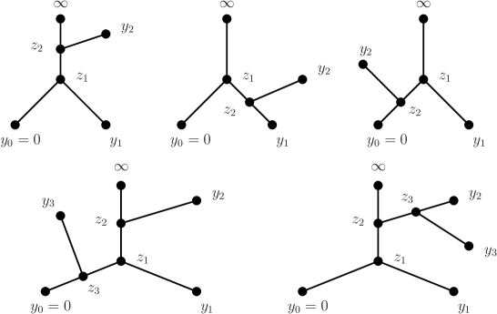
Figure 2: All three labelled tree graphs with $k=2$, and two of the five possible labelled tree graphs with $k=3$.

We can formalize the construction via the following recursive procedure. Let $\mathcal{T}(0)$ denote the set containing the unique tree with vertex set $\{0,\infty\}$. Assume that the collection $\mathcal{T}(k-1)$ of trees with vertex set $\{0,\dots,k-1\}\cup\{\infty\}\cup\{\bar{1},\dots,\overline{k-1}\}$ has been defined for some $k\geq 1$. Let $\mathcal{T}(k)$ denote the collection of trees with vertex set $\{0,\dots,k\}\cup\{\infty\}\cup\{\bar{1},\dots,\bar{k}\}$ that can be obtained in the following way. Pick some $\tau^{\prime}\in\mathcal{T}(k-1)$, and pick one of the edges of $\tau^{\prime}$. Split this edge into two by introducing a new vertex $\bar{k}$ on the edge, and add the new edge $\{k,\bar{k}\}$ to $\tau^{\prime}$. It is easy to see that any $\tau\in\mathcal{T}(k)$ has the following properties (see Figure 2):

• $\deg_{\tau}(\infty)=1=\deg_{\tau}(y_{i})$, $i=0,\dots,k$.

• $\deg_{\tau}(\bar{i})=3$, $i=1,\dots,k$.

With the above definitions, the event $\{y_{1},\dots,y_{k}\in{\mathcal{U}}_{0}\}$ implies that there exist $z_{1},\dots,z_{k}\in T(y_{0},\dots,y_{k},\infty)$ and $\tau\in\mathcal{T}(k)$ such that $T(y_{0},\dots,y_{k},\infty)$ is the edge-disjoint union of paths $T(\varphi(r),\varphi(s))$, where $\{r,s\}\in E(\tau)$, and $\varphi:V(\tau)\rightarrow\mathbb{Z}^{d}\cup\{\infty\}$ is defined by

$$\begin{cases}\varphi(i)=y_{i}&i=0,\dots,k;\\ \varphi(\infty)=\infty;\\ \varphi(\bar{i})=z_{i}&i=1,\dots,k.\end{cases}$$ (4.4)

Note that the choice of $\tau$ is not unique, due to possible coincidences between the vertices $y_{0},\dots,y_{k},z_{1},\dots,z_{k}$. We neglect the overcounting resulting from this, for an upper bound.

If the additional restriction $d_{\mathcal{U}}(0,y_{i})\leq n$, $i=1,\dots,k$ is in place, we must also have $d_{\mathcal{U}}(\varphi(r),\varphi(s))\leq n$ for all $\{r,s\}\in E(\tau)$ such that $r,s\not=\infty$. We define the event

$$\begin{split}&E(y_{1},\dots,y_{k},z_{1},\dots,z_{k},\tau,n)\\ &\qquad=\left\{\parbox{241.84842pt}{$T(y_{0},\dots,y_{k},\infty)=\cup_{\{r,s\}\in E(\tau)}T(\varphi(r),\varphi(s))$ as an edge-disjoint union and $d_{\mathcal{U}}(\varphi(r),\varphi(s))\leq n$ for all $\{r,s\}\in E(\tau)$ such that $r,s\not=\infty$}\right\}.\end{split}$$

Considering all possible choices of $\tau$ and $z_{1},\dots,z_{k}$, we get

$$\begin{split}{\mathbb{E}}\big{(}|B_{\mathcal{U}}(0,n)|^{k}\big{)}&=\sum_{y_{1},\dots,y_{k}\in\mathbb{Z}^{d}}{\mathbb{P}}\big{(}y_{1},\dots,y_{k}\in B_{\mathcal{U}}(0,n)\big{)}\\ &\leq\sum_{\tau\in\mathcal{T}(k)}\sum_{y_{1},\dots,y_{k}\in\mathbb{Z}^{d}}\sum_{z_{1},\dots,z_{k}\in\mathbb{Z}^{d}}{\mathbb{P}}\big{(}E(y_{1},\dots,y_{k},z_{1},\dots,z_{k},\tau,n)\big{)}.\end{split}$$

We use Wilson’s algorithm [W, LP] to replace the complicated event $E(y_{1},\dots)$ by a slightly larger event that is easier to handle. For this, enumerate the edges of $\tau$ as

$$\{r_{0},s_{0}\},\{r_{1},s_{1}\},\dots,\{r_{2k},s_{2k}\},$$

where the labelling is chosen in such a way that the following two properties are satisfied (see Figure 3(a)):

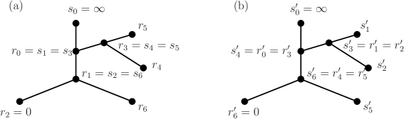
Figure 3: (a) A possible enumeration of edges for the application of Wilson’s method. (b) A possible enumeration of edges for performing the summations using (4.8) in the order $j=1,2,\dots,2k$. Summing over the spatial location $\varphi(s^{\prime}_{1})$ eliminates the factor involving the edge $\{s^{\prime}_{1},r^{\prime}_{1}\}$. Following this, it is possible to sum over $\varphi(s^{\prime}_{2})$, etc.

• $s_{0}=\infty$.

• For every $j=1,\dots,2k$, the set of edges $\{\{r_{\ell},s_{\ell}\}:\ell=0,\dots,j-1\}$ spans a subtree of $\tau$, and $s_{j}$ is a vertex of this subtree.

Using Wilson’s method with random walks started at $\varphi(r_{0}),\dots,\varphi(r_{2k})$, we see that

$$E(y_{1},\dots,y_{k},z_{1},\dots,z_{k},\tau,n)\subset\bigcap_{j=1}^{2k}F(\varphi(s_{j}),\varphi(r_{j}),n).$$ (4.5)

Here $F(\cdot,\cdot,n)$ are the events defined in (3.24). Importantly, the events on the right hand side are independent. Theorem 3.12 and the inclusion (4.5) imply that

$$\begin{split}&{\mathbb{P}}\big{(}E(y_{1},\dots,y_{k},z_{1},\dots,z_{k},\tau,n)\big{)}\\ &\qquad\leq\prod_{j=1}^{2k}C(1+|\varphi(s_{j})-\varphi(r_{j})|)^{2-d}\exp\left[-c\frac{|\varphi(s_{j})-\varphi(r_{j})|^{2}}{n}\right].\end{split}$$ (4.6)

It remains to estimate the sum of the right hand side of (LABEL:e:E-bnd) over all choices of the $y_{i}$’s and $z_{i}$’s. For this it will be convenient to use a different enumeration of $E(\tau)$. Suppose that

$$\{r^{\prime}_{0},s^{\prime}_{0}\},\{r^{\prime}_{1},s^{\prime}_{1}\},\dots,\{r^{\prime}_{2k},s^{\prime}_{2k}\}$$

satisfies the following properties (see Figure 3(b)).

• $s^{\prime}_{0}=\infty$ and $r^{\prime}_{2k}=0$.

• For every $j=1,\dots,2k$ the set $\{\{r^{\prime}_{\ell},s^{\prime}_{\ell}\}:\ell=j,\dots,2k\}$ induces a connected subtree of $\tau$, and $s^{\prime}_{j}$ is a leaf of this subtree.

For ease of notation, let us write $u_{j}=\varphi(r^{\prime}_{j})$ and $w_{j}=\varphi(s^{\prime}_{j})$. With the new enumeration the right hand side of (LABEL:e:E-bnd) takes the following form:

$$\begin{split}&{\mathbb{P}}\big{(}E(y_{1},\dots,y_{k},z_{1},\dots,z_{k},\tau,n)\big{)}\\ &\qquad\leq\prod_{j=1}^{2k}C(1+|w_{j}-u_{j}|)^{2-d}\exp\left[-c\frac{|w_{j}-u_{j}|^{2}}{n}\right].\end{split}$$ (4.7)

Note again that the $w_{j}$’s and $u_{j}$’s are $z_{i}$’s and $y_{i}$’s, determined implicitly by $\tau$. Importantly, property (b’) of the enumeration implies that if $w_{j}=\varphi(s^{\prime}_{j})=z_{i}$ for some $i,j$, then the variable $z_{i}$ does not occur in the product

$$\prod_{\ell=j+1}^{2k}C(1+|w_{j}-u_{j}|)^{2-d}\exp\left[-c\frac{|w_{j}-u_{j}|^{2}}{n}\right].$$

Similar considerations apply if $w_{j}=\varphi(s^{\prime}_{j})=y_{i}$ for some $i,j$. The summation over $y_{1},\dots,y_{k}$ and $z_{1},\dots,z_{k}$ can be accomplished by the following lemma.

Lemma 4.2.

For any $u\in\mathbb{Z}^{d}$, we have

$$\sum_{w\in\mathbb{Z}^{d}}(1+|w-u|)^{2-d}\exp\left[-c\frac{|w-u|^{2}}{n}\right]\leq Cn.$$ (4.8)

We apply Lemma 4.2 successively to the factors with $j=1,\dots,2k$ on the right hand side of (LABEL:e:E-bnd2). See Figure 3(b) for an example of how the edges of $\tau$ are successively removed by the summations. We obtain

$${\mathbb{E}}\big{(}|B_{\mathcal{U}}(0,n)|^{k}\big{)}\leq\sum_{\tau\in\mathcal{T}(k)}(Cn)^{2k}.$$ (4.9)

Since the number of trees in $\mathcal{T}(k)$ is $1\cdot 3\cdot\cdots(2k-1)\leq 2^{k}k!$, this proves (4.2). $\square$

Remark 4.3.

The statements of Theorem 4.1 still hold, with essentially the same proof, when ${\mathcal{U}}={\mathcal{U}}_{D}$, with any $D\subset{\mathbb{Z}}^{d}$. Note that ${\mathcal{U}}_{0}$ still has one end. This follows from [LMS, Proposition 3.1], and the fact that the component of $0$ under the measure $\mathsf{WSF}_{o}$ in the domain $D$ is stochastically smaller then it is in ${\mathbb{Z}}^{d}$. Therefore, a decomposition into events $E(y_{1},\dots,y_{k},z_{1},\dots,z_{k},n)$ still holds (with ${\mathcal{U}}={\mathcal{U}}_{D}$), where now all vertices are in $D$. The inclusion (4.5) still holds, with the events $F$ having the same meaning as before. This allows to bound the summations in exactly the same way as in ${\mathbb{Z}}^{d}$.

5 Lower bounds on volumes

In this section we return to the setup of Section 3, in order to give a lower bound on the volume of ${\mathcal{U}}_{0}$. We first estimate the number of vertices of ${\mathcal{U}}_{0}$ in shells $Q_{n+m}\setminus Q_{n}$. Recall that $Q_{N}\subset D\subset{\mathbb{Z}}^{d}$, and $n,m$ satisfy $16\leq n<n+m\leq N$, with $m\leq n/8$. We have $L={\mathcal{L}}({\mathcal{E}}^{F}_{D^{c}}(S))$, $\alpha={\mathcal{E}}^{F}_{\partial_{i}Q_{n}}L$, and $x_{0}\in\partial_{i}Q_{n}$ is the endpoint of $\alpha$. The remaining piece of $L$ is $L^{\prime}={\mathcal{B}}^{F}_{\partial_{i}Q_{n}}L$, and $\beta={\mathcal{E}}^{F}_{\partial_{i}Q(x_{0},m)}L^{\prime}$. See Figure 4.

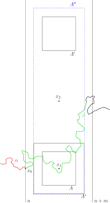
Figure 4: Boxes for the cycle popping argument.

Recall that when $x_{0}\in{\mathbb{H}}_{n}$, we defined $A=A(x_{0})=Q(x_{0}+(m/2)e_{1},m/4)$ and $x_{1}=x_{0}+(m/2)e_{1}$, with appropriate rotations applied when $x_{0}$ was on a different face of $Q_{n}$. We will now also need a point $x_{2}\in Q_{n+m}\setminus Q_{n}$ of order $m$ away from $A$, and further boxes contained in $Q_{n+m}\setminus Q_{n}$ that we define as follows. If $x_{0}\in{\mathbb{H}}_{n}$ and the second coordinate of $x_{0}$ is negative, let

$$\begin{split}x_{2}&=x_{1}+me_{2}\\ A^{\prime}&=A^{\prime}(x_{0})=Q(x_{1}+2me_{2},m/4)\\ A^{\prime\prime}&=A^{\prime\prime}(x_{0})=x_{1}+[-3m/8,3m/8]\times[-m,3m]\times[-m,m]^{d-2}\cap{\mathbb{Z}}^{d}.\end{split}$$ (5.1)

If $x_{0}\in{\mathbb{H}}_{n}$ and the second coordinate of $x_{0}$ is positive, we replace $e_{2}$ by $-e_{2}$ and $[-m,3m]$ by $[-3m,m]$. If $x_{0}$ is on a different face of $Q_{n}$, we replace $e_{1}$ and $e_{2}$ by two other suitable unitvectors.

The key technical estimate is to show that $\beta\cap A$ has capacity of order $m^{2}$ with probability bounded away from $0$, which we do in the next section.

5.1 A capacity estimate

Let $S^{x_{2}}$ be a random walk with $S^{x_{2}}(0)=x_{2}$, independent of $S$, $\tilde{X}$, etc.

Proposition 5.1.

Assume $N\geq 1$, $Q_{4N}\subset D\subset{\mathbb{Z}}^{d}$, and the setup of Section 3.
(a) There exists $c_{1}=c_{1}(d)>0$ such that

$${\mathbb{P}}\big{(}\text{$S^{x_{2}}$ hits $(A\cap\beta)$}\,\big{|}\,\alpha\big{)}\geq c_{1}m^{4-d}.$$

(b) We have

$${\mathbb{P}}\big{(}cm^{2}\leq\mathrm{Cap}(A\cap\beta)\leq C_{1}m^{2}\,\big{|}\,\alpha\big{)}\geq c>0.$$ (5.2)

Proof. (a) For ease of notation, we omit the conditioning on $\alpha$. Let

$$U:=\sum_{z\in A}I[z\in\beta]I[\text{$S^{x_{2}}$ hits $z$}],$$

so that

$${\mathbb{P}}\big{(}\text{$S^{x_{2}}$ hits $(A\cap\beta)$}\big{)}={\mathbb{P}}(U>0).$$

Using Lemma 3.9, we have

$$\begin{split}{\mathbb{E}}(U)=\sum_{z\in A}{\mathbb{P}}(z\in\beta){\mathbb{P}}\big{(}T_{z}[S^{x_{2}}]<\infty\big{)}\geq cm^{d}m^{2-d}m^{2-d}=cm^{4-d}.\end{split}$$

On the other hand,

$${\mathbb{E}}\big{(}U^{2}\big{)}=\sum_{x,y\in A}{\mathbb{P}}(x,y\in\beta)\,{\mathbb{P}}\big{(}T_{x}[S^{x_{2}}]<\infty,\,T_{y}[S^{x_{2}}]<\infty\big{)}.$$ (5.3)

Since the process $\widetilde{X}$ generating $L^{\prime}$ must pass through $\partial A^{*}$ in order for the event $x,y\in\beta$ to occur, we have

$$\begin{split}{\mathbb{P}}(x,y\in\beta)&\leq\max_{z\in\partial A^{*}}[\widetilde{G}_{D}(z,x)\widetilde{G}_{D}(x,y)+\widetilde{G}_{D}(z,y)\widetilde{G}_{D}(y,x)]\\ &\leq Cm^{2-d}G(x,y).\end{split}$$

For the other term in the right hand side of (5.3) we have

$$\begin{split}{\mathbb{P}}\big{(}T_{x}[S^{x_{2}}]<\infty,\,T_{y}[S^{x_{2}}]<\infty\big{)}&\leq[G(x_{2},x)G(x,y)+G(x_{2},y)G(y,x)]\\ &\leq Cm^{2-d}G(x,y).\end{split}$$

Since $d\geq 5$, we have $\sum_{x,y\in A}G(x,y)^{2}\leq Cm^{d}$, which gives ${\mathbb{E}}\big{(}U^{2}\big{)}\leq Cm^{4-d}$.

The Paley-Zygmund inequality then gives

$${\mathbb{P}}\big{(}\text{$S^{x_{2}}$ hits $(A\cap\beta)$}\big{)}={\mathbb{P}}(U>0)\geq\frac{{\mathbb{E}}(U)^{2}}{{\mathbb{E}}\big{(}U^{2}\big{)}}\geq cm^{4-d}.$$

(b) Since $\mathrm{Cap}(A\cap\beta)\leq C|A\cap\beta|$, and $m^{2-d}\mathrm{Cap}(A\cap\beta)\asymp{\mathbb{P}}\big{(}T_{A\cap\beta}[S^{x_{2}}]<\infty\,\big{|}\,\beta\big{)}$, combining (a) with Lemma 3.3 gives (b). $\square$

Assume now, similarly to Proposition 3.11, that $k\geq 1$ and $m\geq 4$ such that $N/2\leq km<N-m$. Recall that for $j=1,\dots,k$ we denote $\alpha_{j}={\mathcal{E}}^{F}_{\partial_{i}Q(0,jm)}L$. Let $Y_{j}=\alpha_{j}(|\alpha_{j}|)$ be the last point in $\alpha_{j}$, and $\beta_{j}={\mathcal{E}}^{F}_{\partial_{i}Q(Y_{j},m)}({\mathcal{B}}^{F}_{\partial_{i}Q(0,jm)}L)$ be the path $L$ between $Y_{j}$ and its first hit after $Y_{j}$ on $\partial_{i}(Y_{j},m)$. Let $Y_{j,1}$ and $Y_{j,2}$ be the points $x_{1}$ and $x_{2}$ defined with respect to $x_{0}=Y_{j}$, respectively. Define the following event, measurable with respect to $L$:

$$G(c_{1},c_{2},C_{1})=\left\{\parbox{256.0748pt}{there are at least $c_{2}k$ indices $j$ with $1\leq j\leq k$ such that ${\mathbb{P}}\big{(}T_{A(Y_{j})\cap\beta_{j}}[S^{Y_{j,2}}]<\infty\,\big{|}\,L\big{)}\geq c_{1}m^{4-d}$ and $|Q(Y_{j},m)\cap\beta_{j}|\leq C_{2}m^{2}$}\right\}.$$ (5.4)

Proposition 5.1 and an argument similar to that of Proposition 3.11 gives the following corollary.

Corollary 5.2.

Under the assumptions of Proposition 5.1, there exist $c_{1},c_{2}>0$ and $C_{2}$ such that we have

$$\begin{split}{\mathbb{P}}\left[G(c_{1},c_{2},C_{2})\right]\geq 1-\exp(-ck).\end{split}$$ (5.5)

Remark 5.3.

We note the following minor extension of Corollary 5.2. Assuming still that $Q_{4N}\subset D$, let $w\in\partial D$ be fixed, condition $S$ to exit $D$ at $w$, and let $L^{\prime}={\mathcal{L}}({\mathcal{E}}^{F}_{D^{c}}S)$ be the loop-erasure. Masson [Mas] proves that the law of ${\mathcal{E}}^{F}_{Q_{N}^{c}}L^{\prime}$ is comparable, up to constants factors, to the law of ${\mathcal{E}}^{F}_{Q_{N}^{c}}L$. Since the event $G(c_{1},c_{2},C_{2})$ is measurable with respect to ${\mathcal{E}}^{F}_{Q_{N}^{c}}L$, the statement of the corollary follows also for $L^{\prime}$.

5.2 Lower bound on $|Q_{N}\cap{\mathcal{U}}_{0}|$

We continue with the setup of the previous section. Our argument will use the cycle popping idea of Wilson [W]; see also [LP].

Theorem 5.4.

Assume $N\geq 1$, $Q_{4N}\subset D\subset{\mathbb{Z}}^{d}$, and let ${\mathcal{U}}={\mathcal{U}}_{D}$. There exist constants $C,c$, such that

$${\mathbb{P}}\big{(}|Q_{N}\cap{\mathcal{U}}_{0}|\leq\lambda N^{4}\big{)}\leq C\exp(-c\lambda^{-1/3}).$$

Proof. Condition on $L$, and assume that the event (5.4) occurs. Let $J$ be the set of indices $1\leq j\leq k$ (a $\sigma(L)$-measurable random set) satisfying the requirements in this event. For each $j\in J$, let

$$A^{\prime}(j)=A^{\prime}(Y_{j})\qquad A^{\prime\prime}(j)=A^{\prime\prime}(Y_{j}).$$

The definitions of $A^{\prime}$ and $A^{\prime\prime}$ made in (5.1) ensure that $A^{\prime\prime}(j)$, $j\in J$ are disjoint.

We will need two coupled collections of stacks. Associate to each $z\in(\cup_{j\in J}A^{\prime\prime}(j))\setminus L$ a stack of arrows, and let us call these $\mathsf{Stacks\ I}$. For each $j\in J$ and each $z\in A^{\prime\prime}(j)\cap L\setminus\beta_{j}$, pick a new independent stack leaving the rest of the stacks unchanged. Call this second collection of stacks $\mathsf{Stacks\ II}$. In both $\mathsf{Stacks\ I}$ and $\mathsf{Stacks\ II}$, and for every $j\in J$, pop all cycles that are entirely contained in $A^{\prime\prime}(j)$. That is, if a cycle starts in $A^{\prime\prime}(j)$, but part of it lies outside $A^{\prime\prime}(j)$, we do not pop it. It is important to note that the order of popping cycles is irrelevant for determining the final configuration on the top of the stacks.

For each $j\in J$, let

$$\begin{split}V^{I}_{j}&=\left\{y\in A^{\prime}(j):\parbox{156.49014pt}{cycle popping using $\mathsf{Stacks\ I}$ reveals a path from $y$ to $L$}\right\}\\ V^{II}_{j}&=\left\{y\in A^{\prime}(j):\parbox{179.25244pt}{cycle popping using $\mathsf{Stacks\ II}$ \\ reveals a path from $y$ to $A^{\prime\prime}(j)\cap\beta_{j}$}\right\}\end{split}$$

Note that $(V^{I}_{j},V^{II}_{j})_{j\in J}$ are conditionally independent, given $L$, $J$.

Lemma 5.5.

We have $V^{I}_{j}\supset V^{II}_{j}$ for all $j\in J$.

Proof. Let $y\in V^{II}_{j}$, and consider $\mathsf{Stacks\ II}$. Starting from $y$, follow the arrows in $\mathsf{Stacks\ II}$, until $A^{\prime\prime}(j)\cap\beta_{j}$ is hit. Removing cycles chronologically from this path pops some cycles entirely contained in $A^{\prime\prime}(j)$, and reveals a path from $y$ to $A^{\prime\prime}(j)\cap\beta_{j}$. Now if we follow the arrows in $\mathsf{Stacks\ I}$ instead, then the same arrows are used until the first time $L$ is hit. This guarantees that a path from $y$ to $L$ is revealed, that does not leave $A^{\prime\prime}(j)$, and hence $y\in V^{I}_{j}$.

Lemma 5.6.

Assume $d\geq 5$. For some $c_{3}>0$ we have

$${\mathbb{P}}\big{(}|V^{II}_{j}|\geq c_{3}m^{4}\,\big{|}\,L,\,j\in J\big{)}\geq c>0.$$

Proof. We estimate the first and second moments of $|V^{II}_{j}|$.

Fix $y\in A^{\prime}(j)$. Following the arrows from $y$ in $\mathsf{Stacks\ II}$ we perform a random walk until either we exit $A^{\prime\prime}(j)$, or we hit $A^{\prime\prime}(j)\cap\beta_{j}$. Therefore,

$$\begin{split}{\mathbb{P}}\big{(}y\in V^{II}_{j}\,\big{|}\,L,\,j\in J\big{)}&={\mathbb{P}}\big{(}T_{A^{\prime\prime}(j)\cap\beta_{j}}[S^{y}]<\tau_{A^{\prime\prime}(j)}[S^{y}]\,\big{|}\,L,\,j\in J\big{)}\\ &\geq{\mathbb{P}}\big{(}T_{A(j)\cap\beta_{j}}[S^{y}]<\tau_{A^{\prime\prime}(j)}[S^{y}]\,\big{|}\,L,\,j\in J\big{)}.\end{split}$$ (5.6)

The last expression is

$$\geq c{\mathbb{P}}\big{(}T_{A(j)\cap\beta_{j}}[S^{y}]<\infty\,\big{|}\,L,\,j\in J\big{)}.$$ (5.7)

(One way to see this is by an argument similar to that of Lemma 3.6, where we let $R$ count the number of crossings by the walk from a box $A^{**}\subset A^{\prime\prime}(j)$ to $\partial A^{\prime\prime}(j)$ before hitting $\beta_{j}\cap A(j)$, where each face of $\partial A^{**}$ is at distance $m/16$ away from the corresponding face of $\partial A^{\prime\prime}(j)$.)

The Harnack inequality and Proposition 5.1 now implies, after summing over $y$ in (5.6)–(5.7), that

$${\mathbb{E}}\big{(}|V^{II}_{j}|\,\big{|}\,L,\,j\in J\big{)}\geq cc_{1}m^{d}m^{4-d}=cm^{4}.$$

We now bound the second moment of $|V^{II}_{j}|$. If $x,y\in V^{II}_{j}$ occurs, then there exists a unique $w\in A^{\prime\prime}(j)$ with the property that cycle popping reveals three edge-disjoint paths: one from $w$ to $A^{\prime\prime}(j)\cap\beta_{j}$, a second from $x$ to $w$ and a third from $y$ to $w$. (We allow to have $x=w$ or $y=w$ or both.) When this event happens with a fixed $w$, we can reveal the paths by first following the arrows starting from $w$ until $A^{\prime\prime}(j)\cap\beta_{j}$ is hit, then following the arrows starting from $x$ until $w$ is hit, then following the arrows starting from $y$ until $w$ is hit. This shows that

$$\begin{split}&{\mathbb{P}}\big{(}x,y\in V^{II}_{j}\,\big{|}\,L,\,j\in J\big{)}\\ &\qquad\leq\sum_{w\in A^{\prime\prime}(j)}{\mathbb{P}}\big{(}T_{A^{\prime\prime}(j)\cap\beta_{j}}[S^{w}]<\infty\,\big{|}\,L,\,j\in J\big{)}\,{\mathbb{P}}\big{(}T_{w}[S^{x}]<\infty\big{)}\,{\mathbb{P}}\big{(}T_{w}[S^{y}]<\infty\big{)}.\end{split}$$ (5.8)

Let $\tilde{A}(j)=Q(Y_{j,1},(3m/2))$, and note that $\partial\tilde{A}(j)$ has distance at least $cm$ from $A^{\prime\prime}(j)\cap\beta_{j}$, and also distance at least $cm$ from $A^{\prime}(j)$. We estimate separately the cases:
(a) $w\in A^{\prime\prime}(j)\setminus\tilde{A}(j)$; and
(b) $w\in A^{\prime\prime}(j)\cap\tilde{A}(j)$.
The sum of the terms in the right hand side of (LABEL:e:VII2ndm-ub) corresponding to case (a) is at most:

$$\begin{split}&Cm^{2-d}\mathrm{Cap}(A^{\prime\prime}(j)\cap\beta_{j})\sum_{w\in A^{\prime\prime}(j)\setminus\tilde{A}(j)}\sum_{x,y\in A^{\prime}(j)}G(x,w)G(y,w)\\ &\qquad\leq Cm^{2-d}m^{2}m^{2}m^{2}m^{d}=Cm^{8}.\end{split}$$

The sum for case (b) is at most:

$$\begin{split}&Cm^{2-d}m^{2-d}m^{d}m^{d}\sum_{w\in A^{\prime\prime}(j)\cap\tilde{A}(j)}{\mathbb{P}}\big{(}T_{A^{\prime\prime}(j)\cap\beta_{j}}[S^{w}]<\infty\big{)}\\ &\qquad\leq Cm^{4}\sum_{w\in\tilde{A}(j)}{\mathbb{P}}\big{(}T_{A^{\prime\prime}(j)\cap\beta_{j}}[S^{w}]<\tau_{\tilde{A}(j)}\big{)}\\ &\qquad\leq Cm^{4}m^{2}\mathrm{Cap}(A^{\prime\prime}(j)\cap\beta_{j})\\ &\qquad\leq Cm^{8}.\end{split}$$

Here the last line follows from $j\in J$ and Proposition 5.1.

The moment estimates for $|V^{II}_{j}|$ and the one-sided Chebyshev inequality yield:

$${\mathbb{P}}\big{(}V^{II}_{j}\geq cm^{4}\,\big{|}\,L,\,j\in J\big{)}\geq c>0.$$

This completes the proof of the Lemma.

We can now complete the proof of Theorem 5.4. Choose $k\asymp\lambda^{-1/3}$ so that $\lambda N^{4}\asymp km^{4}$. Then using Corollary 5.2, the conditional independence of $(V^{II}_{j})_{j\in J}$, and Lemma 5.5, for a suitably small $c_{4}>0$ we have

$$\begin{split}{\mathbb{P}}\big{(}|Q_{N}\cap{\mathcal{U}}_{0}|\leq\lambda N^{4}\big{)}&\leq C\exp(-ck)+{\mathbb{E}}\bigg{(}{\mathbb{P}}\bigg{(}\parbox{113.81102pt}{$V^{II}_{j}\geq c_{3}m^{4}$ for less than $c_{4}k$ indices $j\in J$}\,\bigg{|}\,L\bigg{)}I[G(c_{1},c_{2},C_{2})]\bigg{)}\\ &\leq C\exp(-c\lambda^{-1/3}).\end{split}$$

This completes the proof of the Theorem.

Theorem 5.7.

Assume $d\geq 5$ and let ${\mathcal{U}}={\mathcal{U}}_{{\mathbb{Z}}^{d}}$. There exist $c>0$ and $C$ such that for all $\lambda>0$ we have

$${\mathbb{P}}\big{(}|B_{\mathcal{U}}(0,n)|\leq\lambda n^{2}\big{)}\leq C\exp(-c\lambda^{-1/5}).$$

For the proof of this theorem, we assume the setting of Proposition 3.11, with $D=\mathbb{Z}^{d}$. Recall that $M_{N}=|{\mathcal{E}}^{F}_{\partial_{i}Q_{N}}L|$.

Lemma 5.8.

We have

$${\mathbb{E}}\big{(}M_{N}^{k}\big{)}\leq C_{2}^{k}k!N^{2k}.$$

Consequently, there exist $c>0$ and $C$ such that for all $\lambda>0$ we have

$${{\mathbb{P}}\big{(}M_{N}\geq\lambda N^{2}\big{)}\leq C\exp(-c\lambda).}$$ (5.9)

Remark 5.9.

If $M^{S}_{N}$ is the length of a simple random walk path run until its first exit from $Q_{N}$ then it is well known that $M^{S}_{N}/N^{2}$ has an exponential tail. However we do not have $M_{N}\leq M^{S}_{N}$, so need an alternative argument to obtain the bound (5.9).

Proof. [Proof of Lemma 5.8.] We have

$$\begin{split}{\mathbb{E}}\big{(}M_{N}^{k}\big{)}&\leq{\mathbb{E}}\big{(}|S[0,\infty)\cap Q_{N}|^{k}\big{)}\\ &=k!\sum_{x_{1},\dots,x_{k}\in Q_{N}}G(0,x_{1})G(x_{1},x_{2})\dots G(x_{k-1},x_{k})\\ &\leq k!\Big{(}\sum_{z\in Q_{2N}}G(0,z)\Big{)}^{k}\\ &=C_{2}^{k}k!N^{2k}.\end{split}$$

To see the second statement:

$${\mathbb{P}}\big{(}M_{N}\geq\lambda N^{2}\big{)}\leq\exp(-\lambda tN^{2}){\mathbb{E}}\big{(}e^{tM_{N}}\big{)}\leq\exp(-\lambda tN^{2})\frac{1}{1-C_{2}tN^{2}}.$$

Choosing $t=1/(2C_{2}N^{2})$ completes the proof of the Lemma.

Proof. [Proof of Theorem 5.7] It is sufficient to prove the statement for $0<\lambda<\lambda_{0}$ for some fixed $\lambda_{0}$. Let us choose $N=\lambda^{\alpha}\sqrt{n}$ with some exponent $\alpha>0$, that we will optimize over at the end of the proof. We have

$${\mathbb{P}}(M_{N}\geq n/2)\leq C\exp\Big{(}-c\frac{n}{2N^{2}}\Big{)}=C\exp(-c\lambda^{-2\alpha}).$$

Condition on $L$, as in the proof of Theorem 5.4, and assume the event

$$\widetilde{G}=G(c_{1},c_{2},C_{1})\cap\{M_{N}<n/2\}.$$

We set

$$\lambda n^{2}=c_{3}km^{4}\asymp Nm^{3},$$

which means we pick $m$ to be

$$m\asymp\sqrt{n}\lambda^{(1-\alpha)/3}.$$

Hence $N/m\asymp k\asymp\lambda^{(4\alpha-1)/3}$. Note that this implies that

$${\mathbb{P}}\big{(}G(c_{1},c_{2},C_{1})^{c}\big{)}\leq C\exp(-c(N/m))=C\exp(-c\lambda^{(4\alpha-1)/3}).$$

Since we want $N/m\gg 1$, we impose the condition $0<\alpha<1/4$ on $\alpha$.

For each $j\in J$, let

$$\begin{split}\widetilde{V}^{I}_{j}&=\left\{y\in A^{\prime}(j):\parbox{227.62204pt}{cycle popping using $\mathsf{Stacks\ I}$ reveals a path from $y$ to $L$ of lenght $\leq n/2$}\right\}\\ \widetilde{V}^{II}_{j}&=\left\{y\in A^{\prime}(j):\parbox{227.62204pt}{cycle popping using $\mathsf{Stacks\ II}$ reveals a path from $y$ to $A^{\prime\prime}(j)\cap\beta_{j}$ of length $\leq n/2$}\right\}\end{split}$$

Notice that $(\widetilde{V}^{I}_{j},\widetilde{V}^{II}_{j})_{j\in J}$ are again conditionally independent, given $L$. The same proof as in Lemma 5.5 shows that we have $\widetilde{V}^{I}_{j}\supset\widetilde{V}^{II}_{j}$ for all $j\in J$.

In estimating ${\mathbb{E}}\big{(}\widetilde{V}^{II}\big{)}$ from below, we write

$$\begin{split}{\mathbb{P}}\big{(}y\in\widetilde{V}^{II}_{j}\,\big{|}\,L,\,j\in J\big{)}&\geq{\mathbb{P}}\big{(}T_{A^{\prime\prime}(j)\cap\beta_{j}}[S^{y}]<\tau_{A^{\prime\prime}(j)}[S^{y}]\,\big{|}\,L,\,j\in J\big{)}\\ &\qquad-{\mathbb{P}}\big{(}|{\mathcal{E}}^{F}_{\partial A^{\prime\prime}(j)}(S^{y})|>n/2,\,T_{A^{\prime\prime}(j)\cap\beta_{j}}[S^{y}]\circ\Theta_{n/2}<\infty\big{)}.\end{split}$$ (5.10)

The first term on the right hand side is $\geq cm^{4-d}$ due to (5.7) and $j\in J$. We now show that the subtracted term is $\leq C\exp(-cn/m^{2})m^{4-d}$.

Note that we may restrict to $n/2>2m^{2}$ for convenience (although not needed for the claim), since our choice of $m$ implies that $n\asymp m^{2}\lambda^{-2(1-\alpha)/3}$, and we are considering small $\lambda$. Using the Markov property at time $n/2-m^{2}$, the second term in the right hand side of (5.10) is at most

$${\mathbb{P}}^{y}\big{(}\tau_{A^{\prime\prime}(j)}>n/2-m^{2}\big{)}\,\sum_{z\in A^{\prime\prime}(j)}{\mathbb{P}}^{z}\big{(}T_{A^{\prime\prime}(j)\cap\beta_{j}}<\infty\big{)}\,{\mathbb{P}}^{y}\big{(}S(n/2)=z\,\big{|}\,\tau_{A^{\prime\prime}(j)}>n/2-m^{2}).$$

The first probability can be bounded by $C\exp(-cn/m^{2})$, by considering stretches of the walk of length $m^{2}$, in each of which there is probability $\geq c>0$ of exit from $A^{\prime\prime}(j)$. The conditional distribution of $z$ is bounded above by $cm^{-d}$, due to the local CLT applied to $S(n/2-m^{2}),\dots,S(n/2)$. Hence we are left to show that

$$\sum_{z\in A^{\prime\prime}(j)}{\mathbb{P}}^{z}\big{(}T_{A^{\prime\prime}(j)\cap\beta_{j}}<\infty\big{)}\leq m^{4}.$$

Let us write $\widetilde{\beta}_{j}=A^{\prime\prime}(j)\cap\beta_{j}$, and $h(z)={\mathbb{P}}^{z}(T_{\widetilde{\beta}_{j}}<\infty)$. By a last exit decomposition $h(z)=\sum_{u\in\widetilde{\beta}_{j}}G(z,u)e_{\widetilde{\beta}_{j}}(u)$, where $e_{\widetilde{\beta}_{j}}(u)={\mathbb{P}}^{u}(T^{+}_{\widetilde{\beta}_{j}}=\infty)$. Therefore, we have

$$\begin{split}\sum_{z\in A^{\prime\prime}(j)}h(z)&=|\widetilde{\beta}_{j}|+\sum_{z\in A^{\prime\prime}(j)\setminus\widetilde{\beta}_{j}}h(z)\leq Cm^{2}+\sum_{u\in\widetilde{\beta}_{j}}\sum_{z\in A^{\prime\prime}(j)}G(z,u)e_{\widetilde{\beta}_{j}}(u)\\ &\leq Cm^{2}+Cm^{2}\sum_{u\in\widetilde{\beta}_{j}}e_{\widetilde{\beta}_{j}}(u)=Cm^{2}+Cm^{2}\mathop{{\rm Cap}}(\widetilde{\beta}_{j})\leq Cm^{4},\end{split}$$

using that $|\widetilde{\beta}_{j}|,\mathop{{\rm Cap}}(\widetilde{\beta}_{j})\leq Cm^{2}$ when $j\in J$.

Hence we obtain that there exists $\lambda_{0}=\lambda_{0}(d)>0$, such that when $0<\lambda\leq\lambda_{0}$, the right hand side of (5.10) is at least

$$\begin{split}cm^{4-d}-C\,\exp(-cn/m^{2})\,m^{4-d}\geq cm^{4-d}-C\,\exp(-c\lambda^{-2(1-\alpha)/3})\,m^{4-d}\geq cm^{4-d}.\end{split}$$

It follows that ${\mathbb{E}}\big{(}|\widetilde{V}^{II}_{j}|\,\big{|}\,L,\,j\in J\big{)}\geq cm^{4}$.

For the second moment, we simply estimate

$${\mathbb{E}}\big{(}(\widetilde{V}^{II}_{j})^{2}\,\big{|}\,L,\,j\in J\big{)}\leq{\mathbb{E}}\big{(}(V^{II}_{j})^{2}\,\big{|}\,L,\,j\in J\big{)}\leq Cm^{8}.$$

The one-sided Chebyshev inequality yields that for some $c_{4}=c_{4}(d)>0$ we have

$${\mathbb{P}}\big{(}\widetilde{V}^{II}_{j}\geq c_{4}m^{4}\,\big{|}\,L,\,j\in J\big{)}\geq c>0.$$

This allows us to complete the proof as follows.

$$\begin{split}&{\mathbb{P}}\big{(}|B_{\mathcal{U}}(0,n)|\leq\lambda n^{2}\big{)}\\ &\qquad\leq{\mathbb{P}}\big{(}\widetilde{G}^{c}\big{)}+{\mathbb{P}}\Big{(}\widetilde{G},\,\sum_{j\in J}\widetilde{V}^{I}_{j}\leq\lambda n^{2}\Big{)}\\ &\qquad\leq{\mathbb{P}}(M_{N}>n/2)+{\mathbb{P}}\big{(}G(c_{1},c_{2},C_{1})^{c}\big{)}+{\mathbb{E}}\Big{(}{\mathbb{P}}\Big{(}\sum_{j\in J}\widetilde{V}^{II}_{j}<c_{3}km^{4}\,\Big{|}\,L\Big{)};\widetilde{G}\Big{)}\\ &\qquad\leq C\exp(-c\lambda^{-2\alpha})+C\exp(-c\lambda^{(4\alpha-1)/3})+\exp(-c\lambda^{(4\alpha-1)/3}).\end{split}$$

We choose $\alpha$, so that $-2\alpha=(4\alpha-1)/3$, so $\alpha=1/10$. This completes the proof of the Theorem.

Remark 5.10.

We note the following minor extension of Theorem 5.4, that is needed in [BHJ]. Similarly to Remark 5.3, since the arguments of Theorem 5.4 only rely on properties of ${\mathcal{E}}^{F}_{Q_{N}^{c}}L$, the result extends to the case when the component of the origin is connected to a fixed vertex $w\in\partial D$.

MB: Department of Mathematics, University of British Columbia, Vancouver, BC V6T 1Z2, Canada.
barlow@math.ubc.ca

AAJ: Department of Mathematical Sciences, University of Bath, Claverton Down, Bath BA2 7AY, United Kingdom.
A.Jarai@bath.ac.uk

References

[AN] M. Aizenman and C.M. Newman.
Tree graph inequalities and critical behavior in percolation models.
J. Stat. Phys.36 Nos. 1/2, (1984), 107–143.
[BK]
M.T. Barlow and D. Karlı.
Some remarks on uniform boundary Harnack Principles.
Preprint. (2015),
arxiv.org/abs/1507.04115
[BM1]
M.T. Barlow and R. Masson. Exponential tail bounds for loop-erased random walk
in two dimensions.
Ann. Probab.38 No. 6, (2010), 2379–2417.
[BM2]
M.T. Barlow and R. Masson.
Spectral dimension and random walks on the two dimensional uniform spanning tree.
Comm. Math. Phys.305 (2011), 23–57.
[BLPS]
I. Benjamini, R. Lyons, Y. Peres and O. Schramm.
Uniform spanning forests.
Ann. Probab.29 (2001), 1–65.
[BHJ]
S. Bhupatiraju, J. Hanson and A.A. Járai.
Inequalities for critical exponents in -dimensional sandpiles.
Preprint. (2016)
[La1]
G.F. Lawler.
A self-avoiding random walk.
Duke Math. J., 47(3):655–693, 1980.
[La2]
G.F. Lawler.
Intersections of random walks.
Probability and its Applications. Birkhäuser Boston Inc., Boston,
MA, 1991.
[La3]
G.F. Lawler.
The logarithmic correction for loop-erased walk in four dimensions.
In Proceedings of the Conference in Honor of Jean-Pierre Kahane
(Orsay, 1993), number Special Issue, pages 347–361, 1995.
[Law99]
G.F. Lawler.
Loop-erased random walk.
In: Perplexing problems in probability, ed. M. Bramson, R. Durrett.
(Progress in probability, vol. 44),
Birkhäuser, 1999.
[LMS]
R. Lyons, B.J. Morris and O. Schramm.
Ends in uniform spanning forests.
Electron. J. Probab.13 (2008), no. 58, 1702–1725.
[LP]
R. Lyons with Y. Peres.
Probability on Trees and Networks.
Cambridge University Press.
In preparation. Current
version available at http://pages.iu.edu/~rdlyons/.
[LL]
G.F. Lawler and V. Limic.
Random walk: a modern introduction, 2009.
Cambridge University Press.
[Mas]
R. Masson.
The growth exponent for planar loop-erased random walk.
Electron. J. Probab., 14 paper no. 36, 1012–1073, 2009.
[Pem91] R. Pemantle:
Choosing a spanning tree for the integer lattice uniformly.
Ann. Probab.19 (1991), no. 4, 1559–1574.
[W] D.B. Wilson.
Generating spanning trees more quickly than the cover time.
Proceedings of the Twenty-eighth Annual ACM Symposium on the
Theory of Computing (Philadelphia, PA, 1996), 296–303, ACM, New York, 1996.