Level-set methods for convex optimization

Abstract

Convex optimization problems arising in applications often have favorable objective functions and complicated constraints, thereby precluding first-order methods from being immediately applicable. We describe an approach that exchanges the roles of the objective and constraint functions, and instead approximately solves a sequence of parametric level-set problems. A zero-finding procedure, based on inexact function evaluations and possibly inexact derivative information, leads to an efficient solution scheme for the original problem. We describe the theoretical and practical properties of this approach for a broad range of problems, including low-rank semidefinite optimization, sparse optimization, and generalized linear models for inference.

1 Introduction

To motivate the discussion, consider the typical problem of recovering a sparse vector $x$ that approximately satisfies the linear system $Ax=b$. This task often arises in applications, such as compressed sensing and model selection. Standard approaches, based on convex optimization, rely on solving one of the following problem formulations.

BPσ	LSτ	QPλ
$\begin{array}[t]{cl}\displaystyle\min_{x}&\|x\|_{1}\\ \textrm{s.t.}&\frac{1}{2}\|Ax-b\|^{2}_{2}\leq\sigma\end{array}$	$\begin{array}[t]{cl}\displaystyle\min_{x}&\frac{1}{2}\|Ax-b\|^{2}_{2}\\ \textrm{s.t.}&\|x\|_{1}\leq\tau\end{array}$	$\begin{array}[t]{cl}\displaystyle\min_{x}&\frac{1}{2}\|Ax-b\|^{2}_{2}+\lambda\|x\|_{1}\end{array}$

Computationally, BP_σ is perceived to be the most challenging of the three because of the complicated geometry of the feasible region. For example, a projected- or proximal-gradient method for LS_τ or QP_λ requires relatively little cost per iteration beyond forming the product $Ax$ or $A^{T}\!y$. In contrast, a comparable first-order method for BP_σ, such as the alternating direction method of multipliers (ADMM) [31, 14], requires at each iteration the solution of a linear least-squares problem [8] and maintains iterates that are both infeasible and suboptimal. Consequently, problems LS_τ and QP_λ are most often solved in practice, and most algorithm development and implementation targets these versions of the problem. Nevertheless, the formulation BP_σ is often more natural, since the parameter $\sigma$ plays an entirely transparent role, signifying an acceptable tolerance on the data misfit.

This paper targets optimization problems generalizing the formulation BP_σ. Setting the stage, consider the pair of problems

$$\mathop{\hbox{minimize}}_{x\in\mathcal{X}}\quad\varphi(x)\quad\mathop{\hbox{subject to}}\quad\rho(Ax-b)\leq\sigma, \mathcal{P}_{\sigma}$$ ()

and

$$\mathop{\hbox{minimize}}_{x\in\mathcal{X}}\quad\rho(Ax-b)\quad\mathop{\hbox{subject to}}\quad\varphi(x)\leq\tau, \mathcal{Q}_{\tau}$$ ()

where $\mathcal{X}$ is a closed convex set, $\varphi$ and $\rho$ are (possibly infinite-valued) closed convex functions, and $A$ is a linear map. Here, $\mathcal{P}_{\sigma}$ and $\mathcal{Q}_{\tau}$ extend the problems BP_σ and LS_τ , respectively. Such formulations are ubiquitous in contemporary optimization and its applications. Our working assumption is that the level-set problem $\mathcal{Q}_{\tau}$ is easier to solve than $\mathcal{P}_{\sigma}$—perhaps because it allows for a specialized algorithm for its solution. In §4, we discuss a range of problems, including nonsmooth regularization, conic optimization, and generalized linear models, with this property.

Our main goal is to develop a practical and theoretically sound algorithmic framework that can be used to harness existing algorithms for $\mathcal{Q}_{\tau}$ to efficiently solve the $\mathcal{P}_{\sigma}$ formulation. As a consequence, we make explicit the fact that in typical circumstances both problems are essentially equivalent from the viewpoint of computational complexity. Hence, there is no reason to avoid any one formulation based on computational considerations alone. This observation is very significant in applications since, although the formulations $\mathcal{P}_{\sigma}$ and $\mathcal{Q}_{\tau}$ as well as their Lagrangian (or penalty) formulation are, in a sense, mathematically and computationally equivalent, they are far from equivalent from a modeling perspective. To illustrate this point, consider a scenario where we wish to compare the performance of various regularizers $\varphi_{j},\,j=1,\dots,k,$ for a range of values of the model misfit $\rho(Ax-b)\leq\sigma_{i},\,i=1,\dots,p$. This is an important task in machine learning applications where one wishes to build a classifier based on training data. In this scenario, the model formulation $\mathcal{P}_{\sigma}$ is the only one that allows an apples-to-apples comparison between regularizers $\varphi_{i}$ for a fixed level of model misfit. We illustrate this point in §4.3.1 on a regularized logistic regression problem.

1.1 Approach

The proposed approach, which we will formalize shortly, approximately solves $\mathcal{P}_{\sigma}$ in the sense that it generates a point $x\in\mathcal{X}$ that is super-optimal and $\epsilon$-feasible:

$$\varphi(x)\leq\text{OPT}\hbox{\qquad and\qquad}\rho(Ax-b)\leq\sigma+\epsilon,$$

where OPT is the optimal value of $\mathcal{P}_{\sigma}$. This terminology is used by Harchaoui, Juditsky, and Nemirovski [32], and we adopt it here. The proposed strategy is based on exchanging the roles of the objective and constraint functions in $\mathcal{P}_{\sigma}$, and approximately solving a sequence of level-set problems $\mathcal{Q}_{\tau}$ for varying parameters $\tau$.

How does one use approximate solutions of $\mathcal{Q}_{\tau}$ to obtain a super-optimal and $\epsilon$-feasible solution of $\mathcal{P}_{\sigma}$, the target problem? We answer this by recasting the problem in terms of the value function for $\mathcal{Q}_{\tau}$:

$$v(\tau):=\min_{x\in\mathcal{X}}\left\{\rho(Ax-b)\,\left|\ \varphi(x)\leq\tau\right.\right\}\ .$$ (1.1)

The univariate function $v$ thus defined is nonincreasing and convex [61, Theorem 5.3]. Under the mild assumption that the constraint $\rho(Ax-b)\leq\sigma$ is active at any optimal solution of $\mathcal{P}_{\sigma}$, it is easy to see that the value $\tau_{*}:=\mbox{OPT}$ satisfies the equation

$$v(\tau)=\sigma.$$ (1.2)

Conversely, it is immediate that for any $\tau\leq\tau_{*}$ satisfying $v(\tau)\leq\sigma+\epsilon$, solutions of $\mathcal{Q}_{\tau}$ are super-optimal and $\epsilon$-feasible for $\mathcal{P}_{\sigma}$, as required. In summary, we have translated the problem $\mathcal{P}_{\sigma}$ to that of finding the minimal root of the nonlinear univariate equation (1.2). We show in §2 how approximate solutions of $\mathcal{Q}_{\tau}$ can serve as the basis of a root-finding procedure for this key equation. For more details about the relationship between $\mathcal{P}_{\sigma}$, $\mathcal{Q}_{\tau}$, and their value functions, see Aravkin, Burke, and Friedlander [3, Theorem 2.1].

Our technical assumptions on the problem $\mathcal{P}_{\sigma}$ are relatively few, and so in principle the approach applies to a wide class of convex optimization problems. In order to make this scheme practical, however, it is essential that approximate solutions of $\mathcal{Q}_{\tau}$ can be efficiently computed over a sequence of parameters $\tau$. Hence, efficient implementations attempt to warm start each new problem. It is thus desirable that the sequence of parameters $\tau_{k}$ increases monotonically, since this guarantees that the approximate solutions of $\mathcal{Q}_{\tau_{k}}$ are feasible for the next problem in the sequence. Bisection methods do not have this property, and we therefore propose variants of secant and Newton methods that accommodate inexact oracles for $v$ and exhibit the desired monotonicity property. We prove that the resulting root-finding procedures unconditionally have a global linear rate of convergence. Coupled with an evaluation oracle for $v$ that has a cost that is sublinear in $\epsilon$, we obtain an algorithm with an overall cost that is also sublinear in $\epsilon$ (modulo a logarithmic factor).

The outline of the manuscript is as follows. In §2, we prove complexity bounds and convergence guarantees for the level-set scheme. We note that the iteration bounds for the root finding schemes are independent of the slope of $v$ at the root. This implies that the proposed method is insensitive to the “width” of the feasible region in $\mathcal{P}_{\sigma}$. Such methods are well-suited for problems $\mathcal{P}_{\sigma}$ for which the Slater constraint qualification fails or is close to failing; see Example 5.2. In §3, we consider refinements to the overall method, focusing on linear least-squares constraints and recovering feasibility. Section 4 explores level-set methods in notable optimization domains, including semi-definite programming, gauge optimization, regularized regression, and generalized linear models. In §5, we describe the specific steps needed to implement the root-finding approach for some representative applications, including low-rank matrix completion [58, 48], sensor-network localization [12, 9, 11], and group detection via the elastic net [73].

1.2 Related work

The intuition behind the proposed framework has a distinguished history, appearing even in antiquity. Perhaps the earliest instance is Queen Dido’s problem and the fabled origins of Carthage [27, Page 548]. In short, the problem is to find the maximum area that can be enclosed by an arc of fixed length and a given line. The converse problem is to find an arc of least length that traps a fixed area between a line and the arc. Although these two problems reverse the objective and the constraint, the solution in each case is a semi-circle. The interchange of constraint and objective provides the foundation for the Markowitz mean-variance portfolio theory [50]; the basic problem is to choose a portfolio of financial instruments having a lower-bounded rate of return that minimizes the volatility (variance) of the portfolio. The converse problem is to maximize the rate of return with a bound on volatility. Numerous other examples occur throughout history, and the great variety of possible modern applications is formalized by the inverse function theorem in Aravkin et al. [3, Theorem 2.1]. More generally, the underlying idea of the trade-offs between various objectives form the foundations for multi-objective optimization [53].

In the context of numerical optimization, our work is motivated by the widely-used SPGL1 algorithm [66, 65] for the 1-norm regularized least-squares problem and its extensions [3]. A shortcoming of the numerical theory to date is the absence of practical complexity and convergence guarantees. In this work, we $(i)$ take a fresh new look at this general framework, $(ii)$ provide rigorous convergence guarantees, $(iii)$ further illustrate the vast applicability of the approach, and $(iv)$ show how the proposed framework can be instantiated in concrete circumstances.

Related ideas appear in Lemaréchal, Nemirovskii, and Nesterov [44], who develop their level and truncated level methods using bundle ideas for convex optimization [43, 69]. Their algorithm is similar in spirit since they work with lower-level sets of the objective function. They consider the convex optimization problem

$$\mathop{\hbox{minimize}}_{x\in\mathcal{X}}\quad f_{0}(x)\quad\mathop{\hbox{subject to}}\quad\mbox{$f_{j}(x)\leq 0$ for $j=1,\dots,m$},$$

where each function $f_{j}$ is convex and $\mathcal{X}$ is a nonempty closed convex set. The authors define the function

$$g(\tau):=\min_{x\in\mathcal{X}}\ \max\ \{f_{0}(x)-\tau,\,f_{1}(x),\dots,\,f_{m}(x)\}.$$

Their algorithm constructs the smallest solution $\tau_{*}$ to the equation $g(\tau)=0$; then $\tau_{*}$ is the optimal value of the original convex program. See also Nesterov [55, §3.3.4] for a discussion.

More recently, Harchoui et al. [32], in a paper inspired by Lemaréchal et al. [44], present an algorithm focusing on instances of the problem $\mathcal{P}_{\sigma}$, where $\rho$ is smooth and $\varphi$ is a gauge of the intersection of a unit ball for a norm and a closed convex cone. Their zero-finding method is coupled with the Frank-Wolfe algorithm for generating lower bounds and affine minorants on the value function. In contrast, our root finding phase is agnostic to the inner evaluation algorithm, as is the case in the approaches described by Aravkin et al. [3] and van den Berg and Friedlander [66, 65]. Consequently, we see that affine minorants are naturally obtained from dual certificates in full generality. This is in particular the case for the affine minorants derived from the Frank-Wolfe algorithm; see §2.3. This observation immediately opens the door to the use of other primal-dual algorithms, and more generally, to algorithms for solving the primal and dual problems in parallel.

1.3 Notation

The notation we use is standard, and follows closely that in Rockafellar’s monograph [61]. The functions we consider take values in the extended real line $\overline{\mathbb{R}}:=\mathbb{R}\cup\{+\infty\}$. For any function $f\colon\mathbb{R}^{n}\to\overline{\mathbb{R}}$, we use the symbol $[f\leq\alpha]:=\{x\in\mathbb{R}^{n}\colon f(x)\leq\alpha\}$ to denote the $\alpha$-sublevel set. The domain and the epigraph of $f$ are defined by

$$\mathrm{dom}\,f :=\{x\in\mathbb{R}^{n}\colon f(x)<+\infty\}\quad\quad\textrm{ and }\quad\quad\mathrm{epi}\,f:=\{(x,r)\in\mathbb{R}^{n}\times\mathbb{R}\colon r\geq f(x)\},$$

respectively. We say that $f$ is closed if its epigraph $\mathrm{epi}\,f$ is a closed set. An affine minorant of $f$ is any affine function $g$ satisfying $g(x)\leq f(x)$ for all $x$. The subdifferential of a convex function $f\colon\mathbb{R}^{n}\to\overline{\mathbb{R}}$ at a point $x\in\mathrm{dom}\,f$ is the set

$$\partial f(x):=\left\{v\in\mathbb{R}^{n}\,\left|\ f(y)\geq f(x)+\left\langle v,\,y-x\right\rangle\mbox{ for all }y\in\mathbb{R}^{n}\right.\right\}.$$

The Fenchel conjugate of $f$ is the closed, convex function $f^{\star}\colon\mathbb{R}^{n}\to\overline{\mathbb{R}}$ defined by

$$f^{\star}(y):=\sup_{x}\,\left\{\left\langle x,\,y\right\rangle-f(x)\right\}.$$

The subdifferential and the conjugate of a convex function $f$ are related by the Fenchel-Young inequality: any two points $x$ and $y$ satisfy the inequality

$$f(x)+f^{\star}(y)\geq\langle y,x\rangle.$$

Moreover, equality holds if and only if $y\in\partial f(x)$. For any set $\mathcal{C}$ in $\mathbb{R}^{n}$, we define the associated indicator function

$$\delta_{\mathcal{C}}(x)=\begin{cases}0&\hbox{if $x\in\mathcal{C}$},\\ +\infty&\hbox{otherwise.}\end{cases}$$

The conjugate of the indicator function is simply the support function $\delta^{\star}_{\mathcal{C}}(y)=\sup_{x\in\mathcal{C}}\,\left\langle x,\,y\right\rangle$. In particular, for any norm $\|\cdot\|$, the support function of the unit ball $\{x\colon\|x\|\leq 1\}$ is the dual norm. The $p$-norms and corresponding closed unit balls are denoted by $\|\cdot\|_{p}$ and $\mathbb{B}_{p}$, respectively. For any convex cone ${\mathcal{K}}$, the dual cone is defined by

$${\mathcal{K}}^{*}:=\left\{y\,\left|\ \langle x,y\rangle\geq 0\mbox{ for all }x\in{\mathcal{K}}\right.\right\}.$$

We always endow the Euclidean space of real $m\times n$ matrices $\mathbb{R}^{m\times n}$ with the trace product $\langle X,Y\rangle:=\mathrm{tr}\,(X^{T}Y)$ and the induced Frobenius norm $\|X\|_{F}:=\sqrt{\langle X,X\rangle}$. For any matrix $X\in\mathbb{R}^{m\times n}$, the symbols $\sigma_{1}(X)\geq\sigma_{2}(X)\geq\cdots\geq\sigma_{\min\{m,n\}}(X)$ denote the singular values of $X$. The Euclidean space of real $n\times n$ symmetric matrices, written as $\mathcal{S}^{n}$, inherits the trace product $\langle X,Y\rangle:=\mathrm{tr}\,(XY)$ and the corresponding norm. For any symmetric matrix $X\in\mathcal{S}^{n}$, the symbols $\lambda_{1}(X)\geq\lambda_{2}(X)\geq\cdots\geq\lambda_{n}(X)$ denote the eigenvalues of $X$. The closed, convex cone of $n\times n$ positive semi-definite matrices is denoted by $\mathcal{S}^{n}_{+}=\{X\in\mathcal{S}^{n}:X\succeq 0\}$. Both the nonnegative orthant $\mathbb{R}^{n}_{+}$ and the positive semi-definite cone $\mathcal{S}^{n}_{+}$ are self-dual. The symbol $e\in\mathbb{R}^{n}$ denotes the vector of all ones.

2 Root-finding with inexact oracles

Approximate solutions of $\mathcal{Q}_{\tau}$ are central to our algorithmic framework, since this is the oracle through which we access $v$. The available algorithms for $\mathcal{Q}_{\tau}$ dictate the quality of the oracle. In this section, we describe the complexity guarantees associated with two types of oracles: an inexact-evaluation oracle that provides upper and lower bounds on $v(\tau)$, and an affine minorant oracle that additionally provides a global linear underestimator on $v$. The algorithms presented here apply to any convex nonincreasing function $f:\mathbb{R}_{+}\to\mathbb{R}$ for which the equation $f(\tau)=0$ has a solution. In the following discussion, $\tau_{*}$ denotes a minimal root of $f(\tau)=0$. Given a tolerance $\epsilon>0$, the algorithms we discuss yield a point $\tau\leq\tau_{*}$ satisfying $0\leq f(\tau)\leq\epsilon$.

2.1 Inexact secant

Our first root-finding algorithm is an inexact secant method, and is based on an oracle that provides upper and lower bounds on the value $f(\tau)$.

Definition 2.1 (Inexact evaluation oracle).

For a function $f:\mathbb{R}_{+}\to\mathbb{R}$, an inexact evaluation oracle is a map $\mathcal{O}_{f}$ that assigns to each pair $(\tau,\alpha)\in[f>0]\times[1,\infty)$ real numbers $(\ell,u)$ such that $0<\ell\leq f(\tau)\leq u$ and $u/\ell\leq\alpha$.

Note that this oracle guarantees a relative accuracy $u/\ell\leq\alpha$, rather than one based on the absolute gap $u-\ell$. This allows the oracle to be increasingly inexact (and presumably cheaper) for larger values of $f(\tau)$. The relative-accuracy condition is no less general than one based on an absolute gap. In particular, it is readily verified that for any numbers $l,u$ that satisfy $0\leq\ell\leq f(\tau)\leq u$ and $u-\ell\leq(1-1/\alpha)\epsilon$, either

• $\tau$ is an $\epsilon$-approximate root, i.e., $f(\tau)\leq\epsilon$; or

• the relative-accuracy condition $1\leq u/\ell\leq\alpha$ is valid.

Indeed, provided $f(\tau)>\epsilon$, we deduce $u/\ell\leq 1+(1-1/\alpha)\epsilon/\ell\leq 1+(1-1/\alpha)u/\ell$, which after rearranging terms yields the desired inequality $u/\ell\leq\alpha$. Hence, the cost of evaluating $f(\tau)$ within an additive error directly translates into a cost of the same order for evaluating $f(\tau)$ up to relative accuracy. Algorithm 1 outlines a secant method based on the inexact evaluation oracle. Theorem 2.2 establishes the corresponding global convergence guarantees; the proof appears in Appendix A.

Data: A decreasing convex function $f:\mathbb{R}_{+}\to\mathbb{R}$ via an inexact evaluation oracle $\mathcal{O}_{f}$; target accuracy $\epsilon>0$; initial points $\tau_{0},\tau_{1}$ with $0\leq\tau_{0}<\tau_{1}$ such that $f(\tau_{0})\geq f(\tau_{1})>0$; constant $\alpha\in(1,2)$.

$(\ell_{0},u_{0})\leftarrow\mathcal{O}_{f}(\tau_{0},\alpha)$

$k\leftarrow 1$

while $u_{k}>\epsilon$ do

       $(\ell_{k},u_{k})\leftarrow\mathcal{O}_{f}(\tau_{k},\alpha)$

        [oracle evaluation for lower/upper bounds]

       $u_{k}\leftarrow\min\{u_{k},u_{k-1}\}$

        [ensure upper bound decreases]

       $s_{k}\leftarrow(u_{k-1}-\ell_{k})/(\tau_{k-1}-\tau_{k})$

        [slope of linear approximation]

       $\tau_{k+1}\leftarrow\tau_{k}-\ell_{k}/s_{k}$

        [secant iteration]

       $k\leftarrow k+1$

      

return $\tau_{k}$

Algorithm 1 Inexact secant method

Theorem 2.2 (Linear convergence of the inexact secant method).

The inexact secant method (Algorithm 1) terminates after at most

$$k\leq\max\left\{2+\log_{2/\alpha}\!\left(2C/\epsilon\right),\,3\right\}$$

iterations, where $C:=\max\{|s_{1}|(\tau_{*}-\tau_{1}),\,\ell_{1}\}$ and $s_{1}:=(u_{0}-\ell_{1})/(\tau_{0}-\tau_{1})$.

The iteration bound of the inexact secant method is indifferent to the slope of the function $f$ at the minimal root $\tau_{*}$ because termination depends on function values rather than proximity to $\tau_{*}$. The plots in Figure 1 illustrate this behavior: panel (a) shows the iterates for $f_{1}(\tau)=(\tau-1)^{2}-10$, which has a nonzero slope at the minimal root $\tau_{*}=1-\sqrt{10}\approx-2.2$ and so has a non-degenerate solution; panel (c) shows the iterates for $f_{2}(\tau)=\tau^{2}$, which is clearly degenerate at the solution. The algorithm behaves similarly on both problems. When applied to the value function $v$ to find a root of (1.2), the algorithm’s indifference to degeneracy translates to an insensitivity to the “width” [59] of the feasible region of $\mathcal{P}_{\sigma}$ —an unsurprising consequence of the fact that the scheme maintains infeasible iterates for $\mathcal{P}_{\sigma}$. Thus such methods are well-suited for problems $\mathcal{P}_{\sigma}$ for which the Slater constraint qualification is close to failing. On the other hand, for non-degenerate problems, we can hope for superlinear convergence when the function is evaluated with sufficient accuracy (see Theorem A.1).

Observe that the iteration bound in Theorem 2.2 is infinite for $\alpha\geq 2$. Surprisingly, this is not an artifact of the proof. As illustrated by Figure 1(b), the inexact secant method behaves poorly for $\alpha$ close to $2$. Indeed, it can fail to converge linearly (or at all) to the minimal root for any $\alpha\geq 2$, as the following example shows. Consider the linear function $f(\tau)=-\tau$ with lower and upper bounds $\ell_{k}:=-2\tau_{k}/(1+\alpha)$ and $u_{k}:=-2\alpha\tau_{k}/(1+\alpha)$. A quick computation shows that the quotients $q_{k}:=\tau_{k}/\tau_{k-1}$ of the iterates satisfy the recurrence relation $q_{k+1}=(1-\alpha)/(q_{k}-\alpha)$. It is then immediate that for all $\alpha\geq 2$, the quotients $q_{k}$ tend to one, indicating that the method stalls.

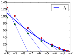
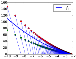
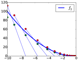
(a) $k=13,\ \alpha=1.3$	(b) $k=770,\ \alpha=1.99$	(c) $k=18,\ \alpha=1.3$
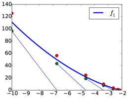
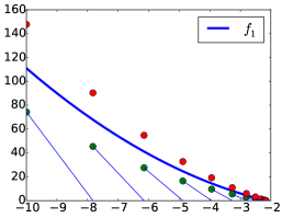
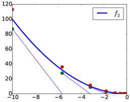
(d) $k=9,\ \alpha=1.3$	(e) $k=15,\ \alpha=1.99$	(f) $k=10,\ \alpha=1.3$

Figure 1: Inexact secant method (top row) and Newton method (bottom row) for root finding on the functions $f_{1}(\tau)=(\tau-1)^{2}-10$ (first two columns) and $f_{2}(\tau)=\tau^{2}$ (last column). Below each panel, $\alpha$ is the oracle accuracy, and $k$ is the number of iterations needed to converge, i.e., to reach $f_{i}(\tau_{k})\leq\epsilon$. For all problems, $\epsilon=10^{-2}$; the horizontal axis is $\tau$, and the vertical axis is $f_{i}(\tau)$.

2.2 Inexact Newton

The secant method can be improved by using approximate derivative information (when available) to design a Newton-type method. We design an inexact Newton method around an improved oracle that provides global linear under-estimators of $f$. This approach has two main advantages over the secant method. First, it is guaranteed to take longer steps than the inexact secant method. Second, it locally converges quadratically whenever $f$ is smooth, the values $f(\tau)$ are computed exactly, and the function has a nonzero (left) derivative at the minimal root. To formalize these ideas, we use the following strengthened version of an inexact evaluation oracle.

Definition 2.3 (Affine minorant oracle).

For a function $f:\mathbb{R}_{+}\to\mathbb{R}$, an affine minorant oracle is a mapping $\mathcal{O}_{f}$ that assigns to each pair $(t,\alpha)\in[f>0]\times[1,\infty)$ real numbers $(\ell,u,s)$ such that $0<\ell\leq f(\tau)\leq u$ and $u/\ell\leq\alpha$, and the affine function $\tau^{\prime}\mapsto\ell+s(\tau^{\prime}-\tau)$ globally minorizes $f$.

Algorithm 2 outlines a Newton method based on the affine minorant oracle. The inexact Newton method enjoys global convergence guarantees analogous to those of the inexact secant method, as described by Theorem 2.4; see Appendix A for the proof.

Data: Convex decreasing function $f\colon\mathbb{R}_{+}\to\mathbb{R}$ via an affine minorant oracle $\mathcal{O}_{f}$; target accuracy $\epsilon>0$; initial point $\tau_{0}$ with $f(\tau_{0})>0$; constant $\alpha\in(1,2)$.

$u_{-1}\leftarrow+\infty$

$k\leftarrow 0$

while $u_{k}>\epsilon$ do

       $(\ell_{k},u_{k},s_{k})\leftarrow\mathcal{O}_{f}(\tau_{k},\alpha)$

        [evaluate lower affine minorant oracle]

       $u_{k}\leftarrow\min\{u_{k},u_{k-1}\}$

        [ensure upper bound decreases]

       $\tau_{k+1}\leftarrow\tau_{k}-\ell_{k}/s_{k}$

        [Newton iteration]

       $k\leftarrow k+1$

return $\tau_{k}$

Algorithm 2 Inexact Newton method

Theorem 2.4 (Linear convergence of the inexact Newton method).

The inexact Newton method (Algorithm  2) terminates after at most

$$k\leq\max\left\{1+\log_{2/\alpha}\!\left(2C/\epsilon\right),\,2\right\}$$

iterations, where $C:=\max\{|s_{0}|(\tau_{*}-\tau_{0}),\,\ell_{0}\}$.

When we compare the two algorithms, it is easy to see that the Newton steps are never shorter than the secant steps. Indeed, let $(\ell_{k-1},u_{k-1},s_{k-1})=\mathcal{O}_{f}(\tau_{k-1},\alpha)$ and $(\ell_{k},u_{k},s_{k})=\mathcal{O}_{f}(\tau_{k},\alpha)$ be the triples returned by an affine minorant oracle at $\tau_{k-1}$ and $\tau_{k}$, respectively. Then

$$u_{k-1}\geq f(\tau_{k-1})\geq\ell_{k}+s_{k}(\tau_{k-1}-\tau_{k}),$$

which implies

$$s^{\hbox{\scriptsize secant}}_{k}:=(u_{k-1}-\ell_{k})/(\tau_{k-1}-\tau_{k})\leq s_{k}=:s^{\hbox{\scriptsize newton}}_{k}.$$

Therefore, the Newton step length $-\ell_{k}/s^{\hbox{\scriptsize newton}}_{k}$ is at least as large as the secant step length $-\ell_{k}/s^{\hbox{\scriptsize secant}}_{k}$.

As might be expected, the Newton method often outperforms the secant method in practice. The bottom row of panels in Figure 1 shows the progress of the Newton method on the same degenerate and nondegenerate test problems discussed earlier. Note in particular that the Newton method performs relatively well even when $\alpha$ is near its upper limit of 2; compare panels (b) and (e) in the figure. In this set of experiments, we chose an oracle with the same quality lower and upper bounds as the experiments with secant, but has the least favorable (i.e., steepest) slope that still results in a global minorant.

2.3 Lower minorants from duality

Under what circumstances are affine minorant oracles of the value function $v$ readily available? Not surprisingly, duality delivers an answer. Suppose we can express the value function in dual form

$$v(\tau)=\max_{y}\ \Phi(y,\tau),$$

where $\Phi$ is concave in $y$ and convex in $\tau$. For example, appealing to Fenchel duality, we may write

$$v(\tau) =\min_{x\in\mathcal{X}}\ \left\{\rho(Ax-b)\,\left|\ \varphi(x)\leq\tau\right.\right\}$$

$$=\min_{x\in\mathbb{R}^{n}}\ \rho(Ax-b)+\delta_{\mathcal{X}\cap\,[\varphi\leq\tau]}(x)$$

$$=\max_{y\in\mathbb{R}^{m}}\left\langle y,\,b\right\rangle-\rho^{\star}(-y)-\delta^{\star}_{\mathcal{X}\cap\,[\varphi\leq\tau]}(A^{T}\!y),$$

where the last equality holds provided that either the primal or the dual problem has a strictly feasible point [13, Theorem 3.3.5]. Hence, the Fenchel dual objective

$$\Phi(y,\tau):=\left\langle b,\,y\right\rangle-\rho^{\star}(-y)-\delta^{\star}_{\mathcal{X}\cap[\varphi\leq\tau]}(A^{T}\!y)$$ (2.1)

yields an explicit representation for $\Phi$. Note that convexity of $\Phi$ in $\tau$ is immediate; see Lemma A.2.

Many standard first-order methods that might be used as an oracle for evaluating $v(\bar{\tau})-\sigma$, generate both a lower bound $\bar{\ell}$ and a dual certificate $\bar{y}$ that satisfy the equation $\bar{\ell}=\Phi(\bar{y},\bar{\tau})-\sigma$. Examples include saddle-prox [54], Frank-Wolfe [35, 29], some projected (sub)gradient methods [4], and accelerated versions [64, 63, 56]. Whenever such a dual certificate $\bar{y}$ is available, we have

$$v(\tau)-\sigma\geq\Phi(\bar{y},\tau)-\sigma =\big{(}\Phi(\bar{y},\bar{\tau})-\sigma\big{)}+\big{(}\Phi(\bar{y},\tau)-\Phi(\bar{y},\bar{\tau})\big{)}$$ (2.2)

$$\geq\bar{\ell}+\bar{s}(\tau-\bar{\tau}),$$

where $\bar{s}$ is any subgradient of $\Phi$ at $(\bar{y},\bar{\tau})$ with respect to $\tau$. Hence, an inexact evaluation oracle that uses dual certificates can always be upgraded to an affine minorant oracle provided that an element of the subdifferential $\partial_{\tau}\Phi(y,\tau)$ can be evaluated. In the context of (2.1), this amounts to being able to compute an element of $\partial_{\tau}\delta^{\star}_{\mathcal{X}\cap\,[\varphi\leq\tau]}(A^{T}\!y)$. Reassuringly, such subdifferential formulas are readily available for a huge class of contemporary problems [3, Equations 4.1b, 6.5d, 6.20], and, in particular, for all the problems discussed in the rest of the paper.

In some instances, lower-bounds on the optimal value of $\mathcal{Q}_{\tau}$ provided by an algorithm are seemingly not related to a dual solution. A notable example of such a scheme is the Frank-Wolfe algorithm, which has recently received much attention. Supposing that the function $\rho$ is smooth, the Frank-Wolfe method applied to the problem $\mathcal{Q}_{\tau}$ iterates the following two steps:

$$\left\{\begin{aligned} z_{k}&\ =\ \mathop{\mathrm{argmin}}_{z\in\mathcal{X}\cap[\varphi\leq\tau]}~{}\langle A^{T}\nabla\rho(Ax_{k}-b),z\rangle\\ x_{k+1}&\ =\ x_{k}+t_{k}(z_{k}-x_{k})\end{aligned}\right.$$ (2.3)

for an appropriately chosen sequence of step-sizes $t_{k}$ (e.g., $t_{k}=\frac{2}{k+2}$). As the method progresses, it generates the upper bounds

$$u_{k}=\min_{i=1,\ldots,k}\rho(Ax_{i}-b)$$

on the optimal value of $\mathcal{Q}_{\tau}$. Moreover, it is easy to deduce from convexity that the following are valid lower bounds:

$$\ell_{k}=\max_{i=1,\ldots,k}\left\{\rho(Ax_{i}-b)+\langle A^{T}\nabla\rho(Ax_{i}-b),z_{i}-x_{i}\rangle\right\}.$$

Jaggi [35] provides an extensive discussion. If the step sizes $t_{k}$ are chosen appropriately, the gap satisfies $u_{k}-\ell_{k}\leq\mathcal{O}(D^{2}L/k)$, where the diameter $D$ of the feasible region and the Lipschitz constant $L$ of the gradient of the objective function of $\mathcal{Q}_{\tau}$ are measured in an arbitrary norm. Harchaoui, Juditsky, and Nemirovski [32] observe how to deduce from such lower bounds $\ell_{k}$ an affine minorant of the value function $v$, leading to a level-set scheme based on Newton’s method.

On the other hand, one can also show that the lower bounds $\ell_{k}$ are indeed generated by an explicit candidate dual solution, and hence the Frank-Wolfe algorithm (and its variants) fit perfectly in the above framework based on dual certificates. To see this, consider the Fenchel dual

$$\mathop{\hbox{maximize}}_{y\in\mathbb{R}^{m}}\quad\Phi(y,\tau)=\left\langle y,\,b\right\rangle-\rho^{\star}(-y)-\delta^{\star}_{\mathcal{X}\cap[\varphi\leq\tau]}(A^{T}\!y)$$

of $\mathcal{Q}_{\tau}$. Then for the candidate dual solutions $y_{i}:=-\nabla\rho(Ax_{i}-b)$, we successively deduce

$$\Phi(y_{i},\tau) =\langle y_{i},b\rangle-\rho^{\star}(-y_{i})-\langle A^{T}y_{i},z_{i}\rangle z_{i}$$ [definition of ]

$$=\langle y_{i},b\rangle+\Big{(}\rho(Ax_{i}-b)+\langle y_{i},Ax_{i}-b\rangle\Big{)}-\langle A^{T}y_{i},z_{i}\rangle$$ [Fenchel-Young inequality]

$$=\rho(Ax_{i}-b)+\langle A^{T}\nabla\rho(Ax_{i}-b),z_{i}-x_{i}\rangle.$$

Thus, the lower bounds $\ell_{k}$ are simply equal to $\ell_{k}=\max_{i=1,\ldots,k}\Phi(y_{i},\tau)$, and affine minorants on the value function $v$ are readily computed from the dual iterates $y_{k}$ and the derivatives $\partial_{\tau}\delta^{\star}_{\mathcal{X}\cap\,[\varphi\leq\tau]}(A^{T}\!y_{k})$.

3 Refinements

This section can be considered as an aside in our main exposition. Here, we address two questions that arise in the application of our root-finding approach: how best to apply the algorithm to problems with linear least-squares constraints, and how to recover a feasible point.

3.1 Least-squares misfit and degeneracy

Particularly important instances of problem $\mathcal{P}_{\sigma}$ arise when the misfit between $Ax$ and $b$ is measured by the 2-norm, i.e., $\rho=\|\cdot\|_{2}$. In this case, the objective of the level-set problem $\mathcal{Q}_{\tau}$ is $\|Ax-b\|_{2}$, which is not differentiable whenever $Ax=b$. Rather than applying a nonsmooth optimization scheme, an apparently easy fix is to replace the constraint in $\mathcal{P}_{\sigma}$ with its equivalent formulation $\tfrac{1}{2}\|Ax-b\|_{2}^{2}\leq\tfrac{1}{2}\sigma^{2}$, leading to the pair of problems

$$\displaystyle\mathop{\hbox{minimize}}_{x\in\mathcal{X}} \varphi(x) \mathop{\hbox{subject to}} \tfrac{1}{2}\|Ax-b\|_{2}^{2}\leq\tfrac{1}{2}\sigma^{2}, \mathcal{P}^{2}_{\sigma}$$ ()

$$\displaystyle\mathop{\hbox{minimize}}_{x\in\mathcal{X}} \tfrac{1}{2}\|Ax-b\|^{2} \mathop{\hbox{subject to}} \varphi(x)\leq\tau. \mathcal{Q}^{2}_{\tau}$$ ()

Throughout this section, the problems $\mathcal{P}_{\sigma}$ and $\mathcal{Q}_{\tau}$ continue to define the original formulations without the squares.

This straightforward adaptation, however, presents some numerical difficulties. Following the strategy outlined in the previous sections, the root finding procedure for $\mathcal{P}_{\sigma}^{2}$ would be automatically applied to the function

$$f_{2}(\tau):=\tfrac{1}{2}v^{2}(\tau)-\tfrac{1}{2}\sigma^{2},$$

where $v$ is the value function corresponding to the original (unsquared) level-set problem $\mathcal{Q}_{\tau}$. Clearly, the function $f_{2}$ is degenerate at each of its roots. As a result, the secant and Newton root-finding methods, respectively, would not converge locally superlinearly or quadratically—even if the values $v(\tau)$ are evaluated exactly. Moreover, we have observed empirically that this issue can in some cases cause numerical schemes to stagnate.

A simple alternative avoids this pitfall: apply the root-finding procedure to the function

$$f_{1}(\tau):=v(\tau)-\sigma$$

corresponding to the value function of $\mathcal{Q}_{\tau}$, but solve $\mathcal{Q}_{\tau}^{2}$ to approximately evaluate $f_{2}$ and consequently to approximately evaluate $f_{1}$. The oracle definitions required for the secant (Algorithm 1) and Newton (Algorithm 2) methods require suitable modification. For secant, the modifications are straightforward, but for Newton, care is needed in order to obtain the correct affine minorants of $f_{1}$ from those of $f_{2}$. The required modifications are described in turn below.

Secant

For the secant method applied to the function $f_{1}$, we derive an inexact evaluation oracle from an inexact evaluation oracle for $f_{2}$ as follows. Suppose that we have approximately solved $\mathcal{Q}_{\tau}^{2}$ by an inexact-evaluation oracle

$$\mathcal{O}_{f_{2}}\big{(}\tau,\alpha^{2}\big{)}=\left(\tfrac{1}{2}\ell^{2}-\tfrac{1}{2}\sigma^{2},\ \tfrac{1}{2}u^{2}-\tfrac{1}{2}\sigma^{2}\right),$$ (3.1)

where we have specified the relative accuracy between the lower and upper bounds to be $\alpha^{2}$. Assume, without loss of generality, that $u,\ell\geq 0$. Then clearly $u$ and $\ell$ are upper and lower bounds on $v(\tau)$, respectively. It is now straightforward to deduce

$$0\leq\ell-\sigma\leq f_{1}(\tau)\leq u-\sigma\qquad\hbox{and}\qquad\frac{u-\sigma}{\ell-\sigma}\leq\sqrt{\frac{u^{2}-\sigma^{2}}{\ell^{2}-\sigma^{2}}}\leq\alpha.$$ (3.2)

Hence an inexact function evaluation oracle for $f_{2}$ yields an inexact evaluation oracle for $f_{1}$.

Newton

Newton’s method in this setting is slightly more intricate: the nuance is in obtaining a valid affine minorant of $f_{1}$. We use the respective objectives of the dual problems corresponding to $\mathcal{Q}_{\tau}$ and $\mathcal{Q}_{\tau}^{2}$, given by

$$\Phi_{1}(y,\tau) :=\left\langle b,\,y\right\rangle-\delta^{\star}_{\mathcal{X}\cap[\varphi\leq\tau]}(A^{T}y)-\delta_{\mathbb{B}_{2}}(y),$$

$$\Phi_{2}(y,\tau) :=\left\langle b,\,y\right\rangle-\delta^{\star}_{\mathcal{X}\cap[\varphi\leq\tau]}(A^{T}y)-\tfrac{1}{2}\|y\|^{2}_{2}.$$

As described by (3.1), an inexact solution of $\mathcal{Q}_{\tau}^{2}$ delivers values $\ell$ and $u$ that satisfy (3.2). Suppose that the oracle additionally delivers a dual certificate $y$ that satisfies $\Phi_{2}(y,\tau)=\tfrac{1}{2}\ell^{2}$. Let $s\in\partial_{\tau}\Phi_{2}(y,\tau)$ be any subgradient. The following result establishes that

$$(\hat{\ell},\,u,\,s/\|y\|_{2})\hbox{\qquad with\qquad}\hat{\ell}:=\Phi_{1}\left(y/\|y\|_{2},\,\tau\right),$$

defines a valid affine minorant for $f_{1}$.

Proposition 3.1.

The inequalities

$$0\leq\hat{\ell}-\sigma\leq f_{1}(\tau)\leq u-\sigma\qquad\hbox{and}\qquad(u-\sigma)/(\hat{\ell}-\sigma)\leq\alpha$$

hold, and the linear functional $\tau^{\prime}\mapsto(\hat{\ell}-\sigma)-(s/\|y\|_{2})(\tau^{\prime}-\tau)$ minorizes $f_{1}$.

The proof is given in Appendix A. In summary, if we wish to obtain a super-optimal and $\epsilon$-feasible solution to $\mathcal{P}_{\sigma}$, in each iteration of the Newton method we must evaluate $f_{2}(\tau)$ up to an absolute error of at most $\frac{1}{2}(1-1/\alpha)^{2}\epsilon^{2}$. Indeed, suppose that in the process of evaluation, the oracle $\mathcal{O}_{f_{2}}\big{(}\tau,\alpha^{2}\big{)}$ achieves $u$ and $l$ satisfying

$$\tfrac{1}{2}u^{2}-\tfrac{1}{2}\ell^{2}\leq\tfrac{1}{2}(1-1/\alpha)^{2}\epsilon^{2}.$$

Then we obtain the inequality

$$u-\ell=\sqrt{(u-\ell)^{2}}\leq\sqrt{u^{2}-\ell^{2}}\leq(1-1/\alpha)\epsilon,$$

Thus, by the discussion following Definition 2.1, either the whole Newton scheme can now terminate with $f_{1}(\tau)\leq\epsilon$ or we have achieved the relative accuracy $(u-\sigma)/(\ell-\sigma)\leq\alpha$ for the oracle.

3.2 Recovering feasibility

A potential shortcoming of the level-set approach is that the computed solutions are only $\epsilon$-feasible. Some applications may demand feasible solutions. A straightforward remedy is to project the computed $\epsilon$-feasible point onto the original constraint set $\left\{x\in\mathcal{X}\,\left|\ \rho(Ax-b)\leq\sigma\right.\right\}.$ However, this operation can be computationally impractical; for example, access to the matrix $A$ is often only available through matrix vector products. An alternative is provided by Renegar [60], who suggests an inexpensive radial-projection scheme for conic optimization that generates a feasible point while still preserving some notion of optimality. The approach requires knowledge of a point $e$ strictly feasible for the original problem, and obtains a feasible point $x$ whose optimality is measured with respect to $e$, i.e.,

$$\frac{\varphi(x)-\hbox{OPT}}{\varphi(e)-\hbox{OPT}}\leq\delta$$

for some small positive parameter $\delta$.

To explain the approach, fix some target $\delta<1$ and suppose that $e\in\mathcal{X}$ is strictly feasible for $\mathcal{P}_{\sigma}$, i.e.,

$$\rho(Ae-b)<\sigma.$$

Suppose also that a point $z\in\mathcal{X}$ is super-optimal and $\epsilon$-feasible for $\mathcal{P}_{\sigma}$:

$$\varphi(z)\leq\textrm{OPT}\quad\textrm{ and }\quad\sigma<\rho(Az-b)\leq\sigma+\epsilon,\hbox{\qquad with\qquad}\epsilon:=\delta\big{[}\sigma-\rho(Ae-b)\big{]}.$$

These relationships imply the inequality

$$\alpha:=\frac{\rho(Az-b)-\sigma}{\rho(Az-b)-\rho(Ae-b)}\leq\delta.$$

Set $x:=z+\alpha(e-z)$, which is the radial projection of $z$ towards the feasible point $e$. It follows from convexity that $\varphi(x)\leq(1-\alpha)\varphi(z)+\alpha\varphi(e)$. Subtract OPT from both sides and rearrange terms to obtain

$$\frac{\varphi(x)-\hbox{OPT}}{\varphi(e)-\hbox{OPT}}\leq(1-\alpha)\frac{\varphi(z)-\hbox{OPT}}{\varphi(e)-\hbox{OPT}}+\alpha\leq\alpha\leq\delta.$$

It only remains to show that the radial projection $x$ is feasible. The inclusion $x\in\mathcal{X}$ follows from convexity of $\mathcal{X}$. Use the definition of $\alpha$, together with the convexity of $\rho$, to obtain

$$\rho(Ax-b)\leq\rho(Az-b)-\alpha[\rho(Az-b)-\rho(Ae-b)]=\sigma,$$

which establishes feasibility of $x$.

4 Some problem classes

There is a surprising variety of useful problems that can be treated by the root-finding approach. These include problems from sparse optimization, with applications in compressed sensing and sparse recovery, generalized linear models, which feature prominently in statistical applications, and conic optimization, which includes semidefinite programming. The following sections are in some sense a “cookbook” that describes how features of particular problems can be combined to apply the root-finding approach. In some cases, such as with conic optimization, we have the opportunity to derive unexpected algorithms.

4.1 Conic optimization

The general conic problem (CP) has the form

$$\mathop{\hbox{minimize}}_{x}\quad\left\langle c,\,x\right\rangle\quad\mathop{\hbox{subject to}}\quad{\mathcal{A}}x=b,\ x\in{\mathcal{K}},$$ (CP)

where ${\mathcal{A}}:E_{1}\to E_{2}$ is a linear map between Euclidean spaces, and ${\mathcal{K}}\subset E_{1}$ is a proper, closed, convex cone. The familiar forms of this problem include linear programming (LP), second-order cone programming (SOCP), and semidefinite programming (SDP). Ben-Tal and Nemirovski [6] survey an enormous number of applications and formulations captured by conic programming.

There are at least two possible approaches for applying the level-set framework. The first exchanges the roles of the original objective $\left\langle c,\,x\right\rangle$ with the linear constraint $Ax=b$, and brings a least-squares term into the objective; the second approach moves the cone constraint $x\in{\mathcal{K}}$ into the objective via a kind of distance function. This yields two distinct algorithms for the conic problem. The two approaches are summarized in Table 1. Note that it is possible to consider conic problems with the more general constraint $\rho(Ax-b)\leq\sigma$, but here we restrict our attention to the simpler affine constraint, which conforms to the standard form of conic optimization.

Problem	$\mathcal{P}_{\sigma}$	$\mathcal{Q}_{\tau}$	Dual of $\mathcal{Q}_{\tau}$
CP least-squares level	$\begin{array}[t]{cl}\displaystyle\min_{x}&\left\langle c,\,x\right\rangle\\ \hbox{s.t.}&\begin{aligned} {\mathcal{A}}x&=b\\ x&\in{\mathcal{K}}\end{aligned}\end{array}$	$\begin{array}[t]{cl}\displaystyle\min_{x}&\|{\mathcal{A}}x-b\|_{2}\\ \hbox{s.t.}&\begin{aligned} \left\langle c,\,x\right\rangle&\leq\tau\\ x&\in{\mathcal{K}}\end{aligned}\end{array}$	$\begin{array}[t]{cl}\displaystyle\max_{y,\ \mu\geq 0}&\left\langle b,\,y\right\rangle-\mu\tau\\ \hbox{s.t.}&\begin{aligned} \|y\|_{2}&\leq 1\\ \mu c-{\mathcal{A}}^{*}y&\in\mathcal{K}^{*}\end{aligned}\end{array}$
CP cone level	$\begin{array}[t]{cl}\displaystyle\min_{x}&\left\langle c,\,x\right\rangle\\ \textrm{s.t.}&\begin{aligned} {\mathcal{A}}x&=b\\ x&\in\mathcal{K}\end{aligned}\end{array}$	$\begin{array}[t]{cl}\displaystyle\min_{x}&-\lambda_{\min}(x)\\ \textrm{s.t.}&\begin{aligned} {\mathcal{A}}x&=b\\ \left\langle c,\,x\right\rangle&\leq\tau\end{aligned}\end{array}$	$\begin{array}[t]{cl}\displaystyle\max_{y,\ \mu\geq 0}&\left\langle b,\,y\right\rangle-\mu\tau\\ \textrm{s.t.}&\begin{aligned} \left\langle\mu c-\mathcal{A}^{*}y,\,e\right\rangle&=1\\ \mu c-{\mathcal{A}}^{*}y&\in\mathcal{K}^{*}\end{aligned}\end{array}$

Table 1: Least-squares and conic level-set problems for conic optimization. In these examples, we require ${\mathcal{A}}x=b$.

4.1.1 First approach: least-squares level set

To get started with this approach, we make the blanket assumption that we know a strictly feasible vector ${\widehat{y\mkern 2.0mu}\mkern-2.0mu}{}$ for the dual of (CP):

$$\mathop{\hbox{maximize}}_{y}\quad\left\langle b,\,y\right\rangle\quad\mathop{\hbox{subject to}}\quad c-\mathcal{A}^{*}y\in{\mathcal{K}}^{*}.$$

Thus ${\widehat{y\mkern 2.0mu}\mkern-2.0mu}{}$ satisfies ${\widehat{c\mkern 3.0mu}\mkern-3.0mu}{}:=c-{\mathcal{A}}^{*}{\widehat{y\mkern 2.0mu}\mkern-2.0mu}{}\in\operatorname{int}\mathcal{K}^{*}$. A simple calculation shows that minimizing the new objective $\left\langle{\widehat{c\mkern 3.0mu}\mkern-3.0mu}{},\,x\right\rangle$ only changes the objective of CP by a constant: for all $x$ feasible for CP, we now have

$$\left\langle{\widehat{c\mkern 3.0mu}\mkern-3.0mu}{},\,x\right\rangle=\left\langle c,\,x\right\rangle-\left\langle{\mathcal{A}}x,\,{\widehat{y\mkern 2.0mu}\mkern-2.0mu}{}\right\rangle=\left\langle c,\,x\right\rangle-\left\langle b,\,{\widehat{y\mkern 2.0mu}\mkern-2.0mu}{}\right\rangle.$$

In particular, we may assume $b\neq 0$, since otherwise, the origin is the trivial solution for the shifted problem. Note that in the important case $c\in\operatorname{int}\mathcal{K}$, we can simply set ${\widehat{y\mkern 2.0mu}\mkern-2.0mu}{}=0$, which yields the equality $c={\widehat{c\mkern 3.0mu}\mkern-3.0mu}{}$.

We now illustrate the computational complexity of applying the root-finding approach to solve (CP) using the level-set problem

$$\mathop{\hbox{minimize}}_{x}\quad\|{\mathcal{A}}x-b\|_{2}\quad\mathop{\hbox{subject to}}\quad\left\langle{\widehat{c\mkern 3.0mu}\mkern-3.0mu}{},\,x\right\rangle\leq\tau,\ x\in{\mathcal{K}}.$$ (4.1)

Our aim is then to find a root of (1.2), where $v$ is the value function of (4.1). The top row of Table 1, gives the corresponding dual

$$\mathop{\hbox{maximize}}_{y,~{}\,\mu\geq 0}\quad\left\langle b,\,y\right\rangle-\mu\tau\quad\mathop{\hbox{subject to}}\quad\|y\|_{2}\leq 1,\ \mu c-{\mathcal{A}}^{*}y\in\mathcal{K}^{*}$$

of the level-set problem. We use $\tau_{0}=0$ as the initial root-finding iterate. Because of the inclusion ${\widehat{c\mkern 3.0mu}\mkern-3.0mu}{}\,\in\operatorname{int}\mathcal{K}^{*}$, we deduce that $x=0$ is the only feasible solution to (4.1), which yields $v(0)=\|b\|_{2}$ and the exact lower bound $\ell_{0}=\|b\|_{2}$. The corresponding dual certificate is $(\bar{y},\bar{\mu})=(b/\|b\|_{2},\bar{\mu})$, where

$$\bar{\mu}:=\min_{\mu}\left\{\mu{\widehat{c\mkern 3.0mu}\mkern-3.0mu}{}-\frac{\mathcal{A}^{*}b}{\|b\|_{2}}\in{\mathcal{K}}^{*}\right\}.$$ (4.2)

Note the inequality $\bar{\mu}>0$, because otherwise we would deduce $\mathcal{A}^{*}b\in-\mathcal{K}^{*}$, implying the inequality $\|b\|^{2}_{2}=\langle b,\mathcal{A}x\rangle=\langle\mathcal{A}^{*}b,x\rangle\leq 0$ for any feasible $x$. This contradicts our assumption that $b$ is nonzero. In the case where ${\mathcal{K}}$ is the nonnegative orthant and ${\widehat{c\mkern 3.0mu}\mkern-3.0mu}{}=e$, the number $\bar{\mu}$ is simply the maximal coordinate of $\mathcal{A}^{*}b/\|b\|_{2}$; if ${\mathcal{K}}$ is the semidefinite cone and ${\widehat{c\mkern 3.0mu}\mkern-3.0mu}{}=I$, the number $\bar{\mu}$ is the right-most eigenvalue of $\mathcal{A}^{*}b/\|b\|_{2}$. With these values, Theorem 2.4 asserts that within $\mathcal{O}\big{(}\log_{2/\alpha}2C/\epsilon\big{)}$ inexact Newton iterations, where $\alpha$ is the accuracy of each subproblem solve and

$$C=\max\left\{\bar{\mu}\cdot\left(\text{OPT}-\langle b,{\widehat{y\mkern 2.0mu}\mkern-2.0mu}{}\rangle\right),\|b\|_{2}\right\},$$

the point $x\in\mathcal{K}$ that yields the final upper bound in (4.1) is a super-optimal and $\epsilon$-feasible solution of the shifted CP, i.e.,

$$\langle{\widehat{c\mkern 3.0mu}\mkern-3.0mu}{},x\rangle\leq\hbox{OPT}-\langle{\widehat{y\mkern 2.0mu}\mkern-2.0mu}{},b\rangle\qquad\textrm{ and }\qquad\|\mathcal{A}x-b\|_{2}\leq\epsilon.$$

To see how good the obtained point $x$ is for the original CP (without the shift), note that

$$\langle{\widehat{c\mkern 3.0mu}\mkern-3.0mu}{},x\rangle=\langle c,x\rangle-\langle\mathcal{A}^{*}{\widehat{y\mkern 2.0mu}\mkern-2.0mu}{},x\rangle=\langle c,x\rangle-\langle{\widehat{y\mkern 2.0mu}\mkern-2.0mu}{},\mathcal{A}x-b\rangle-\langle{\widehat{y\mkern 2.0mu}\mkern-2.0mu}{},b\rangle\geq\langle c,x\rangle-\langle{\widehat{y\mkern 2.0mu}\mkern-2.0mu}{},b\rangle-\epsilon\|{\widehat{y\mkern 2.0mu}\mkern-2.0mu}{}\|_{2},$$

and hence $\langle c,x\rangle\leq\hbox{OPT}+\epsilon\|{\widehat{y\mkern 2.0mu}\mkern-2.0mu}{}\|_{2}$. In particular, in the important case where $c\in\operatorname{int}{\mathcal{K}}^{*}$, we deduce super-optimality $\langle c,x\rangle\leq\hbox{OPT}$ for the target problem CP.

Each Newton root-finding iteration requires an approximate solution of (4.1). As described in §3.1, we obtain this approximation by instead solving its smooth formulation with the squared objective $\tfrac{1}{2}\|{\mathcal{A}}x-b\|_{2}^{2}$. Let $L:=\|{\mathcal{A}}\|_{2}^{2}$ be the Lipschitz constant for the gradient ${\mathcal{A}}^{T}({\mathcal{A}}x-b)$, and let $D$ be the diameter of the region $\{x\mid\left\langle{\widehat{c\mkern 3.0mu}\mkern-3.0mu}{},\,x\right\rangle=1,\ x\in{\mathcal{K}}\}$, which is finite by the inclusion ${\widehat{c\mkern 3.0mu}\mkern-3.0mu}{}\in\operatorname{int}{\mathcal{K}}^{*}$. Thus, in order to evaluate $v$ to an accuracy $\epsilon$, we may apply an accelerated projected-gradient method on the squared version of the problem to an additive error of $\frac{1}{2}(1-1/\alpha)^{2}\epsilon^{2}$ (see end of §3.1), which terminates in at most

$$\mathcal{O}\left(\frac{\sqrt{L}\cdot\tau D}{\epsilon(1-1/\alpha)}\right)=\mathcal{O}\left(\frac{\|A\|_{2}\cdot D\cdot\left(\hbox{OPT}-\langle b,{\widehat{y\mkern 2.0mu}\mkern-2.0mu}{}\rangle\right)}{\epsilon(1-1/\alpha)}\right)$$

iterations [7, §6.2]. Here, we have used the monotonicity of the root finding scheme to conclude $\tau\leq\hbox{OPT}-\langle b,{\widehat{y\mkern 2.0mu}\mkern-2.0mu}{}\rangle$. When $\mathcal{K}$ is the non-negative orthant, each projection can be accomplished with $\mathcal{O}(n)$ floating point operations [15], while for the semidefinite cone each projection requires an eigenvalue decomposition. More generally, such projections can be quickly found as long as projections onto the cone $\mathcal{K}$ are available; see Remark A.5. We note that an improved complexity bound can be obtained for the oracles in the LP and SDP cases by replacing the Euclidean projection step with a Bregman projection derived from the entropy function; see e.g., Beck and Teboulle [5] or Tseng [64, §3.1]. We leave the details to the reader.

Figure 2: Progress of the root-finding method for a linear program. The panels on the left depict the graph of $v(\tau)$ (solid line), and the squares and circles, respectively, show the upper and lower bounds computed using an optimal projected-gradient method. The horizontal log scale results in a value function that appears nonconvex. The panels on the right show the number of projected-gradient iterations for each Newton step. Top panels: $\alpha=1.8$. Bottom panels: $\alpha=1.01$.

In summary, we can obtain a point $x\in\mathcal{K}$ that satisfies

$$\langle c,x\rangle\leq\hbox{OPT}+\epsilon\|{\widehat{y\mkern 2.0mu}\mkern-2.0mu}{}\|_{2}\qquad\textrm{ and }\qquad\|{\mathcal{A}}x-b\|_{2}\leq\epsilon$$

in at most

$$\mathcal{O}\left(\frac{\|A\|_{2}\cdot D\cdot\left(\hbox{OPT}-\langle b,{\widehat{y\mkern 2.0mu}\mkern-2.0mu}{}\rangle\right)}{\epsilon(1-1/\alpha)}\right)\cdot\mathcal{O}\left(\log_{2/\alpha}\frac{\max\left\{\bar{\mu}\cdot\left(\text{OPT}-\langle b,{\widehat{y\mkern 2.0mu}\mkern-2.0mu}{}\rangle\right),\|b\|_{2}\right\}}{\epsilon}\right)$$

iterations of an accelerated projected-gradient method, where $\bar{\mu}$ is defined in (4.2). Reassuringly, the complexity bound depends on all the expected quantities.

4.1.2 Second approach: conic level set

Renegar’s recent work [60] on conic optimization inspires a possible second level-set approach based on interchanging the roles of the affine objective and the conic constraint in (CP). A key step is to define a convex function $\kappa$ that is nonnegative on the cone ${\mathcal{K}}$, and positive elsewhere, so that it acts as a surrogate for the conic constraint, i.e.,

$$\kappa(x)\leq 0\hbox{\qquad if and only if\qquad}x\in{\mathcal{K}}.$$ (4.3)

The conic optimization problem then can be expressed equivalently in entirely functional form as

$$\mathop{\hbox{minimize}}_{x}\quad\left\langle c,\,x\right\rangle\quad\mathop{\hbox{subject to}}\quad{\mathcal{A}}x=b,\ \kappa(x)\leq 0,$$ (4.4)

which allows us to define the level-set problem

$$\mathop{\hbox{minimize}}_{x}\quad\kappa(x)\quad\mathop{\hbox{subject to}}\quad{\mathcal{A}}x=b,\ \left\langle c,\,x\right\rangle\leq\tau.$$ (4.5)

Renegar gives a procedure for constructing a suitable surrogate function $\kappa$ under the assumption that ${\mathcal{K}}$ has a nonempty interior: choose a point $e\in\operatorname{int}{\mathcal{K}}$ and define $\kappa(x)=-\lambda_{\min}(x)$, where

$$\lambda_{\min}(x):=\inf\,\{\lambda\mid x-\lambda e\not\in{\mathcal{K}}\}.$$

In the case of the PSD cone, we may take $e=I$, and then $\lambda_{\min}$ yields the minimum eigenvalue function, which explains the notation. As is shown in [60, Prop. 2.1], the function $\lambda_{\min}$ is Lipschitz continuous (with modulus one) and concave, as would be necessary to apply a subgradient method for minimizing $\kappa$. Renegar derives a novel algorithm along with complexity bounds for CP using the $\lambda_{\min}$ function. A rigorous methodology for applying the level-set scheme, as described in the current paper, requires further research. It is an intriguing research agenda to unify Renegar’s explicit complexity bounds with the proposed level-set approach. We note in passing that the dual of the resulting level-set problem, needed to apply the lower affine-minorant root-finding method, is shown in the second row of Table 1, and can be derived using the conjugate of $\lambda_{\min}$; see Lemma A.3.

In principle, the main requirement of our level-set approach is that the surrogate function that satisfies (4.3) yields the equivalent formulation (4.4). Depending on the algorithms available for solving the level-set problem (4.5), it may be convenient to define a function $\kappa$ with certain useful properties. For example, we might choose to define the differentiable surrogate function

$$\kappa=\tfrac{1}{2}\hbox{dist}_{\mathcal{K}}^{2},\hbox{\qquad where\qquad}\hbox{dist}_{\mathcal{K}}(x):=\inf_{z\in{\mathcal{K}}}\ \|x-z\|$$

measures the distance to the cone ${\mathcal{K}}$.

Note the significant differences between the least-squares and conic level-set problems (4.1) and (4.5). For the sake of discussion, suppose that ${\mathcal{K}}$ is the positive semidefinite cone. The least-squares level-set problem has a smooth objective whose gradient can be easily computed by applying the operator ${\mathcal{A}}$ and its adjoint, but the constraint set still contains the explicit cone. Projected-gradient methods, for example, require a full eigenvalue decomposition of the steepest-descent step, while the Frank-Wolfe method requires only a single rightmost eigenpair computation. The latter level-set problem, however, can require a potentially more complex procedure to compute a gradient or subgradient, but has an entirely linear constraint set. In this case, projected (sub)gradient methods require a least-squares solve for the projection step.

4.2 Gauge optimization

In this section, we illustrate the general applicability of the level-set approach to regularized data-fitting problems by restricting the convex functions $\varphi$ and $\rho$ to be gauges—i.e., functions that are additionally nonnegative, positively homogeneous, and vanish at the origin. Throughout, we assume that the side constraint $x\in\mathcal{X}$ is absent from the formulation $\mathcal{P}_{\sigma}$. A large class of problems of this type occurs in sparsity optimization. Basis pursuit (and its “denoising” variant BP_σ) [22] was our very first example in §1, and many related problems can be similarly expressed. The first two columns of Table 2 describe various formulations of current interest, including basis pursuit denoising (BPDN), low-rank matrix recovery [28, 18], a sharp version of the elastic-net problem [73], and gauge optimization [30] in its standard form. The third column shows the level-set problem $\mathcal{Q}_{\tau}$ needed to evaluate the value function $v(\tau)$, while the fourth column shows the slopes needed to implement the Newton scheme.

The dual representation (2.1) can be specialized for this family, and requires some basic facts regarding a gauge function $f$ and its polar

$$f^{\circ}(y):=\inf\left\{\mu>0\,\left|\ \left\langle x,\,y\right\rangle\leq\mu f(x)\mbox{ for all }x\right.\right\}.$$

When $f$ is a norm, the polar $f^{\circ}$ is simply the familiar dual norm. There is a close relationship between gauges, their polars, and the support functions of their sublevel sets, as described by the identities [30, Prop. 2.1(iv)]

$$f^{\circ}=\delta^{\star}_{[f\leq 1]}\quad\hbox{and}\quad f^{\star}=\delta_{[f^{\circ}\leq 1]}.$$

We apply these identities to the quantities involving $\rho$ and $\varphi$ in the expression for the dual representation $\Phi$ in (2.1), and deduce

$$\delta^{\star}_{[\varphi\leq\tau]}=\tau\delta^{\star}_{[\varphi\leq 1]}=\tau\varphi^{\circ}\quad\hbox{and}\quad\rho^{\star}=\delta_{[\rho^{\circ}\leq 1]}.$$

Substitute these into $\Phi$ to obtain the equivalent expression

$$\Phi(y,\tau)=\left\langle b,\,y\right\rangle-\delta_{[\rho^{\circ}\leq 1]}(-y)-\tau\varphi^{\circ}(A^{T}y).$$

We can now write an explicit dual for the level-set problem $\mathcal{Q}_{\tau}$:

$$\mathop{\hbox{maximize}}_{y}\quad\left\langle b,\,y\right\rangle-\tau\varphi^{\circ}(A^{T}y)\quad\mathop{\hbox{subject to}}\quad\rho^{\circ}(-y)\leq 1.$$ (4.6)

In the last three rows of the table, we set $\rho=\|\cdot\|_{2}$, which is self polar. For BPDN, we use the vector 1-norm $\varphi=\|\cdot\|_{1}$, whose polar is the dual norm $\varphi^{\circ}=\|\cdot\|_{\infty}$. For matrix completion, the function $\varphi=\|\cdot\|_{*}:=\sum_{i=1}^{\min\{m,n\}}\sigma_{i}(\cdot)$ is the nuclear norm of a $n$-by-$m$ matrix, which is polar to the spectral norm $\varphi^{\circ}=\sigma_{{}_{\max}}(\cdot)$. For the sharp elastic net, we use Lemma A.4 to deduce

$$(\alpha\|\cdot\|_{1}+\beta\|\cdot\|_{2})^{\circ}=(\gamma_{\frac{1}{\alpha}\mathbb{B}_{1}}+\gamma_{\frac{1}{\beta}\mathbb{B}_{2}})^{\circ}=\gamma_{\left(\frac{1}{\alpha}\mathbb{B}_{1}\right)^{\circ}+\left(\frac{1}{\beta}\mathbb{B}_{2}\right)^{\circ}}=\gamma_{\alpha\mathbb{B}_{\infty}+\beta\mathbb{B}_{2}}.$$

A distinctive feature of all of the problems stated in Table 2 is the nondifferentiability of the objective of $\mathcal{Q}_{\tau}$. The choice seems especially peculiar when $\rho$ is the 2-norm, since in that case, it is obvious that an equivalent smooth problem can be obtained by simply squaring the objective $\mathcal{Q}_{\tau}$ and the corresponding constraint in the original problem $\mathcal{P}_{\sigma}$. Of course, we do not prescribe the method for solving the level-set problem, and depending on the application and solvers available, it may be more convenient or efficient to solve a smooth variant of $\mathcal{Q}_{\tau}$ in order to obtain a solution of the nonsmooth version; cf. §3.1.

Problem	$\mathcal{P}_{\sigma}$	$\mathcal{Q}_{\tau}$	$\partial_{\tau}\Phi(y,\tau)$
$\begin{array}[t]{@{}ll@{}}\rm gauge\\ \rm optimization\end{array}$	$\begin{array}[t]{cl@{}}\displaystyle\min_{x}&\varphi(x)\\ \textrm{s.t.}&\rho(Ax-b)\leq\sigma\end{array}$	$\begin{array}[t]{cl@{}}\displaystyle\min_{x}&\rho(Ax-b)\\ \textrm{s.t.}&\varphi(x)\leq\tau\end{array}$	$-{\varphi^{\circ}(A^{T}y)}$
BPDN	$\begin{array}[t]{cl@{}}\displaystyle\min_{x}&\|x\|_{1}\\ \textrm{s.t.}&\|Ax-b\|_{2}\leq\sigma\end{array}$	$\begin{array}[t]{cl@{}}\displaystyle\min_{x}&\|Ax-b\|_{2}\\ \textrm{s.t.}&\|x\|_{1}\leq\tau\end{array}$	${-\|{A^{T}y\|_{\infty}}}$
$\begin{array}[t]{@{}ll@{}}\hbox{sharp}\\ \hbox{elast-net}\end{array}$	$\begin{array}[t]{cl@{}}\displaystyle\min_{x}&\alpha\|x\|_{1}+\beta\|x\|_{2}\\ \textrm{s.t.}&\|Ax-b\|_{2}\leq\sigma\end{array}$	$\begin{array}[t]{cl@{}}\displaystyle\min_{x}&\|Ax-b\|_{2}\\ \textrm{s.t.}&\alpha\|x\|_{1}+\beta\|x\|_{2}\leq\tau\end{array}$	$-{\gamma_{\alpha\mathbb{B}_{\infty}+\beta\mathbb{B}_{2}}(A^{T}\!y)}$
$\begin{array}[t]{@{}ll@{}}\rm matrix\\ \rm completion\end{array}$	$\begin{array}[t]{cl@{}}\displaystyle\min_{X}&\|X\|_{*}\\ \textrm{s.t.}&\|{\mathcal{A}}X-b\|_{2}\leq\sigma\end{array}$	$\begin{array}[t]{cl@{}}\displaystyle\min_{x}&\|{\mathcal{A}}X-b\|_{2}\\ \textrm{s.t.}&\|X\|_{*}\leq\tau\end{array}$	$-{\sigma_{1}({\mathcal{A}}^{*}y)}$

Table 2: Nonsmooth regularized data-fitting.

4.3 Generalized linear models

In all the examples we have seen so far, we have encountered only two types of misfit functions $\rho$, namely the squared 2-norm and the various gauges listed in Table 2. In this section, we broaden the scope by exploring several examples arising from statistical modeling. In particular, we consider the broad class of generalized linear models (GLMs) [52], which capture non-Gaussian data—including non-negative, count, boolean and multinomial variables—and robust log-concave densities.

GLMs assume that the observed data is distributed according to a member of the exponential family, and postulate a linear predictive model for key parameters. Suppose we are given data pairs $\{(b_{i},a_{i})\}^{n}_{i=1}\subset\mathbb{R}\times\mathbb{R}^{m}$, where $b_{i}$ is an observation associated with the covariate vector $a_{i}$ for individual $i=1,\ldots,n$. GLMs assume that the postulated density for each response $b_{i}$ is the function

$$p(b_{i};\,\theta_{i})=C(b_{i},\phi)\exp\left(\frac{b_{i}\theta_{i}-c(\theta_{i})}{\phi}\right),$$ (4.7)

where $\phi$ is the dispersion parameter, $\theta_{i}$ is the mean parameter, $c(\cdot)$ is a function that specifies the distribution, and $C(b_{i},\phi)$ is a normalization constant that can depend on the data and $\phi$. To simplify the exposition, we focus only on the canonical parameter $\theta_{i}$, and assume that the dispersion parameter $\phi$ is known and present in its simplest form; see McCullah and Nelder [52] for more general cases. Whenever the function $c$ is convex, it is clear that the resulting density is log-concave. To complete the GLM specification, one now assumes that $b_{i}$ is distributed according to the GLM in (4.7) with

$$\theta_{i}=a_{i}^{T}x,$$

where $x$ is an unknown vector that is uniform across the population from which the data is selected. The task is to infer the vector $x$ from the given data.

A technical concept in GLM modeling is the link function—an invertible function that maps likelihood parameters to the canonical parameter $\theta_{i}$. For example, when working with count data, one encounters the Poisson distribution, which is proportional to $\exp(b_{i}\log\lambda_{i}-\lambda_{i})$. We identify (4.7) with this distribution using the log link function, and set $\theta_{i}=\log\lambda_{i}$. It necessarily follows that $c(\theta_{i})=\exp(\theta_{i})$.

Assuming that the data is chosen independently from the population, the negative log-likelihood function for this model is given by

$$L(b;Ax)=\sum^{n}_{i=1}-{\ln p(b_{i};a_{i}^{T}x)},$$

where $a_{i}$ the $i$th row of the matrix $A$. The likelihood-constrained formulation $\mathcal{P}_{\sigma}$ for the regularized GLM is thus given by the problem

$$\mathop{\hbox{minimize}}_{x}\quad\varphi(x)\quad\text{subject to}\quad L(b;Ax)\leq\sigma,$$ (4.8)

where $\varphi$ is a given regularizer. For example, the 1-norm regularizer may be used to induce sparsity in the parameter $x$. A reasonable choice for $\sigma$ is a proportion of the expectation:

$$\sigma\propto\mathbb{E}\,L(b;\,Ax).$$ (4.9)

When an estimate of the expectation is not available, $\sigma$ can be selected by using an expected variance-reduction scheme, so that $\sigma\propto L(b;0)$, where the proportionality constant is chosen based on practitioner-prior experience.

Applying the level-set approach.

We now describe the various ingredients needed to apply the level-set approach to the GLM family. For simplicity, we assume that $\varphi$ is a gauge, which captures a broad range of regularizers (cf. §4.2). (Non-gauge regularizers are considered in §5.2.) The corresponding level-set problem $\mathcal{Q}_{\tau}$ is given by

$$\mathop{\hbox{minimize}}_{x}\quad L(b;Ax)\quad\mathop{\hbox{subject to}}\quad\varphi(x)\leq\tau.$$ (4.10)

In order to derive global affine minorants, we require the corresponding dual problem (cf. §2.3). Set $L_{b}(\cdot):=L(b;\cdot)$, and apply Fenchel duality to obtain

$$\mathop{\hbox{maximize}}_{y}\quad-L_{b}^{\star}(-y)-\tau\varphi^{\circ}(A^{T}y).$$ (4.11)

When $p$ is as given in (4.7), we have $L_{b}(z)=K+\sum_{i}\phi^{-1}(c(z_{i})-b_{i}z_{i})$, where $K:=-\sum_{i}\ln C(b_{i};\phi)$. Hence, the dual problem takes the form

$$\mathop{\hbox{maximize}}_{y}\quad K-\frac{1}{\phi}\sum_{i}c^{\star}(b_{i}-\phi y_{i})-\tau\varphi^{\circ}(A^{T}y).$$ (4.12)

Table 3 lists common exponential distributions and the link functions needed to represent them in the form of a GLM (4.7). The table also lists the resulting functions $c$ and their conjugates needed for the dual.

Distribution	$c(\theta)$	link function	$c^{\star}(z)$
Gaussian	$\frac{1}{2}\theta^{2}$	$\rm{id}$	$\frac{1}{2}z^{2}$
Huber [2]	$\rho_{\kappa}(\theta)$	$\rm{id}$	$\frac{1}{2}z^{2}+\delta_{\kappa\mathbb{B}_{\infty}}(z)$
Poisson	$\exp(\theta)$	$\log$	$z\log z-z+\delta_{\mathbb{R}_{+}}(z)$
Bernoulli	$\log(1+\exp(\theta))$	$\rm{logit}$	$z\log z+(1-z)\log(1-z)+\delta_{[0,1]}(z)$
Gamma	$-{\log}(-\theta)$	$(\cdot)^{\ \mathclap{-1}}$	$1-{\log}(-{z})+\delta_{\mathbb{R}_{-}}(z)$

Table 3: Parameters of the GLM family, including required conjugates for their dual representation. The interpretation of coercive PLQ penalties (such as the Huber) as kernels of statistical distributions is developed in [2, Section 2].

4.3.1 A fair comparison of regularizers

Multiple experiments that involve different regularization functions can be easily compared at the same admissible levels of misfit using the formulation $\mathcal{P}_{\sigma}$. This feature of $\mathcal{P}_{\sigma}$ is unique among the alternative formulations.

As an example, consider classification using logistic regression (corresponding to the Bernoulli distribution) with either 1- or 2-norm regularization:

$$\mathop{\hbox{minimize}}_{x}\quad\|x\|_{i}\quad\mathop{\hbox{subject to}}\quad L(b;Ax)\leq\sigma,$$ (4.13)

for $i=1,2$. We set $\sigma:=L(b;0)/\eta$, where $\eta$ is a specified proportionality constant. The likelihood of observing a Bernoulli random variable $b_{i}\in\{0,1\}$ is given by

$$P(b_{i})=\eta_{i}^{b_{i}}(1-\eta_{i})^{1-b_{i}},$$

where $\eta_{i}$ is the probability of observing $b_{i}=1$. Rewriting to match (4.7) gives

$$P(b_{i}) =\exp\left(b_{i}\log(\eta_{i})+(1-b_{i})\log(1-\eta_{i})\right)$$

$$=\exp\left(b_{i}\log\left(\frac{\eta_{i}}{1-\eta_{i}}\right)+\log(1-\eta_{i})\right),$$

which identifies the link function from Table 3 with the canonical parameter $\theta_{i}=\log\left(\frac{\eta_{i}}{1-\eta_{i}}\right)$, and determines $c(\theta_{i})=\log(1+\exp(\theta_{i}))$. Composing with the linear model $\theta_{i}=a_{i}^{T}x$, we obtain the negative log likelihood objective (ignoring the constant term)

$$L(b;Ax)=\sum_{i=1}^{n}\log\left(1+\exp(a_{i}^{T}x)\right)-b_{i}(a_{i}^{T}x).$$

$\eta$	$1.1$	$1.5$	$1.9$	$2.0$	$2.1$
2-norm correct $+$	0	0.07	0.46	0.52	0.57
1-norm correct $+$	0	0.17	0.51	0.52	0.57
2-norm correct $-$	.96	0.98	0.94	0.94	0.93
1-norm correct $-$	.96	0.98	0.94	0.94	0.93
2-norm nonzero features	89	116	112	122	122
1-norm nonzero features	1	5	16	22	42

Table 4: Recovery results for likelihood-regularized $\mathcal{P}_{\sigma}$ logistic regression formulations. Fractions of correctly identified cases and controls in test set are shown for classifiers corresponding to optimal 2-norm and 1-norm solutions of (4.13), fitting the data in terms of the proportionality constant $\eta$.

We run the approach on the Adult dataset [47], which aims to predict whether people make more than $50K a year. The challenge is that there are fewer positive than negative answers. The full dataset has $m=122$ features and 48,844 individuals. We split this group into $n=32562$ training and 16,282 test cases. In the test set, there are 3,846 individuals who make more than $50K a year, and 12,436 who do not. Table 4 shows that the 1-norm regularization has as good or better generalizability at all tested levels of $\eta$. The 1-norm does as well or better than 2-norm with the cases (people earning more than $50K), and gives a sparser model, while matching identification of controls (people earning less than $50K).

4.3.2 Robust regression

As another example, we consider log-concave robust penalties—an important subclass of GLMs. We illustrate the modeling possibilities of this subclass, using the Huber penalty and its asymmetric extension, the quantile Huber (see Figure 3). The quantile Huber is parameterized by $(\kappa,\tau)$, which control the transition between quadratic and linear pieces, as well as the asymptotic slopes:

$$\rho_{\kappa,\tau}(r) = \begin{cases}\tau|r|-\frac{\kappa\tau^{2}}{2}&\text{if}\text{ }r<-\tau\kappa,\\ \frac{1}{2\kappa}r^{2}&\text{if}\text{ }r\in[-\kappa\tau,(1-\tau)\kappa],\\ (1-\tau)|r|-\frac{\kappa(1-\tau)^{2}}{2}&\text{if}\text{ }r>~{}(1-\tau)\kappa.\end{cases}$$ (4.14)

The quantile Huber generalizes both the quantile loss and the Huber loss. We recover Huber when $\tau=0.5$, and the quantile Huber converges to the quantile loss (known as the check function) as $\kappa\rightarrow 0$. When $r$ is an $m$-vector instead of scalar, we write $\rho_{\kappa,\tau}(r):=\sum_{j=1}^{m}\rho_{\kappa,\tau}(r_{j})$, and for simplicity we write $\rho_{\kappa}:=\kappa\rho_{2\kappa,0.5}$ to denote the scaled Huber.

The Huber penalty figures prominently in high-dimensional regularized robust regression, as a measure of data misfit [34, 51, 16, 26, 23, 45]. High dimensional extensions (with sparse regularization) have been studied by Sun and Zhang [62] with applications to face recognition [71] and signal processing [36]. The quantile Huber, shown in Figure 3(b), was recently introduced by Aravkin et al. [1] as an alternative to quantile regression—an asymmetric variant of the 1-norm used to analyze heterogeneous datasets [38, 17], such as those in computational biology [74], survival analysis [39], and economics [40, 37].

The methods of §2 allow one to easily explore robust regularization with the Huber penalty in the context of sparsity. Specifically, consider the BP_σ problem, but with the Huber penalty replacing the norm-squared error:

$$\mathop{\hbox{minimize}}_{x}\quad\|x\|_{1}\quad\mathop{\hbox{subject to}}\quad\rho_{\kappa,\tau}(b-Ax)\leq\sigma.$$ (4.15)

It is well known that the Huber loss function is much less sensitive (i.e., robust) to outliers in the data than the norm-squared.

(a) Huber, $\kappa=1$

(b) quantile Huber

Figure 3: Huber penalty and its asymmetric extension, quantile Huber.

Example 4.1 (Robust sparse regression).

As a proof of concept, we illustrate the level-set framework on the following example. We generate a $k$-sparse signal of dimension $n\gg k$, measure it with $m=5k$ Gaussian random vectors, and contaminate the measurements with asymmetric outliers. The results are shown in Figure 4. In the experiment, $n=400$, $m=100$, and $k=10$. True measurements are obtained, and small Gaussian noise is added. The measurements are then contaminated by six positive outliers generated by sampling uniformly from $[0,0.5]$. The 2-norm, symmetric Huber, and quantile Huber are compared using our proposed level-set framework; all models are fit to a level $\sigma=0.05\rho(b)$, where $b$ is the (contaminated) measurement vector. Both symmetric and quantile Huber show superior performance to the 2-norm. The advantage of the asymmetric Huber is fully evident in the residual plot. All the outliers in the example are positive, and using $\tau=0.9$ for the quantile Huber, we identify all the outliers in the residual.

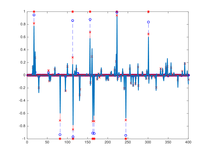
(a) True and Fitted signals. Red asterisks show true sparse signal; blue solid line shows LS estimate; solid dashed line ending in ‘x’ shows Huber estimate; thin dashed line ending with ‘o’ marker shows quantile Huber estimate.

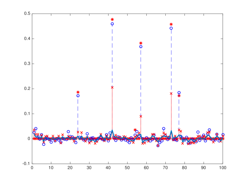
(b) True and Fitted Residuals. Red asterisk shows true outliers; blue solid line shows LS residual; solid dashed line ending in ‘x’ shows Huber residual; thin dashed line ending with ‘o’ marker shows quantile Huber residual.

Figure 4: Robust Asymmetric Recovery, comparing 2-norm, Huber, and quantile Huber penalties. $\kappa=0.1$ for both Huber penalties; quantile Huber has $\tau=0.9$ to capture the fact that outliers are expected to be positive.

5 Case studies

5.1 Low-rank matrix completion

A range of useful applications can be modeled as matrix completion problems. Important examples include applications in recommender systems and system identification (Recht, Fazel, Parillo [58]). The general principle extends to robust principal component analysis (RPCA), where we decompose a signal into low rank and sparse components, and its variants, including its stable version, which allows for noisy measurements. Applications include alignment of occluded images [57], scene triangulation [72], model selection [21], face recognition, and document indexing [19].

These problems can be formulated generally as

$$\mathop{\hbox{minimize}}_{X\in\mathbb{R}^{m\times n}}\quad\varphi(X)\quad\mathop{\hbox{subject to}}\quad\rho({\mathcal{A}}X-b)\leq\sigma,$$ (5.1)

where $b$ is a vector of observations, the linear operator ${\mathcal{A}}$ encodes information about the measurement process, and the objective $\varphi$ encourages the required structure in the solution, e.g., low-rank. The function $\rho$ measures the misfit between the linear model ${\mathcal{A}}X$ and the observations $b$. If we wish to require ${\mathcal{A}}X=b$, we can simply set $\sigma=0$ and choose any nonnegative convex function $\rho$ with $\rho^{-1}(0)=\{0\}$, e.g., $\rho=\left|\left|\cdot\right|\right|_{2}$. We categorize the problems of interest into two broad classes: symmetric and asymmetric problems. For each case, we outline how the level-set approach leads to implementable algorithms with computational kernels that scale gracefully with problem size.

The first class of problems aims to recover a low-rank PSD matrix, and in that case, the linear operator ${\mathcal{A}}$ maps between the space of symmetric $n\times n$ matrices and vectors, and we define the objective $\varphi$ by

$$\varphi_{1}(X)=\mathrm{tr}\,(X)+\delta_{\mathcal{S}^{n}_{+}}(X).$$

Problem (5.1) then reduces to finding a minimum-trace, PSD matrix that satisfies the measurements specified by ${\mathcal{A}}X=b$. There are analogs for optimization over complex Hermitian matrices; we focus on the real case only for simplicity. The formulation above captures, for example, the PhaseLift approach to the phase-retrieval problem, which aims to recover phase information about a signal (e.g., an image) by using only a series of magnitude measurements [20]. Important applications include optical wavefront reconstruction for astrophysical imaging [49] and the imaging of the molecular structure of a crystal via X-ray crystallography, which gives rise to such magnitude-only measurements; see Waldspurger, d’Aspremont, and Mallat [67] for a more complete description, including a number of other applications.

The second class of matrix-recovery problems does not require definiteness of $X$. In this case, the linear operator ${\mathcal{A}}$ on $\mathbb{R}^{m\times n}$ is not restricted to symmetric matrices, and we define $\varphi$ as the nuclear norm:

$$\varphi_{2}(X)=\left|\left|X\right|\right|_{*}:=\sum_{i=1}^{\mathclap{\min\{m,n\}}}\sigma_{i}(X),$$

where $\sigma_{i}(X)$ is the $i$th singular value of $X$. This formulation captures, for example, the bi-convex compressed sensing problem [48].

Example 5.1 (Robust PCA).

The second class captures a range of problems that are not immediately of the form (5.1). For example, the stable version of the RPCA problem [70] aims to decompose a matrix $Y$ as a sum of a low-rank matrix and a sparse matrix via the problem

$$\mathop{\hbox{minimize}}_{L,S}\quad\lambda\|L\|_{*}+\kappa\|S\|_{1}+\tfrac{1}{2}\|\mathcal{A}(L-Y)-S\|_{F}^{2}.$$ (5.2)

Here the operator $\mathcal{A}$ is often a mask for the known elements of $Y$. The goal is to obtain a low-rank approximation to $Y$ where the deviation from the known elements of $Y$ is as sparse as possible. The parameters $\lambda$ and $\kappa$ are are chosen to balance the rank of $L$ against the sparsity of the residual $S$ while minimizing the least-squared misfit. This model can be given a statistical interpretation that fits nicely into the context of robust regression as presented in Section 4.3.

We proceed by eliminating $S$ in (5.2) by first minimizing the objective over $S$ alone—an overlooked algorithmic technique for this problem. Observe that, as a function of $S$, the objective is the Moreau envelope of the 1-norm evaluated at ${\mathcal{A}}(L-Y)$, or, equivalently, the Huber function $\rho_{\kappa}$ on $\mathbb{R}^{m\times n}$ (4.14):

$$\inf_{S}\left\{\kappa\|S\|_{1}\!+\tfrac{1}{2}\|\mathcal{A}(L-Y)\!-\!S\|_{F}^{2}\right\}=\!\rho_{\kappa}(\mathcal{A}(L\!-\!Y)).$$

Problem (5.2) can now be written in terms of $L$ alone:

$$\mathop{\hbox{minimize}}_{L}\quad\lambda\|L\|_{*}+\rho_{\kappa}(\mathcal{A}(L-Y)).$$

This is the Lagrangian form of the robust estimation problem (4.15). Arguably, we can now interpret the goal of this problem as one of finding the lowest rank approximation to $Y$ over its known elements subject to a bound on a robust measure of misfit. This yields the problem

$$\mathop{\hbox{minimize}}_{L}\quad\left|\left|L\right|\right|_{*}\quad\mathop{\hbox{subject to}}\quad\rho_{\kappa}(\mathcal{A}(L-Y))\leq\sigma,$$ (5.3)

for some choice of parameter $\sigma\geq 0$. Various principled choices for $\sigma$ are discussed in §4.3.

Level-set approach and the Frank-Wolfe oracle

We apply the level-set approach, and exchange the roles of the regularizing function $\varphi$ and the misfit $\rho({\mathcal{A}}X-b)$. Note that the objective function $\varphi_{1}$ for the symmetric case vanishes at the origin, and is convex and positively homogeneous It is thus a gauge. The second objective function $\varphi_{2}$ is simply a norm. Therefore, for both cases, we may use the first row of Table 2 to determine the corresponding level-set subproblem and affine minorants based on dual certificates. In particular, the corresponding level-set subproblem $\mathcal{Q}_{\tau}$, which defines the value function, is

$$v(\tau):=\min_{X}\left\{\rho({\mathcal{A}}X-b)\,\left|\ \varphi(X)\leq\tau\right.\right\}.$$

We use the polar calculus described by Friedlander et al. [30, §7.2.1] and the definition of the dual norm to obtain the required polar functions

$$\varphi_{1}^{\circ}(Y)=\max\{0,\ \lambda_{1}(Y)\}\hbox{\qquad and\qquad}\varphi_{2}^{\circ}(Y)=\sigma_{1}(Y)$$

for the symmetric and asymmetric cases, respectively.

The evaluation of the affine minorant oracle requires an approximate solution of the optimization problem that defines the value function $v$, and computation of either an extreme eigenvalue or singular value to determine an affine minorant. As numerous authors have observed, the Frank-Wolfe algorithm [35, 29] is therefore especially well suited for evaluating the required quantities, and here we describe how to apply the algorithm to this setting.

The Frank-Wolfe subproblem (2.3), used to generate search directions at each iteration, takes the form

$$\mathop{\hbox{maximize}}_{S}\ \left\langle G,\,S\right\rangle\quad\mathop{\hbox{subject to}}\quad\varphi(S)\leq\tau.$$ (5.4)

where $G:={\mathcal{A}}^{*}\nabla\rho({\mathcal{A}}X-b)$ is the gradient of $\rho({\mathcal{A}}X-b)$ evaluated at the current primal iterate $X$. Note that the steplength in this case is easily obtained as the minimizer of the quadratic objective along the intersection of $[\varphi\leq\tau]$ and the ray $X+\mathbb{R}_{+}(S-X)$.

Solutions for the linearized subproblems can be obtained by computing extreme eigenvalues or singular values of $G$ [35, §4.2]. For the symmetric case, the constraint

$$\varphi_{1}(S)\leq\tau\hbox{\qquad is equivalent to\qquad}\mathrm{tr}\,(S)\leq\tau,\ S\succeq 0.$$

The linearized subproblem (5.4) is then solved by any matrix of the form

$$S=U\mbox{\rm Diag}\,(\xi_{i})U^{T}\quad\hbox{with}\quad\sum_{i=1}^{k}\xi_{i}=\tau,\ \xi_{i}\geq 0,$$

where $U\in\mathbb{R}^{n\times k}$ is the matrix that collects the $k$ eigenvectors of $G$ corresponding to $\lambda_{1}(G)$. For the non-symmetric case, the constraint $\varphi_{2}(S)\leq\tau$ is simply $\left|\left|S\right|\right|_{*}\leq\tau$, and the linearized subproblem is solved by any matrix of the form

$$S=U\mbox{\rm Diag}\,(\xi_{i})V^{T}\hbox{\qquad with\qquad}\sum_{i=1}^{k}\xi_{i}=\tau,\ \xi_{i}\geq 0,$$

where $U\in\mathbb{R}^{m\times k}$ and $V\in\mathbb{R}^{n\times k}$ are the matrices that collect the $k$ singular vectors of $G$ corresponding to the leading singular value $\sigma_{1}(G)$. In both cases, Krylov-based eigensolvers, such as ARPACK [42] can be used for the required eigenvalue and singular-value computation. If matrix-vector products with the matrix $\mathcal{A}^{*}y$ and its adjoint are computationally inexpensive, the computation of a few rightmost eigenvalue/eigenvector pairs (resp., maximum singular value/vector pairs) is much cheaper than the computation of the entire spectrum, as required by a method based on projections onto the feasible region. Such circumstances are common, for example when the operator $\mathcal{A}$ is sparse or it is accessible through a Fast Fourier Transform (FFT). The following example illustrates exactly this scenario.

Example 5.2 (Euclidean distance completion).

A common problem in distance geometry is the inverse problem: given only local pairwise Euclidean distance measurements among a set of points, recover their location in space. Formally, given a weighted undirected graph $G=(V,E,\omega)$ with a vertex set $V=\{1,\ldots,n\}$, and a target dimension $r$, the Euclidean distance completion problem asks to determine a collection of points $p_{1},\ldots,p_{n}$ in $\mathbb{R}^{r}$ approximately satisfying

$$\|p_{i}-p_{j}\|^{2}=\omega_{ij}\hbox{\qquad for all edges\qquad}ij\in E.$$

In literature, this problem is also often called $\ell_{2}$ graph embedding and appears in wireless networks, statics, robotics, protein reconstruction, and manifold learning; see the recent survey [46].

A popular convex relaxation for this problem was introduced by Weinberger et al. [68], and extensively studied by a number of authors [10, 12, 24]:

$$\begin{array}[]{ll}\mathop{\hbox{maximize}}&\mathrm{tr}\,X\\ \mathop{\hbox{subject to}}&\begin{aligned} &\|\mathcal{P}_{E}\circ\mathcal{K}(X)-\omega\|\leq\sigma,\\ &Xe=0,\ X\succeq 0,\end{aligned}\end{array}$$ (5.5)

where $\mathcal{K}\colon\mathcal{S}^{n}\to\mathcal{S}^{n}$ is the mapping $[\mathcal{K}(X)]_{ij}=X_{ii}+X_{jj}-2X_{ij}$ and $\mathcal{P}_{E}(D)$ is the canonical projection of a matrix $D$ onto entries indexed by the edge set $E$. Indeed, if $X$ is a rank $r$ feasible matrix, we may factor it into $X=PP^{T}$, where $P$ is an $n\times r$ matrix. It is then easy to see that the rows of $P$ are the points $p_{1},\ldots,p_{n}\in\mathbb{R}^{r}$ we seek. The constraint $Xe=0$ simply ensures that the points $p_{i}$ are centered around the origin. Notice, that this formulation directly contrasts the usual min-trace regularizer in compressed sensing; nonetheless, it is very natural. An easy computation shows that in terms of any factorization $X=PP^{T}$, the equality $\mathrm{tr}\,(X)=\frac{1}{2n}\sum^{n}_{i,j=1}\|p_{i}-p_{j}\|^{2}$ holds. Thus trace maximization serves to “flatten” the realization of the graph.

It is known that for $\sigma=0$, the problem formulation (5.5) notoriously fails strict feasibility [24, 25, 41]. In particular, for small $\sigma\geq 0$ the feasible region is very thin and the solution to the problem is unstable. As a result, algorithms maintaining feasibility are likely to exhibit some difficulties. In contrast, following the theme of this paper, we employ an infeasible method, and hence the poor conditioning of the underlying problem does not play a major role. The least-squares level-set problem that corresponds to the minimization formulation of (5.5) is

$$\begin{array}[t]{ll}\mathop{\hbox{minimize}}&\|\mathcal{P}_{E}\circ\mathcal{K}(X)-\omega\|\\ \mathop{\hbox{subject to}}&\mathrm{tr}\,X\geq\tau,\ Xe=0,\ X\succeq 0.\end{array}$$ (5.6)

Note the direction of the inequality $\mathrm{tr}\,X\geq\tau$, which takes into account that the original formulation (5.5) is a maximization problem. As a result, the root-finding method on the value function will approach the optimal value $\tau_{*}=\hbox{OPT}$ from the right. In particular, to initialize the approximate Newton scheme, we need an upper bound $\tau_{0}$ on the objective function. Such upper bounds are easily available from the diameter of the graph. See Figure 5 for an illustration.

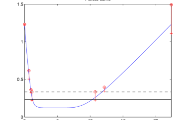
Figure 5: The value function $v(\tau):=\inf\left\{\|\mathcal{P}_{E}\circ\mathcal{K}(X)-\omega\|\,\left|\ \mathrm{tr}\,X=\tau,\ Xe=0,\ X\succeq 0\right.\right\}$. Newton’s method converges to either the minimum- or maximum-trace solution, depending on if it is started with an iterate to the left of the minimal root, or to the right of the maximal root. For a solution of (5.5), we require the maximal root. In this experiment, $\sigma=0.25$.

Note that the gradient of the objective function is typically very sparse (as sparse as the edge set $E$). Moreover, the linear subproblem over the feasible region is analogous to the ones considered in Section 5.1, requiring only a maximal eigenvalue computation on a sparse matrix (the gradient of the objective function); for more details see [24]. This makes the problem (5.6) ideally suited for the Frank-Wolfe algorithm, as discussed in §5.1. We note that the dual problem of (5.6) takes the form

$$\mathop{\hbox{maximize}}_{y\in\mathbb{R}^{E},\ \|y\|_{2}\leq 1}\quad\langle y,\omega\rangle-2\tau\lambda^{e^{\perp}}_{\max}(\mbox{\rm Diag}\,(Ye)-Y).$$

The matrix $Y=\mathcal{P}^{*}_{E}(y)$ is the vector $y$ padded with zeros and then $2(\mbox{\rm Diag}\,(Ye)-Y)=\mathcal{K}^{*}\mathcal{P}^{*}_{E}(y)$. The symbol $\lambda^{e^{\perp}}_{\max}(A)$ is the maximal eigenvalue of the restriction of the matrix $A$ to $e^{\perp}$. Hence, affine minorants are immediate to read off from the dual certificates generated by the Frank-Wolfe algorithm. An extensive numerical investigation of this approach is made by Drusvyatskiy et al. [24].

5.2 Robust elastic net regularization

In this final section, we explore an important data fitting problem where the regularizer $\varphi$ is not a gauge, unlike our previous examples. Zou and Hastie [73] introduced the elastic net regularizer

$$\varphi_{en}(x):=\alpha\|x\|_{1}+\frac{1-\alpha}{2}\|x\|_{2}^{2}\qquad(0\leq\alpha\leq 1)$$

for situations where there are multiple groups of covariates that are strongly correlated within each group. In this setting, the LASSO typically picks one member from each of the most important groups whereas the elastic net can pick out both the important groups and their members. As is the case with the Huber function, $\varphi_{en}$ is a member of the PLQ family [2, 3].

Zou and Hastie only consider the LS_τ and QP_λ formulations of the 1-norm regularized problem discussed in §1, but with $\|\cdot\|_{1}$ replaced by $\varphi_{en}$. Furthermore, they focus on the Lagrangian formulation QP_λ for computational reasons. The problem corresponding to BP_σ is not investigated. In this section, we provide a guide to the implementation of the methods of §2 for this version of the elastic net problem, but generalized to the case where the residual term is replaced by the Huber function $\rho_{\kappa}$ in (4.14) for robust inference. This gives the three formulations described in Table 5, which we call the robust elastic net problem.

$\mathcal{P}_{\sigma}$	$\mathcal{Q}_{\tau}$	Dual of $\mathcal{Q}_{\tau}$
$\begin{array}[t]{@{}c@{\ }l}\displaystyle\min_{x}&\varphi_{en}(x)\\ \textrm{s.t.}&\rho_{\kappa}({Ax-b})\leq\sigma\end{array}$	$\begin{array}[t]{c@{\;}l}\displaystyle\min_{x}&\rho_{\kappa}(Ax-b)\\ \textrm{s.t.}&\varphi_{en}(x)\leq\tau\end{array}$	$\begin{array}[t]{c@{\;}l@{}}\displaystyle\max_{y\in\kappa\mathbb{B}_{\infty}}&\left\langle b,\,y\right\rangle-\frac{\kappa}{2}\|y\|_{2}^{2}\ -\delta^{\star}_{[\varphi_{en}\leq\tau]}(A^{T}y)\end{array}$

Table 5: Elastic net

Inexact oracle for the value function

From Table 5, we determine the value function

$$v(\tau):=\min\left\{\rho_{\kappa}(Ax-b)\,\left|\ \varphi_{en}(x)\leq\tau\right.\right\}$$

to which we apply the root-finding procedure. We solve $\mathcal{Q}_{\tau}$ via an optimal gradient-projection algorithm, as described in §4.1.1. The methods require at each iteration a projection onto the level sets $[\varphi_{en}\leq\tau]$, which is given as the solution of the problem

$$\mathop{\hbox{minimize}}_{x}\quad\tfrac{1}{2}\|x-z\|_{2}^{2}\quad\mathop{\hbox{subject to}}\quad\varphi_{en}(x)\leq\tau.$$ (5.7)

The projection problem can be solved as follows. Assume without loss of generality $z\notin[\varphi_{en}\leq\tau]$ since otherwise $x:=z$ solves (5.7). We may also assume—possibly after a coordinate sign change—that $z\geq 0$. Observe then that any optimal solution $x$ satisfies $x\geq 0$. Thus, a feasible point $x$ solves (5.7) if and only if there exists a scalar $\lambda>0$ that satisfies

$$0\in(x-z)+\lambda(1-\alpha)x+\lambda\alpha\partial\|\cdot\|_{1}(x).$$

Equivalently,

$$z\in(1+\lambda(1-\alpha))x+\lambda\alpha\partial\|\cdot\|_{1}(x),$$

which amounts to the coordinate-wise inclusion

$$z_{i}\in(1+\lambda(1-\alpha))x_{i}+\lambda\alpha\partial|\cdot|(x_{i})\quad\mbox{for each $i=1,\dots,n$}.$$

In the case $x_{i}=0$, simple arithmetic shows $(z_{i}-\lambda\alpha\mathsf{sgn}{(z_{i})})_{+}=0$. Otherwise when $x_{i}\neq 0$, the numbers $x_{i}$ and $z_{i}$ are both strictly positive, and

$$x_{i}=\frac{(z_{i}-\lambda\alpha\mathsf{sgn}{(z_{i})})_{+}}{1+\lambda(1-\alpha)}=\frac{(z_{i}-\lambda\alpha)_{+}}{1+\lambda(1-\alpha)}.$$ (5.8)

Hence, regardless of whether $x_{i}$ is zero or not, (5.8) holds for all $i=1,\dots,n$. Plugging this into the relation $\varphi_{en}(x)=\tau$ gives

$$\tau =\alpha\sum_{i}\frac{(z_{i}-\lambda\alpha)_{+}}{1+\lambda(1-\alpha)}+\frac{(1-\alpha)}{2}\sum_{i}\frac{(z_{i}-\lambda\alpha)_{+}^{2}}{(1+\lambda(1-\alpha))^{2}}$$ (5.9)

$$=\frac{\alpha}{1+\lambda(1-\alpha)}\sum_{i}(z_{i}-\lambda\alpha)_{+}+\frac{(1-\alpha)}{2(1+\lambda(1-\alpha))^{2}}\sum_{i}(z_{i}-\lambda\alpha)_{+}^{2}.$$

The strong convexity of the objective in $x$ implies that there is a unique positive $\lambda$ that solves this equation. In addition, for $\lambda\geq\alpha^{-1}\|z\|_{\infty}$, the right-hand side of (5.9) is zero, while for $\lambda=0$, the right-hand side is $\varphi(z)>\tau$. So the unique optimal $\lambda$ resides in the open interval $(0,\alpha^{-1}\|z\|_{\infty})$. Finally, since $(1+\lambda(1-\alpha))>0$ for all $\lambda\geq 0$, equation (5.9) is equivalent to

$$0=\tau(1+\lambda(1-\alpha))^{2}-\alpha(1+\lambda(1-\alpha))\sum_{i}(z_{i}-\lambda\alpha)_{+}-\frac{(1-\alpha)}{2}\sum_{i}(z_{i}-\lambda\alpha)_{+}^{2}.$$

The root $\lambda$ is found by sorting coordinates of $z$ and then solving a quadratic polynomial in $\lambda$. Substituting $\lambda$ back into (5.8), we find the optimal $x$.

Affine minorant oracle for the value function

Following the approach of §2.3, for each candidate value of $\tau$ in Algorithm 2, we generate a dual certificate $y$ that yields a lower-bound on the value function $v(\tau)$. Such dual iterates are generated automatically by fast gradient methods on the primal problem [63]. To obtain an affine minorant of $v$, we then need a method for evaluating the function

$$\Phi(y,\tau):=\left\langle b,\,y\right\rangle-\tfrac{1}{2}\|y\|_{2}^{2}-\delta^{\star}_{[\varphi_{en}\leq\tau]}(A^{T}y),$$

and a subgradient $s\in\partial_{\tau}\delta^{\star}_{[\varphi_{en}\leq\tau]}(A^{T}y)$. To this end, we use the representation

$$\delta^{\star}_{[\varphi_{en}\leq\tau]}(z)=\inf_{\mu>0}[\tau\mu+\mu\varphi_{en}^{\star}(\mu^{-1}z)].$$

See, for example, Aravkin et al. [3, Equation 6.5c]. Since $\varphi_{en}$ is the sum of two finite-valued convex functions, its conjugate is the infimal convolution

$$\varphi_{en}^{\star}(z)=\inf_{v\in\alpha\mathbb{B}_{\infty}}\frac{1}{2(1-\alpha)}\|z-v\|_{2}^{2}=\frac{1}{2(1-\alpha)}\hbox{dist}^{2}_{\alpha\mathbb{B}_{\infty}}(z)=\frac{1}{2(1-\alpha)}\|(\left|z\right|-\alpha e)_{+}\|_{2}^{2}.$$

Hence, for $\mu>0$, we have

$$\delta^{\star}_{[\varphi_{en}\leq\tau]}(z)=\inf_{\mu>0}~{}\left\{\tau\mu+\frac{1}{2(1-\alpha)\mu}\|(\left|z\right|-\mu\alpha\mathrm{e})_{+}\|_{2}^{2}\right\},$$ (5.10)

and the derivative of $\delta^{\star}_{[\varphi_{en}\leq\tau]}(z)$ with respect to $\tau$ is given by the optimal $\mu$ when it exists. Note that if $\mu\geq\alpha^{-1}\|z\|_{\infty}$, then $[\tau\mu+\frac{1}{2(1-\alpha)\mu}\|(\left|z\right|-\mu\alpha\mathrm{e})_{+}\|_{2}^{2}]=\tau\mu$, while for $\mu\to 0$ we have $[\tau\mu+\frac{1}{2(1-\alpha)\mu}\|(\left|z\right|-\alpha\mu\mathrm{e})_{+}\|_{2}^{2}]\to+\infty$. Hence, an optimal $\mu$ exists when $\tau>0$. It is also unique due to the convex piecewise quadratic nature of the objective. Consequently, the optimal $\mu$ in (5.10) can be obtained by sorting $|z|$ and then writing in closed form the solution of a sequence of elementary univariate convex functions over an interval.

Appendix A Proofs

Theorem A.1 (Superlinear convergence of Newton and secant methods).

Let $f\colon\mathbb{R}^{n}\to\mathbb{R}$ be a non-increasing, convex function on the interval $[a,b]$. Suppose that the point $\tau_{*}:=\inf\{\tau:f(\tau)\leq 0\}$ lies in $(a,b)$ and the non-degeneracy condition $g_{*}:=\inf\left\{g\,\left|\ g\in\partial f(\tau_{*})\right.\right\}<0$ holds. Fix two points $\tau_{-1},\tau_{1}\in(a,b)$ satisfying $\tau_{0}<\tau_{1}<\tau_{*}$ and consider the following two iterations:

$$\tau_{k+1}:=\begin{cases}\tau_{k}&\mbox{if $f(\tau_{k})=0$,}\\ \tau_{k}-\frac{f(\tau_{k})}{g_{k}}\qquad\mbox{[for $g_{k}\in\partial f(\tau_{k})$]}&\mbox{otherwise;}\end{cases}$$ (Newton)

and

$$\tau_{k+1}:=\begin{cases}\tau_{k}&\mbox{if $f(\tau_{k})=0$,}\\ \tau_{k}-\frac{\tau_{k}-\tau_{k-1}}{f(\tau_{k})-f(\tau_{k-1})}f(\tau_{k})&\mbox{otherwise.}\end{cases}\quad$$ (Secant)

If either sequence terminates finitely at some $\tau_{k}$, then it must be the case $\tau_{k}=\tau_{*}$. If the sequence $\{\tau_{k}\}$ does not terminate finitely, then $|\tau_{*}-\tau_{k+1}|\leq(1-\frac{g_{*}}{\gamma_{k}})|\tau_{*}-\tau_{k}|,\ k=1,2,\dots$, where $\gamma_{k}=g_{k}$ for the Newton sequence and $\gamma_{k}$ is any element of $\partial f(\tau_{k-1})$ for the secant sequence. In either case, $\gamma_{k}\uparrow g_{*}$ and $\tau_{k}\uparrow\tau_{*}$ globally $q$-superlinearly.

Proof.

Since $f$ is convex, the subdifferential $\partial f(\tau)$ is nonempty for all $\tau\in(a,b)$. The claim concerning finite termination is easy to deduce from convexity; we leave the details to the reader. Suppose neither sequence terminates finitely at $\tau_{*}$. Let us first consider the Newton iteration. Convexity of $f$ immediately implies that the sequence $\tau_{i}$ is well-defined and satisfies $\tau_{0}<\tau_{1}<\tau_{2}<\dots<\tau_{*}$. Monotonicity of the subdifferential then implies $g_{0}\leq g_{1}\leq g_{2}\leq\dots\leq g_{*}<0$. Due to the inequalities $f(\tau_{*})+\bar{g}(\tau_{k}-\tau_{*})\leq f(\tau_{k})$ and $g_{k}<0$, we have

$$\frac{f(\tau_{k})-f(\tau_{*})}{g_{k}}\leq-\frac{g_{*}}{g_{k}}(\tau_{*}-\tau_{k}),$$

and so

$$0<\tau_{*}-\tau_{k+1}=\tau_{*}-\tau_{k}+\frac{f(\tau_{k})-f(\tau_{*})}{g_{k}}\leq\left(1-\frac{g_{*}}{g_{k}}\right)(\tau_{*}-\tau_{k}).$$

Upper semi-continuity of $\partial f$ on its domain implies $g_{k}\uparrow g_{*}$. Hence $\tau_{k}$ converge $q$-superlinearly to $\tau_{*}$.

Now consider the secant iteration. As in the Newton iteration, it is immediate from convexity that the sequence $\tau_{i}$ is well-defined and satisfies $\tau_{0}<\tau_{1}<\tau_{2}<\dots<\tau_{*}$. Monotonicity of the subdifferential then implies $g_{0}\leq g_{1}\leq g_{2}\leq\dots\leq g_{*}<0$. We have

$$0<g_{*}(\tau_{k}-\tau_{*})\leq f(\tau_{k})-f(\tau_{*}),$$

and $f(\tau_{k-1})+g_{k-1}(\tau_{k}-\tau_{k-1})\leq f(\tau_{k})$, and hence

$$\frac{\tau_{k}-\tau_{k-1}}{f(\tau_{k})-f(\tau_{k-1})}(f(\tau_{k})-f(\tau_{*}))\leq\frac{f(\tau_{k})-f(\tau_{*})}{g_{k-1}}<0.$$

Combining the two inequalities yields

$$\frac{f(\tau_{k})-f(\tau_{*})}{f(\tau_{k})-f(\tau_{k-1})}(\tau_{k}-\tau_{k-1})\leq\frac{f(\tau_{k})-f(\tau_{*})}{g_{k-1}}\leq\frac{g_{*}}{g_{k-1}}(\tau_{k}-\tau_{*})<0.$$

Consequently, we deduce

$$0<\tau_{*}-\tau_{k+1}=\tau_{*}-\tau_{k}+\frac{f(\tau_{k})-f(\tau_{*})}{f(\tau_{k})-f(\tau_{k-1})}(\tau_{k}-\tau_{k-1})\leq\left(1-\frac{g_{*}}{g_{k-1}}\right)(\tau_{*}-\tau_{k}).$$

The result follows. ∎

Proof of Theorem 2.2.

It is easy to see by convexity that the iterates $\tau_{k}$ are strictly increasing and satisfy $f(\tau_{k})>0$. For each index $j\geq 2$, define the following quantities:

$$h_{j}:=\tau_{j}-\tau_{j-1},\quad\quad\theta_{j}:=\frac{s_{j}}{s_{j-1}},\quad\textrm{ and }\quad\gamma_{j}:=\frac{\ell_{j}}{\ell_{j-1}}.$$

Note that using the equation $\tau_{j-1}-\tau_{j}=\frac{\ell_{j-1}}{s_{j-1}}$, we can write $\theta_{j}=\frac{u_{j-1}-\ell_{j}}{\ell_{j-1}}$. Clearly then the bound, $0\leq\theta_{j}\leq\alpha-\gamma_{j}$, is valid. Define now constants $\beta_{j}\in[0,1]$ by the equation $\gamma_{j}=\beta_{j}\alpha$. Suppose $k\geq 2$ is an index at which the algorithm has not terminated, i.e., $u_{k}>\epsilon$. Taking into account the inequality $\ell_{k}\geq\frac{u_{k}}{\alpha}>\frac{\epsilon}{\alpha}$, we deduce

$$\frac{\epsilon}{\alpha}\leq\ell_{k}=\ell_{1}\prod_{j=2}^{k}\gamma_{j}\leq C\alpha^{k-1}\prod_{j=2}^{k}\beta_{j}.\$$ (A.1)

The defining equation for $\tau_{k+1}$ and the definition of $\theta_{j}$ yield the equality

$$h_{k+1}=\frac{\ell_{k}}{|s_{k}|}=\frac{\ell_{k}}{|s_{1}|}\cdot\prod_{j=2}^{k}\theta_{j}^{-1}.$$

The bounds $\tau_{*}-\tau_{1}\geq h_{k+1}$, $\ell_{k}\geq\frac{\epsilon}{\alpha}$, and $\theta_{j}\leq\alpha-\gamma_{j}$ imply

$$\tau_{*}-\tau_{1}\geq\frac{\ell_{k}}{|s_{1}|}\cdot\prod_{j=2}^{k}\theta_{j}^{-1}\geq\frac{\epsilon}{\alpha|s_{1}|}(\alpha^{-1})^{k-1}\prod_{j=2}^{k}(1-\beta_{j})^{-1},$$

and rearranging gives

$$\epsilon\leq(\tau_{*}-\tau_{1})|s_{1}|\alpha^{k}\prod_{j=2}^{k}(1-\beta_{j})\leq C\alpha^{k}\prod_{j=2}^{k}(1-\beta_{j}).$$ (A.2)

Combining (A.1) and (A.2), we get

$$\epsilon\leq C\alpha^{k}\min\left\{\prod_{j=2}^{k}\beta_{j},\ \prod_{j=2}^{k}(1-\beta_{j})\right\}.$$ (A.3)

One the other hand, observe

$$\left(\prod_{j=2}^{k}\beta_{j}\right)\left(\prod_{j=2}^{k}(1-\beta_{j})\right)=\prod_{j=2}^{k}\beta_{j}(1-\beta_{j})\leq 0.5^{2(k-1)},$$

and hence

$$\min\left\{\prod_{j=2}^{k}\beta_{j},\ \prod_{j=2}^{k}(1-\beta_{j})\right\}\leq 0.5^{k-1}.$$ (A.4)

Combining equations (A.4) and (A.3), the claimed estimate $k-1\leq\log_{2/\alpha}\left(\frac{\alpha C}{\epsilon}\right)$ follows. ∎

Proof of Theorem 2.4.

The proof is identical to the proof of Theorem 2.2, except for some minor modifications. The only nontrivial change is how we arrive at the bound $\theta_{j}\leq\alpha-\gamma_{j}$. For this, observe $\tau_{j-1}-\tau_{j}=\ell_{j-1}/s_{j-1}$, and because the function $\tau\mapsto\ell_{j}+s_{j}(\tau-\tau_{j})$ minorizes $v$, we see

$$u_{j-1} \geq\ell_{j}+s_{j}(\tau_{j-1}-\tau_{j})=\ell_{j}+s_{j}\left(\frac{\ell_{j-1}}{s_{j-1}}\right)=\ell_{j}+\theta_{j}\ell_{j-1}.$$

After rearranging, we get the desired upper bound on $\theta_{j}$:

$$\theta_{j} \leq\frac{u_{j-1}-\ell_{j}}{\ell_{j-1}}\leq\alpha-\gamma_{j}.$$

Finally, we remark that with the approximate Newton method, we can start indexing at $j=0$ instead of $j=1$. This explains the different constants in the convergence result. ∎

Lemma A.2 (Concavity of the parametric support function).

For any convex function $f\colon\mathbb{R}^{n}\to\overline{\mathbb{R}}$ and vector $z\in\mathbb{R}^{n}$, the univariate function $t\mapsto\delta^{*}_{[f\leq t]}(z)$ is concave.

Proof.

Convexity of $f$ immediately yields the inclusion

$$\lambda\cdot[f\leq a]+(1-\lambda)\cdot[f\leq b]\subseteq[f\leq\lambda a+(1-\lambda)b]\qquad\forall a,b\in\mathbb{R}\text{ and }\lambda\in[0,1].$$

We deduce $\lambda\cdot\delta^{*}_{[f\leq a]}(z)+(1-\lambda)\cdot\delta^{*}_{[f\leq b]}(z)=\delta^{*}_{\lambda\cdot[f\leq a]+(1-\lambda)\cdot[f\leq b]}(z)\leq\delta^{*}_{[f\leq\lambda a+(1-\lambda)b]}(z)$, and the result follows. ∎

Proof of Proposition 3.1.

For this proof only, let $\|\cdot\|$ denote the 2-norm. Note the inclusion $s/\|y\|\in\partial_{\tau}\Phi_{1}\left(y/\|y\|,\,\tau\right)$. Use the same computation from (2.2) to deduce that the affine function

$$\tau^{\prime}\mapsto(\hat{\ell}-\sigma)-\frac{s}{\|y\|}(\tau^{\prime}-\tau)$$

minorizes $f_{1}$.

From the definition of $\hat{\ell}$, $\Phi_{1}$, and $\Phi_{2}$, it follows that

$$\frac{u-\sigma}{\hat{\ell}-\sigma}=\frac{(u-\sigma)\|y\|}{\Phi_{2}(y,\tau)+\frac{1}{2}\|y\|^{2}-\sigma\|y\|}=\frac{2(u-\sigma)\|y\|}{\ell^{2}+\|y\|^{2}-2\sigma\|y\|}.$$ (A.5)

Taking into account the equivalence

$$\frac{u-\sigma}{\ell-\sigma}\leq\alpha\quad\iff\quad\frac{u+(\alpha-1)\sigma}{\alpha}\leq\ell,$$

we deduce

$$\ell^{2}+\|y\|^{2}-2\sigma\|y\|\geq\alpha^{-2}\Big{(}(u+(\alpha-1)\sigma)^{2}+\|\alpha y\|^{2}-2\sigma\alpha\|\alpha y\|\Big{)}\geq 2\alpha^{-1}(u-\sigma)\|y\|,$$

where the rightmost inequality follows from the computation

$$(u+[\alpha-1]\sigma)^{2} +\|\alpha y\|^{2}-2\alpha\sigma\|\alpha y\|-2(u-\sigma)\|\alpha y\|$$

$$=\left(u+[\alpha-1]\sigma\right)^{2}+\|\alpha y\|^{2}-2\|\alpha y\|(u+[\alpha-1]\sigma)$$

$$=\left(u+[\alpha-1]\sigma-\|\alpha y\|\right)^{2}\geq 0.$$

Because the right-hand side of (A.5) is non-negative, we can deduce that $\hat{\ell}\geq\sigma$. Finally, the required inequality $(u-\sigma)/(\hat{\ell}-\sigma)\leq\alpha$ also follows from (A.5). ∎

Lemma A.3.

$(-\lambda_{\min})^{\star}(y)=\delta_{\mathcal{S}}(-y)$, where $\mathcal{S}={\mathcal{K}}^{*}\cap\left\{x\mid\left\langle e,\,x\right\rangle=1\right\}$.

Proof.

The following formula is established in [60]:

$$\partial(-\lambda_{\min})(x)=\left\{-y\mid\left\langle y,\,e\right\rangle=1,\ \left\langle y,\,z-(x-\lambda_{\min}(x)e)\right\rangle\geq 0\text{ for all }z\in\mathcal{K}\right\}$$

or equivalently

$$\partial(-\lambda_{\min})(x) =\left\{-y\,\left|\ \left\langle y,\,e\right\rangle=1,-y\in N_{\mathcal{K}}\left(x-\lambda_{\min}(x)e\right)\right.\right\}$$

$$=\left\{-y\,\left|\ \left\langle y,\,e\right\rangle=1,\ y\in\mathcal{K}^{*},\ 0=\lambda_{\min}(x)-\left\langle y,\,x\right\rangle\right.\right\}.$$

Here the symbol $N_{\mathcal{K}}$ denotes the normal cone to $\mathcal{K}$. Now for any $y\in\partial(-\lambda_{\min})(x)$, we have $\langle x,y\rangle=-\lambda_{\min}(x)$. Observe $\mathrm{range}\,\partial(-\lambda_{\min})=-\mathcal{S}$. Hence by the equality in the Fenchel-Young inequality, for any $y\in-\mathcal{S}$, we have $(-\lambda_{\min})^{\star}(y)=0$. On the other hand, for any $y$ with $\langle y,e\rangle\neq-1$, we have $(-\lambda_{\min})^{\star}(y)\geq\langle te,y\rangle-(-\lambda_{\min})(te)=t(\langle y,e\rangle+1)$ for any $t\geq 0$. Letting $t\to\infty$, we deduce $(-\lambda_{\min})^{\star}(y)=+\infty$. Similarly, consider $y\notin-\mathcal{K}^{*}$. Then we may find some $x\in\mathcal{K}$ satisfying $\langle x,y\rangle>0$. We deduce $(-\lambda_{\min})^{\star}(y)\geq\langle tx,y\rangle-(-\lambda_{\min})(tx)=t(\langle y,x\rangle-(-\lambda_{\min})(x))$ for any $t\geq 0$. Letting $t\to\infty$, we deduce $(-\lambda_{\min})^{\star}(y)=+\infty$. We deduce that $(-\lambda_{\min})^{\star}$ is the indicator function of $-\mathcal{S}$, as claimed. ∎

Lemma A.4.

Let ${\mathcal{D}}_{1}$ and ${\mathcal{D}}_{2}$ be two nonempty closed convex sets that contain the origin. Then $\gamma_{{\mathcal{D}}_{1}}+\gamma_{{\mathcal{D}}_{2}}=\gamma_{({\mathcal{D}}_{1}^{\circ}+{\mathcal{D}}_{2}^{\circ})^{\circ}}$. If additionally $0\in\operatorname{int}{{\mathcal{D}}_{1}}$, then $(\gamma_{{\mathcal{D}}_{1}}+\gamma_{{\mathcal{D}}_{2}})^{\circ}=\gamma_{{\mathcal{D}}_{1}^{\circ}+{\mathcal{D}}_{2}^{\circ}}.$

Proof.

Theorem 14.5 of [61] contains most of the needed tools. In particular, the gauge of any closed convex function containing the origin is the support function of the polar. Thus,

$$\gamma_{{\mathcal{D}}_{1}}+\gamma_{{\mathcal{D}}_{2}}=\delta^{*}_{{\mathcal{D}}_{1}^{\circ}}+\delta^{*}_{{\mathcal{D}}_{2}^{\circ}}.$$

By [33, Cor. 3.2.5], we have

$$\delta^{*}_{{\mathcal{D}}_{1}^{\circ}}+\delta^{*}_{{\mathcal{D}}_{2}^{\circ}}=\delta^{*}_{\mathrm{cl}\left({\mathcal{D}}_{1}^{\circ}+{\mathcal{D}}_{2}^{\circ}\right)}=\delta^{*}_{{\mathcal{D}}_{1}^{\circ}+{\mathcal{D}}_{2}^{\circ}},$$

where the last equality holds because the support function does not distinguish a set from its closure. Again using the polarity correspondence between the gauge and support functions, we have $\gamma_{{\mathcal{D}}_{1}}+\gamma_{{\mathcal{D}}_{2}}=\gamma_{({\mathcal{D}}_{1}^{\circ}+{\mathcal{D}}_{2}^{\circ})^{\circ}}$, as required. We now prove the second part of the lemma. Use the first part of the result and [61, Thm. 15.1] to deduce that

$$(\gamma_{{\mathcal{D}}_{1}}+\gamma_{{\mathcal{D}}_{2}})^{\circ}=\gamma_{({\mathcal{D}}_{1}^{\circ}+{\mathcal{D}}_{2}^{\circ})^{\circ\circ}}.$$ (A.6)

Because $0\in\operatorname{int}{{\mathcal{D}}_{1}}$, the set ${\mathcal{D}}_{1}^{\circ}$ is compact [61, Cor. 14.5], and because ${\mathcal{D}}_{2}^{\circ}$ is closed, ${\mathcal{D}}_{1}^{\circ}+{\mathcal{D}}_{2}^{\circ}$ is also closed. Thus, $({\mathcal{D}}_{1}^{\circ}+{\mathcal{D}}_{2}^{\circ})^{\circ\circ}={\mathcal{D}}_{1}^{\circ}+{\mathcal{D}}_{2}^{\circ}$. It then follows from (A.6) that $(\gamma_{{\mathcal{D}}_{1}}+\gamma_{{\mathcal{D}}_{2}})^{\circ}=\gamma_{({\mathcal{D}}_{1}^{\circ}+{\mathcal{D}}_{2}^{\circ})}$, as required. ∎

Remark A.5 (Projection onto a conic slice sets).

This remark is standard. Fix a proper convex cone ${\mathcal{K}}$ and consider the projection problem

$$\min_{x}\ \left\{\tfrac{1}{2}\|x-z\|^{2}\,\left|\ \langle c,x\rangle=1,\,x\in\mathcal{K}\right.\right\}.$$

Equivalently, we can consider the univariate concave maximization problem

$$\max_{\beta}\min_{x\in{\mathcal{K}}}\,L(x,\beta) =\max_{\beta}\min_{x\in{\mathcal{K}}}\,\tfrac{1}{2}\|x-z\|^{2}+\beta(\langle c,x\rangle-1)$$

$$=\max_{\beta}\min_{x\in{\mathcal{K}}}\,\tfrac{1}{2}\|x-(z-\beta c)\|^{2}+\beta(\langle c,z\rangle-1)-\tfrac{1}{2}\beta^{2}\|c\|^{2}$$

$$=\max_{\beta}~{}\tfrac{1}{2}\hbox{dist}^{2}_{\mathcal{K}}(z-\beta c)+\beta(\langle c,z\rangle-1)-\tfrac{1}{2}\beta^{2}\|c\|^{2}.$$

We can solve this problem for example by bisection, provided projections onto ${\mathcal{K}}$ are available.

References

- A. Aravkin et al. [2014] A. Aravkin, P. Kambadur, A. Lozano, and R. Luss. Orthogonal matching pursuit for sparse quantile regression. In Data Mining (ICDM), International Conference on, pages 11–19. IEEE, 2014.
- Aravkin et al. [2013a] A. Aravkin, J. V. Burke, and G. Pillonetto. Sparse/robust estimation and kalman smoothing with nonsmooth log-concave densities: Modeling, computation, and theory. Journal of Machine Learning Research, 14:2689–2728, 2013a. URL http://jmlr.org/papers/v14/aravkin13a.html.
- Aravkin et al. [2013b] A. Y. Aravkin, J. Burke, and M. P. Friedlander. Variational properties of value functions. SIAM J. Optimization, 23(3):1689–1717, 2013b.
- Bach [2015] F. Bach. Duality between subgradient and conditional gradient methods. SIAM J. Optim., 25(1):115–129, 2015. ISSN 1052-6234. doi: 10.1137/130941961. URL http://dx.doi.org/10.1137/130941961.
- Beck and Teboulle [2003] A. Beck and M. Teboulle. Mirror descent and nonlinear projected subgradient methods for convex optimization. Operations Research Letters, 31(3):167–175, 2003.
- Ben-Tal and Nemirovski [2001] A. Ben-Tal and A. Nemirovski. Lectures on modern convex optimization. MPS/SIAM Series on Optimization. Society for Industrial and Applied Mathematics (SIAM), Philadelphia, PA; Mathematical Programming Society (MPS), Philadelphia, PA, 2001. ISBN 0-89871-491-5. doi: 10.1137/1.9780898718829. URL http://dx.doi.org/10.1137/1.9780898718829. Analysis, algorithms, and engineering applications.
- Bertsekas [2015] D. P. Bertsekas. Convex optimization algorithms. Athena Scientific, Massachusetts, 2015.
- Bioucas-Dias and Figueiredo [2010] J. M. Bioucas-Dias and M. A. Figueiredo. Alternating direction algorithms for constrained sparse regression: Application to hyperspectral unmixing. In Hyperspectral Image and Signal Processing: Evolution in Remote Sensing (WHISPERS), 2010 2nd Workshop on, pages 1–4. IEEE, 2010.
- Biswas and Ye [2004] P. Biswas and Y. Ye. Semidefinite programming for ad hoc wireless sensor network localization. In Proceedings of the 3rd international symposium on Information processing in sensor networks, pages 46–54. ACM, 2004.
- Biswas and Ye [2006] P. Biswas and Y. Ye. A distributed method for solving semidefinite programs arising from ad hoc wireless sensor network localization. In Multiscale optimization methods and applications, volume 82 of Nonconvex Optim. Appl., pages 69–84. Springer, New York, 2006. doi: 10.1007/0-387-29550-X˙2. URL http://dx.doi.org/10.1007/0-387-29550-X_2.
- Biswas et al. [2006a] P. Biswas, T.-C. Lian, T.-C. Wang, and Y. Ye. Semidefinite programming based algorithms for sensor network localization. ACM Transactions on Sensor Networks (TOSN), 2(2):188–220, 2006a.
- Biswas et al. [2006b] P. Biswas, T.-C. Liang, K.-C. Toh, Y. Ye, and T.-C. Wang. Semidefinite programming approaches for sensor network localization with noisy distance measurements. Automation Science and Engineering, IEEE Transactions on, 3(4):360–371, Oct 2006b. ISSN 1545-5955. doi: 10.1109/TASE.2006.877401.
- Borwein and Lewis [2000] J. Borwein and A. Lewis. Convex analysis and nonlinear optimization. CMS Books in Mathematics/Ouvrages de Mathématiques de la SMC, 3. Springer-Verlag, New York, 2000. ISBN 0-387-98940-4. Theory and examples.
- Boyd et al. [2011] S. Boyd, N. Parikh, E. Chu, B. Peleato, and J. Eckstein. Distributed optimization and statistical learning via the alternating direction method of multipliers. Foundations and Trends® in Machine Learning, 3(1):1–122, 2011.
- Brucker [1984] P. Brucker. An o(n) algorithm for quadratic knapsack problems. Operations Research Letters, 3(3):163 – 166, 1984. ISSN 0167-6377. doi: http://dx.doi.org/10.1016/0167-6377(84)90010-5. URL http://www.sciencedirect.com/science/article/pii/0167637784900105.
- Bube and Nemeth [2007] K. Bube and T. Nemeth. Fast line searches for the robust solution of linear systems in the hybrid and huber norms. Geophysics, 72(2):A13–A17, 2007.
- Buchinsky [1994] M. Buchinsky. Changes in the u.s. wage structure 1963-1987: Application of quantile regression. Econometrica, 62(2):405–58, March 1994.
- Candès and Tao [2010] E. Candès and T. Tao. The power of convex relaxation: Near-optimal matrix completion. IEEE Trans. Info. Th., 56(5):2053–2080, 2010.
- Candès et al. [2011] E. J. Candès, X. Li, Y. Ma, and J. Wright. Robust principal component analysis? J. Assoc. Comput. Mach., 58(3):1–37, May 2011.
- Candès et al. [2012] E. J. Candès, T. Strohmer, and V. Voroninski. Phaselift: Exact and stable signal recovery from magnitude measurements via convex programming. Commun. Pur. Appl. Ana., 2012.
- Chandrasekaran et al. [2012] V. Chandrasekaran, P. A. Parrilo, and A. S. Willsky. Latent variable graphical model selection via convex optimization. Ann. Stat., 40(4):1935–2357, 2012.
- Chen et al. [1999] S. S. Chen, D. L. Donoho, and M. A. Saunders. Atomic decomposition by basis pursuit. SIAM J. Sci. Comput., 20(1):33–61, 1999. ISSN 10648275. doi: 10.1137/S1064827596304010. URL http://link.aip.org/link/SJOCE3/v20/i1/p33/s1&Agg=doihttp://citeseerx.ist.psu.edu/viewdoc/download?doi=10.1.1.37.4272&rep=rep1&type=pdf.
- Clark [1985] D. I. Clark. The mathematical structure of huber’s m-estimator. SIAM journal on scientific and statistical computing, 6(1):209–219, 1985.
- Drusvyatskiy et al. [2014] D. Drusvyatskiy, N. Krislock, Y.-L. Voronin, and H. Wolkowicz. Noisy Euclidean distance realization: robust facial reduction and the Pareto frontier. Preprint, arXiv:1410.6852, 2014.
- Drusvyatskiy et al. [2015] D. Drusvyatskiy, G. Pataki, and H. Wolkowicz. Coordinate shadows of semidefinite and Euclidean distance matrices. SIAM J. Optim., 25(2):1160–1178, 2015. ISSN 1052-6234. doi: 10.1137/140968318. URL http://dx.doi.org/10.1137/140968318.
- Dutter and Huber [1981] R. Dutter and P. J. Huber. Numerical methods for the nonlinear robust regression problem. Journal of Statistical Computation and Simulation, 13:79–113, 1981.
- Ennis and McGuire [2001] R. h. Ennis and G. C. McGuire. Computer Algebra Recipes: A Gourmet’s Guide to the Mathematical Models of Science. Springer, 2001.
- Fazel [2002] M. Fazel. Matrix rank minimization with applications. PhD thesis, Elec. Eng. Dept, Stanford University, 2002.
- Frank and Wolfe [1956] M. Frank and P. Wolfe. An algorithm for quadratic programming. Naval Res. Logist. Quart., 3:95–110, 1956. ISSN 0028-1441.
- Friedlander et al. [2014] M. Friedlander, I. Macêdo, and T. Pong. Gauge optimization and duality. SIAM J. Optim., 24(4):1999–2022, 2014. doi: 10.1137/130940785.
- Gabay and Mercier [1976] D. Gabay and B. Mercier. A dual algorithm for the solution of nonlinear variational problems via finite element approximations. Computers and Mathematics with Applications, 2(1):17–40, 1976.
- Harchaoui et al. [2015] Z. Harchaoui, A. Juditsky, and A. Nemirovski. Conditional gradient algorithms for norm-regularized smooth convex optimization. Math. Program., 152(1-2, Ser. A):75–112, 2015. ISSN 0025-5610. doi: 10.1007/s10107-014-0778-9. URL http://dx.doi.org/10.1007/s10107-014-0778-9.
- Hiriart-Urruty and Lemaréchal [2001] J.-B. Hiriart-Urruty and C. Lemaréchal. Fundamentals of Convex Analysis. Springer, New York, NY, USA, 2001.
- Huber [2004] P. J. Huber. Robust Statistics. John Wiley and Sons, 2 edition, 2004.
- Jaggi [2013] M. Jaggi. Revisiting Frank-Wolfe: Projection-free sparse convex optimization. In Proc. 30th Intern. Conf. Machine Learning (ICML-13), pages 427–435, 2013.
- Kekatos and Giannakis [2011] V. Kekatos and G. B. Giannakis. From sparse signals to sparse residuals for robust sensing. Signal Processing, IEEE Transactions on, 59(7):3355–3368, 2011.
- Koenker [2005] R. Koenker. Quantile Regression. Cambridge University Press, 2005.
- Koenker and Bassett [1978] R. Koenker and G. Bassett. Regression quantiles. Econometrica, pages 33–50, 1978.
- Koenker and Geling [2001] R. Koenker and O. Geling. Reappraising medfly longevity: A quantile regression survival analysis. Journal of the American Statistical Association, 96:458–468, 2001.
- Koenker and Hallock [2001] R. Koenker and K. F. Hallock. Quantile regression. Journal of Economic Perspectives, American Economic Association, pages 143–156, 2001.
- Krislock and Wolkowicz [2010] N. Krislock and H. Wolkowicz. Explicit sensor network localization using semidefinite representations and facial reductions. SIAM J. Optim., 20(5):2679–2708, 2010. ISSN 1052-6234. doi: 10.1137/090759392. URL http://dx.doi.org.offcampus.lib.washington.edu/10.1137/090759392.
- Lehoucq et al. [1998] R. B. Lehoucq, D. C. Sorensen, and C. Yang. ARPACK Users’ guide: solution of large-scale eigenvalue problems with implicitly restarted Arnoldi methods, volume 6. SIAM, 1998.
- Lemaréchal [1975] C. Lemaréchal. An extension of Davidon methods to nondifferentiable problems. Math. Programming Stud., 3:95–109, 1975.
- Lemaréchal et al. [1995] C. Lemaréchal, A. Nemirovskii, and Y. Nesterov. New variants of bundle methods. Math. Programming, 69(1, Ser. B):111–147, 1995. ISSN 0025-5610. doi: 10.1007/BF01585555. URL http://dx.doi.org/10.1007/BF01585555. Nondifferentiable and large-scale optimization (Geneva, 1992).
- Li and Swetits [1998] W. Li and J. Swetits. The linear l1 estimator and the huber m-estimator. SIAM Journal on Optimization, 8(2):457–475, 1998.
- Liberti et al. [2014] L. Liberti, C. Lavor, N. Maculan, and A. Mucherino. Euclidean distance geometry and applications. SIAM Review, 56(1):3–69, 2014. doi: 10.1137/120875909. URL http://dx.doi.org/10.1137/120875909.
- Lichman [2013] M. Lichman. UCI machine learning repository, 2013. URL http://archive.ics.uci.edu/ml.
- Ling and Strohmer [2015] S. Ling and T. Strohmer. Self-calibration and biconvex compressive sensing. CoRR, abs/1501.06864, 2015. URL http://arxiv.org/abs/1501.06864.
- Luke et al. [2002] R. Luke, J. Burke, and R. Lyons. Optical wavefront reconstruction: theory and numerical methods. SIAM Review, 44:169–224, 2002.
- Markowitz [1987] H. M. Markowitz. Mean-Variance Analysis in Portfolio Choice and Capital Markets. Frank J. Fabozzi Associates, New Hope, Pennsylvania, 1987.
- Maronna et al. [2006] R. Maronna, D. Martin, and V. Yohai. Robust Statistics. Wiley Series in Probability and Statistics. Wiley, 2006.
- McCullagh and Nelder [1989] P. McCullagh and J. A. Nelder. Generalized Linear Models. Monographs on Statistics and Applied Probability. Chapman and Hall, 1989.
- Miettinen [1999] K. Miettinen. Nonlinear Multi-Objective Optimization. Springer ScienceBusiness Media, New York, 1999.
- Nemirovski [2004] A. Nemirovski. Prox-method with rate of convergence for variational inequalities with Lipschitz continuous monotone operators and smooth convex-concave saddle point problems. SIAM J. Optim., 15(1):229–251 (electronic), 2004. ISSN 1052-6234. doi: 10.1137/S1052623403425629. URL http://dx.doi.org/10.1137/S1052623403425629.
- Nesterov [2004] Y. Nesterov. Introductory Lectures on Convex Optimization. Kluwer Academic, Dordrecht, The Netherlands, 2004.
- Nesterov [2005] Y. Nesterov. Smooth minimization of non-smooth functions. Math. Program., 103(1):127–152, 2005.
- Peng et al. [2012] Y. Peng, A. Ganesh, J. Wright, W. Xu, and Y. Ma. RASL: Robust alignment by sparse and low-rank decomposition for linearly correlated images. IEEE Trans. Pattern Analysis and Machine Intelligence, 34(11):2233–2246, 2012.
- Recht et al. [2010] B. Recht, M. Fazel, and P. A. Parrilo. Guaranteed minimum-rank solutions of linear matrix equations via nuclear norm minimization. SIAM Rev., 52(3):471–501, 2010. ISSN 0036-1445. doi: 10.1137/070697835. URL http://dx.doi.org/10.1137/070697835.
- Renegar [1995] J. Renegar. Linear programming, complexity theory and elementary functional analysis. Math. Programming, 70(3, Ser. A):279–351, 1995. ISSN 0025-5610. doi: 10.1007/BF01585941. URL http://dx.doi.org/10.1007/BF01585941.
- Renegar [2015] J. Renegar. A framework for applying subgradient methods to conic optimization problems. Preprint arXiv:1503.02611 [math.CA], 2015.
- Rockafellar [1970] R. T. Rockafellar. Convex Analysis. Priceton Landmarks in Mathematics. Princeton University Press, 1970.
- Sun and Zhang [2012] T. Sun and C.-H. Zhang. Scaled sparse linear regression. Biometrika, page ass043, 2012.
- Tseng [2008] P. Tseng. On accelerated proximal gradient methods for convex-concave optimization. Technical report, University of Washington, 2008. URL www.mit.edu/dimitrib/PTseng/papers/apgm.pdf.
- Tseng [2010] P. Tseng. Approximation accuracy, gradient methods, and error bound for structured convex optimization. Math. Program., 125:263–295, 2010. doi: 10.1007/s10107-010-0394-2.
- van den Berg and Friedlander [2008] E. van den Berg and M. Friedlander. Probing the pareto frontier for basis pursuit solutions. SIAM Journal on Scientific Computing, 31(2):890–912, 2008. doi: 10.1137/080714488. URL http://link.aip.org/link/?SCE/31/890.
- van den Berg and Friedlander [2011] E. van den Berg and M. P. Friedlander. Sparse optimization with least-squares constraints. SIAM J. Optimization, 21(4):1201–1229, 2011.
- Waldspurger et al. [2015] I. Waldspurger, A. d’Aspremont, and S. Mallat. Phase recovery, maxcut and complex semidefinite programming. Math. Prog., 149(1-2):47–81, 2015.
- Weinberger et al. [2004] K. Weinberger, F. Sha, and L. K. S. Learning a kernel matrix for nonlinear dimensionality reduction. In Proceedings of the Twenty-first International Conference on Machine Learning, ICML ’04, pages 106–, New York, NY, USA, 2004. ACM. ISBN 1-58113-838-5. doi: 10.1145/1015330.1015345. URL http://doi.acm.org/10.1145/1015330.1015345.
- Wolfe [1975] P. Wolfe. A method of conjugate subgradients for minimizing nondifferentiable functions. Math. Programming Stud., 3:145–173, 1975.
- Wright et al. [2009] J. Wright, A. Ganesh, S. Rao, and Y. Ma. Robust principal component analysis: Exact recovery of corrupted low-rank matrices by convex optimization. In Neural Information Processing Systems (NIPS), 2009.
- Yang et al. [2011] M. Yang, L. Zhang, J. Yang, and D. Zhang. Robust sparse coding for face recognition. In Computer Vision and Pattern Recognition (CVPR), 2011 IEEE Conference on, pages 625–632. IEEE, 2011.
- Zhang et al. [2011] Z. Zhang, X. Liang, A. Ganesh, and Y. Ma. TILT: Transform invariant low-rank textures. In R. Kimmel, R. Klette, and A. Sugimoto, editors, Computer Vision – ACCV 2010, volume 6494 of Lecture Notes in Computer Science, pages 314–328. Springer, 2011.
- Zou and Hastie [2005] H. Zou and T. Hastie. Regularization and variable selection via the elastic net. Journal of the Royal Statistical Society, Series B, 67:301–320, 2005.
- Zou and Yuan [2008] H. Zou and M. Yuan. Regularized simultaneous model selection in multiple quantiles regression. Computational Statistics & Data Analysis, 52(12):5296–5304, 2008.