A Fractional Micro-Macro Model for Crowds of Pedestrians based on Fractional Mean Field Games

Abstract

Modeling of crowds of pedestrians has been considered in this paper from different aspects. Based on fractional microscopic model that may be much more close to reality, a fractional macroscopic model has been proposed using conservation law of mass. Then in order to characterize the competitive and cooperative interactions among pedestrians, fractional mean field games are utilized in the modeling problem when the number of pedestrians goes to infinity and fractional dynamic model composed of fractional backward and fractional forward equations are constructed in macro scale. Fractional micro-macro model for crowds of pedestrians are obtained in the end. Simulation results are also included to illustrate the proposed fractional microscopic model and fractional macroscopic model respectively.

Keywords: Fractional Mean Field Games, Microscopic Model, Macroscopic Model, Micro-Macro Model, Fractional Calculus.

1 Introduction

Methodology for modeling of crowds of pedestrians has been categorized as micro scale, macro scale and meso scale in previous research. It is reasonable to choose different models in different scenarios as “All models are wrong but some of them are useful ” (quote George E. P. Box) in [1]. Thus, no models are perfect for all scenarios.

1.1 Short review of modeling for crowds of pedestrians

A lot of work has been done for microscopic model since Dirk Helbing’s work of [2, 3] because the framework of social forces are similar to the framework of Newton’s principle and it is not difficult to understand. Another reason for the widespread use of this social force model lies in that heterogeneity of each pedestrian such as mobilities or reactions can be considered explicitly. Thus not only theoretical work but also simulation results have gained a lot of attention such as [4], [5], [6], [7] and [8]. One thing should be pointed out is that the burden of computation in micro scale has imposed great challenges when the number of pedestrians goes to infinity and some elements such as pedestrian’s memory, long range interactions or other statistical characters have been seldom considered in previous work. The disadvantages of computation burden in microscopic model have been successfully removed in macroscopic model as all pedestrians are treated as uniform physical particles. Thus different kinds of macroscopic models have been published based on the conservation law of mass and momentum such as [9],[10],[11],[12], high order macroscopic model in [13], nonlinear macroscopic model in [14] and coupled macroscopic-microscopic model in[15]. Although the computational burden in macroscopic model has been reduced greatly compared with that in microscopic model, main disadvantages of macroscopic model are that individual characters of each pedestrian have been ignored and heterogeneity of different pedestrians can not be characterized in the macro scale.

The authors believe that there are something important that have been neglected in previous research and their effects should be included in the problem of modeling and control of crowds so that obtained results are close to reality.

1. Fractal time should be considered;

   Movement of human beings are results of complex interactions from physical part, psychological part and some reasons that are hard to explain now. Inter-event time has been proved to be an important role in characterizing people’s movement as shown in [1]. The fact is that the distribution of inter-event time in our real life satisfy one form of power law in most cases while distribution of exponential form has been always assumed in previous research using calculus of integer order. Thus fractional order of time scale should be considered in characterizing movement and decision process of human beings;

2. Fractal space should be considered;

   Another important thing should be pointed out is that in previous research, the time scale of each pedestrian is assumed to be uniform and the dimensions of space are restricted to 1D, 2D and 3D. But these assumptions are only reasonable if the crowds of pedestrians can fill space like particles of gases or fluids while it is not the case in most of the cases. Thus only normal diffusive process have been considered in previous research and there are few results have been conducted under sub-diffusive process or super-diffusive process that characterized by fractal space;

3. Long range interactions have been considered in the schooling of fish, flocking of birds and control of multi-agent systems and effects of long range interactions that dominating system’s phase transition have just received a lot of attention recently. Based on obtained results in [16], we can say that long range interactions in micro scale are connected with the fractional dynamics in macro scale.

1.2 Modeling and Control based on Mean Field

For crowds of pedestrians with large numbers, it is impossible and not necessary to consider all the interactions one by one. In previous research, methods based on mean field have been proposed to approximate the mass effects of these interactions for physical system, financial system and social dynamic system and the readers are referred to [17] [17, 18, 19, 20]. Basic idea of mean field framework is replacing all the interactions with an average interaction in “mean-field” form to relieve the burden of computation on each agent.

Mean field theory has been applied to control of multi-agent systems in [21, 22, 23] where decentralized consensus protocols and decentralized optimizing algorithms are considered using the philosophy of mean field. Mean field theory has also been applied to the modeling problem for crowds of pedestrians in recent years. For example, coupled dynamic model composed of backward Hamilton-Jacobi-Bellman equations and forward Fokker-Planck equations have been presented using mean-field limit approach in [20]; Phenomenons that occurring in two-population’s interactions such as congestion and aversion have been modeled using the method of mean field games in [24] where coupled dynamic model composed of backward Hamilton-Jacobi-Bellman equations and forward Fokker-Planck equations are obtained; The mean field games theory has also been used to construct traffic model in macro scale based on interactions in micro scale in [25] while fractional dynamic games has been used in [26] to construct dynamic models for crowds of pedestrians.

With the help of calculus of fractional order, the authors of this paper try to include the fractal time, fractal space and statistical characters that have been neglected in previous research in the modeling of crowds so that obtained models could be much more close to reality. Based on our previous work on fractional modeling of crowds [27, 28, 29], fractional mean field games theory has been investigated in this paper to describe the competitive and cooperative interactions among pedestrians. The rest of the paper is organized as follows. Fractional microscopic model, fractional macroscopic model and fractional dynamic model based on mean-field games are presented in Section 3. Simulation results for the proposed fractional macroscopic model and fractional microscopic model have been shown in Section 4.

2 Preliminaries

The following definitions of fractal derivative and Lemmas that will be used in the followings are firstly presented for the easy of reading.

Definition 1.

[30] For a set $F\subset R$ and a subdivision $P_{[a,b]}$, $a<b$, the mass function $\gamma^{\alpha}(F,a,b,)$ is given by

$$\gamma^{\alpha}(F,a,b)\!\!=\!\!\lim_{\delta\rightarrow 0}\inf_{\{P_{[a,b]}:|P|<\delta\}}\!\!\sum_{i=0}^{n-1}\!\frac{(x_{i+1}\!-\!x_{i})^{\alpha}}{\Gamma(\alpha+1)}\theta(F,\![x_{i},x_{i+1}]),$$

where $\theta(F,[x_{i},x_{i+1}]=1$ if $F\cap[x_{i},x_{i+1}]$ is non-empty, and zero otherwise, $P_{[a,b]}$ is a subdivision of the interval $[a,b]$ and

$$|P|=\max_{0\leq i\leq n-1}(x_{i+1}-x_{i}),$$

the infimum being taken over all subdivisions P of $[a,b]$ such that $|P|<\delta$.

Definition 2.

[30] Let $a_{0}$ be an arbitrary but fixed real number. The integral staircase function $S_{F}^{\alpha}(x)$ of order $\alpha$ for a set $F$ is given by

$$S_{F}^{\alpha}(x)=\left\{\begin{array}[]{cc}\gamma^{\alpha}(F,a_{0},x)&\quad if\quad x\geq a_{0}\\ -\gamma^{\alpha}(F,a,x_{0})&\quad otherwise.\end{array}\right.$$

Definition 3.

[30] The fractal derivative for $F^{\alpha}-$derivative of $f$ at $x$ is

$$\mathcal{D}_{F}^{\alpha}(f(x))=\mbox{F-}\lim_{y\rightarrow x}\frac{f(y)-f(x)}{S_{F}^{\alpha}(y)-S_{F}^{\alpha}(x)}$$ (1)

if the limit exists.

From definition 1 to definition 3 listed above, it is easy to see that the definition of integer order can be treated as one special case of fractal derivative when $\alpha=$1. Thus the fractal calculus offers us much more freedom in modeling dynamics behaviors where ordinary differential equations and methods of calculus of integer order are inadequate.

3 Main Results

3.1 Fractional Microscopic Model

The following dynamic model of integer order has been extensively used in previous research of particles, human beings or some other agents in micro scale

$$\left\{\begin{aligned} \frac{dx_{i}}{dt}&=v_{i},\\ m_{i}\frac{dv_{i}}{dt}&=f_{i}^{S}+\sum_{j=1}^{n}f_{ij}^{N}+\sum f_{k}^{W},\end{aligned}\right.$$ (2)

where $x_{i}$ is the position and $v_{i}$ is the velocity. one common assumption has been made that movement of each pedestrian is continuous and differentiable everywhere, That is the case if we observe the movement of each pedestrian with a very large scale such as in macro scale. However the condition of differentiable everywhere is hard to be satisfied in reality. So will the $dx/dt$ give the true picture of pedestrian’s movement in micro scale or will the $d^{\alpha}x/dt^{\alpha}$ be much closer to reality when only continuous condition is satisfied. Related research on this fractional aspect has been shown in [31] to characterize the zigzag phenomenon that unfolding in traffic control system. For each pedestrian, continuous but not differential trajectory is also very common due to interactions with its neighbors as shown in Figure 1. Another fact that have been neglected in lots of previous research is that memory of human beings has been seldom considered. This is another proof that $d^{\alpha}x/dt^{\alpha}$ is one much better choice than $dx/dt$ in characterizing the movement of each pedestrian.

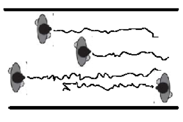
Figure 1: Zig-Zag phenomenon in movement of each pedestrian

Dynamic model of integer order that brought out by Dirk Helbing in [2, 3] has been extended to the following dynamic model of fractional order for each pedestrian

$$\left\{\begin{aligned} \frac{d^{\alpha}x_{i}}{dt^{\alpha}}&=v_{i},\\ m_{i}\frac{d^{\alpha}v_{i}}{dt^{\alpha}}&=f_{i}^{S}+\sum_{j=1}^{n}f_{ij}^{N}+\sum f_{k}^{W}.\end{aligned}\right.$$ (3)

where $x_{i}$ and $v_{i}$ are position and velocity of each pedestrian (2) respectively, $f_{i}^{S}$ is the self-driven force towards some desired velocity, $f_{ij}^{N}$ is the interaction between agent $i$ and its neighbor $j$ and $f_{k}^{W}$ represents the interactions with environment such as walls or corridors.

3.2 Fractional Macroscopic Model

As fractal time and space have been neglected in previous modeling of crowds, only macroscopic models of integer order have been been obtained in previous research. Some statistical phenomenons observed in recent years have forced people to reconsider the effectiveness of obtained dynamic model of integer order.

• Distribution of inter-event time that dominating or affecting movement of single pedestrian can be better approximated by power law rather than exponential distribution [1]. Thus dynamic models of integer order where exponential distribution has been assumed are no longer effective any more when confronted with the distribution of power law. As the hidden dynamics behind distribution of power law is fractional order, it is much preferred to model crowds of pedestrians using calculus of fractional order;

• Different to particles of gases or fluids, pedestrians do not fill the 2D or 3D space and distribution of the pedestrians is not uniform in the entire space. Thus space of integer order is not enough to describe the distribution of pedestrians and fractal space of fractional order should be included in modeling of crowds of pedestrians.

Based on [9] where modeling traffic system has been considered using calculus of integer order, we try to model crowds of pedestrians using calculus of fractional order in the followings.

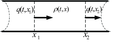
Figure 2: Conservation of Mass

Denote $\rho(x,t)$ as the density of crowds as shown in Figure 2, then mass of pedestrians between $x=x_{1}$ to $x=x_{2}$ at time $t$ can be computed as

$$\mbox{mass in}[x_{1},x_{2}]\mbox{ at time}\,t\,:=\int_{x_{1}}^{x_{2}}\rho(x,t)dx^{\beta}.$$ (4)

For $t\in[t_{1},t_{2}],$ the total mass that enters this domain from the left boundary at $x=x_{1}$ is given by

$$\mbox{inflow at}\,x_{1}\mbox{from}\,t_{1}\,\mbox{to}\,t_{2}\,:=\!\!\int_{t_{1}}^{t_{2}}\rho(x_{1},t)v(t,x_{1})dt^{\alpha}$$ (5)

Similarly, the total mass that leaves this domain from the right boundary at $x=x_{2}$ for $t\in[t_{1},t_{2}]$ is given by

$$\mbox{outflow at}\,x_{2}\,\mbox{from}\,t_{1}\,\mbox{to}\,t_{2}\,:=\!\!\!\int_{t_{1}}^{t_{2}}\!\!\!\rho(x_{2},t)v(t,x_{2})dt^{\alpha}$$ (6)

As the number of people in the area between $x_{1}$ and $x_{2}$ can change in time due to people crossing the boundary of $x_{1}$ and $x_{2}$. Assuming no pedestrians are created or destroyed, then the change of number of pedestrians is only due to changes at these two boundaries. Thus changes of mass of pedestrians in space $[x_{1},x_{2}]$ on time interval $[t_{1},t_{2}]$ is equal to the mass that entering at $x_{1}$ minus that exiting from $x_{2}$. This conservation can be describe using

$$\int_{x_{1}}^{x_{2}}\!\!\!\!\rho(t_{2},x)dx^{\beta} \!\!-\!\!\int_{x_{1}}^{x_{2}}\!\!\!\!\rho(t_{1},x)dx^{\beta}=\int_{t_{1}}^{t_{2}}\!\!\!\!\rho(x_{1},t)v(t,x_{1})dt^{\alpha}\!\!-\!\!\int_{t_{1}}^{t_{2}}\!\!\!\!\rho(x_{2},t)v(t,x_{2})dt^{\alpha}$$

The above equation can also be written as the following double integral form

$$\int_{x_{1}}^{x_{2}}\int_{t_{1}}^{t_{2}}\frac{\partial}{\partial t^{\alpha}}\rho(t,x)+\frac{\partial}{\partial x^{\beta}}[\rho(t,x)v(t,x)]dt^{\alpha}dx^{\beta}=0$$ (7)

Since equation (7) should be satisfied for any $t$ and any $x$, the following fractional order model for crowds of pedestrians in one dimensional space

$$\frac{\partial}{\partial t^{\text{$\alpha$}}}\rho(t,x)+\frac{\partial}{\partial x^{\beta}}[\rho(t,x)v(t,x)]=0$$ (8)

can be derived where fractal time and fractal space have been included in (8).

Remark 4.

Part of the results of fractional model in macro scale has been firstly brought out in [27] and are listed here to guarantee the completeness.

Remark 5.

Similar results are also obtained in [32] where fractional model for traffic flow has been derived using fractional conservation law. Different to the work of [32] where dimension of time is $\alpha$, dimension of surface is $2\alpha$ and dimension of volume is $3\alpha$, there are no such restrictions in our fractional model (8).

3.3 Fractional Micro-Macro Model

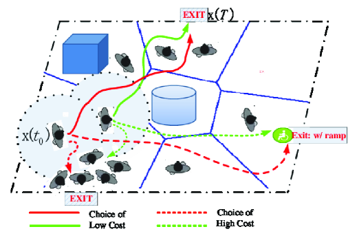
Figure 3: Movement of pedestrians based on fractional Mean Field Games

3.3.1 Fractional Hamilton-Jacobi-Bellman Equation

For each pedestrian $i$, we assume the following cost function to be minimized in his movement between initial starting point $x(t_{0})=x_{0}$ and desired location $x(T)$ as shown in Figure 3

$$J(t_{0},x_{0})=\underset{v(\cdot)}{inf}\int_{t_{0}}^{T}f(t,x(t),v(t))dt^{\alpha}+h(T,x(T)),$$ (9)

where convex function $h(T,x(T))$ is the terminal cost, convex even function $f(t,x(t),v(t))$ describes some different kinds of running cost between the initial point and destination.

Remark 6.

A typical quadratic cost function that independent on position of pedestrians can be selected as $\frac{1}{2}|v|^{2}$ to penalize pedestrians that moving too fast; Much more generalized running cost functions that depending on time, position and velocity have been are adopted in the following derivation of fractional Hamilton-Jacobi-Bellman Equation.

Similar to the derivation of Hamilton-Jacobi-Bellman equation of integer order in optimal control, the fractional Hamilton-Jacobi-Bellman Equation will be discussed firstly and then optimal velocity will prescribed for each pedestrian at each time step. Suppose after an infinitesimal time interval $dt^{\alpha}$, the pedestrian will arrived at one new place $x_{0}+vdt^{\alpha}$ and thus incurring a travel cost of $f(v)dt^{\alpha}$ where new cost function for the remaining journey described by $J(t_{0}+dt^{\alpha},x_{0}+vdt^{\alpha})$. The above analysis leads to the following relationship between $J(t_{0},x_{0})$ and $J(t_{0}+dt^{\alpha},x_{0}+vdt^{\alpha})$

$$J(t_{0},x_{0})=J(t_{0}+dt^{\alpha},x_{0}+vdt^{\alpha})+f(v)dt^{\alpha}.$$ (10)

Based on Taylor expansion, equation (10) can be rewritten as

$$J(t_{0},x_{0})=J(t_{0},x_{0}) +dt^{\alpha}[\frac{\partial^{\alpha}}{\partial t^{\alpha}}J(t_{0},x_{0})+v\cdot\frac{\partial^{\beta}}{\partial x^{\beta}}J(t_{0},x_{0})+f(v)],$$ (11)

and the optimal problem (9) is now transformed into finding proper $v$ to minimize

$$v\cdot\frac{\partial^{\beta}}{\partial x^{\beta}}J(t_{0},x_{0})+f(v).$$

Considering the fact that $f(\cdot)$ is an even function, the above minimizing problem is equivalent to the maximizing problem of

$$v\cdot\frac{\partial^{\beta}}{\partial x^{\beta}}J(t_{0},x_{0})-f(v).$$ (12)

Based on the Legendre transformation $H:R^{d}\rightarrow R$ of $f:R^{d}\rightarrow R$ by

$$H(p)\text{:=}\underset{v(\cdot)}{sup}\,v\cdot p-f(v)$$ (13)

whose maximum value are functions of $p$. For the maximum problem of (12) , we can see that the maximum value is obtained as $H(\frac{\partial^{\beta}}{\partial x^{\beta}}J(t_{0},x_{0})$) for some $v$. Then substituting the minimum value $-H(\frac{\partial^{\beta}}{\partial x^{\beta}}J(t_{0},x_{0}))$ into equation (11), the following equation

$$J(t_{0},x_{0})=J(t_{0},x_{0})+dt^{\alpha}[\frac{\partial^{\alpha}}{\partial t^{\alpha}}J(t_{0},x_{0})-H(\frac{\partial^{\beta}}{\partial x^{\beta}}J(t_{0},x_{0}))]$$

will be satisfied for any $t_{0}$ and any $x_{0}.$ Then the fractional Hamilton-Jacobi-Bellman Equation is derived as

$$-\frac{\partial^{\alpha}}{\partial t^{\alpha}}J(t_{0},x_{0})+H(\frac{\partial^{\beta}}{\partial x^{\beta}}J(t_{0},x_{0}))=0.$$ (14)

From the above discussions, we know that there are some $v$ that minimize the following expression

$$v\cdot\frac{\partial^{\beta}}{\partial x^{\beta}}J(t_{0},x_{0})+f(v),$$

and $\widetilde{v}=-v$ maximize the following expression

$$v\cdot\frac{\partial^{\beta}}{\partial x^{\beta}}J(t_{0},x_{0})-f(v).$$

As seen from (13), $\widetilde{v}$ as a function of $p$ should satisfy that

$$\frac{\partial}{\partial\widetilde{v}}(\widetilde{v}\cdot p-f(\widetilde{v}))=0.$$

On the other hand, the derivative of $H(p)$ can be obtained as follows

$$\frac{d}{dp}H(p)=\frac{\partial H}{\partial\widetilde{v}}\frac{\partial\widetilde{v}}{\partial p}+\frac{\partial H}{\partial p}=\widetilde{v},$$

using chain rule and then the velocity for each pedestrian to move in the next step is derived as

$$v=-H^{\prime}(\frac{\partial^{\beta}}{\partial x^{\beta}}J(t_{0},x_{0})).$$

3.3.2 Fractional Macro model based on Fractional Mean Field Games

Based on inspiration of [25] on traffic system, we assume the following utility function for the $i^{th}$ pedestrian

$$f_{i}^{N}(x_{i},v_{i})=v_{i}(1-F(\frac{1}{N}\sum\omega(x_{j}-x_{i}))),$$

where the first term $v_{i}$ means that the $i^{th}$ pedestrian try to arrive his destination as fast as possible; the second term means that the $i^{th}$ pedestrian adapts his velocity according to pedestrians around him. Bounded non-negative anticipating function $\omega(\cdot)$ has been introduced to weight different impacts of pedestrians in the neighborhood of the $i^{th}$ pedestrian according to their distances. Thus for the $i^{th}$ pedestrian, cooperative and competitive interacting with other pedestrians are manifested through choosing velocity on the next step.

First, we show that the following expression is satisfied

$$\lim_{N\rightarrow\infty}\frac{1}{N}\sum\omega(x_{j}-x_{i})\rightarrow\int_{0}^{\infty}\rho_{t}(y)\omega(y-x)dy^{\beta},$$

where $N$ is the number of interacting pedestrians, $\rho_{t}(y)$ is the number of pedestrians in interval $[x,x+dx^{\beta}]$ and $\omega(\cdot)$ is the anticipating function mentioned above.

Denote $\varGamma_{t}^{N}(x)=\frac{1}{N}\sum 1_{\{x_{j}<x\}}$ as the empirical distribution function for the crowds composed of $N$ pedestrians. Then based on the Lebesgue-Stieltjes integral it can be concluded that

$$\frac{1}{N}\sum\omega(x_{j}-x_{i})=\int_{0}^{\infty}\omega(y-x)d\varGamma_{t}^{N}(y).$$

If there is one non-decreasing right-continuous function $\varGamma_{t}(x)$ such that the following expression is satisfied

$$\int_{0}^{\infty}\omega(y-x)d\varGamma_{t}^{N}(y)\rightarrow\int_{0}^{\infty}\omega(y-x)d\varGamma_{t}(y)(N\rightarrow\infty).$$

Then

$$\frac{1}{N}\sum\omega(x_{j}-x_{i})\rightarrow\int_{0}^{\infty}\rho_{t}(y)\omega(y-x)dy^{\beta}(N\rightarrow\infty)$$

will be satisfied. As $\rho_{t}(y)$ is the number of pedestrians in interval $[x,x+dx^{\beta}]$, existence of non-decreasing right-continuous function $\varGamma_{t}(x)$ can be guaranteed from $d\varGamma_{t}(x)=\rho_{t}(x)dx^{\beta}.$ Thus we can impose the following mean filed payoff function

$$J(t_{0},x_{0},\rho_{t}(x))= \underset{v(\cdot)}{sup}\int_{t_{0}}^{T}\!\!v(1\!-\!F(\int_{0}^{\infty}\!\!\rho_{t}(y)\omega(y-x)dy^{\beta}))dt^{\alpha}+h(T,x(T))$$

for pedestrians that competitively and cooperatively interacting with other pedestrians.

Based on similar derivations shown in Section 3.3.1, the following fractional Hamilton-Jacobi-Bellman Equation

$$-\frac{\partial^{\alpha}}{\partial t^{\alpha}}J(t_{0},x_{0})+H(\frac{\partial^{\beta}}{\partial x^{\beta}}J(t_{0},x_{0},\rho_{t}(x)))=0$$

can also be obtained for modeling cooperative and competitive crowds using mean field game theory when the number of pedestrians goes to infinity.

Remark 7.

Difference to previous work are listed as followings:

• Only function of Dirac type and exponential type for $\omega(x_{j}-x_{i})$ have been considered in [25]. Anticipating function of inverse power form

  $$f_{i}^{N}(x_{i},v_{i})=v_{i}[1-F(\frac{1}{N}\sum(\left|x_{j}-x_{i}\right|+1){}^{-2})]$$

  can be included in this paper considering the long range effects in interacting of multiple pedestrians, where $\frac{1}{N}$ has been introduced to bound effects of other pedestrians on the $i^{th}$ pedestrian.

  • Mean field games theory is also utilized in [20] for modeling crowds of pedestrians. But obtained results of [20] are only restricted to the framework of calculus of integer order and many statistical characters are not considered such as power law in distribution of crowds, power law in distribution of inter-event time and long range interactions among pedestrians.

3.3.3 Fractional micro-macro model

As shown in Figure 4, the fractional micro-macro model for crowds of pedestrians using fractional mean field games can be described as the following backward-forward PDE systems

$$\left\{\begin{aligned} -\frac{\partial^{\alpha}}{\partial t^{\alpha}}J(t_{0},x_{0},\rho_{t}(x))\!+\!H(\frac{\partial^{\beta}}{\partial x^{\beta}}J(t_{0},x_{0},\rho_{t}(x)))&\!=0,\\ \frac{\partial}{\partial t^{\text{$\alpha$}}}\rho(t,x)\!+\!\frac{\partial}{\partial x^{\beta}}[\rho(t,x)v(t,x)]&\!=0,\end{aligned}\right.$$ (15)

and

$$\left\{\begin{aligned} \frac{d^{\alpha}x_{i}}{dt^{\alpha}}&=v_{i},\\ m_{i}\frac{d^{\alpha}v_{i}}{dt^{\alpha}}&=f_{i}^{S}+\sum_{j=1}^{n}f_{ij}^{N}+\sum f_{k}^{W}.\end{aligned}\right.$$ (16)

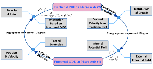
Figure 4: Fractional Micro-Macro model of Crowds of Pedestrians

The fractional microscopic model and fractional macroscopic model are connected through aggregation and disaggregation on Voronoi Diagram. From Figure 4, the followings can be observed.

1. Movements of each microscopic model are determined by not only internal potential fields such as the self-driven force towards some desired velocity described using $f_{i}^{S}$ in (16) but also external interactions from neighbors and environments which described using $f_{ij}^{N}$ and $f_{k}^{W}$. Some other elements such as deviations from optimal movement of the whole crowds are also playing an important role in the movement of each individual pedestrian. All these information should generated from the dynamic model in macro scale;

2. Density and velocity that needed in macroscopic model are derived from aggregation of individual’s position and velocity. When the number of pedestrians goes to infinity, the crowds of pedestrians are treated as some intelligent flows that described with the help of fractional MFG as shown in (15). For the backward part, $v$ can be solved from the first line of equation (15) under initial condition on $J(T,X_{T})$ and initial distribution of $\rho_{0}(x)$ derived from aggregation of microscopic model (16); Then substitute the obtained $v$

   $$v=-H^{\prime}(\frac{\partial^{\beta}}{\partial x^{\beta}}J(t_{0},x_{0},\rho_{t}(x)))$$

   into the forward part and $\rho(t,x)$ will be obtained from the second line of equation (15) under initial condition $\rho_{0}(x)$.

Due to the complexity of crowds of pedestrians, fractional microscopic model and fractional macroscopic model that interacted with each other have been constructed in this paper. Fractional mean field games have also been utilized in describing the macroscopic model when the number of pedestrians goes to infinity.

Remark 8.

To the author’s knowledge, the paper is one of the first works applying fractional mean field games to fractional macroscopic and microscopic model for competitive and cooperative crowds of pedestrians. Although some theoretical work has been obtained, a lot of work are waiting for further efforts such as existence and uniqueness of solution, rate of convergence and stability of desired equilibrium.

4 Simulation Results

Considering unexpected or dangerous events in real-life experiment, only some initial simulation results are conducted to show the differences between model of fractional order and model of integer order in macro scale and micro scale. Due to the difficulties caused when the number of pedestrians goes to infinity, simulation results in macro scale and micro scale are separated in the following subsections. All we want to show is that calculus of fractional order has offered us much more freedom in describing complex phenomenon or dynamics such as crowds of pedestrians. It is much preferred to choose different model according to different scenarios and there are a lot of interesting problems needing to be considered in future.

4.1 Fractional Macroscopic Model

4.1.1 Simulation in closed and square area without exit

Simulation results on fractional macroscopic model (8) are firstly conducted where $\beta=1$ are imposed for simplicity. Lax-Friedrichs Scheme has been used to approximate the spatial derivatives in solving the nonlinear partial differential equations due to its efficiency in computation. Based on Lax-Friedrichs Scheme, the following PDE on 2D plane

$$\frac{\partial}{\partial t^{\text{$\alpha$}}}\rho(t,x,y) +\frac{\partial}{\partial x}[\rho(t,x,y)v(t,x,y)]+\frac{\partial}{\partial y}[\rho(t,x,y)v(t,x,y)]=0$$

has been transformed into

$$\begin{array}[]{c}\frac{\partial}{\partial t^{\text{$\alpha$}}}\rho(t,x,y)+\frac{1}{2Dx}[\rho(t,x+1,y)v(t,x+1,y)\\ -\rho(t,x-1,y)v(t,x-1,y)]+\frac{1}{2Dy}[\rho(t,x,y+1)v(t,x,y+1)-\rho(t,x,y-1)v(t,x,y-1)]=0\end{array}$$

in the simulations.

Under the following initial Gaussian distribution

$$\rho(x,y,0)=C\exp(-(x-a)^{2}-(y-b)^{2}),$$

where $C=1$ is the density value and $(a,b)$ determines the center of initial density distribution. Average speed of free flow has been chosen to be $v_{x}=v_{y}=1.36ms^{-1}$as done in many previous studies for pedestrians. Pedestrians have also been assumed to move freely within a square area with no obstacles and no exits in the first simulations.

Simulation results for $\alpha=0.6$ and $\alpha=1$ are shown in Figure 5 to 6 and Figure 7 to 8, respectively. From Figure 5 and Figure 7, it can be concluded that pedestrians described using fractional model are much scattered in the closed square area than that described using model of integer order. Same conclusions can also be obtained from comparisons between Figure 6 and Figure 8. Other fractional orders can also be tested using the methods proposed in this paper but data from reality are much preferred to find the proper orders for modeling the crowds of pedestrians in macro scale.

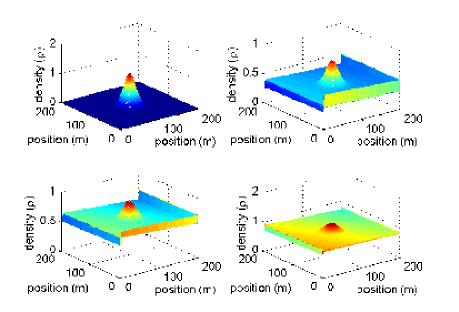
Figure 5: Density response for crowds of pedestrians with $\alpha=0.6$ using Lax-Friedrichs Scheme

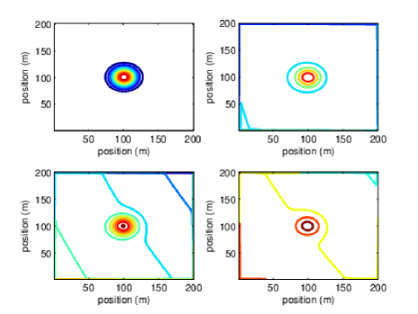
Figure 6: Contour of the density response for crowds of pedestrians with $\alpha=0.6$ using Lax-Friedrichs Scheme

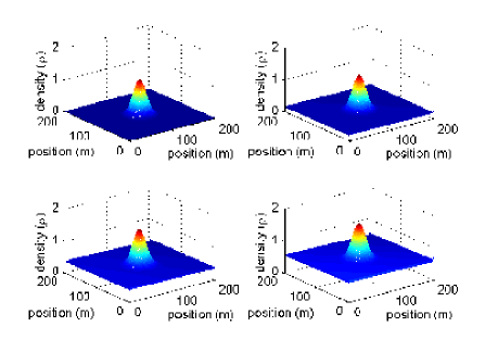
Figure 7: Density response for crowds of pedestrians of integer order using Lax-Friedrichs Scheme

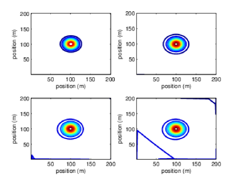
Figure 8: Contour of the density response for crowds of pedestrians of integer order using Lax-Friedrichs Scheme

4.1.2 Simulation in closed and square area with one exit

Based on results obtained in Section 4.1.1, the following dynamic model has been simulated for pedestrians in closed and square area with one exit

$$\left\{\begin{aligned} \frac{\partial}{\partial t^{\text{$\alpha$}}}\rho(t,x,y)+\frac{\partial}{\partial x}&[\rho(t,x,y)v(t,x,y)]\\ +\frac{\partial}{\partial y}&[\rho(t,x,y)v(t,x,y)]=0,\\ v_{t}+vv_{x}\,\,\,\,&=\frac{V-v}{\tau}-\frac{C_{0}^{2}}{\rho}\rho_{x},\\ u_{t}+uu_{y}\,\,\,\,&=\frac{U-u}{\tau}-\frac{C_{0}^{2}}{\rho}\rho_{y},\end{aligned}\right.$$

where $C_{0}=0.8$ is the anticipation term that describes the response of pedestrians to density of people and $V$ and $U$ are some desired velocity that obtained for the crowds. In order to lead the crowd moving toward the exit, the desired velocity $V$ and $U$ are selected as done in [33]

$$\left\{\begin{array}[]{cc}V=&V(\rho)\frac{x_{e}-x_{i}}{\sqrt{(x_{e}-x_{i})^{2}+(y_{e}-y_{i})^{2}}}\\ U=&U(\rho)\frac{y_{e}-y_{i}}{\sqrt{(x_{e}-x_{i})^{2}+(y_{e}-y_{i})^{2}}}\end{array}\right.$$

where $V(\rho)$ and $U(\rho)$ are the flux-density relationship for Greenshield’s model.

Simulation results are shown in Figure 9 and Figure 10 where dynamic model with fractional order $0.85$ and $1$ are used. Simulation results show that the density of pedestrians around the exit is much lower in model of fractional order than that obtained using model of integer order. In simulations, the authors found that the stable density of pedestrians is depending on the fractional order selected in the simulation and how to choose the best order to model the dynamics of crowds is an interesting problem that is worthy of further consideration in future research.

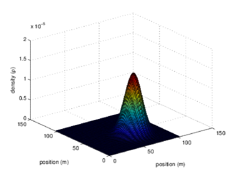
Figure 9: Density response for crowds of pedestrians with $\alpha=0.85$ using Lax-Friedrichs Scheme

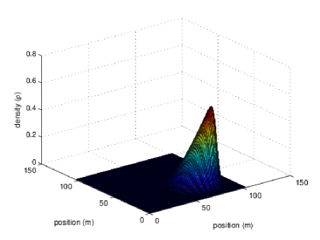
Figure 10: Contour of the density response for crowds of pedestrians with $\alpha=1$ using Lax-Friedrichs Scheme

4.2 Fractional Microscopic Model

In this section, six pedestrians with fractional order $\alpha\in(0,1)$, $\alpha=1$ and $\alpha\in(1,2)$ are employed respectively to show their effects on pedestrian’s evacuation process. Simulations of crowds of pedestrians with fractional order $\alpha=0.6$, $\alpha=1$ and $\alpha=1.3$ are shown in Figure 11, Figure 12 and Figure 13 respectively. Results show that all agents firstly reach consensus through interacting with their neighbors without games. But parts of them changed their desired value and fragmentation phenomenon are observed through these simulations after some penalty terms are injected into the simulations. Obtained simulation results have shown that pedestrians with different orders have different performance. Thus Fractional Calculus has provided us much more freedom in analysis and control of this kind of complex system. How to quantitatively characterize the relationship between order of fractional model, fractional controller and fractional games are interesting topics to be considered for the authors.

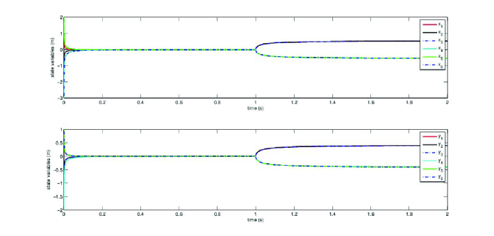
Figure 11: Responses of six pedestrians with $\alpha=0.6$

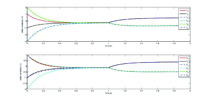
Figure 12: Responses of six pedestrians with $\alpha=1$

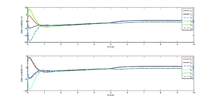
Figure 13: Responses of six pedestrians with $\alpha=1.3$

5 Conclusions

Modeling of crowds of pedestrians have been considered in this paper from the view of Fractional Calculus. Not only fractional microscopic models but also fractional macroscopic models have been proposed in this paper. Fractional mean field games theory have been introduced in the modeling of crowds of pedestrians and coupled PDEs composed of fractional backward part and fractional forward part have been investigated. Although some theoretical results and some initial simulations are presented in this paper, there are much more work unexplored along this topic, such as solution of fractal MFG systems, stability of the fractal MFG system and performance of this fractal system, controller design based on mean field, performance evaluation of dynamic crowds and security problems related to control of crowds.

References

- [1] Bruce J. West, Malgorzata Turalska, and Paolo Grigolini. Networks of Echoes Imitation, Innovation and Invisible Leaders, volume Computatio. Springer International Publishing Switzerland, 2014.
- [2] Helbing Dirk and Molnar Peter. Social force model for pedestrian dynamics. Physical Review E, 51:4282–4286, 1995.
- [3] Dirk Helbing, Illes Farkas, and Tamas Vicsek. Simulating dynamical features of escape panic. Nature, 407(28):487–490, 2000.
- [4] Nicola Bellomo, C. Bianca, and V. Coscia. On the modeling of crowd dynamics: an overview and research perspectives. SeMA Journal, 54(1):25–46, 2013.
- [5] Couzin Iain D., Krause Jens, Franks Nigel R., and Levin Simon A. Effective leadership and decision-making in animal groups on the move. Nature, 433:513–516, 2005.
- [6] Iain D. Couzin. Collective cognition in animal groups. Trends in Cognitive Sciences, 13(1):36–43, 2008.
- [7] Weiguo Song, Xuan Xu, Bing-Hong Wang, and Shunjiang Ni. Simulation of evacuation processes using a multi-grid model for pedestrian dynamics. Physica A, 363:492–500, 2006.
- [8] Nirajan Shiwakoti, Majid Sarvi, Geoff Rose, and Martin Burd. Animal dynamics based approach for modeling pedestrian crowd egress under panic conditions. Transportation Research Part B, 45(9):1433–1449, 2011.
- [9] Pushkin Kachroo. Pedestrian Dynamics: Mathematical Theory and Evacuation Control. CRC Press, Taylor & Francis Group, 2009.
- [10] Dirk Helbing. A fluid dynamic model for the movement of pedestrians. Complex Systems, 6:391–415, 1992.
- [11] Roger L. Hughes. A continuum theory for the flow of pedestrians. Transportation Research Part B: Methodological, 36(6):507–535, 2002.
- [12] Roger L. Hughes. The flow of human crowds. Annual Review of Fluid Mechanics, 35:169–182, 2003.
- [13] Jiang Yan-qun, Zhang Peng, Wong S.C., and Liu Ru-xun. A higher-order macroscopic model for pedestrian flows. Physica A: Statistical Mechanics and its Applications, 389(21):4623–4635, 2010.
- [14] Sadeq J. Al-nasur. New Models for Crowd Dynamics and Control. PhD thesis, Virginia Polytechnic Institute and State University, 2006.
- [15] Corrado Lattanzio, Amelio Maurizi, and Benedetto Piccoli. Moving bottlenecks in car traffic flow a pde-ode coupled model. Society for Industrial and Applied Mathematics, 43(1):50–67, 2011.
- [16] Ryosuke Ishiwata and Yuki Sugiyama. Relationships between power-law long-range interactions and fractional mechanics. Physica A, 391(23):5827–5838, 2012.
- [17] Yves Achdou, Fabio Camilli, and Italo Capuzzo-Dolcetta. Mean field games numerical methods for the planning problem. SIAM Journal on Control and Optimization, 50(1):77–109, 2012.
- [18] Peter E. Caines. Mean field stochastic control peter e. caines. Technical report, IEEE Control Systems Society Bode Lecture, 48th Conference on Decision and Control, 2009.
- [19] Guéant Olivier. A reference case for mean field games models. J. Math. Pures Appl., 92(3):276–294, 2009.
- [20] Christian Dogbe. Modeling crowd dynamics by the mean-field limit approach. Mathematical and Computer Modelling, 52(9-10):1506–1520, 2010.
- [21] Nourian Mojtaba, Malhame Roland P., Huang Minyi, and Caines Peter E. Mean field (nce) formulation of estimation based leader-follower collective dynamics. International Journal of Robotics & Automation, 26(1):120–129, 2011.
- [22] Mojtaba Nourian, Peter E. Caines, Roland P. Malhame, and Minyi Huang. Mean field lqg control in leader-follower stochastic multi-agent systems likelihood ratio based adaptation. IEEE Transactions on Automatic Control57, 57(11):2801–2816, 2012.
- [23] Mojtaba Nourian, Peter E. Caines, Roland P. Malhame, and Minyi Huang. Nash, social and centralized solutions to consensus problems via mean field control theory. IEEE Transactions on Automatic Control, 58(3):639–653, 2013.
- [24] Aime Lachapelle and Marie-Therese Wolfram. On a mean field game approach modeling congestion and aversion in pedestrian crowds. Transportation Research Part B: Methodological, 45(10):1572–1589, 2011.
- [25] Geoffroy Chevalier, Jerome Le Ny, and Roland Malhame. A micro-macro traffic model based on mean-field games. In 2015 American Control Conference, Palmer House Hilton, July 1-3, 2015. Chicago, IL, USA, 2015.
- [26] Paul Bogdan and Radu Marculescu. A fractional calculus approach to modeling fractal dynamic games. In IEEE Conference on Decision and Control and European Control Conference, pages 255–260, 2011.
- [27] Ke-Cai Cao, Caibin Zeng, Dan Stuart, and YangQuan Chen. Fractional order dynamic modeling of crowd pedestrians. In The Fifth Symposium on Fractional Differentiation and Its Applications, 2012.
- [28] Kecai Cao, Yangquan Chen, Dan Stuart, and Dong Yue. Cyber-physical modeling and control of crowd of pedestrians: a review and new framework. Automatica Sinica, IEEE/CAA Journal of, 2(3):334–344., 2015. http://arxiv.org/abs/1506.05340.
- [29] Ke-Cai Cao, YangQuan Chen, and Dan Stuart. A new fractional order dynamic model for human crowd stampede system. In The 2015 Symposium on Fractional Derivatives and Their Applications, Boston, USA, pages DETC2015–47007, 2015.
- [30] Abhay Parvate and A D Gangal. Fractal differential equations and fractal-time dynamical systems. PRAMANA Indian Academy of Sciences, 64(3):389–409, 2005.
- [31] Shantanu Das. Functional Fractional Calculus. Springer-Verlag Berlin Heidelberg, 2011.
- [32] Long-Fei Wang, Xiao-Jun Yang, Dumitru Baleanu, Carlo Cattani, and Yang Zhao. Fractal dynamical model of vehicular traffic flow within the local fractional conservation laws. Abstract and Applied Analysis, pages 1–5, 2014.
- [33] Pushkin Kachroo, Sadeq J. Al-nasur, Sabiha Amin Wadoo, and Apoorva Shende. Pedestrian Dynamics Feedback Control of Crowd Evacuation. Springer-Verlag Berlin Heidelberg, 2008.