A simple proof of the detectability lemma and spectral gap amplification

Abstract

The detectability lemma is a useful tool for probing the structure of gapped ground states of frustration-free Hamiltonians of lattice spin models. The lemma provides an estimate on the error incurred by approximating the ground space projector with a product of local projectors. We provide a new, simpler proof for the detectability lemma which applies to an arbitrary ordering of the local projectors, and show that it is tight up to a constant factor. As an application, we show how the lemma can be combined with a strong converse by Gao to obtain local spectral gap amplification: We show that by coarse graining a local frustration-free Hamiltonian with a spectral gap $\gamma>0$ to a length scale $\operatorname{O}\bigl{(}\gamma^{-1/2}\bigr{)}$, one gets a Hamiltonian with an $\operatorname{\Omega}\bigl{(}1\bigr{)}$ spectral gap.

I Introduction

In recent years our understanding of quantum many-body systems, and in particular the properties of their ground states, has shown considerable progress. Much of this understanding can be attributed to the development of new technical tools for analyzing general many-body quantum systems. A particularly powerful set of techniques, pioneered by Hastings[1], uses Lieb-Robinson bounds[2, 3] together with appropriate filtering functions to construct local approximations to the action of the ground state projector. These techniques were successfully leveraged to rigorously establish many interesting properties of ground states such as exponential decay of correlations in gapped models[1, 4, 3], an area law for one-dimensional (1D) gapped systems[5], efficient classical simulation of adiabatic evolution of 1D gapped systems[6, 7], stability of topological order[8, 9], classification of quantum phases[10], and many more (see, e.g., LABEL:ref:Hastings2010-locality and references therein).

More recently, originating in an attempt to tackle some aspects of the quantum PCP conjecture[12], a new tool has been introduced for the analysis of many-body local Hamiltonians, known as the detectability lemma (DL)[13]. The DL has proven particularly useful for studying the ground states of gapped, frustration-free spin systems on a lattice[14]. Examples of such systems include the Affleck-Kennedy-Lieb-Tasaki (AKLT) model [15], the spin $1/2$ ferromagnetic XXZ chain[16] and Kitaev’s toric code [17, 18].

Given a local Hamiltonian $H$ that is frustration free, the detectability lemma operator $\mathop{\rm DL}\nolimits(H)$ is defined as a product of the local ground space projectors associated to each term in the Hamiltonian, organized in layers (see Fig. 1 and Sec. III for a precise statement). The DL operator leaves the ground space of $H$ invariant while shrinking all excited states by a factor of at least $1-\Delta$ for some $0<\Delta<1$. The detectability lemma establishes a lower bound on $\Delta$, thereby placing an upper bound on the shrinking of any state orthogonal to the ground space. Essentially, the lemma shows that $\Delta$ is at least a constant times the spectral gap of $H$.

Since the DL operator preserves the ground space and shrinks any state orthogonal to it, it can be viewed as an approximation to the ground state projector, with an error of $1-\Delta$. This allows one to approximate the highly complex and possibly non-local ground space projector of the full system by the simpler operator $\mathop{\rm DL}\nolimits(H)$ (or a power of it). It provides a considerably simpler alternative to more general constructions based on Lieb-Robinson bound and the use of filtering functions (admittedly those constructions also apply to frustrated systems). Many results that were proved for general systems using these techniques, such as the 1D area law and the exponential decay of correlations, can be proved in simpler way for the case of frustration-free systems using the DL [14]. In addition, the DL has found further applications such as the analysis of T-designs[19] and Gibbs samplers[20], and an improvement to the original 1D area law for frustration-free systems[21].

The original proof of the DL from LABEL:ref:AALV2009-gap-amp used the so-called XY decomposition and was limited to local Hamiltonians in which the local terms are taken from a constant set. Subsequently, a much simpler proof, which does not rely on the XY decomposition and is free of the limitations of the first proof, was introduced in LABEL:ref:AharoAVZ2011-DL. In this paper we introduce yet another proof of the DL, which is simpler than the proof of LABEL:ref:AharoAVZ2011-DL, provides a tighter bound on $1-\Delta$, and is more general as it holds for an arbitrary ordering of the local projectors. This tighter form of the DL has already been used in [22] to derive a quadratically improved upper bound on the correlation length of gapped ground states of frustration-free systems.

Recent work of Gao[23] on a quantum union bound establishes a converse to the DL that provides a lower bound on the spectral gap of a frustration-free Hamiltonian $H$ as a function of the spectral gap of $\mathop{\rm DL}\nolimits(H)$. Equivalently, Gao’s result places an upper bound on the parameter $\Delta$, or a lower bound on the shrinking of excited states by $\mathop{\rm DL}\nolimits(H)$ (see Lemma 4 for a precise statement). Together with the detectability lemma, the two results establish a form of duality between $H$ and $\mathop{\rm DL}\nolimits(H)$, showing that their spectral gaps are always within a constant factor from each other. This converse to the DL has already been used for the purpose of proving lower bounds on the spectral gap of frustration-free Hamiltonians in forthcoming work on 1D area laws and efficient algorithms[25].

As an application, in the second part of this paper we show how a combination of the DL and its converse can be used to prove that the spectral gap of a local frustration-free Hamiltonian can be amplified from $\gamma>0$ to a constant by coarse-graining the Hamiltonian to a length scale $\operatorname{O}\bigl{(}\gamma^{-1/2}\bigr{)}$. A direct application of both lemmas provides the result for a length scale $\operatorname{O}\bigl{(}\gamma^{-1}\bigr{)}$; we quadratically improve the dependence on $\gamma$ by employing a Chebyshev polynomial in a way analogous to recent work of Gosset and Huang [22].

Organization.

In Sec. III we state and prove the DL. In Sec. IV we give our application to spectral gap amplification.

II The DL operator and frustration-free spin systems on a lattice

Throughout we use the “big O” notation, where $\operatorname{O}\bigl{(}f(x)\bigr{)}$ indicates any function $g$ such that there is a constant $C>0$, $|g(x)|\leq C\cdot f(x)$ for all $x$ in the domain of $f$. Similarly, $\operatorname{\Omega}\bigl{(}f(x)\bigr{)}$ denotes any function $g$ such that there exists a constant $c>0$ such that $g(x)\geq c\cdot f(x)$ for all $x$ in the domain of $f$.

We concentrate on frustration-free spin systems on regular lattices. Formally, we consider $n$ quantum spins with local dimension $d$ that are positioned on the vertices of a regular $D$-dimensional lattice with an underlying Hilbert space $\mathcal{H}=(\mathbb{C}^{d})^{\otimes n}$. On this lattice we consider a $k$-local Hamiltonian system $H=\sum_{i}h_{i}$ where each $h_{i}$ acts on at most $k$ neighboring spins of the lattice. It is easy to see that in this setting every local term does not commute with at most $g$ other local terms, where $g$ is a constant. Moreover, the set of local terms can always be partitioned into $L$ subsets $T_{1},T_{2},\ldots,T_{L}$, called layers, such that each layer consists of non-overlapping local terms, which are therefore pairwise commuting. Clearly, both $g$ and $L$ can be upper bounded as functions of $k$ and $D$ [trivial bounds are $g\leq k(2D)^{k-1}$ and $L\leq(2D)^{2k}$]; for clarity, here we treat them as independent parameters. A canonical example is a spin chain over $n$ spins with nearest-neighbor interactions $H=\sum_{i=1}^{n-1}h_{i}$, where $h_{i}$ acts on spins $\{i,i+1\}$. Each $h_{i}$ is non-commuting with at most $g=2$ neighbors, and the system can be partitioned into $L=2$ layers, the odd layer $T_{\text{odd}}=\{h_{1},h_{3},h_{5},\ldots\}$ and the complementary even layer $T_{\text{even}}$. This decomposition is illustrated in Fig. 1.

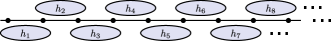
Figure 1: Decomposing the local terms of a 1D Hamiltonian $H=\sum_{i}h_{i}$ with 2-local, nearest-neighbor interactions into two layers — an even layer and an odd layer.

By adding constant multiples of the identity to each $h_{i}$ we may assume without loss of generality that their smallest eigenvalue is $0$. Moreover, assuming that the norms of the $h_{i}$ are uniformly bounded by a constant, we may scale the system and switch to dimensionless units in which $\|h_{i}\|\leq 1$ and therefore $0\leq h_{i}\leq\mathbbm{1}$. We label the energy levels of $H$ by $\epsilon_{0}<\epsilon_{1}<\epsilon_{2}\cdots$, where each level may correspond to more than one eigenstate of $H$. The ground space of $H$ is denoted by $V_{gs}$ and the projector onto it by $\Pi_{gs}$. We let $\gamma:=\epsilon_{1}-\epsilon_{0}>0$ denote the spectral gap of the system.

We say that the system is frustration free when every ground state $|\Omega\rangle\in V_{gs}$ minimizes the energy of each local term $h_{i}$ separately, i.e., $\langle\Omega|h_{i}|\Omega\rangle=0$. Notice that in such case it necessarily holds that $h_{i}|\Omega\rangle=0$ and hence every ground state is a common eigenstate of all $h_{i}$. This property strongly constrains the structure of frustration-free ground states and makes their analysis much simpler in comparison with the general frustrated case.

When studying frustration-free ground states it is often convenient to introduce an auxiliary Hamiltonian in which every $h_{i}$ is replaced by a projector $Q_{i}$ whose null space coincides with the null space of $h_{i}$. The auxiliary Hamiltonian $\hat{H}:=\sum_{i}Q_{i}$ and the original Hamiltonian $H=\sum_{i}h_{i}$ thus share the same ground space. Moreover, since $0\leq h_{i}\leq\mathbbm{1}$, $0\leq h_{i}\leq Q_{i}$, and $\hat{H}\geq H$. It follows that if $H$ is gapped, then so is $\hat{H}$, with $\gamma(\hat{H})\geq\gamma(H)$. Note that in case the original Hamiltonian $H=\sum_{i}a_{i}Q_{i}$ with $Q_{i}$ projectors and $0\leq a_{i}\leq 1$, the effect of this transformation is simply to set $\hat{H}=\sum_{i}Q_{i}$, a Hamiltonian with the same ground space and a gap at least as large as that of $H$. From here onwards in order to keep the notation light we shall denote $\hat{H}$ by $H$, or simply assume that $H$ itself is given as a sum of projectors, $H=\sum_{i}Q_{i}$.

A useful approach for understanding the locality properties of the ground space of $H$ consists in approximating its ground state projector $\Pi_{gs}$ by an operator that possesses a more local structure, and is therefore easier to work with. Such operators are referred to as Approximate Ground State Projectors (AGSPs), and various constructions have been used to establish properties of gapped ground states such as exponential decay of correlations[14, 22], area laws[21, 26], and local reversibility[27]. Frustration-free systems can be given a very natural construction of AGSP, called the detectability lemma operator $\mathop{\rm DL}\nolimits(H)$. To introduce this operator, define the layer projector $\Pi_{\ell}:=\prod_{i\in T_{\ell}}(\mathbbm{1}-Q_{i})$ for every layer $\ell$. As $\Pi_{\ell}$ is a product of commuting projectors, it is by itself a projector — the projector onto the ground space of the $\ell$-th layer. Then $\mathop{\rm DL}\nolimits(H)$ is defined as follows.

Definition 1 (The detectability lemma operator)

Given a decomposition of the terms of a local Hamiltonian $H=\sum_{i}Q_{i}$ in $L$ layers $T_{1},\ldots,T_{L}$ the detectability lemma operator of $H$ is defined as

$$\mathop{\rm DL}\nolimits(H):=\Pi_{L}\cdots\Pi_{1}=\prod_{\ell=1}^{L}\prod_{i\in T_{\ell}}(\mathbbm{1}-Q_{i}).$$ (1)

It is easy to see that $\mathop{\rm DL}\nolimits(H)$ is indeed an AGSP: by the frustration-free assumption each $\mathbbm{1}-Q_{i}$ preserves the ground space, hence $\mathop{\rm DL}\nolimits(H)V_{gs}=V_{gs}$. Moreover, $\|\mathop{\rm DL}\nolimits(H)\|\leq 1$, since its a product of projectors, and $\|\mathop{\rm DL}\nolimits(H)|\psi\rangle\|=1$ if and only if $|\psi\rangle\in V_{gs}$. Therefore, there exists some $0<\Delta<1$ such that for every state $|\psi^{\perp}\rangle$ that is perpendicular to the ground space, $\|\mathop{\rm DL}\nolimits(H)|\psi^{\perp}\rangle\|\leq 1-\Delta$. It follows that $\|\Pi_{gs}-\mathop{\rm DL}\nolimits(H)\|\leq 1-\Delta$. Therefore the DL operator is an AGSP, whose quality is determined by the parameter $\Delta$. Moreover, using again the fact that the system is frustration-free, one can amplify the quality of approximation by taking power of the DL operator: $\|\Pi_{gs}-\mathop{\rm DL}\nolimits^{q}(H)\|\leq(1-\Delta)^{q}$ for any $q\geq 1$.

As an operator, $\mathop{\rm DL}\nolimits^{q}(H)$ is an alternating product of layer projectors. Pictorially, it can be visualized as a stack of layers, much as a brick wall (see, e.g., Fig. 3). One can verify that the collection of projectors $\mathbbm{1}-Q_{i}$ appearing in $\mathop{\rm DL}\nolimits^{q}(H)$ that do not commute with a given local operator $B$ forms a “light cone” centered at $B$. This observation is crucial for understanding the effect of $B$ on the ground space, and is arguably the most important way in which locality of the DL operator can be leveraged.

We are left with the task of estimating the parameter $\Delta$. The detectability lemma, introduced in the next section, provides a lower bound on $\Delta$ (an upper bound on $1-\Delta$). The converse to the lemma, Lemma 4, provides an upper bound on $\Delta$. Crucially, even though both bounds depend on $\gamma$, and the bound from the DL also depends on $g$, both bounds are independent of the system size.

III A simple proof of the detectability lemma

The variant of the DL we are about to prove is more general that the one from LABEL:ref:AharoAVZ2011-DL in that the projectors $Q_{i}$ are not assumed to be local, nor placed on a fixed lattice; the order of their product in $\mathop{\rm DL}\nolimits(H)$ can be arbitrary. Luckily, the proof also turns out to be simpler than the original proof.

Lemma 2 (The detectability lemma (DL))

Let $\{Q_{1},\ldots,Q_{m}\}$ be a set of projectors and $H=\sum_{i=1}^{m}Q_{i}$. Assume that each $Q_{i}$ commutes with all but $g$ others. Given a state $|\psi\rangle$, define $|\phi\rangle:=\prod_{i=1}^{m}(\mathbbm{1}-Q_{i})|\psi\rangle$, where the product is taken in any order, and let $\epsilon_{\phi}:=\frac{1}{\|\phi\|^{2}}\langle\phi|H|\phi\rangle$ be its energy. Then

$$\big{\|}\prod_{i=1}^{m}(\mathbbm{1}-Q_{i})|\psi\rangle\big{\|}^{2}\leq\frac{1}{\epsilon_{\phi}/g^{2}+1}.$$ (2)

By choosing the order of the projectors to coincide with that in $\mathop{\rm DL}\nolimits(H)$ (for any decomposition into layers), and observing that for every state $|\psi^{\perp}\rangle$ orthogonal to the ground space it holds that $\langle\psi^{\perp}|H|\psi^{\perp}\rangle\geq\gamma$, we obtain the following immediate corollary.

Corollary 3

For any state $|\psi^{\perp}\rangle$ orthogonal to the ground space of $H$,

$$\|\mathop{\rm DL}\nolimits(H)|\psi^{\perp}\rangle\|^{2}\leq\frac{1}{\gamma/g^{2}+1}.$$ (3)

In light of the discussion in the Introduction, we see that the DL implies that $1-\Delta\leq\frac{1}{\sqrt{\gamma/g^{2}+1}}$, or, equivalently, $\Delta\geq 1-\frac{1}{\sqrt{\gamma/g^{2}+1}}\geq\gamma/(4g^{2})$, where the second inequality follows from the fact that $\gamma/g^{2}<1$. (To see this, note that a state of energy at most $g+1<g^{2}$ and orthogonal to the ground space can always be constructed by starting from any ground state and replacing the state of the spins associated with an arbitrary local term $h_{i}$ with a local state orthogonal to the ground space of $h_{i}$.)

We now turn to the proof of the DL; after the proof we give a simple example showing that the dependence on $g$ in the bound provided by the lemma is necessary.

• We start by considering

  $$\langle\phi|H|\phi\rangle=\sum_{i=1}^{m}\langle\phi|Q_{i}|\phi\rangle=\sum_{i=1}^{m}\|Q_{i}|\phi\rangle\|^{2}.$$

  To bound $\|Q_{i}|\phi\rangle\|$ we write it as $\|Q_{i}(\mathbbm{1}-Q_{m})\cdots(\mathbbm{1}-Q_{1})|\psi\rangle\|$ and try to move $Q_{i}$ to the right until it hits $(\mathbbm{1}-Q_{i})$ and vanishes. Let $N_{i}$ denote the subset of indices of projectors that do not commute with $Q_{i}$. Whenever $j\in N_{i}$, we use the triangle inequality to write

  $$\|Q_{i}(\mathbbm{1}-Q_{j})\cdot(\mathbbm{1}-Q_{j-1})\cdots(\mathbbm{1}-Q_{1})|\psi\rangle\|$$

  $$\leq\|Q_{i}(\mathbbm{1}-Q_{j-1})\cdots(\mathbbm{1}-Q_{1})|\psi\rangle\|$$

  $$\ \ +\|Q_{i}Q_{j}(\mathbbm{1}-Q_{j-1})\cdots(\mathbbm{1}-Q_{1})|\psi\rangle\|.$$

  Therefore,

  $$\|Q_{i}|\phi\rangle\|\leq\sum_{j\in N_{i}}\|Q_{j}(\mathbbm{1}-Q_{j-1})\cdots(\mathbbm{1}-Q_{1})|\psi\rangle\|,$$

  where we also used $\|Q_{i}\|\leq 1$. Since $|N_{i}|\leq g$, we get

  $$\|Q_{i}|\phi\rangle\|^{2}\leq g\sum_{j\in N_{i}}\|Q_{j}(\mathbbm{1}-Q_{j-1})\cdots(\mathbbm{1}-Q_{1})|\psi\rangle\|^{2}.$$

  Summing over $i=1,\ldots,m$, each term $\|Q_{j}(\mathbbm{1}-Q_{j-1})\cdots(\mathbbm{1}-Q_{1})|\psi\rangle\|^{2}$ appears at most $g$ time because there are at most $g$ projectors $Q_{i}$ that do not commute with $Q_{j}$. Thus

  $$\langle\phi|H|\phi\rangle =\sum_{i}\langle\phi|Q_{i}|\phi\rangle=\sum_{i}\|Q_{i}|\phi\rangle\|^{2}$$

  $$\leq g^{2}\sum_{j=2}^{m}\|Q_{j}(\mathbbm{1}-Q_{j-1})\cdots(\mathbbm{1}-Q_{1})|\psi\rangle\|^{2}$$

  $$=g^{2}\big{[}\|(\mathbbm{1}-Q_{1})|\psi\rangle\|^{2}$$

  $$\hskip 42.67912pt-\|(\mathbbm{1}-Q_{m})\cdots(\mathbbm{1}-Q_{1})|\psi\rangle\|^{2}\big{]}$$

  $$\leq g^{2}(1-\|\phi\|^{2}),$$

  where the third line follows from a telescopic sum. Writing $\langle\phi|H|\phi\rangle=\|\phi\|^{2}\epsilon_{\phi}$ and re-arranging terms proves the lemma.  

We end this section with a simple example showing that the dependence on $g$ in the bound of the DL is necessary. The idea is to consider $g$ projection operators in two dimensions, each making a small angle $\approx\epsilon$ with the next one. Sequentially applying these projections will reduce the squared norm of a certain state by $\approx g\epsilon^{2}$, but the final state will be sufficiently far from most of the projection operators for its energy to be $\Omega(g^{3}\epsilon^{2})$.

We proceed with the construction. Let $\epsilon>0$ and $g$ a positive integer. Let $|\psi\rangle=|0\rangle\in\mathbb{C}^{2}$ and for $i\in\{1,\ldots,g\}$ let $Q_{i}=|\varphi_{i}\rangle\langle\varphi_{i}|$, where we defined $|\varphi_{i}\rangle=\sin\epsilon_{i}|0\rangle-\cos\epsilon_{i}|1\rangle$ and $\epsilon_{i}=i\epsilon$. Let $|\varphi_{i}^{\perp}\rangle=\cos\epsilon_{i}|0\rangle+\sin\epsilon_{i}|1\rangle$. Applying the sequence of projections $(\mathbbm{1}-Q_{1})\to(\mathbbm{1}-Q_{2})\to\ldots\to(\mathbbm{1}-Q_{g})$ to $|\psi\rangle$, we obtain (up to normalization) the states $|\psi_{1}^{\perp}\rangle\to|\psi_{2}^{\perp}\rangle\to\ldots\to|\psi_{g}^{\perp}\rangle$. To estimate the norm of the final state, note that

$$\langle\varphi_{i}^{\perp}|\varphi_{i+1}^{\perp}\rangle =\cos\epsilon_{i}\cos\epsilon_{i+1}+\sin\epsilon_{i}\sin\epsilon_{i+1}$$

$$=\cos(\epsilon_{i+1}-\epsilon_{i})=\cos(\epsilon),$$

so $(\mathbbm{1}-Q_{g})\cdots(\mathbbm{1}-Q_{1})|\psi\rangle=(\cos\epsilon)^{g}|\varphi_{g}^{\perp}\rangle$, with squared norm

$$\big{\|}(1-Q_{g})\cdots(1-Q_{1})|\psi\rangle\big{\|}^{2} =\cos^{2g}\epsilon\geq\Big{(}1-\frac{\epsilon^{2}}{2}\Big{)}^{2g}$$

$$\geq 1-2g\,\epsilon^{2}$$ (4)

for small enough $\epsilon$. To estimate the energy of $|\psi_{g}^{\perp}\rangle$, note that for any $i$,

$$\big{\|}Q_{i}|\psi_{g}^{\perp}\rangle\big{\|}^{2}=\sin^{2}(\epsilon_{i}-\epsilon_{g})\geq\frac{(g-i)^{2}\epsilon^{2}}{2}$$

for small enough $\epsilon$, so that

$$\sum_{i=1}^{g}\big{\|}Q_{i}|\psi_{g}^{\perp}\rangle\big{\|}^{2} \geq\frac{1}{2}\big{[}(g-1)^{2}+\cdots+2^{2}+1\big{]}\epsilon^{2}$$ (5)

$$=\frac{(g-1)(g)(2g-1)}{12}\epsilon^{2}.$$

Combining (4) and (5), for large $g$ and small enough $\epsilon$,

$$\sum_{i=1}^{g}\|Q_{i}|\psi_{g}^{\perp}\rangle\|^{2}\geq\frac{(g-1)^{2}}{12}\Big{[}1-\big{\|}(1-Q_{g})\cdots(1-Q_{1})|\psi\rangle\big{\|}^{2}\Big{]},$$

matching the bound from Lemma 2 up to constant factors.

IV Spectral gap amplification

In this section we show how a simple combination of the DL and its converse[23] can be used to prove that the spectral gap of a frustration-free Hamiltonian made from projectors can be amplified from any $\gamma>0$ to a constant by coarse graining the Hamiltonian to a length scale of $\operatorname{O}\bigl{(}\gamma^{-1/2}\bigr{)}$. Our proof employs a recent “trick” by Gosset and Huang[22] to boost the effect of $\mathop{\rm DL}\nolimits^{q}(H)$ by using a Chebyshev polynomial. This reduces the length scale of the required coarse graining from $O(\gamma^{-1})$ to $O(\gamma^{-1/2})$.

For the sake of clarity we present the result for a nearest-neighbor Hamiltonian defined on a line of particles; extension to higher-dimensional lattices is straightforward. Let $H=\sum_{i}Q_{i}$ be a nearest-neighbor frustration-free Hamiltonian acting on a line of $n$ particles, where each $Q_{i}$ is a projector acting on sites $\{i,i+1\}$.

We first restate a result by Gao, Theorem 1 1.b from LABEL:ref:gao2015quantum, interpreted in our context as a converse to the DL:

Lemma 4 (Converse of the detectability lemma)

Let $H=\sum_{i}Q_{i}$ where the $Q_{i}$ are projectors given in arbitrary order. Then for every state $|\psi\rangle$,

$$\|\prod_{i}(\mathbbm{1}-Q_{i})|\psi\rangle\|^{2}\geq 1-4\langle\psi|H|\psi\rangle.$$ (6)

Gao’s result shows in particular that for every state $\|\mathop{\rm DL}\nolimits(H)|\psi\rangle\|^{2}\geq 1-4\langle\psi|H|\psi\rangle$. From the discussion in the Introduction we see that this establishes that $1-\Delta\geq\sqrt{1-4\gamma}$, which implies $\Delta\leq 4\gamma$. Together with the DL, it therefore shows the following relation between the spectral gap of $H$ and that of $\mathop{\rm DL}\nolimits(H)$:

$$\frac{\gamma}{4g^{2}}\leq\Delta\leq 4\gamma.$$ (7)

Moreover, up to the factors of $4$, both inequalities are tight: for the first this is shown by the example described at the end of the previous section, and the second is trivial.

We now turn to the definition of the coarse-grained Hamiltonian. For this, fix an even integer $r\geq 2$ and group particles in groups of $r$ neighboring particles. Define $S_{1}=\{1,\ldots,r\}$, $S_{2}=\{r/2+1,\ldots,r/2+r\}$, and more generally $S_{\alpha}=\{(\alpha-1)r/2+1,\ldots,(\alpha-1)r/2+r\}$ for $\alpha\geq 1$ (see Fig. 2 for an illustration). For each $\alpha$ let $\bar{P}_{\alpha}$ be the projector on the common ground space of all local terms $Q_{i}$ that act exclusively on particles in $S_{\alpha}$, and let $\bar{Q}_{\alpha}:=\mathbbm{1}-\bar{P}_{\alpha}$. The coarse-grained Hamiltonian is given by

$$\bar{H}:=\sum_{\alpha}\bar{Q}_{\alpha}.$$ (8)

Figure 2: Grouping $r=4$ neighboring particles to subsets in order to define the coarse-grained Hamiltonian $\bar{H}$.

Clearly, any ground state of $H$ is a ground state of $\bar{H}$, so that $\bar{H}$ is frustration free. Conversely, any ground state of $\bar{H}$ is a ground state of $H$ as well, as for any $Q_{i}$ there is at least one set $S_{\alpha}$ which contains both particles it acts on, so that $\bar{Q}_{\alpha}|\psi\rangle=0\implies Q_{i}|\psi\rangle=0$. The following theorem gives a lower bound on the spectral gap of $\bar{H}$.

Theorem 5

The spectral gap of $\bar{H}$ is at least $\frac{1}{4}-e^{-\frac{1}{2}(r-4)\sqrt{\gamma/2}}$.

Before proving the theorem, we note, following LABEL:ref:GH2015-DLAmp, that Theorem 5 is optimal in the sense that in general one cannot hope to amplify the gap of a frustration-free system to a constant by coarse graining into groups of $r=\operatorname{O}\bigl{(}\gamma^{-\lambda}\bigr{)}$ particles with $\lambda<1/2$. Indeed, as was shown in LABEL:ref:GH2015-DLAmp, there exists a frustration-free 1D Hamiltonian (the XXZ model with kink boundary conditions) for which the correlation length is $\xi=\operatorname{\Omega}\bigl{(}\gamma^{-1/2}\bigr{)}$. On the other hand, as shown by Hastings[1], the correlation length of every $r$-local Hamiltonian chain with a constant spectral gap is $\xi=O(r)$. Hence, coarse graining the XXZ model to a length scale $r$ that produces a constant gap necessarily requires $r=\operatorname{\Omega}\bigl{(}\gamma^{-1/2}\bigr{)}$.

• Let $V_{gs}$ be the ground space of $H$, and let $V_{gs}^{\perp}$ be its orthogonal subspace. As argued above, these are also the corresponding subspaces of $\bar{H}$. Let

  $$\bar{\Pi}_{\text{odd}}:=(\mathbbm{1}-\bar{Q}_{1})\cdot(\mathbbm{1}-\bar{Q}_{3})\cdots(\mathbbm{1}-\bar{Q}_{n-1}),$$

  and

  $$\bar{\Pi}_{\text{even}}:=(\mathbbm{1}-\bar{Q}_{2})\cdot(\mathbbm{1}-\bar{Q}_{4})\cdots(\mathbbm{1}-\bar{Q}_{n})$$

  be the projectors onto the ground spaces of the odd and even layers of $\bar{H}$ (where we have assumed $n$ to be even), so that $\mathop{\rm DL}\nolimits(\bar{H})=\bar{\Pi}_{\text{even}}\cdot\bar{\Pi}_{\text{odd}}$. By the converse of the DL (Lemma 4), for every state $|\psi\rangle$, $\|\mathop{\rm DL}\nolimits(\bar{H})|\psi\rangle\|^{2}\geq 1-4\langle\psi|\bar{H}|\psi\rangle$. Consequently, for every $|\psi^{\perp}\rangle$ orthogonal to the ground space of $\bar{H}$, we have $\|\mathop{\rm DL}\nolimits(\bar{H})|\psi^{\perp}\rangle\|^{2}\geq 1-4\bar{\gamma}$, where $\bar{\gamma}$ is the spectral gap of $\bar{H}$. Thus

  $$\bar{\gamma}\geq\frac{1}{4}-\frac{1}{4}\max_{|\psi^{\perp}\rangle\in V_{gs}^{\perp}}\|{\mathop{\rm DL}\nolimits(\bar{H})|\psi^{\perp}\rangle}\|^{2},$$ (9)

  and to prove the theorem it will suffice to provide an upper bound on $\max_{|\psi^{\perp}\rangle\in V_{gs}^{\perp}}\|{\mathop{\rm DL}\nolimits(\bar{H})|\psi^{\perp}\rangle}\|^{2}$. We achieve this by using the DL on the original Hamiltonian $H$. To that aim, let $\Pi_{\text{even}},\Pi_{\text{odd}}$ be the projectors onto the ground spaces of the even and odd layers in $H$ respectively. We first show the following:

  Claim 6

  For every $0\leq q\leq\lfloor\frac{r}{4}\rfloor$,

  $$\bar{\Pi}_{\text{even}}\cdot\bar{\Pi}_{\text{odd}}=\bar{\Pi}_{\text{even}}\big{(}\Pi_{\text{even}}\Pi_{\text{odd}}\Pi_{\text{even}}\big{)}^{q}\bar{\Pi}_{\text{odd}}.$$

• For every local term in the original Hamiltonian, define $P_{i}:=\mathbbm{1}-Q_{i}$ so that $\Pi_{\text{even}}$ and $\Pi_{\text{odd}}$ are products of $P_{i}$ terms. The main observation required is that from every coarse-grained $\bar{P}_{\alpha}$ we can “pull” a light-cone of $P_{i}$ projectors either to its left or to its right. Suppose for instance that $\alpha=1$ and $r$ is even. Then by definition $P_{i}\bar{P}_{1}=\bar{P}_{1}$ for $i=1,3,\ldots,r-1$, so $\bar{P}_{1}=(P_{1}\cdots P_{r-1})\bar{P}_{1}$; more generally,

  $$\bar{P}_{1}=P_{r/2}(P_{r/2-1}P_{r/2+1})\cdots(P_{2}\cdots P_{r-2})(P_{1}\cdots P_{r-1})\bar{P}_{1},$$

  and a similar argument applies to different values of $\alpha$ and odd $r$ as well. Pulling such light-cones from the left of $\bar{\Pi}_{\text{odd}}$ and from the right of $\bar{\Pi}_{\text{even}}$, the projectors can be arranged in layers to form the product $\big{(}\Pi_{\text{even}}\Pi_{\text{odd}}\Pi_{\text{even}}\big{)}^{q}$; this is demonstrated in Fig. 3 for $r=8$ and $q=2$.  

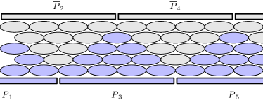
Figure 3: Pulling out local projectors from coarse-grained projectors in a system with $r=8$. Small ellipses are local projectors $P_{i}$. Wide rectangles are coarse-grained $\bar{P}_{\alpha}$.

Notice that $(\Pi_{\text{even}}\Pi_{\text{odd}}\Pi_{\text{even}}\big{)}^{q}=\big{(}\mathop{\rm DL}\nolimits(H)^{\dagger}\mathop{\rm DL}\nolimits(H)\big{)}^{q}$, so that applying the DL on $H$ we may conclude that for any $|\psi^{\perp}\rangle\in V_{gs}^{\perp}$,

$$\big{\|}\bar{\Pi}_{\text{even}}\cdot\bar{\Pi}_{\text{odd}}|\psi^{\perp}\rangle\big{\|}^{2}\leq\left(\frac{1}{\gamma/4+1}\right)^{2\lfloor\frac{r}{4}\rfloor}=1-\operatorname{\Omega}\bigl{(}r\gamma\bigr{)}.$$

Together with (9) this is already sufficient to obtain a lower bound on the spectral gap of $\bar{H}$. To improve the bound to the quadratic dependence on $\gamma$ claimed in the theorem, we follow an idea from LABEL:ref:GH2015-DLAmp of using the Chebyshev polynomial to boost the effect of the DL. For the sake of completeness, we repeat the argument in detail.

Let $A:=\mathop{\rm DL}\nolimits(H)^{\dagger}\mathop{\rm DL}\nolimits(H)=\Pi_{\text{even}}\Pi_{\text{odd}}\Pi_{\text{even}}$. Using Claim 6, for any polynomial $P_{q}$ of degree $q\leq\lfloor\frac{r}{4}\rfloor$ such that $P_{q}(1)=1$, it holds that $\bar{\Pi}_{\text{even}}\cdot\bar{\Pi}_{\text{odd}}=\bar{\Pi}_{\text{even}}\cdot P_{q}(A)\cdot\bar{\Pi}_{\text{odd}}$. By definition, for any $|\psi^{\perp}\rangle\in V_{gs}^{\perp}$, we have $\bar{\Pi}_{\text{odd}}|\psi^{\perp}\rangle\in V_{gs}^{\perp}$ (to see this, multiply from the left by any ground state of $\bar{H}$). Using that $\|\bar{\Pi}_{\text{even}}\|\leq 1$, we conclude

$$\max_{|\psi^{\perp}\rangle}\big{\|}\bar{\Pi}_{\text{even}}\cdot\bar{\Pi}_{\text{odd}}|\psi^{\perp}\rangle\big{\|}$$

$$\ \ \leq\max_{|\psi^{\perp}\rangle}\big{\|}\bar{\Pi}_{\text{even}}\cdot P_{q}(A)\cdot\bar{\Pi}_{\text{odd}}|\psi^{\perp}\rangle\big{\|}$$

$$\ \ \leq\max_{|\psi^{\perp}\rangle}\big{\|}P_{q}(A)|\psi^{\perp}\rangle\big{\|}.$$ (10)

Our goal is therefore to find a polynomial $P_{q}(x)$ that would minimize the RHS of the above inequality. Since $A$ is Hermitian, we may expand $|\psi^{\perp}\rangle$ in a basis of eigenstates of $A$ as $|\psi^{\perp}\rangle=\sum_{\mu}\psi_{\mu}|\mu\rangle$. By definition, $0\leq A\leq\mathbbm{1}$, and so its eigenvalues are in the range $[0,1]$. The $\mu=1$ eigenvalue corresponds to the ground space of $H$, and since $A=\mathop{\rm DL}\nolimits(H)^{\dagger}\mathop{\rm DL}\nolimits(H)$, it follows from the DL that all other eigenvalues of $A$ are upper bounded by $h:=\frac{1}{\gamma/4+1}$. We therefore look for a polynomial $P_{q}(x)$ with $q\leq\lfloor\frac{r}{4}\rfloor$ such that $P_{q}(1)=1$ and $|P(x)|$ is minimal for $x\in[0,h]$. Following the approach of the AGSP-based area-law proofs[21, 26], we choose $P_{q}$ to be a rescaled Chebyshev polynomial of degree $q$ of the first kind. The exact construction is summarized in Lemma 7 given at the end of this section. Substituting $h=\frac{1}{\gamma/4+1}$ in the lemma and noticing that as $\gamma\leq g+1=3$ (see the discussion following Corollary 3 for a justification), it follows that $1-h=1-\frac{1}{\gamma/4+1}\geq\gamma/8$, and consequently for every $x\in[0,h]$,

$$|P_{q}(x)|\leq 2e^{-q\sqrt{\gamma/2}}.$$ (11)

Therefore, $\|P_{q}(A)|\psi^{\perp}\rangle\|\leq 2e^{-q\sqrt{\gamma/2}}$ for every $|\psi^{\perp}\rangle\in V_{gs}^{\perp}$, and combining (9) and (10),

$$\bar{\gamma}\geq\frac{1}{4}-e^{-2q\sqrt{\gamma/2}}.$$

Finally, the theorem is proved by choosing $q=\lfloor\frac{r}{4}\rfloor\geq\frac{r}{4}-1$.  

Lemma 7

Let $0<h<1$, and let $T_{q}(x)$ be the Chebyshev polynomial of the first kind of degree $q$. Define

$$\tilde{P}_{q}(x) :=T_{q}(2\frac{x}{h}-1), P_{q}(x) :=\tilde{P}_{q}(x)/\tilde{P}_{q}(1).$$

Then $P_{q}(1)=1$ and for any $x\in[0,h]$ it holds that $|P_{q}(x)|\leq 2e^{-2q\sqrt{1-h}}$.

• $P_{q}(1)=1$ holds by definition. Using the well-known properties of the Chebyshev polynomial (see, for example, Lemma 4.1 in LABEL:ref:AKLV2013-AL),

  $$|T_{q}(x)| \leq 1, \text{for $|x|\leq 1$},$$

  $$|T_{q}(x)| \geq\frac{1}{2}\exp{\left(2q\sqrt{(|x|-1)/(|x|+1)}\right)}, \text{for $|x|>1$},$$

  it is easy to see that $|\tilde{P}_{q}(1)|\geq\frac{1}{2}e^{2q\sqrt{1-h}}$, and therefore for $x\in[0,h]$ we have $|P_{q}(x)|\leq 2e^{-2q\sqrt{1-h}}$.  

V Summary

We have provided a short proof of the DL which tightens its bound and generalizes it to arbitrary orderings of the local projectors. Using an explicit example, we showed that the new bound is optimal in its dependence on $g$ when $\epsilon_{\phi}\to 0$, up to constant factors. In addition, we have shown how the lemma can be combined with a converse bound to prove that by coarse graining a frustration-free Hamiltonian with a gap $\gamma>0$ to a length scale $\operatorname{O}\bigl{(}\gamma^{-1/2}\bigr{)}$, one obtains a Hamiltonian with a constant spectral gap. It would be interesting to see if, by using the converse to the DL, one can apply the DL to slightly frustrated systems with a constant gap in a controlled manner. If this can be done, it would extend the applicability DL to much broader set of problems, which may benefit from its simplicity with respect to other techniques.