High-Dimensional Regularized Discriminant Analysis

Abstract

Regularized discriminant analysis (RDA), proposed by Friedman (1989), is a widely popular classifier that lacks interpretability and is impractical for high-dimensional data sets. Here, we present an interpretable and computationally efficient classifier called high-dimensional RDA (HDRDA), designed for the small-sample, high-dimensional setting. For HDRDA, we show that each training observation, regardless of class, contributes to the class covariance matrix, resulting in an interpretable estimator that borrows from the pooled sample covariance matrix. Moreover, we show that HDRDA is equivalent to a classifier in a reduced-feature space with dimension approximately equal to the training sample size. As a result, the matrix operations employed by HDRDA are computationally linear in the number of features, making the classifier well-suited for high-dimensional classification in practice. We demonstrate that HDRDA is often superior to several sparse and regularized classifiers in terms of classification accuracy with three artificial and six real high-dimensional data sets. Also, timing comparisons between our HDRDA implementation in the sparsediscrim R package and the standard RDA formulation in the klaR R package demonstrate that as the number of features increases, the computational runtime of HDRDA is drastically smaller than that of RDA.

1 Introduction

In this paper, we consider the classification of small-sample, high-dimensional data, where the number of features $p$ exceeds the training sample size $N$. In this setting, well-established classifiers, such as linear discriminant analysis (LDA) and quadratic discriminant analysis (QDA), become incalculable because the class and pooled covariance matrix estimators are singular (Murphy, 2012; Bouveyron, Girard, and Schmid, 2007; Mkhadri, Celeux, and Nasroallah, 1997). To improve the accuracy of the estimation of the class covariance matrices estimated in the QDA classifier and to ensure that the covariance matrix estimators are nonsingular, Friedman (1989) proposed the regularized discriminant analysis (RDA) classifier by incorporating a weighted average of the pooled sample covariance matrix and the class sample covariance matrix. To further improve the accuracy of the estimation of the class covariance matrix and to stabilize its inverse, Friedman (1989) also included a regularization component by shrinking the covariance matrix estimator towards the identity matrix, which yields a nonsingular estimator following the well-known ridge-regression approach of Hoerl and Kennard (1970). Despite its popularity, the “borrowing” operation employed in the RDA classifier lacks interpretability (Bensmail and Celeux, 1996). Furthermore, the RDA classifier is impractical for high-dimensional data sets because it computes the inverse and determinant of the covariance matrices for each class. Both matrix calculations are computationally expensive because the number of operations grows at a polynomial rate in the number of features. Moreover, the model selection of the RDA classifier’s two tuning parameters is computationally burdensome because the matrix inverse and determinant of each class covariance matrix are computed across multiple cross-validation folds for each candidate tuning-parameter pair.

Here, we present the high-dimensional RDA (HDRDA) classifier, which is intended for the case when $p>N$ . We reparameterize the RDA classifier similar to that of Hastie, Tibshirani, and Friedman (2008) and Halbe and Aladjem (2007) and employ a biased covariance-matrix estimator that partially pools the individual sample covariance matrices from the QDA classifier with the pooled sample covariance matrix from the LDA classifier. We then shrink the resulting covariance-matrix estimator towards a scaled identity matrix to ensure positive definiteness. We show that the pooling parameter in the HDRDA classifier determines the contribution of each training observation to the estimation of each class covariance matrix, enabling interpretability that has been previously lacking with the RDA classifier (Bensmail and Celeux, 1996). Our parameterization differs from that of Hastie, Tibshirani, and Friedman (2008) and that of Halbe and Aladjem (2007) in that our formulation allows the flexibility of various covariance-matrix estimators proposed in the literature, including a variety of ridge-like estimators, such as the one proposed by Srivastava and Kubokawa (2007).

Next, we establish that the matrix operations corresponding to the null space of the pooled sample covariance matrix are redundant and can be discarded from the HDRDA decision rule without loss of classificatory information when we apply reasoning similar to that of Ye and Wang (2006). As a result, we achieve a substantial reduction in dimension such that the matrix operations used in the HDRDA classifier are computationally linear in the number of features. Furthermore, we demonstrate that the HDRDA decision rule is invariant to adjustments to the approximately $p-N$ zero eigenvalues, so that the decision rule in the original feature space is equivalent to a decision rule in a lower dimension, such that matrix inverses and determinants of relatively small matrices can be rapidly computed. Finally, we show that several shrinkage methods that are special cases of the HDRDA classifier have no effect on the approximately $p-N$ zero eigenvalues of the covariance-matrix estimators when $p>N$. Such techniques include work from Srivastava and Kubokawa (2007), Rao and Mitra (1971), and other methods studied by Ramey and Young (2013) and Xu, Brock, and Parrish (2009).

We also provide an efficient algorithm along with pseudocode to estimate the HDRDA classifier’s tuning parameters in a grid search via cross-validation. Timing comparisons between our HDRDA implementation in the sparsediscrim R package available on CRAN and the standard RDA formulation in the klaR R package demonstrate that as the number of features increases, the computational runtime of the HDRDA classifier is drastically smaller than that of RDA. In fact, when $p=5000$, we show that the HDRDA classifier is 502.786 times faster on average than the RDA classifier. In this scenario, the HDRDA classifier’s model selection requires 2.979 seconds on average, while that of the RDA classifier requires 24.933 minutes on average.

Finally, we study the classification performance of the HDRDA classifier on six real high-dimensional data sets along with a simulation design that generalizes the experiments initially conducted by Guo et al. (2007). We demonstrate that the HDRDA classifier often attains superior classification accuracy to several recent classifiers designed for small-sample, high-dimensional data from Tong, Chen, and Zhao (2012), Witten and Tibshirani (2011), Pang, Tong, and Zhao (2009), and Guo et al. (2007). We also include as a benchmark the random forest from Breiman (2001) because Fernández-Delgado, Cernadas, Barro, and Amorim (2014) have concluded that the random forest is often superior to other classifiers in benchmark studies. We show that our proposed classifier is competitive and often outperforms the random forest in terms of classification accuracy in the small-sample, high-dimensional setting.

The remainder of this paper is organized as follows. In Section 2 we introduce the classification problem and necessary notation to describe our contributions. In Section 3 we present the HDRDA classifier along with its interpretation. In Section 4, we provide properties of the HDRDA classifier and a computationally efficient model-selection procedure. In Section 5, we compare the model-selection timings of the HDRDA and RDA classifiers. In Section 6 we describe our simulation studies of artificial and real data sets and examine the experimental results. We conclude with a brief discussion in Section 7.

2 Preliminaries

2.1 Notation

To facilitate our discussion of covariance-matrix regularization and high-dimensional classification, we require the following notation. Let $\mathbb{R}_{a\times b}$ denote the matrix space of all $a\times b$ matrices over the real field $\mathbb{R}$. Denote by $\bm{I}_{m}$ the $m\times m$ identity matrix, and let $\bm{0}_{m\times p}$ be the $m\times p$ matrix of zeros, such that $\bm{0}_{m}$ is understood to denote $\bm{0}_{m\times m}$. Define $\bm{1}_{m}\in\mathbb{R}_{m\times 1}$ as a vector of ones. Let $\bm{A}^{T}$, $\bm{A}^{+}$, and $\mathcal{N}(\bm{A})$ denote the transpose, the Moore-Penrose pseudoinverse, and the null space of $\bm{A}\in\mathbb{R}_{m\times p}$, respectively. Denote by $\mathbb{R}_{p\times p}^{>}$ the cone of real $p\times p$ positive-definite matrices. Similarly, let $\mathbb{R}_{p\times p}^{\geq}$ denote the cone of real $p\times p$ positive-semidefinite matrices. Let $V^{\perp}$ denote the orthogonal complement of a vector space $V\subset\mathbb{R}_{p\times 1}$. For $c\in\mathbb{R}$, let $c^{+}=1/c$ if $c\neq 0$ and $0$ otherwise.

2.2 Discriminant Analysis

In discriminant analysis we wish to assign an unlabeled vector $\bm{x}\in\mathbb{R}_{p\times 1}$ to one of $K$ unique, known classes by constructing a classifier from $N$ training observations. Let $\bm{x}_{i}=(x_{i1},\ldots,x_{ip})\in\mathbb{R}_{p\times 1}$ be the $i$th observation $(i=1,\ldots,N)$ with true, unique membership $y_{i}\in\{\omega_{1},\ldots,\omega_{K}\}$. Denote by $n_{k}$ the number of training observations realized from class $k$, such that $\sum_{k=1}^{K}n_{k}=N$. We assume that $(\bm{x}_{i},y_{i})$ is a realization from a mixture distribution $p(\bm{x})=\sum_{k=1}^{K}p(\bm{x}|\omega_{k})p(\omega_{k})$, where $p(\bm{x}|\omega_{k})$ is the probability density function (PDF) of the $k$th class and $p(\omega_{k})$ is the prior probability of class membership of the $k$th class. We further assume $p(\omega_{k})=p(\omega_{l})$, $1\leq k,l\leq K$, $k\neq l$.

The QDA classifier is the optimal Bayesian decision rule with respect to a $0-1$ loss function when $p(\bm{x}|\omega_{k})$ is the PDF of the multivariate normal distribution with known mean vectors $\bm{\mu}_{k}\in\mathbb{R}_{p\times 1}$ and known covariance matrices $\bm{\Sigma}_{k}\in\mathbb{R}_{p\times p}^{>}$, $k=1,2,\ldots,K$. Because $\bm{\mu}_{k}$ and $\bm{\Sigma}_{k}$ are typically unknown, we assign an unlabeled observation $\bm{x}$ to class $\omega_{k}$ with the sample QDA classifier

$$D_{QDA}(\bm{x})=\operatorname*{arg\,min}_{k}(\bm{x}-\bar{\bm{x}}_{k})^{T}\widehat{\bm{\Sigma}}_{k}^{-1}(\bm{x}-\bar{\bm{x}}_{k})+\log|\widehat{\bm{\Sigma}}_{k}|,$$ (1)

where $\bar{\bm{x}}_{k}$ and $\widehat{\bm{\Sigma}}_{k}$ are the maximum-likelihood estimators (MLEs) of $\bm{\mu}_{k}$ and $\bm{\Sigma}_{k}$, respectively. If we assume further that $\bm{\Sigma}_{k}=\bm{\Sigma}$, $k=1,\ldots,K$, then the pooled sample covariance matrix $\widehat{\bm{\Sigma}}$ is substituted for $\widehat{\bm{\Sigma}}_{k}$ in (1), where

$$\widehat{\bm{\Sigma}}=N^{-1}\sum_{k=1}^{K}n_{k}\widehat{\bm{\Sigma}}_{k}$$ (2)

is the MLE for $\bm{\Sigma}$. Here, (1) reduces to the sample LDA classifier. We omit the log-determinant because it is constant across the $K$ classes.

The smallest eigenvalues of $\widehat{\bm{\Sigma}}_{k}$ and the directions associated with their eigenvectors can highly influence the classifier in (1). In fact, the eigenvalues of $\widehat{\bm{\Sigma}}_{k}$ are well-known to be biased if $p\geq n_{k}$ such that the smallest eigenvalues are underestimated (Seber, 2004). Moreover, if $p>n_{k}$, then rank$(\widehat{\bm{\Sigma}}_{k})\leq n_{k}$, which implies that at least $p-n_{k}$ eigenvalues of $\widehat{\bm{\Sigma}}_{k}$ are zero. Furthermore, although more feature information is available to discriminate among the $K$ classes, if $p>n_{k}$, (1) is incalculable because $\widehat{\bm{\Sigma}}_{k}^{-1}$ does not exist.

Several regularization methods, such as the methods considered by Xu et al. (2009), Guo et al. (2007), and Mkhadri (1995), have been proposed in the literature to adjust the eigenvalues of $\widehat{\bm{\Sigma}}_{k}$ so that (1) is calculable and provides reduced variability for $\widehat{\bm{\Sigma}}_{k}^{-1}$. A common form of the covariance-matrix regularization applies a shrinkage factor $\gamma>0$, so that

$$\widehat{\bm{\Sigma}}_{k}(\gamma)=\widehat{\bm{\Sigma}}_{k}+\gamma\bm{I}_{p},$$ (3)

similar to a method employed in ridge regression (Hoerl and Kennard, 1970). Equation (3) effectively shrinks the sample covariance matrix $\widehat{\bm{\Sigma}}_{k}$ toward $\bm{I}_{p}$, thereby increasing the eigenvalues of $\widehat{\bm{\Sigma}}_{k}$ by $\gamma$. Specifically, the zero eigenvalues are replaced with $\gamma$, so that (3) is positive definite. For additional covariance-matrix regularization methods, see Ramey and Young (2013), Xu et al. (2009), and Ye and Ji (2009).

3 High-Dimensional Regularized Discriminant Analysis

Here, we define the HDRDA classifier by first formulating the covariance-matrix estimator $\widehat{\bm{\Sigma}}_{k}(\lambda)$ and demonstrating its clear interpretation as a linear combination of the crossproducts of the training observations centered by their respective class sample means. We define the convex combination

$$\widehat{\bm{\Sigma}}_{k}(\lambda)\coloneqq(1-\lambda)\widehat{\bm{\Sigma}}_{k}+\lambda\widehat{\bm{\Sigma}},\quad k=1,\ldots,K,$$ (4)

where $\lambda\in[0,1]$ is the pooling parameter. By rewriting (4) in terms of the observations $\bm{x}_{i}$, $i=1,\ldots,N$, each centered by its class sample mean, we attain a clear interpretation of $\widehat{\bm{\Sigma}}_{k}(\lambda)$. That is,

$$\widehat{\bm{\Sigma}}_{k}(\lambda) =\left(1-\lambda+\frac{\lambda n_{k}}{N}\right)\widehat{\bm{\Sigma}}_{k}+\frac{\lambda}{N}\sum_{\begin{subarray}{c}k^{\prime}=1\\ k^{\prime}\neq k\end{subarray}}^{K}n_{k^{\prime}}\widehat{\bm{\Sigma}}_{k^{\prime}}$$

$$=\left(\frac{1-\lambda}{n_{k}}+\frac{\lambda}{N}\right)\sum_{i=1}^{N}I(y_{i}=k)\bm{x}_{i}\bm{x}_{i}^{T}+\frac{\lambda}{N}\sum_{i=1}^{N}I(y_{i}\neq k)\bm{x}_{i}\bm{x}_{i}^{T}$$

$$=\sum_{i=1}^{N}c_{ik}(\lambda)\bm{x}_{i}\bm{x}_{i}^{T},$$ (5)

where $c_{ik}(\lambda)=\lambda N^{-1}+(1-\lambda)n_{k}^{-1}I(y_{i}=k)$. From (5), we see that $\lambda$ weights the contribution of each of the $N$ observations in estimating $\bm{\Sigma}_{k}$ from all $K$ classes rather than using only the $n_{k}$ observations from a single class. As a result, we can interpret (5) as a covariance-matrix estimator that borrows from $\widehat{\bm{\Sigma}}$ in (2) to estimate $\bm{\Sigma}_{k}$.

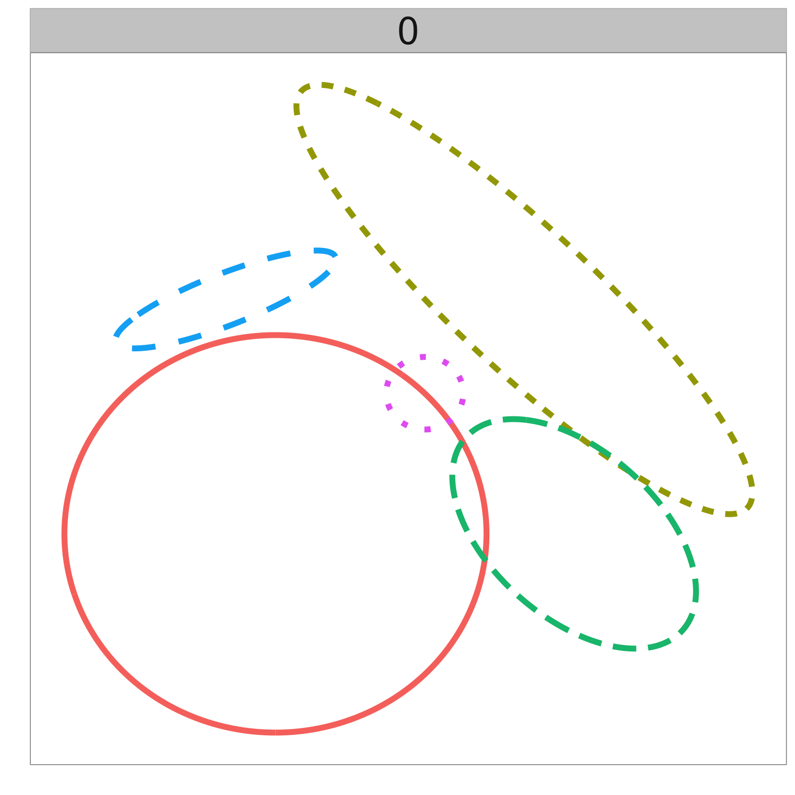
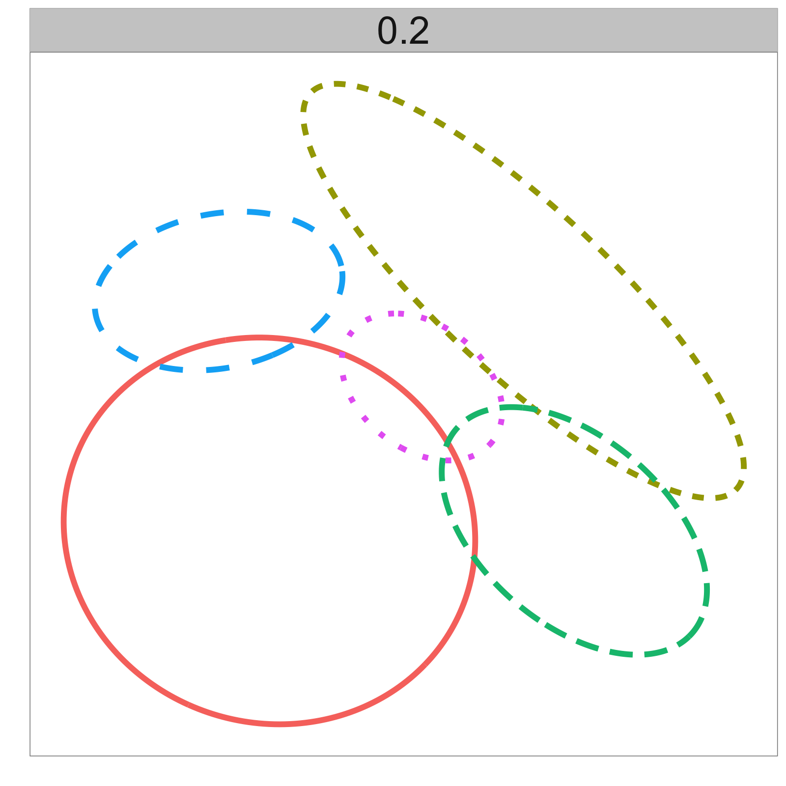
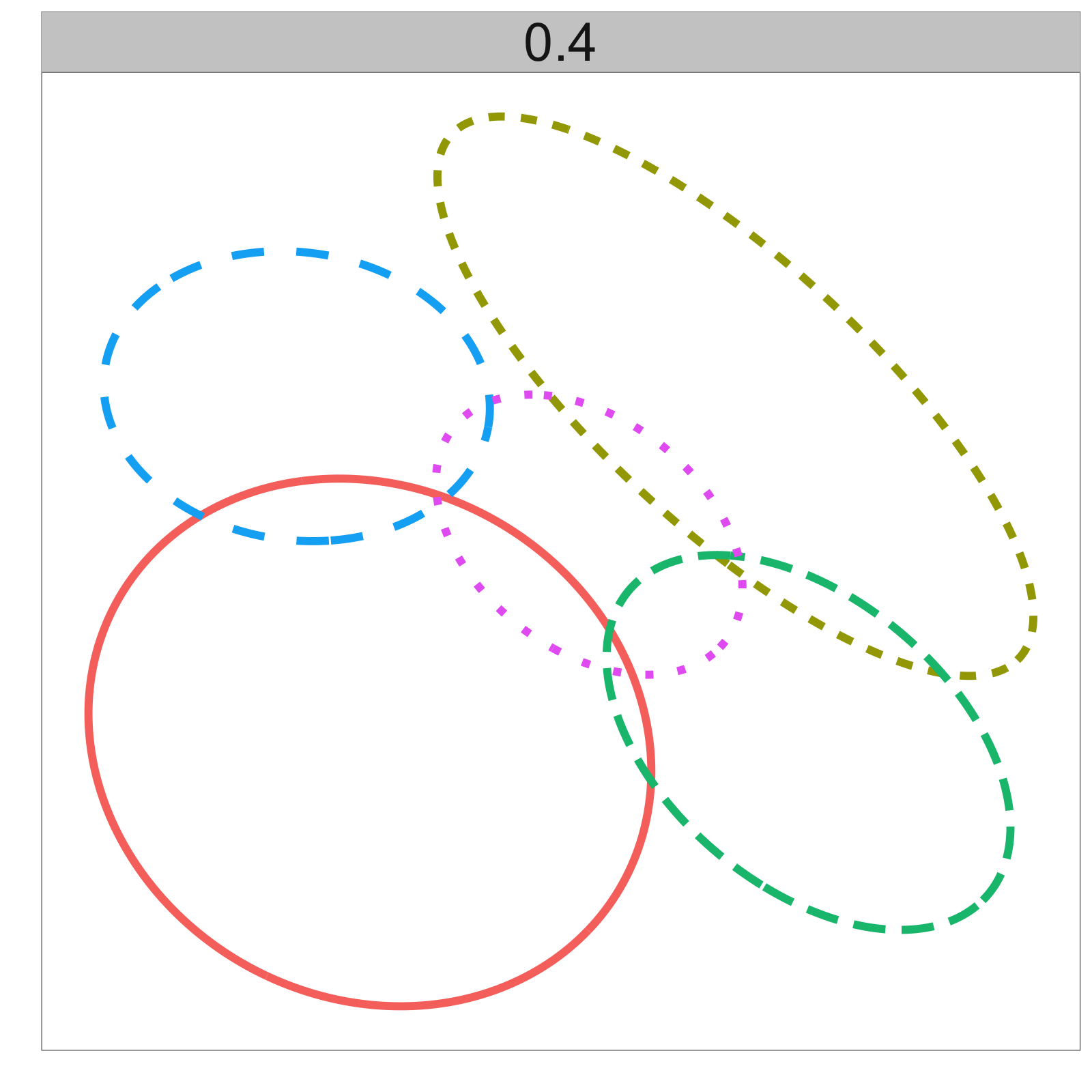
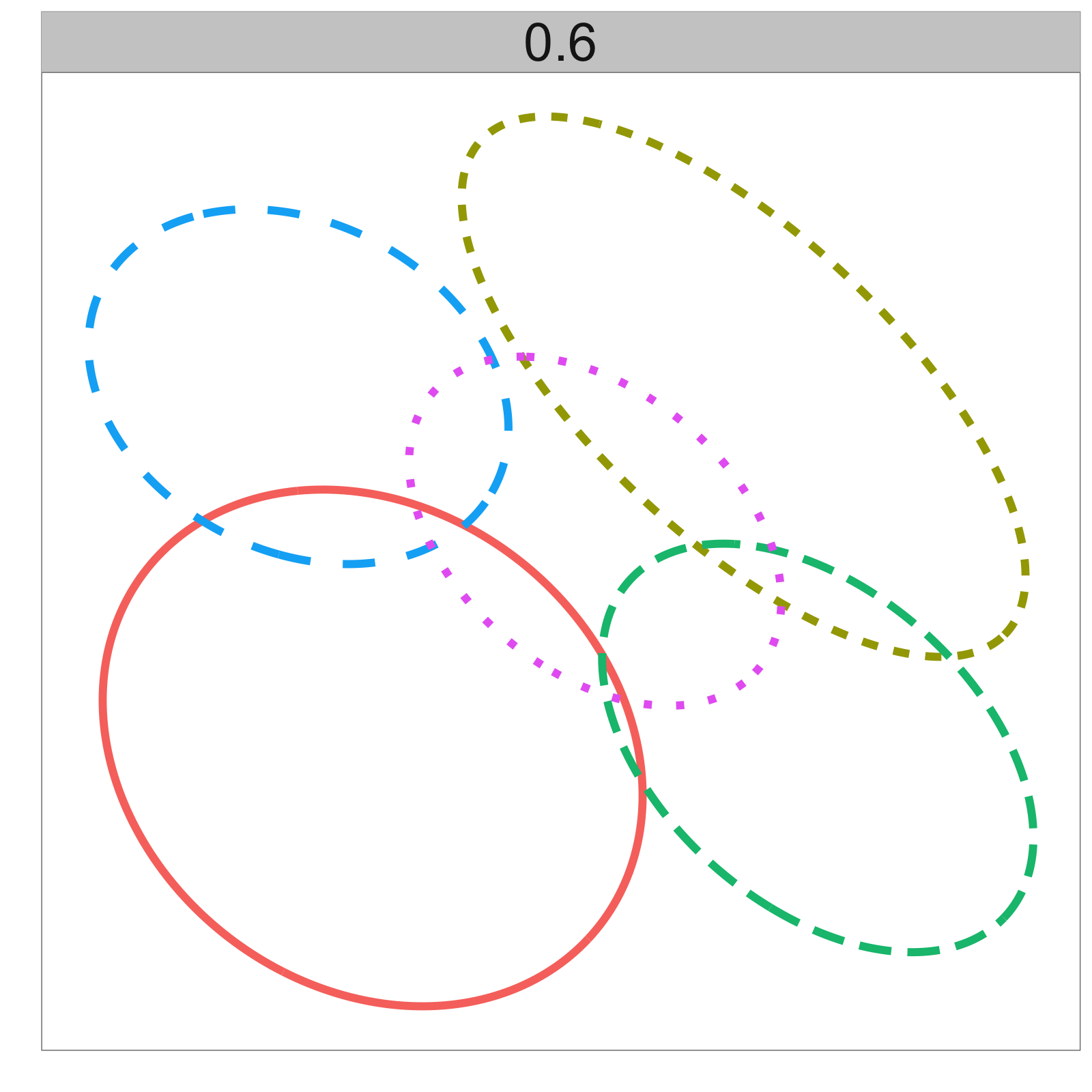
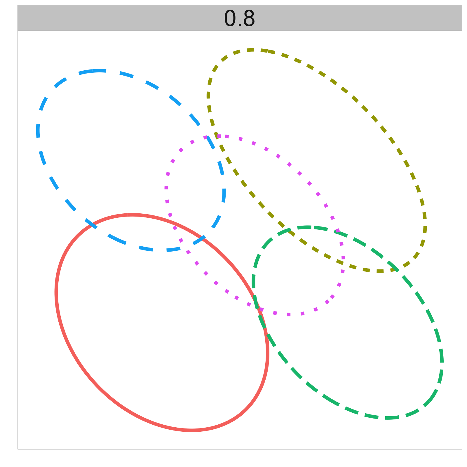
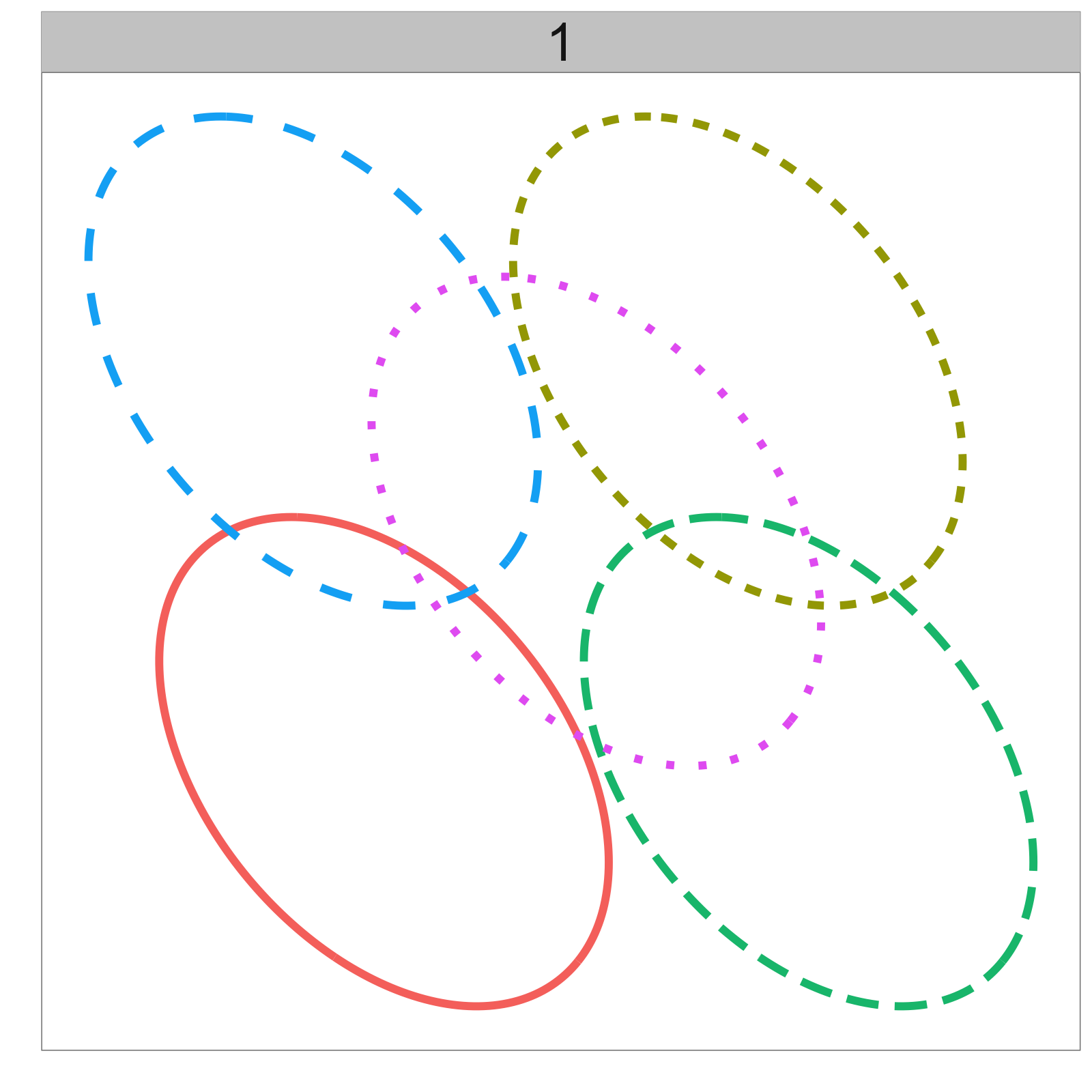
Figure 1: Contours of five multivariate normal populations as a function of the pooling parameter $\lambda$.

In Figure 1 we plot the contours of five multivariate normal populations for $\lambda=0$ with unequal covariance matrices. As $\lambda$ approaches 1, the contours become more similar, resulting in identical contours for $\lambda=1$. Below, we show that the pooling operation is advantageous in increasing the rank of each $\widehat{\bm{\Sigma}}_{k}(\lambda)$ from rank$(\widehat{\bm{\Sigma}}_{k})$ to rank$(\widehat{\bm{\Sigma}})$ for $0<\lambda\leq 1$. Notice that if $\lambda=0$, then the observations from the remaining $K-1$ classes do not contribute to the estimation of $\bm{\Sigma}_{k}$, corresponding to $\widehat{\bm{\Sigma}}_{k}$. Furthermore, if $\lambda=1$, the weights $c_{ik}(\lambda)$ in (5) reduce to $1/N$, corresponding to $\widehat{\bm{\Sigma}}$. For brevity, when $\lambda=1$, we define $\bm{X}=[\sqrt{c_{1k}(1)}\bm{x}_{1}^{T},\ldots,\sqrt{c_{Nk}(1)}\bm{x}_{N}^{T}]^{T}$ such that $\widehat{\bm{\Sigma}}=N^{-1}\bm{X}^{T}\bm{X}$. Similarly, for $\lambda=0$, we define $\bm{X}_{k}=[\sqrt{c_{1k}(0)}\bm{x}_{1}^{T},\ldots,\sqrt{c_{Nk}(0)}\bm{x}_{N}^{T}]^{T}$ such that $\widehat{\bm{\Sigma}}_{k}=n_{k}^{-1}\bm{X}_{k}^{T}\bm{X}_{k}$.

$$\left[\text{Insert Figure \ref{fig:hdrda-contours} approximately here }\right]$$

As we have discussed above, several eigenvalue adjustment methods have been proposed that increase eigenvalues (approximately) equal to 0. To further improve the estimation of $\bm{\Sigma}_{k}$ and to stabilize the estimator’s inverse, we define the eigenvalue adjustment of (4) as

$$\tilde{\bm{\Sigma}}_{k}\coloneqq\alpha_{k}\widehat{\bm{\Sigma}}_{k}(\lambda)+\gamma\bm{I}_{p},$$ (6)

where $\alpha_{k}\geq 0$ and $\gamma\geq 0$ is an eigenvalue-shrinkage constant. Thus, the pooling parameter $\lambda$ controls the amount of estimation information borrowed from $\widehat{\bm{\Sigma}}$ to estimate $\bm{\Sigma}_{k}$, and the shrinkage parameter $\gamma$ determines the degree of eigenvalue shrinkage. The choice of $\alpha_{k}$ allows for a flexible formulation of covariance-matrix estimators. For instance, if $\alpha_{k}=1$, $k=1,\ldots,K$, then (6) resembles (3). Similarly, if $\alpha_{k}=1-\gamma$, then (6) has a form comparable to the RDA classifier from Friedman (1989). Substituting (6) into (1), we define the HDRDA classifier as

$$D_{HDRDA}(\bm{x})=\operatorname*{arg\,min}_{k}(\bm{x}-\bar{\bm{x}}_{k})^{T}\tilde{\bm{\Sigma}}_{k}^{+}(\bm{x}-\bar{\bm{x}}_{k})+\log|\tilde{\bm{\Sigma}}_{k}|.$$ (7)

For $\gamma>0$, $\tilde{\bm{\Sigma}}_{k}$ is nonsingular such that $\tilde{\bm{\Sigma}}_{k}^{-1}$ can be substituted for $\tilde{\bm{\Sigma}}_{k}^{+}$ in (7). If $\gamma=0$, we explicitly set $|\tilde{\bm{\Sigma}}_{k}|$ equal to the product of the positive eigenvalues of $\tilde{\bm{\Sigma}}_{k}$. Following Friedman (1989), we select $\lambda$ and $\gamma$ from a grid of candidate models via cross-validation (Hastie et al., 2008). We provide an implementation of (7) in the hdrda function contained in the sparsediscrim R package, which is available on CRAN.

The choice of $\alpha_{k}$ in (6) is one of convenience and allows the flexibility of various covariance-matrix estimators proposed in the literature. In practice, we generally are not interested in estimating $\alpha_{k}$ because the estimation of $K$ additional tuning parameters via cross-validation is counterproductive to our goal of computational efficiency. For appropriate values of $\alpha_{k}$, the HDRDA covariance-matrix estimator includes or resembles a large family of estimators. Notice that if $\alpha_{k}=1$ and $\lambda=1$, (6) is equivalent to the standard ridge-like covariance-matrix estimator in (3). Other estimators proposed in the literature can be obtained when one selects $\gamma$ accordingly. For instance, with $\gamma=\text{tr}\{\widehat{\bm{\Sigma}}\}/\min(N,p)$, we obtain the estimator from Srivastava and Kubokawa (2007).

When $\alpha_{k}=1-\gamma$, (6) resembles the biased covariance-matrix estimator

$$\widehat{\bm{\Sigma}}_{k}(\lambda,\gamma)=(1-\gamma)\widehat{\bm{\Sigma}}_{k}^{(RDA)}(\lambda)+\gamma\frac{\text{tr}\left\{\widehat{\bm{\Sigma}}_{k}^{(RDA)}(\lambda)\right\}}{p}\bm{I}_{p}$$ (8)

employed in the RDA classifier, where $\widehat{\bm{\Sigma}}_{k}^{(RDA)}(\lambda)$ is a pooled estimator of $\bm{\Sigma}_{k}$ and $\gamma\in[0,1]$ is a regularization parameter that controls the shrinkage of (8) towards $\bm{I}_{p}$ weighted by the average of the eigenvalues of $\widehat{\bm{\Sigma}}_{k}^{(RDA)}(\lambda)$. Despite the similarity of (8) to the HDRDA covariance-matrix estimator in (6), the RDA classifier is impractical for high-dimensional data because the inverse and determinant of (8) must be calculated when substituted into (1). Furthermore, (8) has no clear interpretation.

4 Properties of the HDRDA Classifier

Next, we establish properties of the covariance-matrix estimator and the decision rule employed in the HDRDA classifier. By doing so, we demonstrate that (7) lends itself to a more efficient calculation. We decompose (7) into a sum of two components, where the first summand consists of matrix operations applied to low-dimensional matrices and the second summand corresponds to the null space of $\widehat{\bm{\Sigma}}$ in (2). We show that the matrix operations performed on the null space of $\widehat{\bm{\Sigma}}$ yield constant quadratic forms across all classes and can be omitted. For $p\gg N$, the constant component involves determinants and inverses of high-dimensional matrices, and by ignoring these calculations, we achieve a substantial reduction in computational costs. Furthermore, a byproduct is that adjustments to the associated eigenvalues have no effect on (7). Lastly, we utilize the singular value decomposition to efficiently calculate the eigenvalue decomposition of $\widehat{\bm{\Sigma}}$, further reducing the computational costs of the HDRDA classifier.

First, we require the following relationship regarding the null spaces of $\widehat{\bm{\Sigma}}_{k}(\lambda)$, $\widehat{\bm{\Sigma}}$, and $\widehat{\bm{\Sigma}}_{k}$.

Lemma 1.

Let $\widehat{\bm{\Sigma}}_{k}$ and $\widehat{\bm{\Sigma}}$ be the MLEs of $\bm{\Sigma}_{k}$ and $\bm{\Sigma}$, respectively. Let $\widehat{\bm{\Sigma}}_{k}(\lambda)$ be defined as in (4). Then, $\mathcal{N}\{\widehat{\bm{\Sigma}}_{k}(\lambda)\}\subset\mathcal{N}(\widehat{\bm{\Sigma}})\subset\mathcal{N}(\widehat{\bm{\Sigma}}_{k})$, $k=1,\ldots,K$.

Proof.

Let $\bm{z}\in\mathcal{N}\{\widehat{\bm{\Sigma}}_{k}(\lambda)\}$ for some $k=1,\ldots,K$. Hence, $0=\bm{z}^{T}\widehat{\bm{\Sigma}}_{k}(\lambda)\bm{z}=(1-\lambda)\bm{z}^{T}\widehat{\bm{\Sigma}}_{k}\bm{z}+\lambda\bm{z}^{T}\widehat{\bm{\Sigma}}\bm{z}$. Because $\widehat{\bm{\Sigma}}_{k},\widehat{\bm{\Sigma}}\in\mathbb{R}_{p\times p}^{\geq}$, we have $\bm{z}\in\mathcal{N}(\widehat{\bm{\Sigma}})$ and $\bm{z}\in\mathcal{N}(\widehat{\bm{\Sigma}}_{k})$. In particular, we have that $\mathcal{N}\{\widehat{\bm{\Sigma}}_{k}(\lambda)\}\subset\mathcal{N}(\widehat{\bm{\Sigma}})$. Now, suppose $\bm{z}\in\mathcal{N}(\widehat{\bm{\Sigma}})$. Similarly, we have that $0=\bm{z}^{T}\widehat{\bm{\Sigma}}\bm{z}=N^{-1}\sum_{k=1}^{K}n_{k}\bm{z}^{T}\widehat{\bm{\Sigma}}_{k}\bm{z}$, which implies that $\bm{z}\in\mathcal{N}(\widehat{\bm{\Sigma}}_{k})$ because $\widehat{\bm{\Sigma}}_{k}\in\mathbb{R}_{p\times p}^{\geq}$. Therefore, $\mathcal{N}(\widehat{\bm{\Sigma}})\subset\mathcal{N}(\widehat{\bm{\Sigma}}_{k})$. ∎

In Lemma 2 below, we derive an alternative expression for $\tilde{\bm{\Sigma}}_{k}$ in terms of the matrix of eigenvectors of $\widehat{\bm{\Sigma}}$. Let $\widehat{\bm{\Sigma}}=\bm{U}\bm{D}\bm{U}^{T}$ be the eigendecomposition of $\widehat{\bm{\Sigma}}$ such that $\bm{D}\in\mathbb{R}_{p\times p}^{\geq}$ is the diagonal matrix of eigenvalues of $\widehat{\bm{\Sigma}}$ with

$$\bm{D}=\begin{bmatrix}\bm{D}_{q}&\bm{0}\\ \bm{0}&\bm{0}_{p-q}\end{bmatrix},$$

$\bm{D}_{q}\in\mathbb{R}_{q\times q}^{>}$ is the diagonal matrix consisting of the positive eigenvalues of $\widehat{\bm{\Sigma}}$, the columns of $\bm{U}\in\mathbb{R}_{p\times p}$ are the corresponding orthonormal eigenvectors of $\widehat{\bm{\Sigma}}$, and rank$(\widehat{\bm{\Sigma}})=q$. Then, we partition $\bm{U}=(\bm{U}_{1},\bm{U}_{2})$ such that $\bm{U}_{1}\in\mathbb{R}_{p\times q}$ and $\bm{U}_{2}\in\mathbb{R}_{p\times(p-q)}$.

Lemma 2.

Let $\widehat{\bm{\Sigma}}=\bm{U}\bm{D}\bm{U}^{T}$ be the eigendecomposition of $\widehat{\bm{\Sigma}}$ as above, and suppose that rank$(\widehat{\bm{\Sigma}})=q\leq p$. Then, we have

$$\tilde{\bm{\Sigma}}_{k} =\bm{U}\begin{bmatrix}\bm{W}_{k}&\bm{0}\\ \bm{0}&\gamma\bm{I}_{p-q}\end{bmatrix}\bm{U}^{T},\quad k=1,\ldots,K,$$ (9)

where

$$\bm{W}_{k} =\alpha_{k}\{(1-\lambda)\bm{U}_{1}^{T}\widehat{\bm{\Sigma}}_{k}\bm{U}_{1}+\lambda\bm{D}_{q}\}+\gamma\bm{I}_{q}.$$ (10)

Proof.

From Lemma 1, the columns of $\bm{U}_{2}$ span the null space of $\widehat{\bm{\Sigma}}_{k}$, which implies that $\widehat{\bm{\Sigma}}_{k}\bm{U}_{2}=\bm{0}_{p\times(p-q)}$. Hence,

$$\bm{U}^{T}\widehat{\bm{\Sigma}}_{k}\bm{U}=\begin{bmatrix}\bm{U}_{1}^{T}\widehat{\bm{\Sigma}}_{k}\bm{U}_{1}&\bm{0}\\ \bm{0}&\bm{0}_{p-q}\end{bmatrix},\quad k=1,\ldots,K.$$

Thus, $\bm{U}^{T}\tilde{\bm{\Sigma}}_{k}\bm{U}=\alpha_{k}\{(1-\lambda)\bm{U}^{T}\widehat{\bm{\Sigma}}_{k}\bm{U}+\lambda\bm{D}\}+\gamma\bm{I}_{p}$, and (9) holds because $\bm{U}$ is orthogonal. ∎

As an immediate consequence of Lemma 2, we have the following corollary.

Corollary 1.

Let $\widehat{\bm{\Sigma}}_{k}(\lambda)$ be defined as in (4). Then, for $\lambda\in(0,1]$, rank$\{\widehat{\bm{\Sigma}}_{k}(\lambda)\}=q$, $k=1,\ldots,K$.

Proof.

The proof follows when we set $\gamma=0$ in Lemma 2. ∎

Thus, by incorporating each $\bm{x}_{i}$ into the estimation of $\bm{\Sigma}_{k}$, we increase the rank of $\widehat{\bm{\Sigma}}_{k}(\lambda)$ to $q\approx N$ if $\lambda\neq 0$. Next, we provide an essential result that enables us to prove that (7) is invariant to adjustments to the eigenvalues of $\tilde{\bm{\Sigma}}_{k}$ corresponding to the null space of $\widehat{\bm{\Sigma}}$.

Lemma 3.

Let $\bm{U}_{2}$ be defined as above. Then, for all $\bm{x}\in\mathbb{R}_{p\times 1}$, $\bm{U}_{2}^{T}(\bm{x}-\bar{\bm{x}}_{k})=\bm{U}_{2}^{T}(\bm{x}-\bar{\bm{x}}_{k^{\prime}})$, $1\leq k,k^{\prime}\leq K$, where $k\neq k^{\prime}$.

Proof.

Let $\bm{x}\in\mathbb{R}_{p\times 1}$, and suppose that $1\leq k,k^{\prime}\leq K$. Recall that $\bm{U}_{2}\in\mathcal{N}(\widehat{\bm{\Sigma}})$, which implies that $\bm{U}_{2}^{T}\in\mathcal{C}(\widehat{\bm{\Sigma}})^{\perp}$ (Kollo and von Rosen, 2005, Lemma 1.2.5). Now, because $\bm{x}_{i}\in\mathcal{C}(\widehat{\bm{\Sigma}})$ $(i=1,\ldots,N)$, $\bm{U}_{2}^{T}\bm{x}_{i}=\bm{0}_{p-q}$. Hence, $\bm{0}_{p-q}=\sum_{i=1}^{N}\beta_{i}\bm{U}_{2}^{T}\bm{x}_{i}=\bm{U}_{2}^{T}(\bar{\bm{x}}_{k}-\bar{\bm{x}}_{k^{\prime}})$, where $\beta_{i}=(n_{k}n_{k^{\prime}})^{-1}\{I(y_{i}=k)n_{k^{\prime}}-I(y_{i}=k^{\prime})n_{k}\}$. Therefore, $\bm{U}_{2}^{T}(\bm{x}-\bar{\bm{x}}_{k})=\bm{U}_{2}^{T}(\bm{x}-\bar{\bm{x}}_{k^{\prime}})$. ∎

We now present our main result, where we decompose (7) and show that the term requiring the largest computational costs does not contribute to the classification of an unlabeled observation performed using Lemma 3. Hence, we reduce (7) to an equivalent, more computationally efficient decision rule.

Theorem 1.

Let $\tilde{\bm{\Sigma}}_{k}$ and $\bm{W}_{k}$ be defined as in (9) and (10), respectively, and let $\bm{U}_{1}$ be defined as above. Then, the decision rule in (7) is equivalent to

$$D_{HDRDA}(\bm{x}) =\operatorname*{arg\,min}_{k}(\bm{x}-\bar{\bm{x}}_{k})^{T}\bm{U}_{1}\bm{W}_{k}^{-1}\bm{U}_{1}^{T}(\bm{x}-\bar{\bm{x}}_{k})+\log|\bm{W}_{k}|.$$ (11)

Proof.

From (9), we have that

$$\tilde{\bm{\Sigma}}_{k}^{+}=\bm{U}\begin{bmatrix}\bm{W}_{k}^{-1}&\bm{0}\\ \bm{0}&\gamma^{+}\bm{I}_{p-q}\end{bmatrix}\bm{U}^{T}$$

and $|\tilde{\bm{\Sigma}}_{k}|=\gamma^{p-q}|\bm{W}_{k}|$, $k=1,\ldots,K$. Therefore, for all $\bm{x}\in\mathbb{R}_{p\times 1}$, we have that

$$(\bm{x}-\bar{\bm{x}}_{k})^{T}\tilde{\bm{\Sigma}}_{k}^{+}(\bm{x}-\bar{\bm{x}}_{k})+\log|\tilde{\bm{\Sigma}}_{k}| =(\bm{x}-\bar{\bm{x}}_{k})^{T}\bm{U}_{1}\bm{W}_{k}^{-1}\bm{U}_{1}^{T}(\bm{x}-\bar{\bm{x}}_{k})$$

$$+\gamma^{+}(\bm{x}-\bar{\bm{x}}_{k})^{T}\bm{U}_{2}\bm{U}_{2}^{T}(\bm{x}-\bar{\bm{x}}_{k})+\log|\bm{W}_{k}|$$

$$+(p-q)\log\gamma.$$

Because $\gamma$ is constant for $k=1,\ldots,K$, we can omit the $(p-q)\log\gamma$ term and particularly avoid the calculation of $\log 0$ for $\gamma=0$. Then, the proof follows from Lemma 3 because $\bm{U}_{2}^{T}(\bm{x}-\bar{\bm{x}}_{k})$ is constant for $k=1,\ldots,K$. ∎

Using Theorem 1, we can avoid the time-consuming inverses and determinants of $p\times p$ covariance matrices in (7) and instead calculate these same operations on $\bm{W}_{k}\in\mathbb{R}_{q\times q}$ in (11). The substantial computational improvements arise because our proposed classifier in (7) is invariant to the term $\bm{U}_{2}$, thus yielding an equivalent classifier in (11) with a substantial reduction in computational complexity. Here, we demonstrate that the computational efficiency in calculating the inverse and determinant of $\bm{W}_{k}$ can be further improved via standard matrix operations when we show that the inverses and determinants of $\bm{W}_{k}$ can be performed on matrices of size $n_{k}\times n_{k}$.

Proposition 1.

Let $\bm{W}_{k}$ be defined as above. Then, $|\bm{W}_{k}|=|\bm{\Gamma}_{k}||\bm{Q}_{k}|$ and

$$\bm{W}_{k}^{-1} =\bm{\Gamma}_{k}^{-1}-n_{k}^{-1}\alpha_{k}(1-\lambda)\bm{\Gamma}_{k}^{-1}\bm{U}_{1}^{T}\bm{X}_{k}^{T}\bm{Q}_{k}^{-1}\bm{X}_{k}\bm{U}_{1}\bm{\Gamma}_{k}^{-1},$$ (12)

where

$$\bm{Q}_{k} =\bm{I}_{n_{k}}+n_{k}^{-1}\alpha_{k}(1-\lambda)\bm{X}_{k}\bm{U}_{1}\bm{\Gamma}_{k}^{-1}\bm{U}_{1}^{T}\bm{X}_{k}^{T}$$ (13)

and

$$\bm{\Gamma}_{k} =\alpha_{k}\lambda\bm{D}_{q}+\gamma\bm{I}_{q}.$$ (14)

Proof.

First, we write $\bm{W}_{k}=n_{k}^{-1}\alpha_{k}(1-\lambda)\bm{U}_{1}^{T}\bm{X}_{k}^{T}\bm{X}_{k}\bm{U}_{1}+\bm{\Gamma}_{k}$. To calculate $|\bm{W}_{k}|$, we apply Theorem 18.1.1 from Harville (2008), which states that $|\bm{A}+\bm{B}\bm{T}\bm{C}|=|\bm{A}||\bm{T}||\bm{T}^{-1}+\bm{C}\bm{A}^{-1}\bm{B}|$, where $\bm{A}\in\mathbb{R}_{a\times a}^{>}$, $\bm{B}\in\mathbb{R}_{a\times b}$, $\bm{T}\in\mathbb{R}_{b\times b}^{>}$, and $\bm{C}\in\mathbb{R}_{b\times a}$. Thus, setting $\bm{A}=\bm{\Gamma}_{k}$, $\bm{B}=\alpha_{k}(1-\lambda)\bm{U}_{1}^{T}\bm{X}_{k}^{T}$, $\bm{T}=\bm{I}_{n_{k}}$, and $\bm{C}=\bm{X}_{k}\bm{U}_{1}$, we have $|\bm{W}_{k}|=|\bm{\Gamma}_{k}||\bm{Q}_{k}|$. Similarly, (12) follows from the well-known Sherman-Woodbury formula (Harville, 2008, Theorem 18.2.8) because $(\bm{A}+\bm{B}\bm{T}\bm{C})^{-1}=\bm{A}^{-1}-\bm{A}^{-1}\bm{B}(\bm{T}^{-1}+\bm{C}\bm{A}^{-1}\bm{B})^{-1}\bm{C}\bm{A}^{-1}$. ∎

Notice that $\bm{\Gamma}_{k}$ is singular when $(\lambda,\gamma)=(0,0)$ because $\bm{\Gamma}_{k}=\bm{0}_{q}$, in which case we use the formulation in (11) instead. Also, notice that if $\alpha_{k}$ is constant across the $K$ classes, then $\bm{\Gamma}_{k}$ in (14) is independent of $k$. Consequently, $|\bm{\Gamma}_{k}|$ is constant across the $K$ classes and need not be calculated in (11).

4.1 Model Selection

Thus far, we have presented the HDRDA classifier and its properties that facilitate an efficient calculation of the decision rule. Here, we describe an efficient model-selection procedure along with pseudocode in Algorithm 1 to select the optimal tuning-parameter estimates from the Cartesian product of candidate values $\{\lambda_{g}\}_{g=1}^{G}\times\{\gamma_{h}\}_{h=1}^{H}$. We estimate the $V$-fold cross-validation error rate for each candidate pair and select $(\widehat{\lambda},\widehat{\gamma})$, which attains the minimum error rate. To calculate the $V$-fold cross-validation, we partition the original training data into $V$ mutually exclusive and exhaustive folds that have approximately the same number of observations. Then, for $v=1,\ldots,V$, we classify the observations in the $v$th fold by training a classifier on the remaining $V-1$ folds. We calculate the cross-validation error as the proportion of misclassified observations across the $V$ folds.

input :  Data matrix $\bm{X}$

Parameter grid $\{\lambda_{g}\}_{g=1}^{G}\times\{\gamma_{h}\}_{h=1}^{H}$

output : Optimal Estimates $(\hat{\lambda},\hat{\gamma})$

for $v\leftarrow 1$ to $V$ do

       Partition $\bm{X}$ into $\bm{X}_{train}\in\mathbb{R}_{N\times p}$ and $\bm{X}_{test}\in\mathbb{R}_{N_{T}\times p}$

      for $k\leftarrow 1$ to $K$ do

             Extract $\bm{X}_{k}\in\mathbb{R}_{n_{k}\times p}$ from $\bm{X}_{train}$

            Compute sample mean $\bar{\bm{x}}_{k}$ from $\bm{X}_{k}$

            Center $\bm{X}_{k}\leftarrow\bm{X}_{k}-\bm{1}_{n_{k}}\bar{\bm{x}}_{k}^{T}$

       end for

      

      $\bm{X}_{c}\leftarrow[\bm{X}_{1}^{T},\ldots,\bm{X}_{K}^{T}]^{T}$

      Compute the compact SVD $\bm{X}_{c}=\bm{M}_{q}\bm{D}_{q}\bm{U}_{1}^{T}$

      Transform $\bm{X}_{c}\leftarrow\bm{X}_{c}\bm{U}_{1}$

      Transform $\bm{X}_{test}\leftarrow\bm{X}_{test}\bm{U}_{1}$

      for $k\leftarrow 1$ to $K$ do

             Extract $\bm{X}_{k}\in\mathbb{R}_{n_{k}\times q}$ from $\bm{X}_{c}$

            Recompute sample mean $\bar{\bm{x}}_{k}$ from $\bm{X}_{k}$

       end for

      

      for $(\lambda,\gamma)\in\{\lambda_{g}\}_{g=1}^{G}\times\{\gamma_{h}\}_{h=1}^{H}$ do

             for $k\leftarrow 1$ to $K$ do

                   Compute $\bm{Q}_{k}$ using (13)

                  Compute $\bm{\Gamma}_{k}$ using (14)

                  Compute $\bm{W}_{k}^{-1}$ using (12)

                  Compute $|\bm{W}_{k}|=|\bm{\Gamma}_{k}||\bm{Q}_{k}|$

                  Compute $(\bm{x}-\bar{\bm{x}}_{k})^{T}\bm{U}_{1}\bm{W}_{k}^{-1}\bm{U}_{1}^{T}(\bm{x}-\bar{\bm{x}}_{k})+\log|\bm{W}_{k}|$ for each row $\bm{x}$ of $\bm{X}_{test}$

             end for

            Classify test observations $\bm{X}_{test}$ using (11)

            Compute the number of misclassified test observations $\#\{\text{Error}_{v}(\lambda,\gamma)\}$

       end for

      

end for

Compute $\widehat{\text{Error}}(\lambda,\gamma)=N^{-1}\sum_{v=1}^{V}\#\{\text{Error}_{v}(\lambda,\gamma)\}$

Report optimal $(\hat{\lambda},\hat{\gamma})\leftarrow\operatorname*{arg\,min}_{(\lambda,\gamma)}\widehat{\text{Error}}(\lambda,\gamma)$

Algorithm 1 Model selection for the HDRDA classifier

A primary contributing factor to the efficiency of Algorithm 1 is our usage of the compact singular value decomposition (SVD). Rather than computing the eigenvalue decomposition of $\widehat{\bm{\Sigma}}$ to obtain $\bm{U}_{1}$, we instead obtain $\bm{U}_{1}$ by computing the eigendecomposition of a much smaller $N\times N$ matrix when $p\gg N$ (Hastie et al., 2008, Chapter 18.3.5). Applying the SVD, we decompose $\bm{X}_{c}=\bm{M}\bm{\Delta}\bm{U}^{T}$, where $\bm{M}\in\mathbb{R}_{N\times p}$ is orthogonal, $\bm{\Delta}\in\mathbb{R}_{p\times p}^{\geq}$ is a diagonal matrix consisting of the singular values of $\bm{X}_{c}$, and $\bm{U}\in\mathbb{R}_{p\times p}$ is orthogonal. Recalling that $\widehat{\bm{\Sigma}}=N^{-1}\bm{X}_{c}^{T}\bm{X}_{c}$, we have the eigendecomposition $\widehat{\bm{\Sigma}}=\bm{U}\bm{D}\bm{U}^{T}$, where $\bm{U}$ is the matrix of eigenvectors of $\widehat{\bm{\Sigma}}$ and $\bm{D}=N^{-1}\bm{\Delta}$ is the diagonal matrix of eigenvalues of $\widehat{\bm{\Sigma}}$. Now, we can obtain $\bm{M}$ and $\bm{D}$ efficiently from the eigenvalue decomposition of the $N\times N$ matrix $\bm{X}_{c}\bm{X}_{c}^{T}=\bm{M}\bm{D}\bm{M}^{T}$. Next, we compute $\bm{U}=\bm{X}_{c}^{T}\bm{M}\bm{D}^{+/2}$, where

$$\bm{D}^{+/2}=\begin{bmatrix}\bm{D}_{q}^{-1/2}&\bm{0}\\ \bm{0}&\bm{0}_{N-q}\end{bmatrix}.$$

We then determine $q$, the number of numerically nonzero eigenvalues present in $\bm{D}$, by calculating the number of eigenvalues that exceeds some tolerance value, say, $1\times 10^{-6}$. We then extract $\bm{U}_{1}$ as the first $q$ columns of $\bm{U}$.

As a result of the compact SVD, we need calculate $\bm{X}_{c}\bm{U}_{1}$ only once per cross-validation fold, requiring $O(pqN)\approx O(pN^{2})$ calculations. Hence, the computational costs of expensive calculations, such as matrix inverses and determinants, are greatly reduced because they are performed in the $q$-dimensional subspace. Similarly, we reduce the dimension of the test data set by calculating $\bm{X}_{test}\bm{U}_{1}$ once per fold. Conveniently, we see that the most costly computation involved in $\bm{Q}_{k}$ and $\bm{W}_{k}^{-1}$ is $\bm{X}_{k}\bm{U}_{1}$, which can be extracted from $\bm{X}_{c}\bm{U}_{1}$. Thus, after the initial calculation of $\bm{X}_{c}\bm{U}_{1}$ per cross-validation fold, $\bm{Q}_{k}$ requires $O(n_{k}q^{2})$ operations. Because $\bm{Q}_{k}\in\mathbb{R}_{n_{k}\times n_{k}}$, both its determinant and inverse require $O(n_{k}^{3})$ operations. Consequently, $\bm{W}_{k}^{-1}$ requires $O(n_{k}q^{2})$ operations. Also, the inverse of the diagonal matrix $\bm{\Gamma}_{k}^{-1}\in\mathbb{R}_{q\times q}$ requires $O(q)$ operations. Finally, we remark that $|\bm{W}_{k}|$ requires $O(n_{k}^{3})$ operations.

The expressions given in Proposition 1 also expedite the selection of $\lambda$ and $\gamma$ via cross-validation because the most time-consuming matrix operation involved in computing $\bm{W}_{k}^{-1}$ and $|\bm{W}_{k}|$ is $\bm{X}_{k}\bm{U}_{1}\in\mathbb{R}_{n_{k}\times q}$, which is independent of $\lambda$ and $\gamma$. The subsequent operations in calculating $\bm{W}_{k}^{-1}$ and $|\bm{W}_{k}|$ can be simply updated for different pairs of $\lambda$ and $\gamma$ without repeating the costly computations. Also, rather than calculating $(\bm{x}-\bar{\bm{x}}_{k})^{T}\bm{U}_{1}\bm{W}_{k}^{-1}\bm{U}_{1}^{T}(\bm{x}-\bar{\bm{x}}_{k})$ individually for each row $\bm{x}$ of $\bm{X}_{test}$, we can calculate $(\bm{X}_{test}-\bar{\bm{x}}_{k}\bm{1}_{k}^{\prime})^{\prime}\bm{U}_{1}\bm{W}_{k}^{-1}\bm{U}_{1}^{T}(\bm{X}_{test}-\bar{\bm{x}}_{k}\bm{1}_{k}^{\prime})$. The diagonal elements of the resulting matrix contain the individual quadratic form of each test observation, $\bm{x}_{t}$.

5 Timing Comparisons between RDA and HDRDA

In this section, we demonstrate that the computational performance of the model selection employed in the HDRDA classifier is substantially faster than that of the RDA classifier on small-sample, high-dimensional data sets. The relative difference in runtime between the two classifiers drastically increases as $p$ increases. To compare the two classifiers, we generated 25 observations from each of $K=4$ multivariate normal populations with mean vectors $\bm{\mu}_{1}=-3\cdot\bm{1}_{p}$, $\bm{\mu}_{2}=-\bm{1}_{p}$, $\bm{\mu}_{3}=\bm{1}_{p}$, and $\bm{\mu}_{4}=3\cdot\bm{1}_{p}$. We set the covariance matrix of each population to the $p\times p$ identity matrix. For each data set generated, we estimated the parameters $\lambda$ and $\gamma$ for both classifiers using a grid of 5 equidistant candidate values between 0 and 1, inclusively. We set $\alpha_{k}=1-\gamma$, $k=1,\ldots,K$, in the HDRDA classifier. At each pair of $\lambda$ and $\gamma$, we computed the 10-fold cross-validation error rate (Hastie et al., 2008). Then, we selected the model that minimized the 10-fold cross-validation error rate.

We compared the runtime of both classifiers by increasing the number of features from $p=500$ to $p=5000$ in increments of 500. Next, we generated 100 data sets for each value of $p$ and computed the training and model selection runtime of both classifiers. Our timing comparisons are based on our HDRDA implementation in the sparsediscrim R package and the standard RDA implementation in the klaR R package. All timing comparisons were conducted on an Amazon Elastic Compute Cloud (EC2) c4.4xlarge instance using version 3.3.1 of the open-source statistical software R. Our timing comparisons can be reproduced with the code available at https://github.com/ramhiser/paper-hdrda.

5.1 Timing Comparison Results

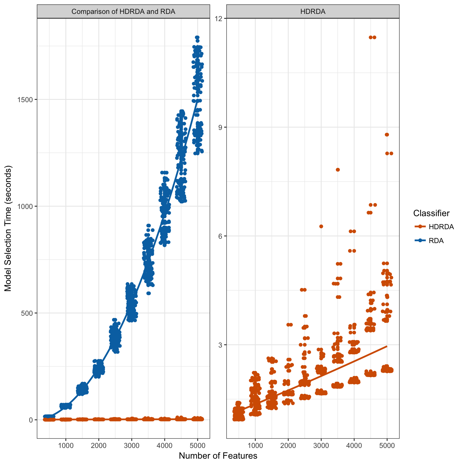
Figure 2: Timing comparisons (in seconds) between HDRDA and RDA classifiers.

In Figure 2, we plotted the runtime of the model selections for both the HDRDA and RDA classifiers as a function of $p$. We observed that the HDRDA classifier was substantially faster than the RDA classifier as $p$ increased. In the left panel of Figure 2, we fit a quadratic regression line to the RDA runtimes and a simple linear regression model to the HDRDA runtimes. For improved understanding, in the right panel we repeated the same scatterplot and linear fit with the timings restricted to the observed range of the HDRDA timings. Figure 2 suggests that the usage of a matrix inverse and determinant in the klaR R package’s discriminant function yielded model-selection timings that exceeded linear growth in $p$. Because the HDRDA classifier removes inverse and determinants, it was computationally more efficient than the RDA classifier, especially as $p$ increased. In fact, when $p=5000$, the RDA classifier required 24.933 minutes on average to perform model selection, while the HDRDA classifier selected its optimal model in 2.979 seconds on average. Clearly, the model selection employed by the HDRDA classifier is substantially faster than that of the RDA classifier.

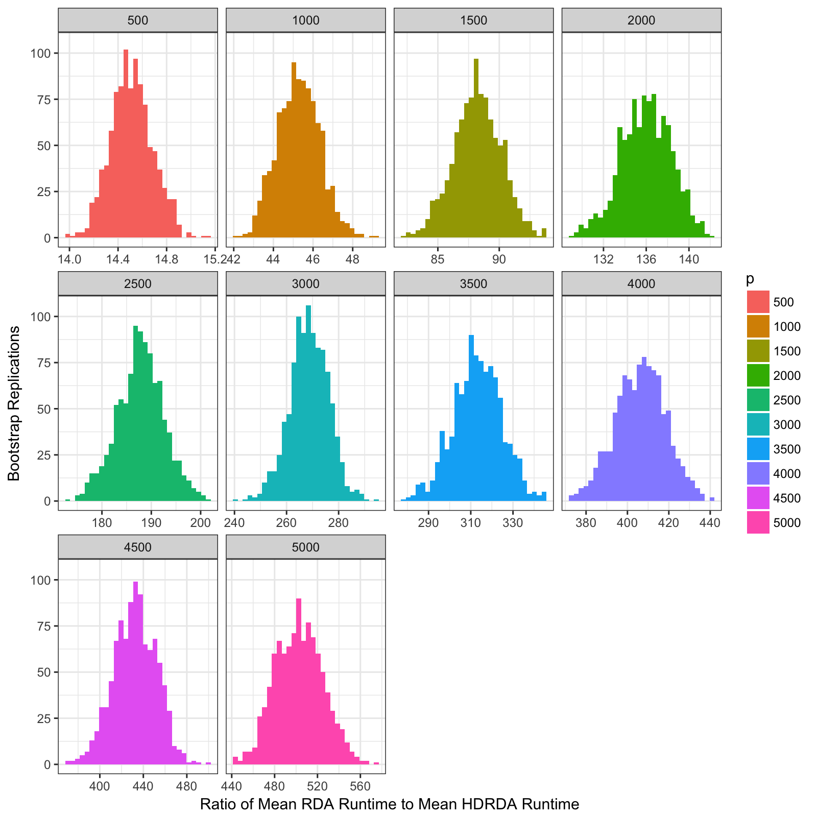
Figure 3: Distribution of ratios of mean RDA runtime to mean HDRDA runtime across 1000 bootstrap replications.

We quantified the relative timing comparisons between the two classifiers by calculating the ratio of mean timings of the RDA classifier to the HDRDA classifier for each value of $p$. We employed nonparametric bootstrapping to estimate the mean ratio along with 95% confidence intervals. In Figure 3, the bootstrap sampling distributions for the ratio of mean timings are given. First, we observe that the mean relative timings increased as $p$ increased. For smaller dimensions, the relative difference in computing was sizable with the average ratio of the mean timings equal to 14.513 for $p=500$ and a 95% confidence interval of (14.191, 14.855). Furthermore, the ratio of mean computing times suggested that the RDA classifier is impractical for higher dimensions. For instance, when $p=5000$, the ratio of mean computing times increased to 502.786 with a 95% confidence interval of (462.863, 546.396).

$$\left[\text{Insert Figure \ref{fig:timing-results} approximately here }\right]$$

$$\left[\text{Insert Figure \ref{fig:timing-comparison-bootstrap} approximately here }\right]$$

6 Classification Study

In this section, we compare our proposed classifier with four classifiers recently proposed for small-sample, high-dimensional data along with the random-forest classifier from Breiman (2001) using version 3.3.1 of the open-source statistical software R. Within our study, we included penalized linear discriminant analysis from Witten and Tibshirani (2011), implemented in the penalizedLDA package. We also considered shrunken centroids regularized discriminant analysis from Guo et al. (2007) in the rda package. Because the rda package does not perform the authors’ “Min-Min” rule automatically, we applied this rule within our R code. We included two modifications of diagonal linear discriminant analysis from Tong et al. (2012) and Pang et al. (2009), where the former employs an improved mean estimator and the latter utilizes an improved variance estimator. Both classifiers are available in the sparsediscrim package. Finally, we incorporated the random forest as a benchmark based on the findings of Fernández-Delgado et al. (2014), who concluded that the random forest is often superior to other classifiers in benchmark studies. We used the implementation of the random-forest classifier from the randomForest package with 250 trees and 100 maximum nodes. For each classifer we explicitly set prior probabilities as equal, if applicable. All other classifier options were set to their default settings. Below, we refer to each classifier by the first author’s surname. All simulations were conducted on an Amazon EC2 c4.4xlarge instance. Our analyses can be reproduced via the code available at https://github.com/ramhiser/paper-hdrda.

For the HDRDA classifier in (11), we examined the classification performance of two models. For the first HDRDA model, we set $\alpha_{k}=1$, $k=1,\ldots,K$, so that the covariance-matrix estimator (6) resembled (3). We estimated $\lambda$ from a grid of 21 equidistant candidate values between 0 and 1, inclusively. Similarly, we estimated $\gamma$ from a grid consisting of the values $10^{-1},\ldots,10^{4}$, and $10^{5}$. We selected optimal estimates of $\lambda$ and $\gamma$ using $10$-fold cross-validation. For the second model, we set $\alpha_{k}=1-\gamma$, $k=1,\ldots,K$, to resemble Friedman’s parameterization, and we estimated both $\lambda$ and $\gamma$ from a grid of 21 equidistant candidate values between 0 and 1, inclusively.

We did not include the RDA classifier in our classification study because its training runtime was prohibitively slow on high-dimensional data in our preliminary experiments. As shown in Section 5, the runtime of the RDA classifier was drastically larger than that of the HDRDA classifier for a tuning grid of size $25=5\times 5$. Consequently, a fair comparison between the RDA and HDRDA classifiers would require model selection of $441=21\times 21$ different pairs of tuning parameters in the RDA classifier. A tuning grid of this size yielded excessively slow training runtimes for the RDA implementation from the klaR R package.

6.1 Simulation Study

In this section we compare the competing classifiers using the simulation design from Guo et al. (2007). This design is widely used within the high-dimensional classification literature, including the studies by Ramey and Young (2013) and Witten and Tibshirani (2011). First, we consider the block-diagonal covariance matrix from Guo et al. (2007),

$$\bm{\Sigma}_{k}=\begin{bmatrix}\bm{\Sigma}^{(\rho_{k})}&\bm{0}_{100}&\bm{0}_{100}&\cdots&\cdots&\cdots\\ \bm{0}_{100}&\bm{\Sigma}^{(-\rho_{k})}&\bm{0}_{100}&\bm{0}_{100}&\cdots&\vdots\\ \bm{0}_{100}&\bm{0}_{100}&\bm{\Sigma}^{(\rho_{k})}&\bm{0}_{100}&\cdots&\vdots\\ \vdots&\bm{0}_{100}&\bm{0}_{100}&\bm{\Sigma}^{(-\rho_{k})}&\bm{0}_{100}&\vdots\\ \vdots&\vdots&\vdots&\bm{0}_{100}&\ddots&\vdots\\ \cdots&\cdots&\cdots&\cdots&\cdots&\cdots\\ \end{bmatrix},$$ (15)

where the $(i,j)$th entry of the block matrix $\bm{\Sigma}^{(\rho_{k})}\in\mathbb{R}_{100\times 100}$ is

$$\bm{\Sigma}_{ij}^{(\rho_{k})}=\{\rho_{k}^{|i-j|}\}_{1\leq i,j\leq 100}.$$

The block-diagonal covariance structure in (15) resembles gene-expression data: within each block of pathways, genes are correlated, and the correlation decays as a function of the distance between any two genes. The original design from Guo et al. (2007) comprised two $p$-dimensional multivariate normal populations with a common block-diagonal covariance matrix.

Although the design is indeed standard, the simulation configuration lacks artifacts commonly observed in real data, such as skewness and extreme outliers. As a result, we wished to investigate the effect of outliers on the high-dimensional classifiers. To accomplish this goal, we generalized the block-diagonal simulation configuration by sampling from a $p$-dimensional multivariate contaminated normal distribution. Denoting the PDF of the $p$-dimensional multivariate normal distribution by $N_{p}(\bm{x}|\bm{\mu},\bm{\Sigma})$, we write the PDF of the $k$th class as

$$p(\bm{x}|\omega_{k})=(1-\epsilon)N_{p}(\bm{x}|\bm{\mu}_{k},\bm{\Sigma}_{k})+\epsilon N_{p}(\bm{x}|\bm{\mu}_{k},\eta\bm{\Sigma}_{k}),$$ (16)

where $\epsilon\in[0,1]$ is the probability that an observation is contaminated (i.e., drawn from a distribution with larger variance) and $\eta>1$ scales the covariance matrix $\bm{\Sigma}_{k}$ to increase the extremity of outliers. For $\epsilon=0$, we have the benchmark block-diagonal simulation design from Guo et al. (2007). As $\epsilon$ is increased, the average number of outliers is increased. In our simulation, we let $\eta=100$ and considered the values of $\epsilon=0$, $0.05$, $\ldots$, $0.50$.

We generated $K=3$ populations from (16) with $\bm{\Sigma}_{k}$ given in (15) and set the mean vector of class 1 to $\bm{\mu}_{1}=\bm{0}_{p}$. Next, comparable to Guo et al. (2007), the first 100 features of $\bm{\mu}_{2}$ were set to 1/2, while the rest were set to 0, i.e., $\bm{\mu}_{2}=(\underbrace{1/2,\ldots,1/2}_{100},\underbrace{0,\ldots,0}_{p-100})$. For simplicity, we defined $\bm{\mu}_{3}=-\bm{\mu}_{2}$. The three populations differed in their mean vectors in the first 100 features corresponding to the first block, and no difference in the means occurred in the remaining blocks.

From each of the $K=3$ populations, we sampled 25 training observations ($n_{k}=25$ for all $k$) and 10,000 test observations. After training each classifier on the training data, we classified the test data sets and computed the proportion of mislabeled test observations to estimate the classification error rate for each classifier. Repeating this process 500 times, we computed the average of the error-rate estimates for each classifier. We allowed the number of features to vary from $p=100$ to $p=500$ in increments of 100 to examine the classification accuracy as the feature dimension increased while maintaining a small sample size. Guo et al. (2007) originally considered $\rho_{k}=0.9$ for all $k$. Alternatively, to explore the more realistic assumption of unequal covariance matrices, we put $\rho_{1}=0.1$, $\rho_{2}=0.5$, and $\rho_{3}=0.9$.

6.1.1 Simulation Results

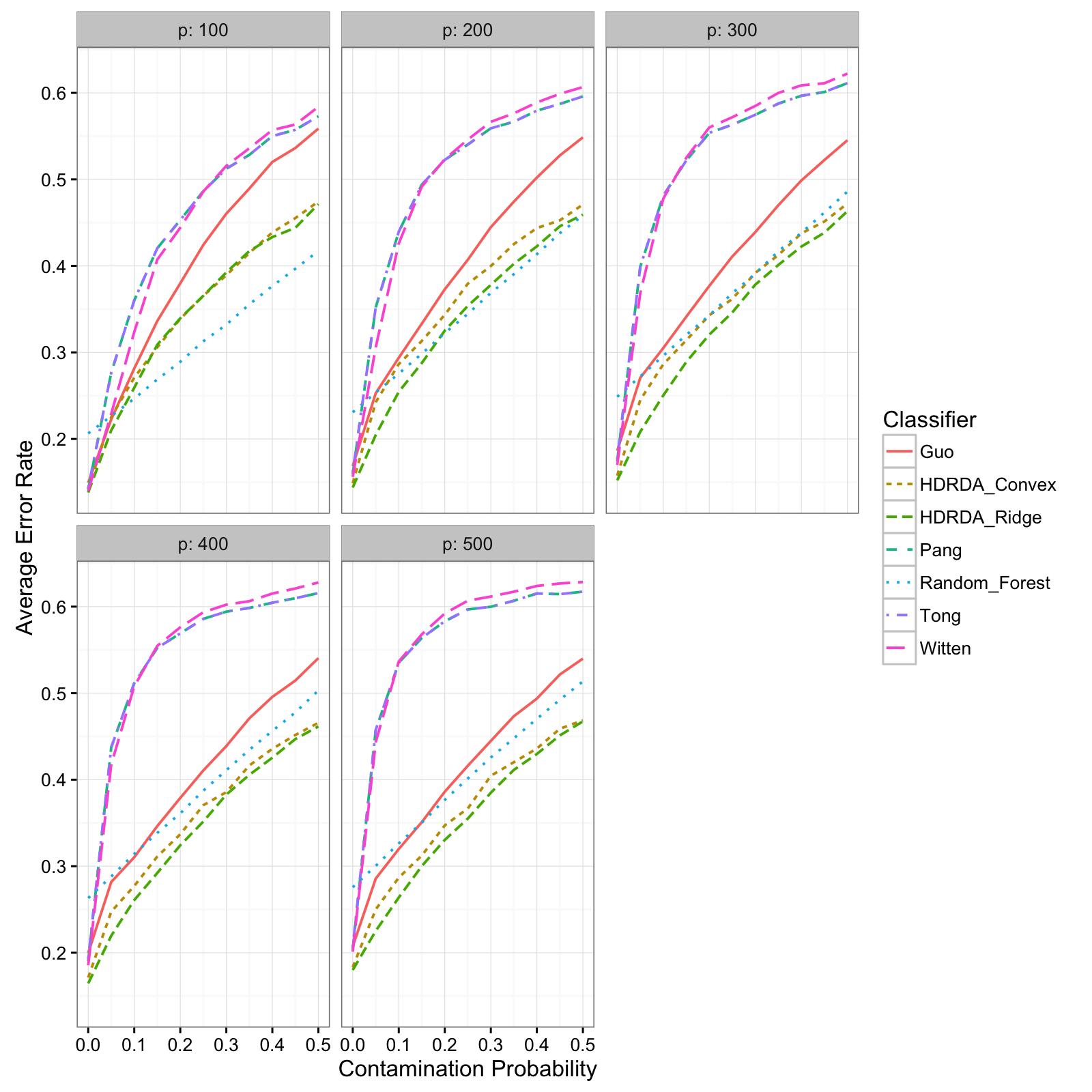
Figure 4: Average classification error rates as a function of the contamination probability $\epsilon$. Approximate standard errors were no greater than 0.022.

In Figure 4, we observed each classifier’s average classification error rates for the values of $\epsilon$ and $p$. Unsurprisingly, the average error rate increased for each classifier as the contamination probability $\epsilon$ increased regardless of the value of $p$. Sensitivity to the presence of outliers was most apparent for the Pang, Tong, and Witten classifiers. For smaller dimensions, the random-forest and HDRDA classifiers tended to outperform the remaining classifiers with the random forest performing best. As the feature dimension increased with $p\geq 300$, both HDRDA classifiers outperformed all other classifiers, suggesting that their inherent dimension reduction better captured the classificatory information in the small training samples, even in the presence of outliers.

$$\left[\text{Insert Figure \ref{fig:sim-results} approximately here }\right]$$

The Pang, Tong, and Witten methods yielded practically the same and consistently the worst error rates when outliers were present with $\epsilon>0$, suggesting that these classifiers were sensitive to outliers. Notice, for example, that when $p=400$, the error rates of the Pang, Tong, and Witten classifiers increased dramatically from approximately 19% when no outliers were present to approximately 43% when $\epsilon=0.05$. The sharp increase in average error rates for these three classifiers continued as $\epsilon$ increased. Guo’s method always outperformed those of Pang, Witten, and Tong, but after outliers were introduced, the Guo classifier’s average error rate was not competitive with the HDRDA classifiers or the random-forest classifier.

$$\left[\text{Insert Figure \ref{fig:sim-results-by-p} approximately here }\right]$$

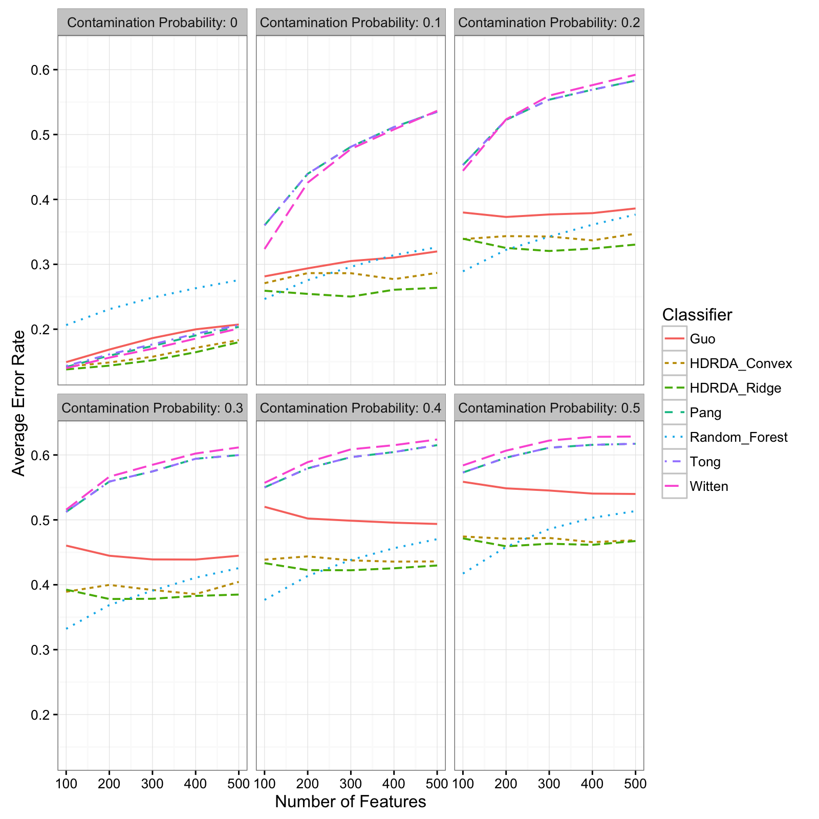
Figure 5: Average classification error rates as a function of the number of features $p$. Approximate standard errors were no greater than 0.022.

In Figure 5, we again examine the simulation results as a function of $p$ for a subset of the values of $\epsilon$. This set of plots allows us to investigate the effect of feature dimensionality on classification performance. When no outliers were present (i.e., $\epsilon=0$), the random-forest classifier was outperformed by all other classifiers. Furthermore, the HDRDA classifiers were superior in terms of average error rate in this setting. As $p$ increased, an elevation in average error rate was expected for all classifiers, but the increase was not observed to be substantial.

For $\epsilon>0$, we observed a different behavior in classification performance. First, the Pang, Tong, and Witten methods, along with the random-forest method, increased in average error rate as $p$ increased. Contrarily, the performance of the HDRDA and Guo classifiers was hardly affected by $p$. Also, as discussed above, the HDRDA classifiers were superior to all other classifiers for large values of $p$ with only the random-forest classifier outperforming them in smaller feature-dimension cases.

6.2 Application to Gene Expression Data

We compared the HDRDA classifier to the five competing classifiers on six benchmark gene-expression microarray data sets. First, we evaluated the classification accuracy of each classifier by randomly partitioning the data set under consideration such that $2/3$ of the observations were allocated as training data and the remaining $1/3$ of the observations were allocated as a test data set. To expedite the computational runtime, we reduced the training data to the top 1000 variables by employing the variable-selection method proposed by Dudoit et al. (2002). We then reduced the test data set to the same 1000 variables. After training each classifier on the training data, we classified the test data sets and computed the proportion of mislabeled test observations to estimate the classification error rate for each classifier. Repeating this process 100 times, we computed the average of the error-rate estimates for each classifier. We next provide a concise description of each high-dimensional data set examined in our classification study.

6.2.1 Chiaretti et al. (2004) Data Set

Chiaretti et al. (2004) measured the gene-expression profiles for 128 individuals with acute lymphoblastic leukemia (ALL) using Affymetrix human 95Av2 arrays. Following Xu et al. (2009), we restricted the data set to $K=2$ classes such that $n_{1}=74$ observations were without cytogenetic abnormalities and $n_{2}=37$ observations had a detected BCR/ABL gene. The robust multichip average normalization method was applied to all 12,625 gene-expression levels.

6.2.2 Chowdary et al. (2006) Data Set

Chowdary et al. (2006) investigated 52 matched pairs of tissues from colon and breast tumors using Affymetrix U133A arrays and ribonucleic-acid (RNA) amplification. Each tissue pair was gathered from the same patient and consisted of a snap-frozen tissue and a tissue suspended in an RNAlater preservative. Overall, 31 breast-cancer and 21 colon-cancer pairs were gathered, resulting in $K=2$ classes with $n_{1}=62$ and $n_{2}=42$. A purpose of the study was to determine whether the disease state could be identified using 22,283 gene-expression profiles.

6.2.3 Nakayama et al. (2007) Data Set

Nakayama et al. (2007) acquired 105 gene-expression samples of 10 types of soft-tissue tumors through an oligonucleotide microarray, including 16 samples of synovial sarcoma (SS), 19 samples of myxoid/round cell liposarcoma (MLS), 3 samples of lipoma, 3 samples of well-differentiated liposarcoma (WDLS), 15 samples of dedifferentiated liposarcoma (DDLS), 15 samples of myxofibrosarcoma (MFS), 6 samples of leiomyosarcoma (LMS), 3 samples of malignant nerve sheathe tumor (MPNST), 4 samples of fibrosarcoma (FS), and 21 samples of malignant fibrous histiocytoma (MFH). Nakayama et al. (2007) determined from their data that these 10 types fell into 4 broader groups: (1) SS; (2) MLS; (3) Lipoma, WDLS, and part of DDLS; (4) Spindle cell and pleomorophic sarcomas including DDLS, MFS, LMS, MPNST, FS, and MFH. Following Witten and Tibshirani (2011), we restricted our analysis to the five tumor types having at least 15 observations.

6.2.4 Shipp et al. (2002) Data Set

According to Shipp et al. (2002), approximately 30%-40% of adult non-Hodgkin lymphomas are diffuse large B-cell lymphomas (DLBCLs). However, only a small proportion of DLBCL patients are cured with modern chemotherapeutic regimens. Several models have been proposed, such as the International Prognostic Index (IPI), to determine a patient’s curability. These models rely on clinical covariates, such as age, to determine if the patient can be cured, and the models are often ineffective. Shipp et al. (2002) have argued that researchers need more effective means to determine a patient’s curability. The authors measured 6,817 gene-expression levels from 58 DLBCL patient samples with customized cDNA (lymphochip) microarrays to investigate the curability of patients treated with cyclophosphamide, adriamycin, vincristine, and prednisone (CHOP)-based chemotherapy. Among the 58 DLBCL patient samples, 32 are from cured patients while 26 are from patients with fatal or refractory disease.

6.2.5 Singh et al. (2002) Data Set

Singh et al. (2002) have examined 235 radical prostatectomy specimens from surgery patients between 1995 and 1997. The authors used oligonucleotide microarrays containing probes for approximately 12,600 genes and expressed sequence tags. They have reported that 102 of the radical prostatectomy specimens are of high quality: 52 prostate tumor samples and 50 non-tumor prostate samples.

6.2.6 Tian et al. (2003) Data Set

Tian et al. (2003) investigated the purified plasma cells from the bone marrow of control patients along with patients with newly diagnosed multiple myeloma. Expression profiles for 12,2625 genes were obtained via Affymetrix U95Av2 microarrays. The plasma cells were subjected to biochemical and immunohistochemical analyses to identify molecular determinants of osteolytic lesions. For 36 multiple-myloma patients, focal bone lesions could not be detected by magnetic resonance imaging (MRI), whereas MRI was used to detect such lesions in 137 patients.

6.2.7 Classification Results

Similar to Witten and Tibshirani (2011), we report the average test error rates obtained over 100 random training-test partitions in Table 1 along with standard deviations of the test error rates in parentheses. The HDRDA and Guo classifiers were superior in classification performance for the majority of the simulations. The HDRDA classifiers yielded the best classification accuracy on the Chowdary and Shipp data sets. Although the random forest’s accuracy slightly exceeded the HDRDA classifiers on the Tian data set, our proposed classifiers outperformed the other competing classifiers considered here. Moreover, the HDRDA classifiers yielded comparable performance on five of the six data sets.

$$\left[\text{Insert Table \ref{tab:microarray-results} approximately here }\right]$$

The average error-rate estimates for the Pang, Tong, and Witten classifiers were comparable across all six data sets. Furthermore, the average error rates for the Pang and Tong classifiers were approximately equal for all data sets except for the Chiaretti dataset. This result suggests that the mean and variance estimators used in lieu of the MLEs provided little improvement to classification accuracies. However, we investigated the Pang classifier’s poor performance on the Chiaretti data set and determined that its variance estimator exhibited numerical instability. The classifier’s denominator was approximately zero for both classes and led to the poor classification performance.

The random-forest classifier was competitive when applied to the Chowdary and Singh data sets and yielded the smallest error rate of the considered classifiers on the Tian data set. The fact that the HDRDA and Guo classifiers typically outperformed the random-forest classifier challenges the claim of Fernández-Delgado et al. (2014) that random forests are typically superior. Further studies should be performed to validate this statement in the small-sample, high-dimensional setting.

Finally, the Pang, Tong, and Witten classifiers consistently yielded the largest average error rates across the six data sets. Given that the standard deviations were relatively large, we hesitate to generalize claims regarding the ranking of these three classifiers in terms of the average error rate. However, the classifiers’ error rates and their variability across multiple random partitions of each data set were large enough that we might question their benefit when applied to real data.

7 Discussion

We have demonstrated that our proposed HDRDA classifier is competitive with and often superior to random forests as well as the Witten, Pang, Tong, and Guo classifiers. In fact, we have shown that the HDRDA classifier often yields superior classification accuracy when applied to small-sample, high-dimensional data sets, confirming the assertions of Mai et al. (2012) and Fan et al. (2012) that diagonal classifiers often yield inferior classification performance when compared to other classification methods. Furthermore, we have demonstrated that HDRDA classifiers are more robust to the presence of outliers than the diagonal classifiers despite their rapid computational performance and their reduction in the number of parameters to estimate.

We also considered the popular penalized linear discriminant analysis from Witten and Tibshirani (2011) because it was specifically designed for high-dimensional gene-expression data. We had expected its classification performance to be competitive within our classification study and perhaps superior. Contrarily, our empirical studies suggest that the classifier is sensitive to outliers and unable to achieve comparable results with other classifiers designed for small-sample, high-dimensional data. Also, despite the claims of Fernández-Delgado et al. (2014) that random forests are typically superior to other classifiers, we observed that they were indeed competitive but were typically outperformed by classifiers developed for small-sample, high-dimensional data.

We demonstrated that our HDRDA implementation in the sparsediscrim R package can be used in practice with high-dimensional data sets. In our timing comparisons, we showed that HDRDA model selection could be employed on data sets with $p=5000$ in 2.979 seconds on average. Contrarily, the RDA classifier implemented in the klaR R package required 24.933 minutes on average to perform model selection on data sets with $p=5000$. Given that the RDA classifier has been shown to have excellent performance in the high-dimensional setting (Webb and Copsey, 2011) but is limited by its computationally intense model-selection procedure, our work replaces the RDA classifier for high-dimensional data in practice. This result is reassuring because the RDA classifier remains widely popular in the literature. In fact, variants of the RDA classifier have been applied to microarray data (Ching et al., 2012; Li and Wu, 2012; Tai and Pan, 2007; Guo et al., 2007), facial recognition (Zhang et al., 2010; Dai and Yuen, 2007; Lu et al., 2005; Pima and Aladjem, 2004; Lu and Plataniotis, 2003), handwritten digit recognition (Bouveyron et al., 2007), remote sensing (Tadjudin and Landgrebe, 1999), seismic detection (Anderson, 2002), and chemical spectra (Wu et al., 1996; Aeberhard et al., 1993).

The dimension reduction employed in this paper has reduced the dimension to rank$(\widehat{\bm{\Sigma}})=q$. An interesting extension of our work would reduce the dimension $q$ further to a lower dimension $q_{L}<q$, perhaps using a criterion similar to that of principal components analysis. While unclear whether the classification performance would improve via such a method, the efficiency of the model selection would certainly improve. Moreover, if $q_{L}=2$ or $3$, low-dimensional graphical displays of high-dimensional data could be obtained.

We thank Mrs. Joy Young for her numerous recommendations that enhanced the quality of our writing.

Classifier	Chiaretti	Chowdary	Nakayama	Shipp	Singh	Tian
Guo	0.111 (0.044)	0.056 (0.051)	0.208 (0.061)	0.086 (0.063)	0.089 (0.055)	0.268 (0.082)
HDRDA Convex	0.115 (0.044)	0.035 (0.026)	0.208 (0.066)	0.073 (0.057)	0.111 (0.059)	0.229 (0.049)
HDRDA Ridge	0.118 (0.050)	0.033 (0.022)	0.208 (0.070)	0.072 (0.065)	0.099 (0.046)	0.225 (0.050)
Pang	0.663 (0.062)	0.197 (0.091)	0.227 (0.062)	0.192 (0.091)	0.221 (0.095)	0.267 (0.054)
Random Forest	0.124 (0.053)	0.045 (0.028)	0.232 (0.063)	0.135 (0.078)	0.093 (0.045)	0.206 (0.044)
Tong	0.195 (0.068)	0.197 (0.091)	0.227 (0.062)	0.192 (0.091)	0.221 (0.095)	0.267 (0.054)
Witten	0.194 (0.068)	0.197 (0.091)	0.232 (0.068)	0.193 (0.092)	0.221 (0.095)	0.264 (0.053)

Table 1: The average of the test error rates obtained on gene-expression data sets over 100 random training-test partitions. Standard deviations of the test error rates are given in the parentheses. The classifier with the minimum average error rate for each data set is in bold.

References

- Aeberhard et al. (1993) Aeberhard, S., Coomans, D., Vel, O. D., 1993. Improvements to the classification performance of RDA. Journal of Chemometrics 7 (2), 99–115.
- Anderson (2002) Anderson, D. N., Aug. 2002. Application of Regularized Discrimination Analysis to Regional Seismic Event Identification. Bulletin of the Seismological Society of America 92 (6), 2391–2399.
- Bensmail and Celeux (1996) Bensmail, H., Celeux, G., Dec. 1996. Regularized Gaussian Discriminant Analysis through Eigenvalue Decomposition. Journal of the American Statistical Association 91 (436), 1743–1748.
- Bouveyron et al. (2007) Bouveyron, C., Girard, S., Schmid, C., Oct. 2007. High-Dimensional Discriminant Analysis. Communications in Statistics - Theory and Methods 36 (14), 2607–2623.
- Breiman (2001) Breiman, L., 2001. Random Forests - Springer. Machine Learning 45 (1), 5–32.
- Chiaretti et al. (2004) Chiaretti, S., Li, X., Gentleman, R., Vitale, A., Vignetti, M., Mandelli, F., Ritz, J., Foa, R., 2004. Gene expression profile of adult T-cell acute lymphocytic leukemia identifies distinct subsets of patients with different response to therapy and survival. Blood 103 (7), 2771–2778.
- Ching et al. (2012) Ching, W.-K., Chu, D., Liao, L.-Z., Wang, X., Jul. 2012. Regularized orthogonal linear discriminant analysis. Pattern Recognition 45 (7), 2719–2732.
- Chowdary et al. (2006) Chowdary, D., Lathrop, J., Skelton, J., Curtin, K., Briggs, T., Zhang, Y., Yu, J., Wang, Y., Mazumder, A., Feb. 2006. Prognostic Gene Expression Signatures Can Be Measured in Tissues Collected in RNAlater Preservative. The Journal of Molecular Diagnostics 8 (1), 31–39.
- Dai and Yuen (2007) Dai, D.-Q., Yuen, P. C., Aug. 2007. Face recognition by regularized discriminant analysis. IEEE transactions on systems, man, and cybernetics. Part B, Cybernetics : a publication of the IEEE Systems, Man, and Cybernetics Society 37 (4), 1080–1085.
- Dudoit et al. (2002) Dudoit, S., Fridlyand, J., Speed, T. P., Mar. 2002. Comparison of Discrimination Methods for the Classification of Tumors Using Gene Expression Data. Journal of the American Statistical Association 97 (457), 77–87.
- Fan et al. (2012) Fan, J., Feng, Y., Tong, X., Apr. 2012. A road to classification in high dimensional space: the regularized optimal affine discriminant. Journal of the Royal Statistical Society: Series B (Statistical Methodology) 74 (4), 745–771.
- Fernández-Delgado et al. (2014) Fernández-Delgado, M., Cernadas, E., Barro, S., Amorim, D., Jan. 2014. Do we need hundreds of classifiers to solve real world classification problems? The Journal of Machine Learning Research 15 (1), 3133–3181.
- Friedman (1989) Friedman, J. H., 1989. Regularized Discriminant Analysis. Journal of the American Statistical Association 84 (405), 165–175.
- Guo et al. (2007) Guo, Y., Hastie, T., Tibshirani, R., Jan. 2007. Regularized linear discriminant analysis and its application in microarrays. Biostatistics 8 (1), 86–100.
- Halbe and Aladjem (2007) Halbe, Z., Aladjem, M., Nov. 2007. Regularized mixture discriminant analysis. Pattern Recognition Letters 28 (15), 2104–2115.
- Harville (2008) Harville, D. A., 2008. Matrix Algebra from a Statistician’s Perspective. Springer, New York.
- Hastie et al. (2008) Hastie, T., Tibshirani, R., Friedman, J., Dec. 2008. The Elements of Statistical Learning, 2nd Edition. Data Mining, Inference, and Prediction. Springer New York, New York, NY.
- Hoerl and Kennard (1970) Hoerl, A. E., Kennard, R. W., Feb. 1970. Ridge Regression: Biased Estimation for Nonorthogonal Problems. Technometrics 12 (1), 55–67.
- Kollo and von Rosen (2005) Kollo, T., von Rosen, D., 2005. Advanced Multivariate Statistics with Matrices. Vol. 579 of Mathematics and Its Applications (New York). Springer, Dordrecht.
- Li and Wu (2012) Li, R., Wu, B., Aug. 2012. Sparse regularized discriminant analysis with application to microarrays. Computational biology and chemistry 39, 14–19.
- Lu and Plataniotis (2003) Lu, J., Plataniotis, K. N., 2003. Regularized discriminant analysis for the small sample size problem in face recognition. Pattern Recognition Letters.
- Lu et al. (2005) Lu, J., Plataniotis, K. N., Venetsanopoulos, A. N., 2005. Regularization studies of linear discriminant analysis in small sample size scenarios with application to face recognition. Pattern Recognition Letters 26 (2), 181–191.
- Mai et al. (2012) Mai, Q., Zou, H., Yuan, M., Feb. 2012. A direct approach to sparse discriminant analysis in ultra-high dimensions. Biometrika 99 (1), 29–42.
- Mkhadri (1995) Mkhadri, A., Mar. 1995. Shrinkage parameter for the modified linear discriminant analysis. Pattern Recognition Letters 16 (3), 267–275.
- Mkhadri et al. (1997) Mkhadri, A., Celeux, G., Nasroallah, A., 1997. Regularization in discriminant analysis: an overview. Computational Statistics and Data Analysis 23 (3), 403–423.
- Murphy (2012) Murphy, K. P., Aug. 2012. Machine Learning: A Probabilistic Perspective. The MIT Press, Cambridge, Massachusetts.
- Nakayama et al. (2007) Nakayama, R., Nemoto, T., Takahashi, H., Ohta, T., Kawai, A., Seki, K., Yoshida, T., Toyama, Y., Ichikawa, H., Hasegawa, T., Apr. 2007. Gene expression analysis of soft tissue sarcomas: characterization and reclassification of malignant fibrous histiocytoma. Nature 20 (7), 749–759.
- Pang et al. (2009) Pang, H., Tong, T., Zhao, H., Mar. 2009. Shrinkage-based Diagonal Discriminant Analysis and Its Applications in High-Dimensional Data. Biometrics 65 (4), 1021–1029.
- Pima and Aladjem (2004) Pima, I., Aladjem, M., 2004. Regularized discriminant analysis for face recognition. Pattern Recognition 37 (9), 1945–1948.
- Ramey and Young (2013) Ramey, J., Young, P. D., 2013. A comparison of regularization methods applied to the linear discriminant function with high-dimensional microarray data. Journal of Statistical Computation and Simulation 83 (3), 581–596.
- Rao and Mitra (1971) Rao, C. R., Mitra, S. K., 1971. Generalized inverse of a matrix and its applications. In: Proceedings of the Sixth Berkeley Symposium on Mathematical Statistics and Probability. University of California Press, Berkeley, pp. 601–620.
- Seber (2004) Seber, G. A. F., Aug. 2004. Multivariate Observations. Wiley Series in Probability and Statistics. Wiley-Interscience.
- Shipp et al. (2002) Shipp, M. A., Ross, K. N., Tamayo, P., Weng, A. P., Kutok, J. L., Aguiar, R. C. T., Gaasenbeek, M., Angelo, M., Reich, M., Pinkus, G. S., Ray, T. S., Koval, M. A., Last, K. W., Norton, A., Lister, T. A., Mesirov, J., Neuberg, D. S., Lander, E. S., Aster, J. C., Golub, T. R., Jan. 2002. Diffuse large B-cell lymphoma outcome prediction by gene-expression profiling and supervised machine learning. Nature Medicine 8 (1), 68–74.
- Singh et al. (2002) Singh, D., Febbo, P. G., Ross, K., Jackson, D. G., Manola, J., Ladd, C., Tamayo, P., Renshaw, A. A., D’Amico, A. V., Richie, J. P., Lander, E. S., Loda, M., Kantoff, P. W., Golub, T. R., Sellers, W. R., Mar. 2002. Gene expression correlates of clinical prostate cancer behavior. Cancer Cell 1 (2), 203–209.
- Srivastava and Kubokawa (2007) Srivastava, M. S., Kubokawa, T., 2007. Comparison of discrimination methods for high dimensional data. Journal of the Japan Statistical Society 37 (1), 123–134.
- Tadjudin and Landgrebe (1999) Tadjudin, S., Landgrebe, D. A., Jul. 1999. Covariance estimation with limited training samples. IEEE Transactions on Geoscience and Remote Sensing 37 (4), 2113–2118.
- Tai and Pan (2007) Tai, F., Pan, W., Dec. 2007. Incorporating prior knowledge of gene functional groups into regularized discriminant analysis of microarray data. Bioinformatics 23 (23), 3170–3177.
- Tian et al. (2003) Tian, E., Zhan, F., Walker, R., Rasmussen, E., Ma, Y., Barlogie, B., Shaughnessy, Jr., J. D., Dec. 2003. The Role of the Wnt-Signaling Antagonist DKK1 in the Development of Osteolytic Lesions in Multiple Myeloma. New England Journal of Medicine 349 (26), 2483–2494.
- Tong et al. (2012) Tong, T., Chen, L., Zhao, H., Feb. 2012. Improved mean estimation and its application to diagonal discriminant analysis. Bioinformatics 28 (4), 531–537.
- Webb and Copsey (2011) Webb, A. R., Copsey, K. D., Sep. 2011. Statistical Pattern Recognition, 3rd Edition. John Wiley & Sons, Chichester, West Sussex, UK.
- Witten and Tibshirani (2011) Witten, D. M., Tibshirani, R., Aug. 2011. Penalized classification using Fisher’s linear discriminant. Journal of the Royal Statistical Society: Series B (Statistical Methodology) 73 (5), 753–772.
- Wu et al. (1996) Wu, W., Mallet, Y., Walczak, B., Penninckx, W., Massart, D. L., Heuerding, S., Erni, F., Aug. 1996. Comparison of regularized discriminant analysis, linear discriminant analysis, and quadratic discriminant analysis applied to NIR data. Analytica Chimica Acta 329 (3), 257–265.
- Xu et al. (2009) Xu, P., Brock, G. N., Parrish, R. S., Mar. 2009. Modified linear discriminant analysis approaches for classification of high-dimensional microarray data. Computational Statistics and Data Analysis 53 (5), 1674–1687.
- Ye and Ji (2009) Ye, J., Ji, S., Nov. 2009. Discriminant Analysis for Dimensionality Reduction: An Overview of Recent Developments. Biometrics: Theory, Methods, and Applications. John Wiley & Sons, Inc., Hoboken, NJ, USA.
- Ye and Wang (2006) Ye, J., Wang, T., 2006. Regularized Discriminant Analysis for High Dimensional, Low Sample Size Data. In: The 12th ACM SIGKDD International Conference. ACM Press, New York, New York, USA, p. 454.
- Zhang et al. (2010) Zhang, Z., Dai, G., Xu, C., Jordan, M. I., Mar. 2010. Regularized Discriminant Analysis, Ridge Regression and Beyond. The Journal of Machine Learning Research 11.