The SLUGGS Survey: globular clusters and the dark matter content of early-type galaxies

Duncan A. Forbes¹, Adebusola Alabi¹, Aaron J. Romanowsky^2,3, Jean P. Brodie³, Jay Strader⁴ Christopher Usher⁵, Vincenzo Pota⁶
¹Centre for Astrophysics & Supercomputing, Swinburne University, Hawthorn VIC 3122, Australia
²Department of Physics and Astronomy, San José State University, One Washington Square, San Jose, CA 95192, USA
³University of California Observatories, 1156 High Street, Santa Cruz, CA 95064, USA
⁴Department of Physics and Astronomy, Michigan State University, East Lansing, Michigan 48824, USA
⁵Astrophysics Research Institute, Liverpool John Moores University, 146 Brownlow Hill, Liverpool L3 5RF, UK
⁶INAF - Osservatorio Astronomico di Capodimonte, Salita Moiariello, 16, 80131 Napoli, Italy E-mail: dforbes@swin.edu.au

Abstract

A strong correlation exists between the total mass of a globular cluster (GC) system and the virial halo mass of the host galaxy. However, the total halo mass in this correlation is a statistical measure conducted on spatial scales that are some ten times that of a typical GC system. Here we investigate the connection between GC systems and galaxy’s dark matter on comparable spatial scales, using dynamical masses measured on a galaxy-by-galaxy basis. Our sample consists of 17 well-studied massive (stellar mass $\sim$ 10¹¹ M_⊙) early-type galaxies from the SLUGGS survey. We find the strongest correlation to be that of the blue (metal-poor) GC subpopulation and the dark matter content. This correlation implies that the dark matter mass of a galaxy can be estimated to within a factor of two from careful imaging of its GC system. The ratio of the GC system mass to that of the enclosed dark matter is nearly constant. We also find a strong correlation between the fraction of blue GCs and the fraction of enclosed dark matter, so that a typical galaxy with a blue GC fraction of 60 per cent has a dark matter fraction of 86 per cent over similar spatial scales. Both halo growth and removal (via tidal stripping) may play some role in shaping this trend. In the context of the two-phase model for galaxy formation, we find galaxies with the highest fractions of accreted stars to have higher dark matter fractions for a given fraction of blue GCs.

keywords:

galaxies: star clusters – galaxies: evolution

^†^†pagerange: The SLUGGS Survey: globular clusters and the dark matter content of early-type galaxies–LABEL:lastpage^†^†pubyear: 2002

1 Introduction

The globular cluster (GC) systems of galaxies, including the Milky Way and M31, reveal a remarkable correlation with galaxy halo mass. The correlation has a slope consistent with unity so that the ratio of the total GC system mass (M_GCS) to the total halo mass (M_h) is roughly constant with a value of a few times 10^-5 over 5 orders of magnitude (Blakeslee et al. 1997; Spitler et al. 2008; Spitler & Forbes 2009; Georgiev et al. 2010; Harris et al. 2013; Hudson et al. 2014; Durrell et al. 2014; Harris et al. 2015). The scatter of the correlation is about 0.3 dex (e.g. Harris et al. 2015).

This near linear relation may simply reflect the gas content of a given dark matter halo at the time of GC formation and is close to the scaling predicted by Kravtsov & Gnedin (2005) of M ${}_{GCS}\propto M_{h}^{1.13\pm 0.08}$ from their cosmological simulation. Over cosmic time, it is expected that the ratio M_GCS/M_h is reduced due to GC destruction (Katz & Ricotti 2014). For further discussion of these issues we refer the reader to Harris et al. (2015).

The GC systems of large galaxies also reveal a bimodal colour distribution that is well represented by blue and red subpopulations. This bimodality is in turn thought to reflect differences in metallicity (Brodie et al. 2012; Usher et al. 2012). Based on spatial distributions, metallicities and kinematics, previous GC studies have generally associated the red/metal-rich subpopulation with the stellar bulge/elliptical component of galaxies, and the blue/metal-poor subpopulation with the halo (Forte et al. 2007; Forbes et al. 2012; Pota et al. 2013; Forte et al. 2014). In the currently popular two-phase scenario for early-type galaxy formation (e.g. Oser et al. 2010), the halo is largely built up by stars formed ‘ex-situ’ in lower mass satellites which are later accreted. However, as well as an accretion origin, GC system metallicity gradients observed in a few well studied galaxies suggest that some blue GCs may have formed ‘in-situ’ along with the bulk of the red GCs (Harris 2009; Forbes et al. 2011).

It is thus important to investigate which GC subpopulation (i.e. blue or red) correlates with the dark matter content of a galaxy. In the largest study to date, Harris et al. (2015) split some 300 GC systems into blue and red subpopulations, and examined the correlation with halo mass (derived from a weak lensing study and a statistical relationship between stellar and halo mass). They found the blue GCs to have a slope close to unity, with the red GCs revealing a significantly steeper slope. Both subpopulations revealed similar scatter.

One limitation of past work is that GC systems, which have a radial extent of about ten R_e (the half-light radius of the galaxy starlight), have been compared to halo masses which are measured on scales of the virial radius or $\sim$ 100 R_e. It is unclear whether the relation holds for spatial scales that are better matched (although see Kavelaars 1999 for an early investigation), and in particular if the red/blue GC fractions vary with the enclosed dark matter fraction or the enclosed dark matter mass.

Such a connection between GCs and dark matter on comparable scales is plausible because GCs are very old (e.g. Forbes et al. 2015) and formed during the early phases of collapse of their host dark matter halos. The GCs should therefore be preferentially associated with the central regions of present-day dark matter halos (Diemand et al. 2005), rather than with the total halo mass, whose late-time growth may be dominated more by “pseudo-evolution” than by true infall (Diemer et al. 2013).

Here we use recent dynamical estimates of the dark matter content of individual early-type galaxies at radii comparable to their GC systems. In particular, we examine the dark matter on both a fixed spatial scale of 8 R_e and on a scale that matches the maximum extent of each GC system. Our sample consists of massive early-type galaxies with high quality GC system imaging and estimates of their enclosed dark matter content. Also for the first time, we use dynamical estimates of the dark matter mass rather than statistical scaling relations in the comparison with GC system mass.

2 Data

The galaxy sample for this work comes from the SLUGGS survey (http://sluggs.swin.edu.au) of nearby early-type galaxies (Brodie et al. 2014). The survey focuses on both the galaxy starlight and the GC systems of the galaxies. The galaxies cover a range of environments from the field to central dominant cluster galaxies. All have stellar masses greater than 10.3 in the log, and so probe the high mass end of the U-shaped number of GCs per unit stellar mass relation (Forbes 2005; Peng et al. 2008).

We take total (i.e. the pressure-supported mass plus the rotation mass) galaxy mass estimates from the recent work of Alabi et al. (2016) who applied the tracer mass estimator (TME) eq. 26 of Watkins et al. (2010) to some 3500 GC radial velocities under the assumption of isotropic orbits. These velocities were obtained mostly with the Keck telescope and the DEIMOS multi-object spectrograph. The TME gives galaxy mass estimates that are within a factor of two compared to those published using X-ray gas, Planetary Nebulae (PNe), and stellar kinematics for the same galaxies at the equivalent radius. Here we include mass estimates from Alabi et al. for the 16 SLUGGS and 1 bonus galaxy for which the GC data all reach at least 8 R_e. The mass of each GC system is based on the number of GCs which is sourced mainly from the imaging compilation of Harris et al. (2013) supplemented by some more recent wide-field imaging studies (Blom et al. 2012; Usher et al. 2013, Kartha et al. 2014, 2015). The sample and data used in this work are summarised in Table 1.

Table 1: Galaxy sample and properties

Galaxy	Dist.	R_e	Env.	log M_∗	GCS	$f_{\rm blue}$	$N_{\rm GC}$	f_DM (8R_e)	M_DM (8R_e)	R_max	f_DM (R_max)	M_DM (R_max)
$\rm[NGC]$	[Mpc]	[kpc]		[ $\rm M_{\odot}$ ]	[kpc]				[ $10^{11}\rm M_{\odot}$ ]	[R_e]		[ $10^{11}\rm M_{\odot}$ ]
(1)	(2)	(3)	(4)	(5)	(6)	(7)	(8)	(9)	(10)	(11)	(12)	(13)
720	26.9	4.56	F	11.35	78	0.64 $\pm$ 0.05	1489 $\pm$ 96	0.65 $\pm$ 0.09	3.88 $\pm$ 1.22	19.1	0.81 $\pm$ 0.05	9.60 $\pm$ 2.02
821	23.4	4.54	F	10.97	26	0.70 $\pm$ 0.05	320 $\pm$ 45	0.85 $\pm$ 0.04	4.90 $\pm$ 0.97	8.7	0.85 $\pm$ 0.04	4.92 $\pm$ 1.00
1023	11.1	2.58	G	10.98	20	0.43 $\pm$ 0.05	548 $\pm$ 59	0.63 $\pm$ 0.08	1.52 $\pm$ 0.32	16.2	0.76 $\pm$ 0.05	2.99 $\pm$ 0.52
1407	26.8	8.19	G	11.60	162	0.60 $\pm$ 0.05	7000 $\pm$ 2000	0.82 $\pm$ 0.04	16.36 $\pm$ 1.66	14.1	0.89 $\pm$ 0.02	32.76 $\pm$ 2.69
2768	21.8	6.66	G	11.28	63	0.65 $\pm$ 0.05	744 $\pm$ 68	0.83 $\pm$ 0.05	8.75 $\pm$ 1.38	11.4	0.83 $\pm$ 0.05	9.05 $\pm$ 1.45
3115	9.4	1.59	F	10.97	22^†	0.52 $\pm$ 0.04	550 $\pm$ 80	0.56 $\pm$ 0.07	1.17 $\pm$ 0.25	18.4	0.77 $\pm$ 0.03	3.09 $\pm$ 0.42
3377	10.9	1.90	G	10.44	27^†	0.48 $\pm$ 0.05	191 $\pm$ 15	0.69 $\pm$ 0.06	0.59 $\pm$ 0.12	14.3	0.78 $\pm$ 0.04	0.97 $\pm$ 0.16
3608	22.3	3.24	G	10.82	43	0.65 $\pm$ 0.06	450 $\pm$ 200	0.83 $\pm$ 0.09	3.08 $\pm$ 1.03	9.8	0.85 $\pm$ 0.09	3.56 $\pm$ 1.18
4278	15.6	2.42	G	10.88	64	0.66 $\pm$ 0.03	1378 $\pm$ 194	0.83 $\pm$ 0.04	3.62 $\pm$ 0.43	14.9	0.89 $\pm$ 0.03	5.87 $\pm$ 0.59
4365	23.1	5.94	G	11.48	133	0.43 $\pm$ 0.01	6450 $\pm$ 110	0.84 $\pm$ 0.03	14.37 $\pm$ 1.65	12.9	0.90 $\pm$ 0.02	25.27 $\pm$ 2.56
4374	18.5	4.75	C	11.46	30	0.89 $\pm$ 0.05	4301 $\pm$ 1201	0.89 $\pm$ 0.04	20.72 $\pm$ 5.31	9.2	0.89 $\pm$ 0.03	22.82 $\pm$ 5.50
4473	15.2	1.99	C	10.87	28^†	0.57 $\pm$ 0.05	376 $\pm$ 97	0.64 $\pm$ 0.08	1.29 $\pm$ 0.34	17.4	0.79 $\pm$ 0.04	2.77 $\pm$ 0.47
4486	16.7	6.56	C	11.53	92^†	0.73 $\pm$ 0.05	13000 $\pm$ 800	0.90 $\pm$ 0.01	29.53 $\pm$ 2.16	30.5	0.97 $\pm$ 0.01	112.83 $\pm$ 6.43
4494	16.6	3.94	G	11.02	55^†	0.72 $\pm$ 0.04	392 $\pm$ 49	0.34 $\pm$ 0.13	0.50 $\pm$ 0.21	8.5	0.36 $\pm$ 0.12	0.56 $\pm$ 0.21
4526	16.4	3.58	C	11.23	50^†	0.62 $\pm$ 0.10	388 $\pm$ 117	0.54 $\pm$ 0.15	1.89 $\pm$ 0.41	12.1	0.58 $\pm$ 0.10	2.35 $\pm$ 0.56
4649	16.5	5.28	C	11.55	40	0.63 $\pm$ 0.05	4000 $\pm$ 500	0.79 $\pm$ 0.04	12.75 $\pm$ 1.11	24.3	0.93 $\pm$ 0.01	46.24 $\pm$ 3.53
3607	22.2	4.20	G	11.29	61	0.45 $\pm$ 0.06	600 $\pm$ 200	0.66 $\pm$ 0.18	3.64 $\pm$ 1.41	20.7	0.81 $\pm$ 0.08	8.35 $\pm$ 2.45

Notes: columns are (1) galaxy name, (2) distance, (3) effective radius and (4) environment (Field, Group or Cluster) from Brodie et al. (2014), (5) log total stellar mass from Forbes et al. (2015) with an assumed error of $\pm$ 0.2 dex (to allow for reasonable variations in IMF, age and metallicity), (6) globular cluster system extent from Kartha et al. (2015) or ${\dagger}$ assumed to be 14 $\times$ the galaxy effective radius, (7) fraction of blue globular clusters and (8) total number of globular clusters from the compilation of Harris et al. (2013), except where we have used more recent wide-field imaging studies, i.e. NGC 720, 1023 and 2768 (Kartha et al. 2014), NGC 4278 (Usher et al. 2013), NGC 4365 (Blom et al. 2012), and for the blue GC fractions for NGC 3607 and NGC 3608 we use Kartha et al. (2015). We also note that there was a typo in Foster et al. (2011) so the blue and red GC numbers were swapped by mistake. Additional columns are (9) dark matter fraction and (10) dark matter mass within 8 R_e, (11) maximum radius of the GC system in galaxy effective radii, (12) dark matter fraction and (13) dark matter mass within R_max from Alabi et al. (2015). NGC 3607 is a SLUGGS bonus galaxy.

3 Results and Discussion

The extent of a GC system scales with the mass and size of the host galaxy. In particular, they typically extend to about 14 $\times$ the galaxy effective radius (Kartha et al. 2015). Previously, GC system numbers, or inferred total GC system masses, have been compared to virial masses which are measured on scales of $\sim$ 100 R_e. Here, we first probe the galaxy dark matter within a fixed 8 R_e, then second, we probe the galaxy dark matter at the maximum radius for which GC velocities and mass estimates are available. The latter naturally probes each individual GC system on a spatial scale that is closely matched to the imaging (from which GC mass estimates are derived).

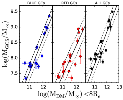
Refer to caption — Figure 1: Globular cluster system mass versus dark matter mass within 8 R_e. The total mass contained in the blue, red and all GCs is calculated assuming a constant mean GC mass. Solid and dashed lines show the best fit and 1 $\sigma$ scatter. The blue, red and all GCs correlate with the enclosed dark matter content, with the blue subpopulation having the tightest relation.

To calculate the total mass in each GC subpopulation, we start with an estimate of the total number of GCs and assign the appropriate fraction to each subpopulation based on the literature studies (see Table 1). We then use a mean GC mass of $2.4\times 10^{5}~{}\rm M_{\odot}$ as used by Spitler et al. (2008) and Durrell et al. (2014) to estimate the mass in each GC subpopulation. Variations of the mean mass with subpopulation will only change the normalisation of Fig. 1. Similarly, variations of the mean mass with galaxy magnitude are not included due to the small magnitude range of our sample.

The dark matter mass (M_DM) within 8 R_e (as listed in Table 1) is calculated from the total mass (M_tot) minus the stellar mass (M_∗) within 8 R_e (see Alabi et al. 2016 for details). We note that the dark matter mass contained within 8 R_e is $\sim$ 10 per cent of the total virial dark matter mass for a massive halo with an NFW-like profile.

Fig. 1 shows that the mass of the blue, red and all GCs have a strong correlation with the dark matter content within 8 R_e. A similar finding was found by Harris et al. (2015) who used the total halo virial mass. Our results from a linear fit to the data are given in Table 2. Here we use a generalised chi-squared minimisation fit as given in the R package called hyper.fit. A weighted fit is performed on both coordinates based on their uncertainities, with an assumption that their uncertainties are independent. All data points were included in the fit.

Like Harris et al., we find less scatter for the blue GCs compared to the red ones, but not a statistically significant difference. We have also examined the correlation of GC masses with total (i.e. dark plus stellar) mass and find the relations to have slightly more scatter than using the dark matter mass within R_max.

Table 2: Fits to globular cluster system mass with dark matter

	Slope	Intercept	rms
BGC–DM within 8 R_e	1.11 $\pm$ 0.14	–4.71 $\pm$ 1.59	0.26 $\pm$ 0.06
RGC–DM within 8 R_e	0.99 $\pm$ 0.17	–3.49 $\pm$ 1.98	0.32 $\pm$ 0.07
GC–DM within 8 R_e	1.05 $\pm$ 0.14	–3.77 $\pm$ 1.63	0.27 $\pm$ 0.05
BGC–DM within R_max	0.98 $\pm$ 0.09	–3.43 $\pm$ 1.11	0.20 $\pm$ 0.05
RGC–DM within R_max	0.88 $\pm$ 0.11	–2.47 $\pm$ 1.35	0.25 $\pm$ 0.05
GC–DM within R_max	0.93 $\pm$ 0.09	–2.61 $\pm$ 1.09	0.20 $\pm$ 0.04

Notes: BGC = blue globular clusters, RGC = red globular clusters, GC = total globular cluster system.

The best fit to the mass of the overall GC system versus the enclosed dark matter content within 8 R_e implies a near constant ratio of M_GCS/M_DM $\approx$ 6.5 $\times$ 10^-4. An estimate of the expected value can be found by first estimating the total mass of stars formed in a globular cluster system M_GCS for a given dark matter mass M_DM (Hudson et al. 2014):

\frac{M_{GCS}}{M_{DM}}=\frac{M_{GCS}}{M_{\ast}}\times\frac{M_{\ast}}{M_{b}}\times\frac{\Omega{{}_{b}}}{\Omega{{}_{m}}}

(1)

Here $\Omega_{b}/\Omega_{m}$ is the universal baryon fraction of 0.17. The ratio M_GCS/M_∗ is the fraction of mass in the overall GC system relative to the galaxy stellar mass. For a typical log M_∗ = 11.2 galaxy, Table 2 gives the ratio to be $\sim$ 2 $\times 10^{-3}$ (i.e. similar to the value found by McLaughlin (1999) for massive galaxies). M ${}^{\ast}/M_{b}$ is the efficiency of forming stars for a given available baryonic mass. Based on SDSS observations, Guo et al. (2010) showed in their figure 5 that this ratio is about 0.1 for massive galaxies of log M_h $\approx$ 13. Thus equation 7 becomes:

\frac{M_{GCS}}{M_{h}}=2\times 10^{-3}\times 0.1\times 0.17=3.4\times 10^{-5}

(2)

This number is close to the values found in the literature when comparing the overall GC system mass with the virial halo mass as summarised by Harris et al. (2015). For example, Durrell et al. (2014), who used the same mean GC mass as we do, measured 2.9 $\times 10^{-5}$ . In order to compare with the value we obtain from the fit to Fig. 1 we need to divide by the fraction of the total halo mass contained within 8 R_e. Assuming an NFW-like profile for a massive halo, the fraction of the total halo mass within 8 R_e is 10 per cent. This implies an expected ratio of M_GCS/M_DM within 8 R_e of 3.4 $\times 10^{-4}$ . Given the simplified assumptions, this is comparable to our measured value of 6.5 $\times 10^{-4}$ .

In Fig. 1 we explored the correlation of GC system mass with the dark matter content within a fixed radius, i.e. 8 R_e. Now in Fig. 2 we compare the blue, red and overall GC system mass to the dark matter mass within the maximum radius for each GC system (R_max). In this case we subtract 100 per cent of the stellar mass from the total mass. Although R_max varies from galaxy to galaxy (i.e. from 8.5 to 30 R_e), it is a better match to the spatial scale of each individual GC system. The linear fit parameters are given in Table 2.

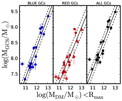
Again, the blue subpopulation reveals the tightest correlation but we also find that the scatter is significantly reduced from 0.26 to 0.20 dex when changing from a fixed spatial scale of 8 R_e to a matched spatial scale of R_max. This suggests that the mass in a GC system is strongly related to the enclosed dark matter mass. We have also examined the correlation of GC masses with total (i.e. dark plus stellar) mass and find the relations to have slightly more scatter than using the dark matter mass within R_max.

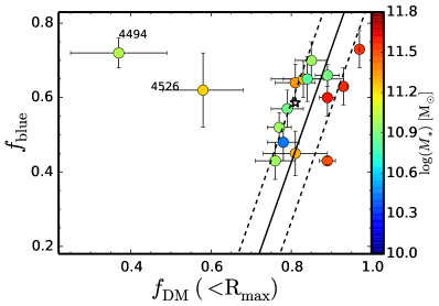
In Fig. 3 we show, for the first time, the metal–poor (blue) GC subpopulation fraction ( $f_{\rm blue}$ ) versus the fraction of dark matter ( $f_{\rm DM}$ ) enclosed within R_max, where $f_{\rm DM}=M_{\rm DM}/M_{\rm tot}$ . There is a strong correlation between $f_{\rm blue}$ and $f_{\rm DM}$ . The best fit to the data, excluding NGC 4494 and NGC 4526, is given in Table 3. Thus galaxies with GC systems that are dominated by blue GCs also have mass distributions that are dominated by dark matter.

None of the galaxies in the plot have blue GC fractions less than 0.4. The much larger sample of Harris et al. (2015) also reveals this to be the case (with one exception, for which the imaging does not cover the full GC system; W. Harris 2015, priv. comm.) Thus f_blue $>$ 0.4 may represent a minimum, or floor, in the blue GC fraction of galaxies. In contrast, the red GC fraction is known to be zero in some lower mass galaxies. From the best fit relation, f_blue $>$ 0.4 corresponds to a lower limit in the enclosed dark matter fraction of f_DM of 0.79. A typical blue GC fraction of 0.6 corresponds to an enclosed dark matter fraction of 0.86.

Table 3: Fit to blue globular cluster fraction with dark matter fraction (excluding NGC 4494 and NGC 4526)

	Slope	Intercept	rms
f_blue–f_DM within R_max	3.06 $\pm$ 1.28	–2.02 $\pm$ 1.11	0.16 $\pm$ 0.07

We also show in Fig. 3 the predicted blue GC fraction based on the findings of Harris et al. (2015). First, we estimate the halo mass for each galaxy in our sample using the M_∗–M_h relation of Behroozi et al. (2010). Next, we use the f_blue–M_h relation from Harris et al. to predict the blue GC fractions for our galaxies, given their halo mass (using eq. 3 of Harris et al.). In Fig. 3 we show this average predicted blue GC fraction versus the average enclosed dark matter fraction we measure for our sample (given by a star symbol). The predicted blue GC fraction agrees nicely with our empirical trend. The trend in Fig.3 also appears to be consistent with the GC systems of dwarf galaxies. Such galaxies are thought to be strongly dark matter dominated at large radii, and have blue GC fractions of approaching unity, i.e. they often contain no red GCs (Peng et al. 2008).

We now discuss the two deviant galaxies in Fig. 3 and whether their location in the plots might be spurious. Two effects may explain the deviation of NGC 4526 from the general trend. Firstly, it has the highest correction in our sample for kinematic substructure (Alabi et al. 2016). Uncorrected it would have $f_{\rm DM}$ ${\sim}0.7$ . It also had a fairly large correction applied by Peng et al. (2008) as the GC system is not fully covered by the ACS field-of-view, i.e. uncorrected $f_{\rm blue}$ = 0.48. If either of these corrections were not applied then NGC 4526 would be consistent within the errors with the general trend. Thus we suspect that NGC 4526 is not a true outlier and will obey the general trend with improved data.

NGC 4494 deviates most strongly from the general trend. Given that there appears to be a minimum, or floor, in the blue GC fraction of galaxies of f_blue $>$ 0.4, changes to the blue GC fraction will not place NGC 4494 on the general trend. So we turn our attention to its low dark matter fraction. Indeed we are not the first to find a low fraction of dark matter. Several studies using PNe to model the mass of NGC 4494 have derived a remarkably low dark matter content of $<$ 0.5 within 5 R_e (Romanowsky et al. 2003; Napolitano et al. 2009; Deason et al. 2012) However, the more recent NMAGIC modelling of the extended stellar kinematics (Foster et al. 2011) and the PNe data by Morganti et al. (2013) found a higher dark matter fraction of f_DM = 0.6 $\pm$ 0.1 within 5 R_e. They assumed a logarithmic potential for the dark matter rather than an NFW-type profile, which leads to a higher dark matter mass and a relatively low stellar mass-to-light ratio. The wide range of dark matter fractions in the literature suggest that NGC 4494 is difficult to model dynamically, and future mass modelling should attempt to incorporate stellar, PNe and GCs velocity information simultaneously. If NGC 4494 follows the general trends for blue GC total mass (Figures 1 and 2) and blue GC fraction (Figure 3) found in this work, then a significant dark mass and dark matter fraction is expected.

A possible explanation for the overall correlation seen in Fig. 3 is the process of halo growth via accretion of satellites. As galaxies accrete low-mass satellites they will also accrete dark matter and (preferentially) blue GCs. This tends to move a galaxy up and to the right in the plot. The data points in Fig. 3 have been coded by their stellar mass. In the two-phase model for galaxy formation (e.g. Oser et al. 2010), the fraction of accreted (ex-situ) stars is a strong function of stellar mass. The plot shows a weak secondary trend for the highest stellar mass galaxies to have the highest dark matter fraction for a given blue GC fraction. This suggests that the accretion of many low mass satellite galaxies gives rise to a high ratio of dark matter to blue GCs in the outer regions of the most massive galaxies (Amorisco 2015).

Alternatively, galaxies may move down and to the left in this plot via tidal stripping. For a typical galaxy in our sample the 2D surface density profile of a GC system has a power-law slope of –2. Assuming spherical symmetry this corresponds to –3 in 3D. At large radii an NFW profile slope is also around –3. Thus both the GC radial profile and that of the dark matter may follow a similar slope. This suggests that once tidal stripping has removed the outermost dark matter, further stripping would remove blue GCs (as they are more radially extended than the red subpopulation) and dark matter in roughly equal proportion. Tidal stripping of a galaxy with an initially high dark matter and blue GC fraction would move it down and parallel to the trend seen in Fig. 3. Thus both tidal stripping and halo growth via accretion may play a role in the correlation of blue GC fraction and enclosed dark matter fraction.

4 Conclusions

Using a sample of well-studied massive early-type galaxies, we compare the mass of their GC systems to the host galaxy’s dark matter content on similar spatial scales for the first time. We find a strong correlation between the mass of the blue (metal-poor) GC subpopulation and the dark matter content within a fixed 8 R_e. An even stronger correlation is found when the radius for calculating the dark matter mass is matched to the spatial scale of the GC system. Thus from careful imaging of a GC system, one can infer the enclosed dark matter mass to within a factor of two. The ratio of the GC system mass to that of the enclosed dark matter is nearly constant, and this can be understood in terms of the universal baryon fraction, the efficiency of GC formation and the radial profile of dark matter. We also find a tight correlation between the fraction of blue GCs and the enclosed dark matter fraction. GC systems appear to have a minimum blue fraction of 40 per cent, although a typical galaxy, with blue GC fraction of 60 per cent, has 86 per cent of its mass in dark matter (and 14 per cent in stars). The dark matter mass of NGC 4494 has been debated in the literature, but based on our findings we support claims that it is heavy with dark matter. Both halo growth and removal (via tidal stripping) may play some role in shaping this trend. We suggest that galaxies with the highest accretion fractions reveal higher dark matter fractions for a given blue GC fraction.

5 Acknowledgements

We thank J. Janz for useful discussion and the referee, Bill Harris, for his helpful suggestions. DAF thanks the ARC for financial support via DP130100388. This work was supported by NSF grant AST-1211995.

6 References

Alabi A., et al. 2016, in prep.
Amorisco, N., 2015, arXiv:1511.08806
Behroozi P. S., Conroy C., Wechsler R. H., 2010, ApJ, 717, 379
Blakeslee J. P., Tonry J. L., Metzger M. R., 1997, AJ, 114, 482
Blom C., Spitler L. R., Forbes D. A., 2012, MNRAS, 420, 37
Brodie J. P., Usher C., Conroy C., Strader J., Arnold J. A., Forbes D. A., Romanowsky A. J., 2012, ApJ, 759, L33
Brodie J. P., et al., 2014, ApJ, 796, 52
Diemand J., Madau P., Moore B., 2005, MNRAS, 364, 367
Diemer B., More S., Kravtsov A. V., 2013, ApJ, 766, 25
Durrell P. R., et al., 2014, ApJ, 794, 103
Faifer F. R., et al., 2011, MNRAS, 416, 155
Forbes D. A., 2005, ApJ, 635, L137
Forbes D. A., Spitler L. R., Strader J., Romanowsky A. J., Brodie J. P., Foster C., 2011, MNRAS, 413, 2943
Forbes D. A., Ponman T., O’Sullivan E., 2012, MNRAS, 425, 66
Forbes D. A., Pastorello N., Romanowsky A. J., Usher C., Brodie J. P., Strader J., 2015, MNRAS, 452, 1045
Forte J. C., Faifer F., Geisler D., 2007, MNRAS, 382, 1947
Forte J. C., Vega E. I., Faifer F. R., Smith Castelli A. V., Escudero C., González N. M., Sesto L., 2014, MNRAS, 441, 1391
Foster C., et al., 2011, MNRAS, 415, 3393
Georgiev I. Y., Puzia T. H., Goudfrooij P., Hilker M., 2010, MNRAS, 406, 1967
Guo Q., et al., 2010, MNRAS, 404, 1111
Harris W. E., 2009, ApJ, 699, 254
Harris W. E., Harris G. L. H., Alessi M., 2013, ApJ, 772, 82
Harris W. E., Harris G. L., Hudson M. J., 2015, ApJ, 806, 36
Hudson M. J., Harris G. L., Harris W. E., 2014, ApJ, 787, L5
Kartha S. S., Forbes D. A., Spitler L. R., Romanowsky A. J., Arnold J. A., Brodie J. P., 2014, MNRAS, 437, 273
Kartha S., et al. 2015, MNRAS, submitted
Katz H., Ricotti M., 2014, MNRAS, 444, 2377
Kavelaars J. J., 1999, ASPC, 182, 437
Kravtsov A. V., Gnedin O. Y., 2005, ApJ, 623, 650
McLaughlin D. E., 1999, AJ, 117, 2398
Morganti L., Gerhard O., Coccato L., Martinez-Valpuesta I., Arnaboldi M., 2013, MNRAS, 431, 3570
Napolitano N. R., et al., 2009, MNRAS, 393, 329
Oser L., Ostriker J. P., Naab T., Johansson P. H., Burkert A., 2010, ApJ, 725, 2312
Peng E. W., et al., 2008, ApJ, 681, 197
Pota V., et al., 2013, MNRAS, 428, 389
Romanowsky A. J., Douglas N. G., Arnaboldi M., Kuijken K., Merrifield M. R., Napolitano N. R., Capaccioli M., Freeman K. C., 2003, Sci, 301, 1696
Spitler L. R., Forbes D. A., Strader J., Brodie J. P., Gallagher J. S., 2008, MNRAS, 385, 361
Spitler L. R., Forbes D. A., 2009, MNRAS, 392, L1
Usher C., et al., 2012, MNRAS, 426, 1475
Usher C., Forbes D. A., Spitler L. R., Brodie J. P., Romanowsky A. J., Strader J., Woodley K. A., 2013, MNRAS, 436, 1172
Watkins L. L., Evans N. W., An J. H., 2010, MNRAS, 406, 264