$A$-expansion for multiple “hedgehog” shapes

Abstract

Overlapping colors and cluttered or weak edges are common segmentation problems requiring additional regularization. For example, star-convexity is popular for interactive single object segmentation due to simplicity and amenability to exact graph cut optimization. This paper proposes an approach to multi-object segmentation where objects could be restricted to separate “hedgehog” shapes. We show that $\alpha$-expansion moves are submodular for our multi-shape constraints. Each “hedgehog” shape has its surface normals constrained by some vector field, e.g. gradients of a distance transform for user scribbles. Tight constraint give an extreme case of a shape prior enforcing skeleton consistency with the scribbles. Wider cones of allowed normals gives more relaxed hedgehog shapes. A single click and $\pm 90^{\circ}$ normal orientation constraints reduce our hedgehog prior to star-convexity. If all hedgehogs come from single clicks then our approach defines multi-star prior. Our general method has significantly more applications than standard one-star segmentation. For example, in medical data we can separate multiple non-star organs with similar appearances and weak or noisy edges.

1 Introduction

Distinct intensity appearances and smooth contrast-aligned boundaries are standard segmentation cues. However, in most real applications of image segmentation there are multiple objects of interest with similar or overlapping color appearances. Intensity edges also could be cluttered or weak. These common practical problems require additional regularization, as illustrated in the second row of Figure 1.

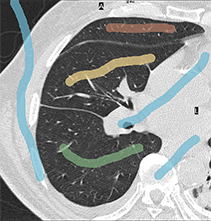
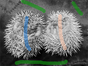
two examples of images with seeds (medical and photo)
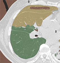
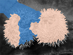
multi-object segmentation using Potts model
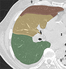
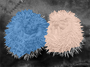
multi-object segmentation adding our hedgehog shapes prior

Figure 1: Hedgehog shapes prior for multi-object segmentation.

There are multiple methodologies for enforcing shape regularity or shape priors. For example, Statistical Shape Models (SSM) [26, 6, 1] and Deformable Shape Models (DSM) [17] differ in their shape space representation and their distance measures between a given segmentation and the learned shape space. SSM applies principal component analysis to a training dataset for fitting the shape space distribution represented by a mean shape and the modes of greatest variance. Any given segmentation could be penalized based on how well it aligns to this shape space [26] or it could be restricted to the learned shape space [6]. M-rep [17] is a coarse-to-fine discrete DSM approach. In contrast to basic user-scribbles like in our method, M-reps requires detailed user inputs defining a figural shape model for each segment. They also need training data to estimate their model parameters. SSM and DSM assume a fixed shape topology, which is often violated by specific problem instances, e.g. lesions, tumors, or horse-shoe kidneys [23].

Our paper proposes a simple and sufficiently general shape regularization constraint that could be easily integrated into standard MRF methods for segmentation. Shape priors have been successfully used in binary graph cut segmentation [14, 25, 10]. While our “hedgehog” shape prior is a generalization of the popular star-convexity constraint [25] with several merits over previous extensions [14, 10], our main contribution is a multi-hedgehog prior in the context of multi-object segmentation problems.

We observe that similarity between object appearances and edge clutter are particularly problematic in larger multi-label segmentation problems, e.g. in medical imaging. Our multi-hedgehog prior is fairly flexible, has efficient optimizers, and shows significant potential in resolving very common ambiguities in multi-label segmentation problems, see Fig.1 (last row). Our general multi-object segmentation framework allows to enforce “hedgehog” shape prior for any of the objects. The class of all possible hedgehog priors is sufficiently representative yet each specific hedgehog constraint offers sufficient regularization to address color overlap and weak/cluttered edges. One extreme case of our prior is closely related to the standard star shape prior [25]. The other extreme case allows shapes with restricted skeletons [18, 24].

The main contribution of our work is a practical and efficient way to combine distinct shape priors for segments in popular multi-label MRF framework [5]. Our work also allows to extend previous multi-surface graph cut methods [16, 7]. For example, [16] compute multiple nested segments using one fixed polar grid defined by some non-overlapping rays. Besides particular image discretization, these rays introduce two constraints: one star-like shape constraint shared by the nested segments and a smoothness constraint penalizing segment boundary jumping between adjacent rays. In contrast, our method defines independent shape constraints for each segment. Similarly to [14], shape normals are constrained by arbitrary vector fields, rather than non-overlapping rays [16] or trees [25, 10]. Our use of Cartesian grid allows to enforce standard boundary length smoothness [3]. While this paper is focused on a Potts model with distinct shape constrains, hedgehog shapes can be easily combined with inter-segment inclusion or exclusion constraints [7]. The use of distinct (not necessarily nested) shape priors extends the range of applications in [16].

Our Potts framework optimization algorithm is closely comparable with a special non-submodular case of [7] with exclusion constraints. While we use independent shape constrains for each segment, these are easy to integrate into each layer in [7]. More importantly, instead of binary multi-layer formulation with non-submodular potentials, we use multi-label formulation amenable to $\alpha$-expansion. Besides memory savings, our approach solves the non-submodular segmentation problem with a guaranteed approximation quality bound. Section 4 discusses relations to [16, 7] in more details.

Overview of contributions: We propose a new multi-label segmentation model and the corresponding optimization algorithm. Our contributions are summarized below.

• hedgehog shape constraint - a new flexible method for segment regularization based on simple and intuitive user interactions.

• new multi-object segmentation energy with multi-hedgehog shape priors.

• we provide an extension of $\alpha$-expansion moves [5] for the proposed energy.

• experimental evaluation showing how our multi-object segmentation method solves problematic cases for the standard Potts model [5].

The rest of the paper is organized as follows. Section 2 defines our hedgehog shape prior for a simpler case of binary segmentation of one object. We discuss its properties and show how it can be globally optimized with $s/t$ graph cuts. Section 3 defines multi-hedgehog shape constraint in the context of multi-label MRF segmentation and proposes an extension of $\alpha$-expansion optimization algorithm. Our experiments in Section includes multi-object segmentation of real photos and 3D multi-modal medical data.

2 Hedgehog shape constraint for one object

This section describes our hedgehog shape prior for a single object in case of binary segmentation. Section 3 describes a more general multi-hedgehog segmentation prior where multiple objects can have separate hedgehog constraints. While multi-hedgehog prior helps in a much wider range of problems, e.g. in medical imaging, binary segmentation with one “hedgehog” is easier to start from and it has merits on its own. In particular, single-hedgehog prior generalizes popular star-convexity [25] differently from other related methods [14, 10] in binary segmentation.

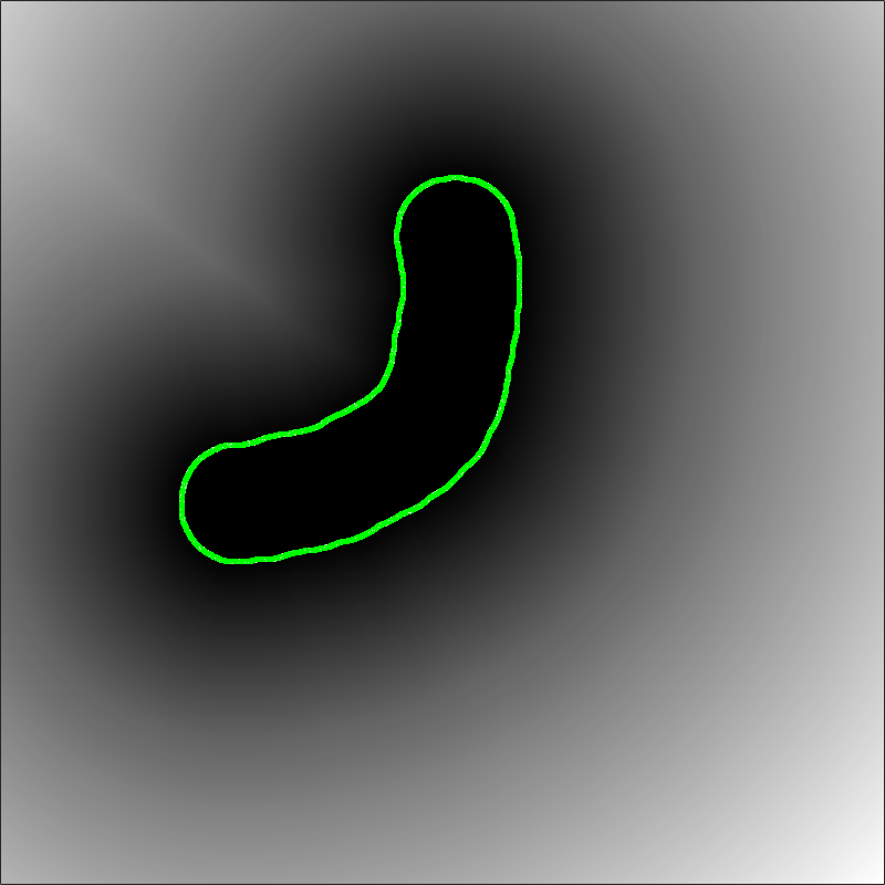
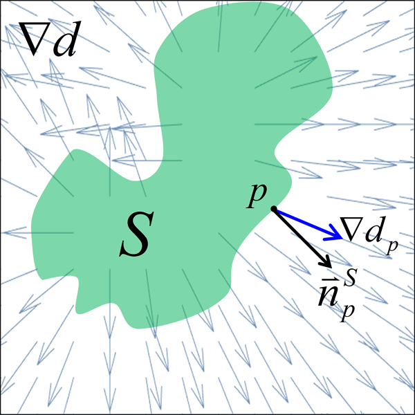
(a) scribble’s distance map $d$	(b) constraint $\angle({\bar{n}}^{S}_{p},\nabla d_{p})\leq\theta$

Figure 2: Hedgehog prior for segment $S$. (a) User-scribble or shape template define a (signed) distance map $d$. (b): Orientations of surface normals ${\bar{n}}^{S}_{p}$ for $S$ are constrained by $\angle({\bar{n}}^{S}_{p},\nabla d_{p})\leq\theta$.

Similarly to star prior [25], hedgehog prior could be defined interactively. Instead of a single click in the star center, hedgehog shape allows an arbitrary scribble roughly corresponding to its skeleton. Hedgehog can also be defined by an approximate user-defined outline of a desired shape or by a shape template. In any case, such scribble, outline, or template define the corresponding (signed) distance transform or distance map $d:\Omega\rightarrow{\mathcal{R}}$ and a field of its gradients $\nabla d$, as illustrated in Fig.2. Our hedgehog constraint for segment $S$ is defined by vector field $\{\nabla d_{p}\;|\;p\in\Omega\}$ and angular threshold $\theta$ restricting orientations of surface normals ${\bar{n}}^{S}_{p}$ at any point $p$ on the boundary of $S$ to a cone

$$C_{\theta}(p):\;\;\;\;\;\angle({\bar{n}}^{S}_{p},\nabla d_{p})\leq\theta\;\;\;\;\;\;\;\;\forall p\in\partial S$$ (1)

assuming gradient $\nabla d_{p}$ is defined at $p$. More generally, hedgehog constraint for segment $S$ could be defined by any given vector field $\{{\bar{v}}_{p}\;|\;p\in\Omega\}$ defining preferred directions for surface normals. Similarly to [14], we can use dot product to define allowed normals cones $C_{\theta}(p):\;\langle{\bar{n}}^{S}_{p},{\bar{v}}_{p}\rangle\geq\tau$ where width varies depending on the magnitude of ${\bar{v}}_{p}$. In case ${\bar{v}}_{p}=\nabla d_{p}$ this constraint reduces to (1) for $\tau=cos(\theta)$ since $|\nabla d_{p}|=1$ at all points where gradient $\nabla d_{p}$ exists.

2.1 Single hedgehog properties

Even a single hedgehog shape prior discussed in this section could be useful in practice. For example, if $\theta=\pi/2$ it closely approximates a popular star convexity [25] in case of a single click. However, our formulation uses locally defined constraints, which can be approximated by a simple rule for selecting local edges, see Section 2.2. Unlike [25], we do not enforce a global tree structure, see Fig.3(b). Also, like [14, 10] hedgehog prior allows a much larger variability of shapes for scribbles different from a point. In our case, a scribble defines a rough skeleton of a shape. For example, for smaller values of $\theta$ our cone constraints (1) give a tighter alignment of surface normals with vectors $\nabla d_{p}$ forcing the segment boundary to closely follow the level-sets of the scribble’s distance map $d$, see Fig.5. In the limit, this implies consistency of segment’s skeleton with the skeleton of the given scribble, outline, or template.

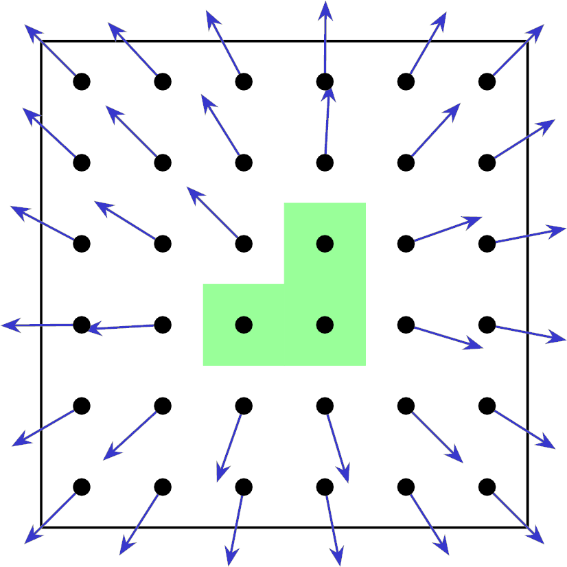
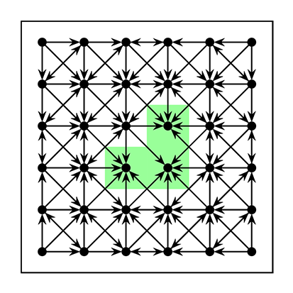
(a) gradients $\nabla d$	(b) graph edges $\mathcal{E}(0)$
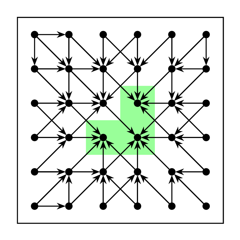
(c) graph edges $\mathcal{E}(\frac{\pi}{4})$	(d) graph edges $\mathcal{E}(\frac{3\pi}{8})$

Figure 3: Hedgehog constraint (1) for user seeds (green) and the corresponding distance map gradients $\nabla d$ in (a) is approximated by infinity cost directed edges $\mathcal{E}(\theta)$ in (b-d) selected as in Fig.4.

2.2 Single hedgehog via graph cuts

We show an approximation for hedgehog constraint (1) for object $S$ in the context of binary N-dimensional image segmentation via graph cuts [2]. All cone constraints (1) for any given $\theta$ and distance map gradients $\nabla d$, see Fig.3(a), correspond to a certain set of infinity cost directed edges, see Fig.3(b-d). For example, consider cone of allowed surface normals $C_{\theta}(p)$ at some point $p$ illustrated in Fig.4 for two different values of parameter $\theta$. It is easy to see that a surface/boundary of segment $S$ passing at $p$ has normal ${\bar{n}}^{S}_{p}\in C_{\theta}(p)$ iff this surface does not cross the corresponding polar cone

$${\hat{C}}_{\theta}(p)\;:=\;\{(py)\,|\,\langle(py),(pz)\rangle\leq 0\;\;\forall z\in C_{\theta}(p)\}.$$ (2)

This reformulation of our hedgehog constraint (1) is easy to approximate via graph cuts by setting infinity cost to all directed edges adjacent to $p$ whose directions agrees with polar cone ${\hat{C}}_{\theta}(p)$, see Fig.4. To avoid clutter, the figure only shows such directed edges $(pq)\in{\hat{C}}_{\theta}(p)$ starting at $p$, but one should also include similarly oriented directed edges $(qp)\in-{\hat{C}}_{\theta}(p):=\{(yp)\,|\,\langle(yp),(pz)\rangle\leq 0\;\;\forall z\in C_{\theta}(p)\}$ pointing to $p$. The set of all directed graph edges consistent with local polar cones orientations, see Fig.3(b-d), is

$$\!\!\!\!\mathcal{E}(\theta)\!=\!\{(pq)\in\mathcal{N}\;|\;(pq)\in\hat{C}_{\theta}(p)\;or\;(pq)\in-\hat{C}_{\theta}(q)\}.$$ (3)

Obviously, hedgehog constraints are better approximated by larger neighborhood systems $\mathcal{N}$, e.g. 32-neighborhood works better than 8-neighborhood, see Fig.5(b,c).

The used vector field has a direct effect on the set of allowed shapes when varying $\theta$. Figure 6 shows the segmentation result for varying $\theta$ for two different vector fields on the same synthetic example.

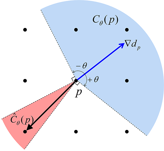
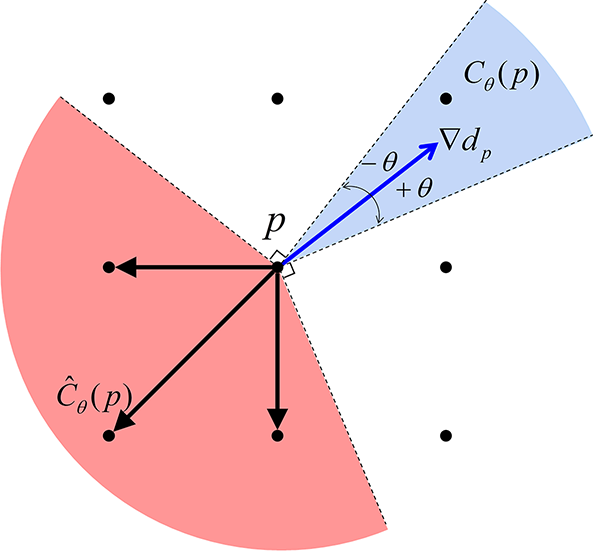
(a) wide cone of normals $C_{\theta}$	(b) tight cone of normals $C_{\theta}$

Figure 4: Approximating hedgehog constraint (1) at grid node $p$. Cone $C_{\theta}$ of allowed surface normals (blue) is enforced by $\infty$ cost directed edges $(pq)$ in the corresponding polar cone ${\hat{C}}_{\theta}$ (red).

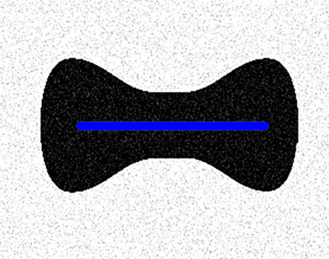
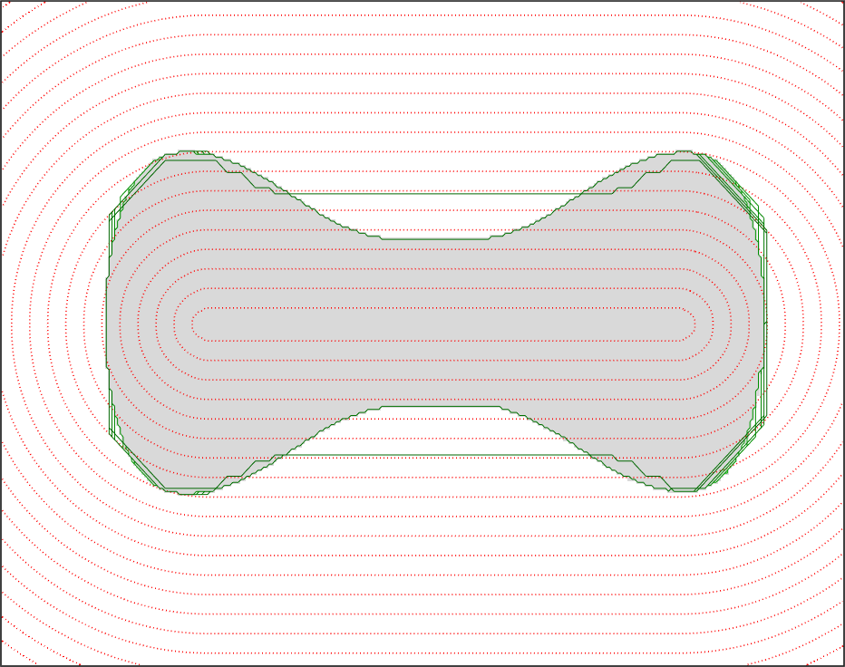
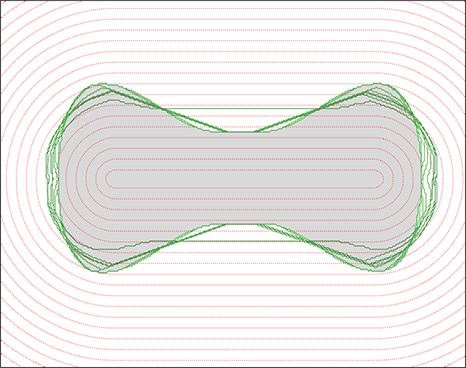
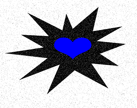
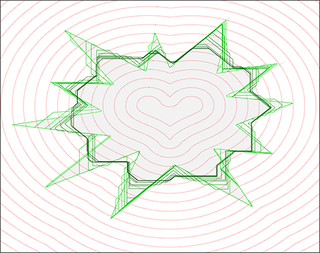
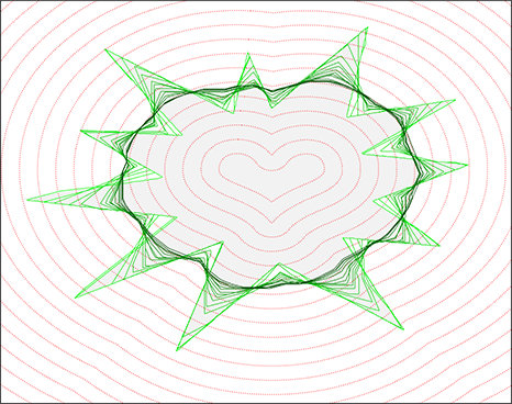
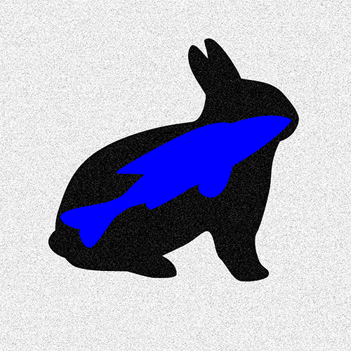
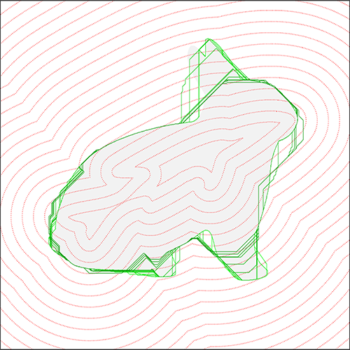
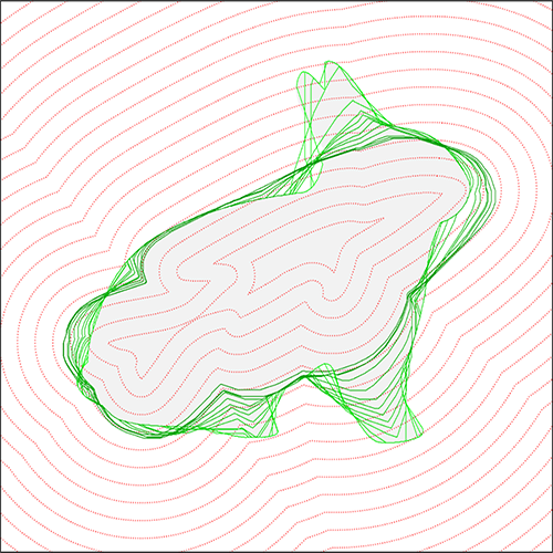
(a) image and user scribble (blue)	(b) 8-neighborhood	(c) 32-neighborhood

Figure 5: Single hedgehog shape constraint (1) for different parameters $\theta$. User scribbles in (a) define distance map $d$ and, consequently, vector field $\nabla d$ in (1). Red contours in (b,c) are level sets of distance map $d$. Green contours show optimal graph cut segmentation (Sec.2.2) using hedgehog constrains with different values of parameter $\theta$ in the range $[0,\frac{\pi}{2}]$. In these synthetic examples the object boundary nearly satisfies our hedgehog constraint for $\theta=\frac{\pi}{2}$. However, smaller parameters $\theta$ (darker green contours) correspond to tighter constraints for segment normals, see Fig.4, forcing object and background segments to deviate from their given color models. As $\theta$ approaches $0$, constraint (1) closely aligns segments with level sets of $d$ (skeleton consistency). Discretization artifacts decrease for larger $\mathcal{N}$, see (c).

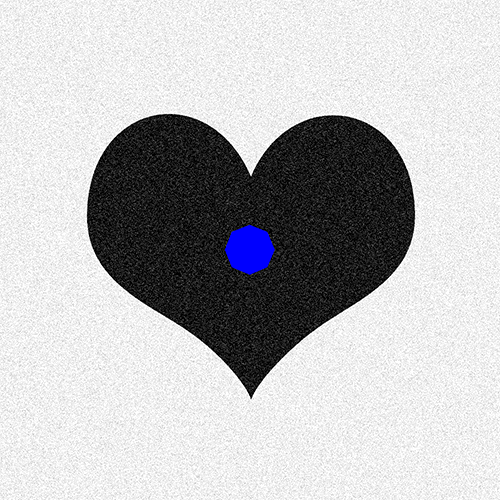
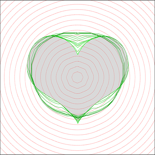
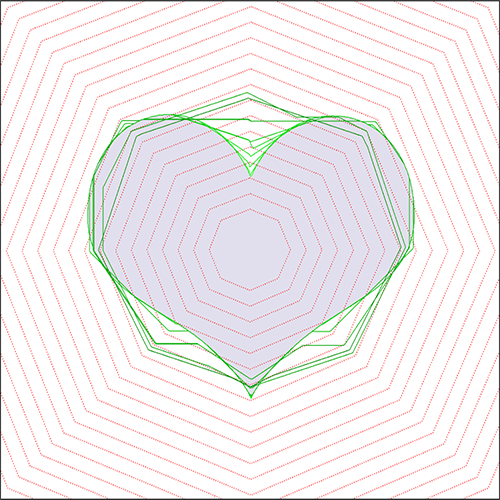
(a) image and user scribble (blue)	(b) Euclidean Distance Transform gradient	(c) synthetic vector field

Figure 6: Single hedgehog shape constraint (1) for different parameters $\theta$ and different vector fields. (a) image and scribble (octagon shown in blue). (b-c) show our results for varying $\theta$, ground truth (shown in gray) and the vector field used to enforce hedgehog constraints (shown in blue). In (b) the vector field is the Euclidean Distance Transform gradient of the user-scribble and in (c) it is the gradient of a function where the level-sets are scaled versions of the scribble. Notice how the used vector field affects the segmentation for the same value of $\theta$ in (b) and (c).

It is easy to see that set (3) of infinity cost edges corresponds to a submodular pairwise energy approximating hedgehog shape constraint (1) for binary labeling $\mathbf{f}=\{f_{p}\}$ representing segment $S=\{p\;|\;f_{p}=1\}$

$$h_{\theta}(\mathbf{f})\;=\;\sum_{(pq)\in\mathcal{E}(\theta)}w_{\infty}\cdot[f_{p}=1,f_{q}=0]$$ (4)

where $w_{\infty}$ is an infinitely large scalar.

3 Multi-hedgehog segmentation energy

Given a set of pixels $\mathcal{P}$, neighborhood system $\mathcal{N}$, and labels $\mathcal{L}$ our multi-labeling segmentation energy is

$$E(\mathbf{f})=\overbrace{\sum_{p\in\mathcal{P}}D_{p}(f_{p})}^{\text{\small{\em data}}}+\overbrace{\lambda\!\!\sum_{pq\in\mathcal{N}}V_{pq}(f_{p},f_{q})}^{\text{\small{\em smoothness}}}+\overbrace{\vphantom{\sum}H_{\theta}(\mathbf{f})}^{\text{\small{\em hedgehogs}}}$$ (5)

where $\mathbf{f}=\{f_{p}\in\mathcal{L}|\;\forall p\in\mathcal{P}\}$ is a labeling.

The first two terms, namely data and smoothness terms, are widely used in computer vision, e.g. [4, 2, 19]. The data term commonly referred to as the regional term as it measures how well pixels fit into their corresponding labels. To be specific, $D_{p}(f_{p}$) is the penalty for assigning label $f_{p}$ to pixel $p$. Similar to [19], a label’s probabilistic model, a Gaussian Mixture in our case, is found by fitting a probabilistic model to the seeds given by the user.

The smoothness term is a standard pairwise regularizer that discourages segmentation discontinuities between neighboring pixels. A discontinuity occurs whenever two neighboring pixels $pq\in\mathcal{N}$ are assigned to different labels. In its simplest form, $V_{pq}(f_{p},f_{q})=w_{pq}[f_{p}\neq f_{q}]$ where $[\;]$ is Iverson bracket and $w_{pq}$ is a non-increasing function of the intensities at $p$ and $q$. Also, $\lambda$ is a parameter that weights the importance of the smoothness term.

Third term, our contribution, is the Hedgehog term

$$H_{\theta}(\mathbf{f})=\sum_{k\in\mathcal{L}}\sum_{\;(pq)\in\mathcal{E}_{k}(\theta)}\!\!\!w_{\infty}\;[f_{p}=k,f_{q}\neq k]$$ (6)

where $w_{\infty}=\infty$. Those familiar with graph cuts may prefer to think of it as an $\infty$-cost arc from $p$ to $q$, thus prohibiting any cut that satisfy $f_{p}=k$ and $f_{q}\neq k$.

The Hedgehog term is the sum of the Hedgehog constraints over all the labels and it guarantees that any feasible labeling, i.e. $E(\mathbf{f})<\infty$, will result in a segmentation with surface normals respecting the orientation constraints (1). Notice that (6) reduces to [25] when $\theta=90^{\circ}$, $|\mathcal{L}|=2$ and the shape constraints are defined for only one of the labels by a single pixel.

3.1 Expansion Moves

In this section we will describe how to extend the binary expansion moves of $\alpha$-exp [5] to respect the shape constraints, and show that these moves are submodular. The main idea of $\alpha$-exp algorithm is to maintain a current feasible labeling $\mathbf{f}^{{}^{\prime}}\!\!$, i.e. $E(\mathbf{f}^{{}^{\prime}})\!\!<\!\!\infty$, and iteratively move to a better labeling until no improvements could be made. To be specific at each iteration, a label $\alpha\in\mathcal{L}$ is chosen and variables $f_{p}$ for all $p\in\mathcal{P}$ are given a binary choice $x_{p}$; 0 to retain their old label $f_{p}=f^{{}^{\prime}}_{p}$ or 1 switch to $\alpha$, i.e. $f_{p}=\alpha$.

The Hedgehog term (6) for a binary $\alpha$-exp move could be written as

$$H^{\alpha}_{\theta}(\mathbf{x})=\!\!\!\sum_{\!\!\!\!\!\!\!\!\!\!(p,q)\in\mathcal{E}_{\alpha}(\theta)}\!\!\!S_{pq}(x_{p},x_{q})+\!\!\!\!\sum_{k\in\mathcal{L}\setminus\alpha}\!\underset{\begin{subarray}{c}f^{{}^{\prime}}_{p}=f^{{}^{\prime}}_{q}=k\\ \\ (pq)\in\mathcal{E}_{k}(\theta)\end{subarray}}{\sum}\!\!\!\!\!\!\!S_{qp}(x_{q},x_{p})$$ (7)

where $\mathbf{x}=\{x_{p}\in\{0,1\}\;|\;\forall p\in\mathcal{P}\}$ and

$$S_{pq}(x_{p},x_{q})=\left\{\begin{tabular}[]{cc}$\infty$&if $x_{p}=1,\;x_{q}=0$\\ 0&\text{otherwise.}\end{tabular}\right.$$ (8)

The first term in (7) guarantees that the resulting labeling respects label $\alpha$ hedgehog constraints. In addition, the second term guarantees that the hedgehog constraints satisfied by the current labeling $\mathbf{f}^{{}^{\prime}}$ for all labels in $\mathcal{L}\setminus\alpha$ are not violated by the new labeling $\mathbf{f}$.

According to [15], any first-order binary function could be exactly optimized if all pairwise terms are submodular. A binary function $g$ of two variables is submodular if $g(0,0)+g(1,1)\leq g(1,0)+g(0,1)$. Our energy (7) is submodular as it could be written as the sum of submodular pairwise binary energies over all possible pairs of $p$ and $q$. Notice that for any given $pq$ pair, $S_{pq}(1,1)=0$ by construction and $S_{pq}(0,0)=0$ as long as the current labeling is a feasible one, i.e. it does not cut any of the $\infty$-cost arcs. Also, $S_{pq}(1,0)$ and $S_{pq}(0,1)$ are both $\geq 0$ by construction. Therefore, the submodularity condition is satisfied for all pairs of $p$ and $q$.

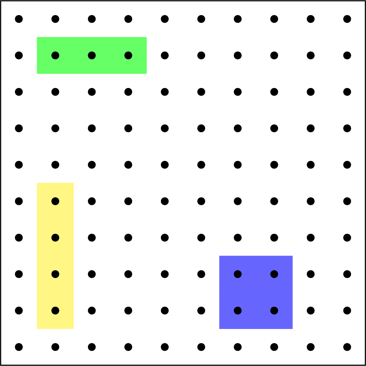
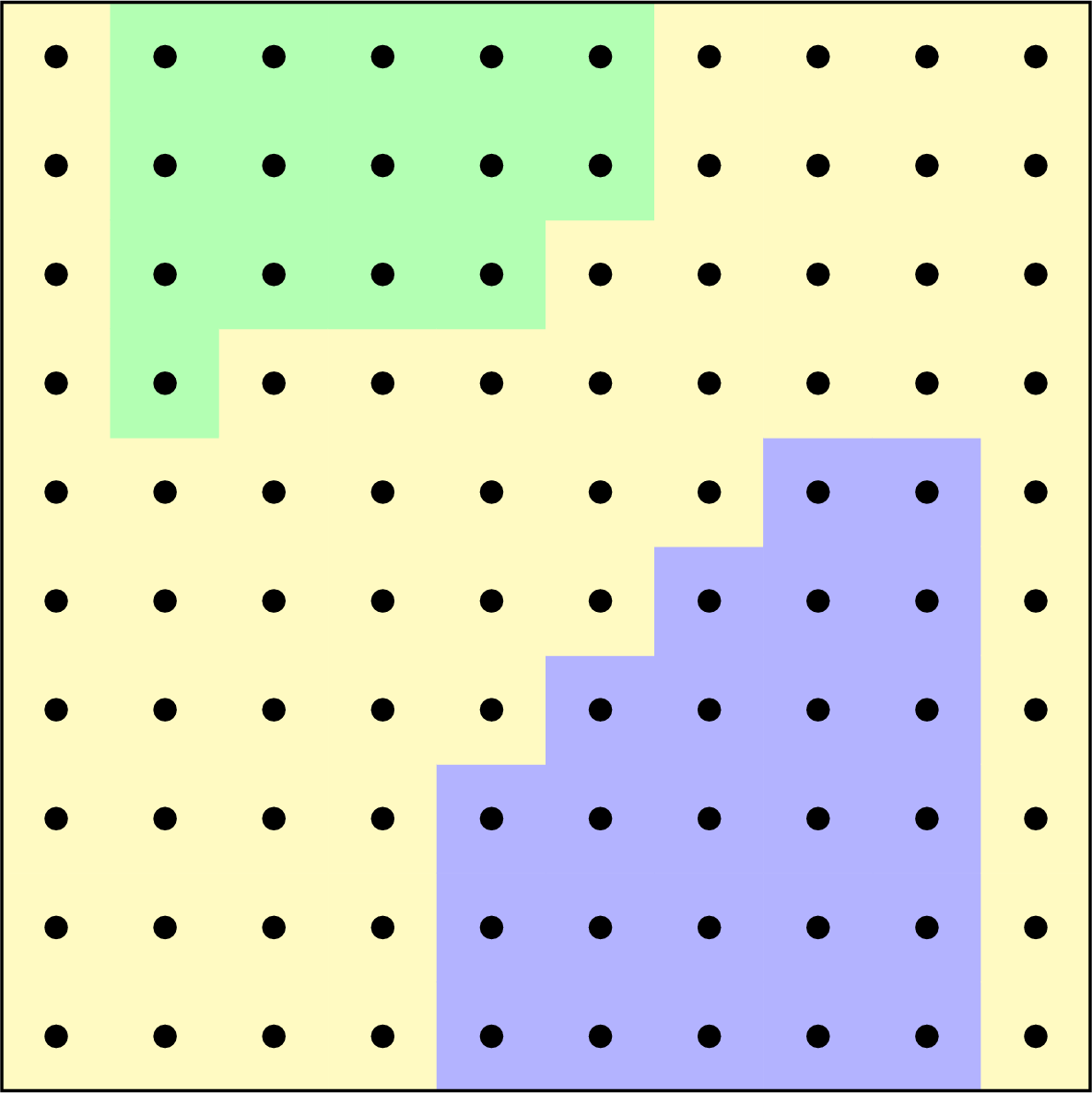
(a) initial Seeds	(b) current labeling
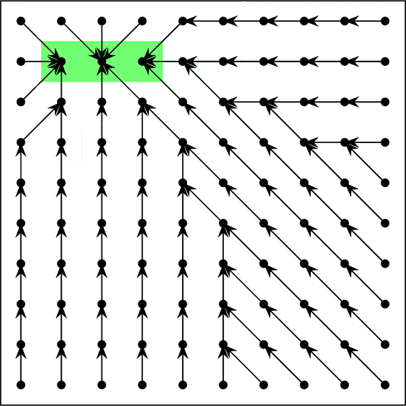
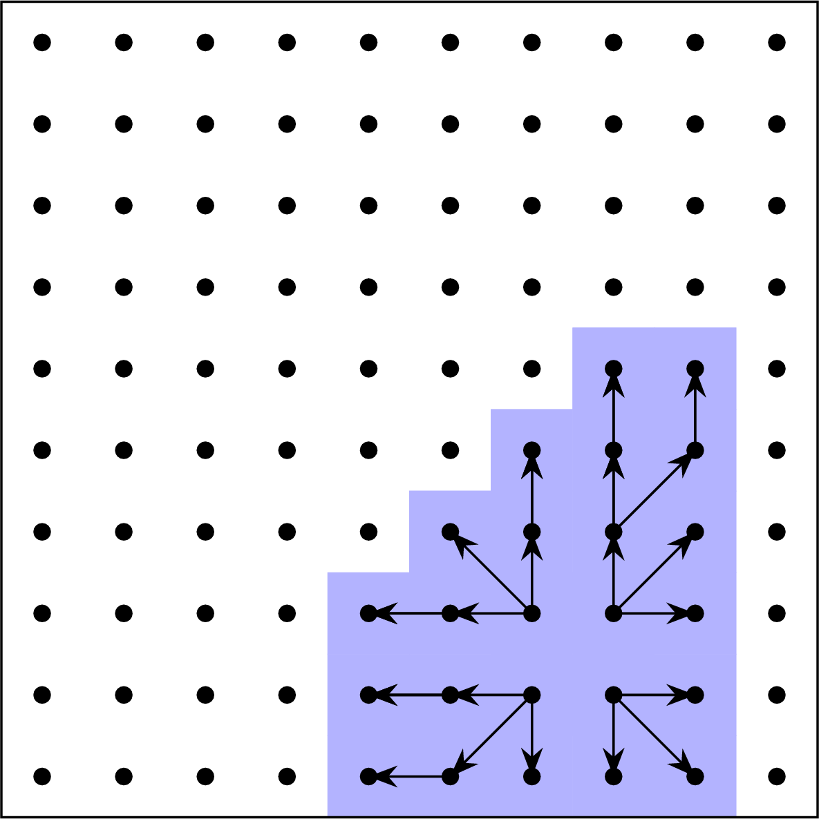
(c) (7) first term constraints	(d) (7) second term constraints
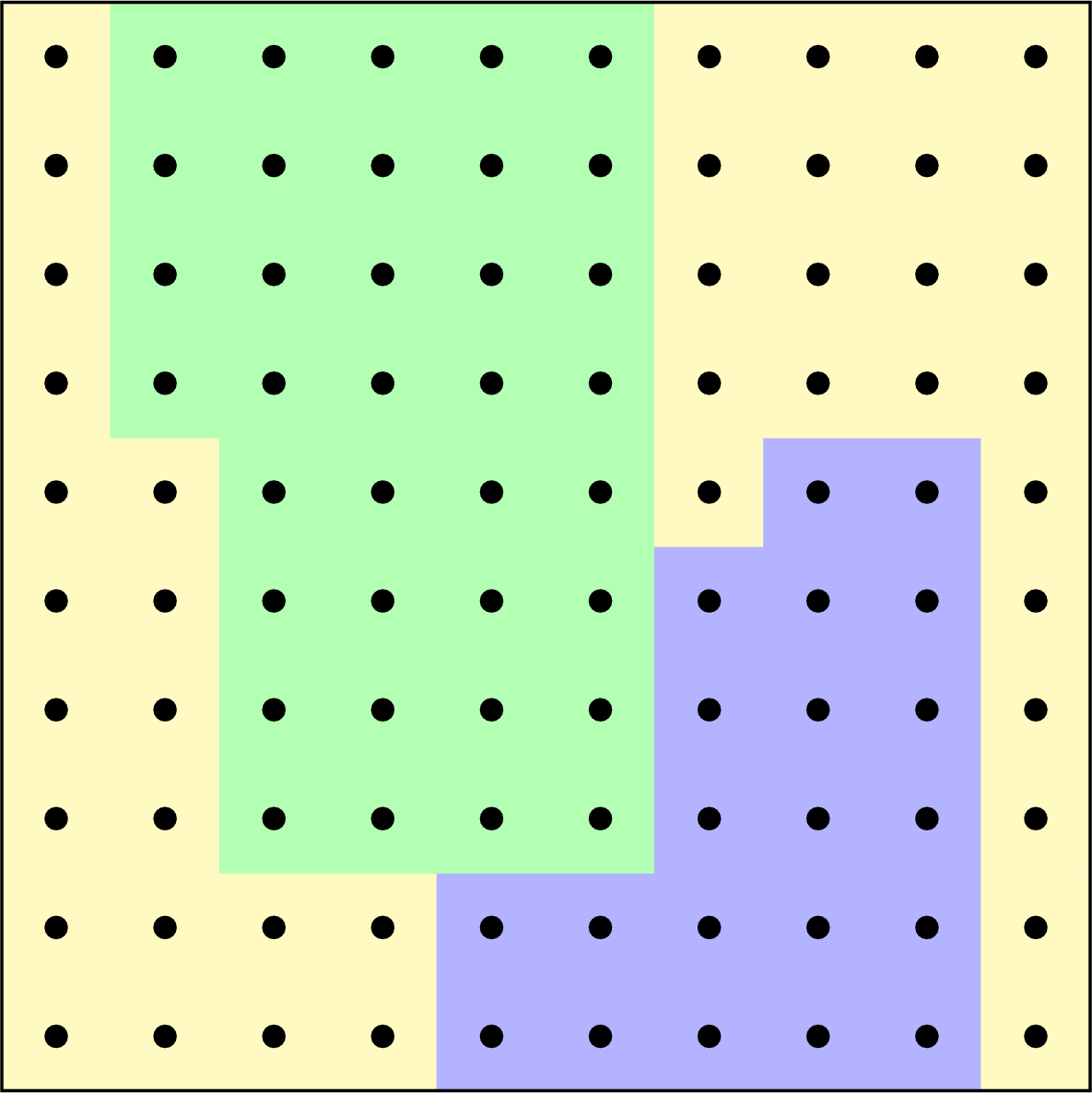
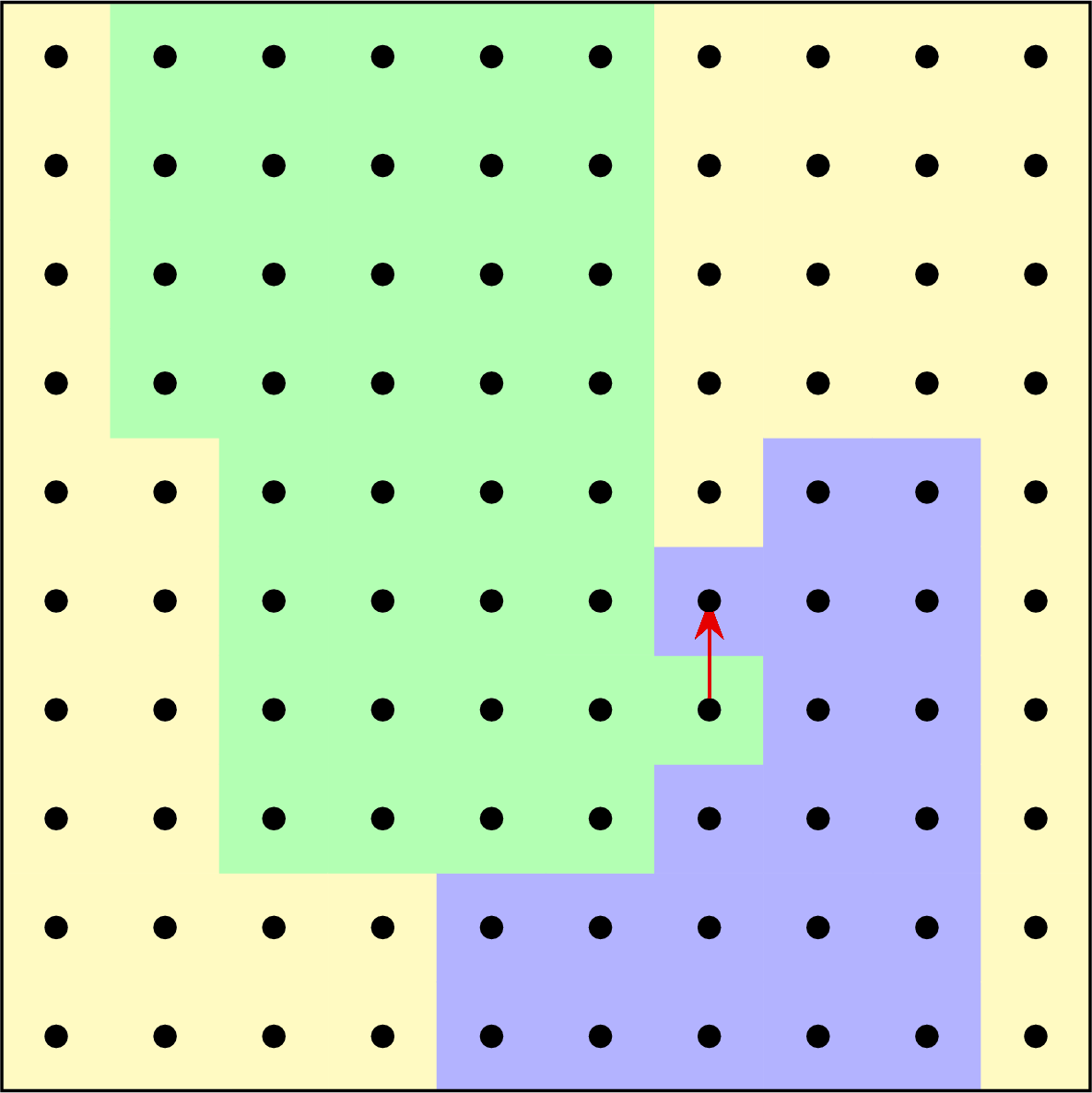
(e) feasible expansion move	(f) infeasible expansion move

Figure 7: Illustration of a feasible and an infeasible expansion move for the green label. (a-b) Initial seeds and current labeling, respectively. (c-d) Hedgehog shape constraints (7) enforced by green and purple labels when expanding the green one. (e-f) show a feasible and an infeasible expansion moves, respectively. In (f) severed $\infty$-cost purple shape edge/constraint is shown in red.

Fig.7 shows an example of an $\alpha$-exp move over the green label. We assume the shape constraints only for the green and purple labels. Fig.7(a) shows the initial seeds for three different labels while (b) shows the current feasible labeling. Fig.7(c-d) show the shape constraints enforced by green and purple labels while expanding the green label. Note, the green shape constraints are enforced all over the image while the purple shape constraints are enforced inside its current labeling support area, as it is not necessarily to enforce it everywhere. Fig.7(e) shows a feasible move that respects the green and purple shape constraints while (f) shows an infeasible move that respects only the green shape constraints.

4 Relation to multi-surface graph cuts

Our work could be related to multi-object segmentation methods [16, 7] combining various forms of boundary regularization and interactions between the surfaces. In particular, Logismos [16] computes nested segments using polar grid layers (one per segment) as in Fig.8(b). In general, edges between the layers enforce inter-surface constraints like minimum and maximum distances between the surfaces along each ray. For these constraints to work, the polar grids should be the same at all layers. Edges within each polar grid enforce regularity of the corresponding segment. Figure 8(b) details the construction. Red edges penalize inter-ray surface jumps and infinity cost green edges enforce a shape prior analogous to star convexity [25].

Cartesian discretization approach	polar discretization approach
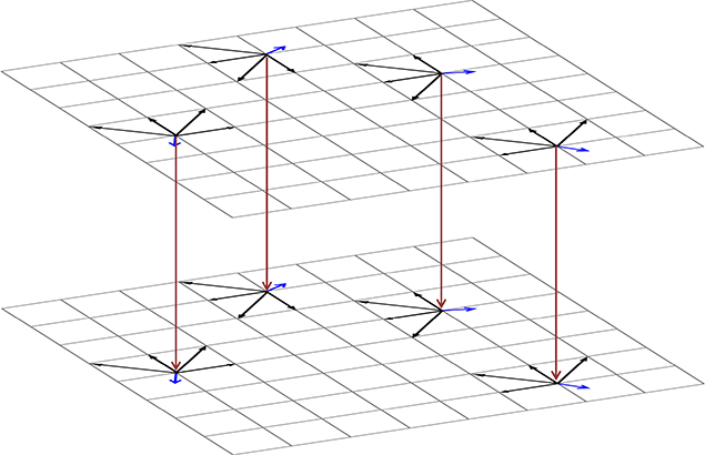
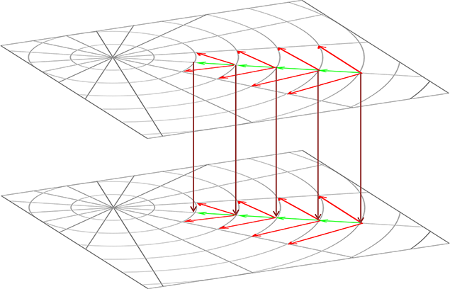
(a) Two identical hedgehogs with inclusion constraint [7]	(b) Two identical nested stars as in Logismos [16]
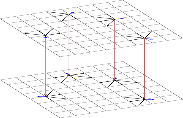
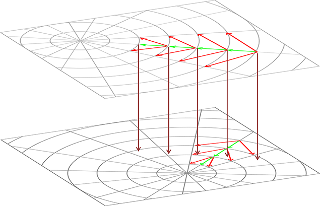
(c) Two distinct hedgehogs with inclusion constraint [7]	(d) Extended multi-polar Logismos with distinct stars

Figure 8: Multi-object graph cut methods [16, 7] with similar inter-surface constraints and shape priors. Each object corresponds to a layer. The shown inter-layer (brown) edges represent the simplest examples of inter-surface constraints, i.e.  inclusion with zero margin [7] in (a,c) and nestedness with zero min distance [16] in (b,d). While, the standard regularization of each layer segment in [7] is its boundary length [3], it can be easily complemented or replaced by shape priors like star [25] or our hedgehog. Integrating the same hedgehog shape (black edges, as in Fig.4) into both layers (a) creates a Cartesian analogue of Logismos [16] (b) based on a vector field (blue) instead of non-overlapping rays. Using distinct hedgehog shapes (c) is analogous to an extended multi-polar Logismos (d), which has some technical issues discussed in Sec.4.2.

If considering only one segment, our hedgehog shape prior is closely related to both Logismos and star convexity. The use of Cartezian grid makes our approach closer to methods [14, 25] already discussed in Sec.2. Our prior is defined by a vector field, see Fig.3(a), instead of a polar system of non-overlapping rays [16] requiring considerable care during construction. Each vector at any of our grid pixels defines a cone of allowed surface normals, see Fig.4, controlled by width parameter $\theta$. In particular, tighter cones enforce skeleton consistency. While our dual cone of infinity cost edges resembles a combination of green and red edges in each polar layer of Logismos, our geometrically motivated Cartesian approach uses simpler vector fields generalizing non-overlapping rays and does not require highly non-uniform polar resampling of images. In fact, our graph construction is technically different from Logismos, as evident from our discretization details presented in the Appendix.

Also, there are more substantial differences between our multi-hedgehogs method and Logismos. The latter enforces one star model for all nested shapes since it uses the same polar grids. In contrast, we do not require nested segments and allow independent shape priors at each segment. Our current approach does not enforce any geometric inter-segment distances. Thus, it can be seen as an augmentation of the standard Potts model with independent shape priors for each segment. However, the following two subsections discuss certain extensions of our multi-hedgehog approach and Logismos that make them more comparable.

4.1 Hedgehogs with inter-segment constraints

If additional geometric inter-segment constraints are needed, our hedgehog shapes could be easily integrated with the isotropic Cartesian formulations for the inclusion, minimum margin, exclusion [7] and Hausdorf distance [21]. For example, Fig.8(a) illustrates a layered graph construction enforcing zero-margin inclusion for two segments [7] (brown edges) combined with the same hedgehog shape prior (black edges, as in Fig.4) defined by identical vector fields (blue) at two layers. It is also easy to switch to distinct shape priors for each segment by using different vector fields, see Fig.8(c).

Interestingly, replacing inclusion by non-submodular exclusion constraint between the layers [7] makes the corresponding model conceptually close to our Potts approach with multi-hedgehog priors. Thus, our multi-label optimization by $\alpha$-expansion on a single-layer graph in Sec.3.1 can be seen as an alternative to QPBO [20], TRWS [22], or other standard approximate optimization methods [13] applicable to binary non-submodular multi-layered graphical model in [7]. For significant memory savings and potential speed gains, it is possible to reformulate geometric inter-segment constraints in [7] as multi-label segmentation potentials that can be addressed with efficient approximate algorithms on one image-grid layer, e.g. $\alpha$-expansion, message passing, or other methods.

4.2 Multi-polar Logismos with distinct shape priors

It is interesting to consider an option of different polar grids at each layer of Logismos as in Fig.8(d) that makes it comparable to multi-object segmentation [7] with distinct hedgehog shape priors (c) discussed in the previous subsection. While such multi-polar extension of Logismos can provide distinct shape priors for the segments, it raises questions about the inter-layer interactions and their geometric interpretation. First, there is a minor problem of misalignment between the polar grid nodes. However, a bigger problem is the misalignment between the rays that calls for a revision of the nestedness and along-the-ray distance constraints between the surfaces. If no nestedness is needed, than it is necessary to add non-submodular consistency constraints between the layers, i.e.  exclusion [7]. If nestedness is still required, then simple inter-surface distance constraints in [16] are possible, but the minimum distance would be enforced along the rays of the smaller segment layer and the maximum distance would be along the rays of the larger segment. This discrepancy may be acceptable if the polar systems and the corresponding shape priors are close, but larger shape differences call for more isotropic definitions of inter-shape distances [7, 21] that are independent of polar discretization.

5 Experiments

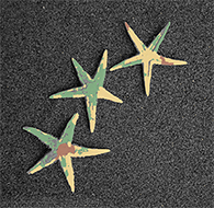
(a) initial seeds	(b) Potts model $\lambda=2$
(c) Potts model $\lambda=6$	(d) Hedgehogs + Potts $\lambda=2$

Figure 9: Three hedgehogs one for each star. (a) shows user scribbles. (c-b) and (d) show Potts model results for different $\lambda$ and our results, respectively. (d) shows that enforcing hedgehogs shape priors (our method) eliminated over-segmented solutions as the one in (b) which is typical for small $\lambda$. (c) shows Potts model result for a larger $\lambda$ at which the stars were not over-segmented, notice star tips were wrongly segmented due to the increase in shrinking bias.

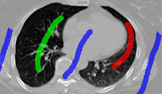
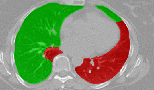
(a) initial seeds	(b) Potts model
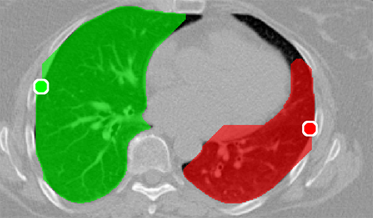
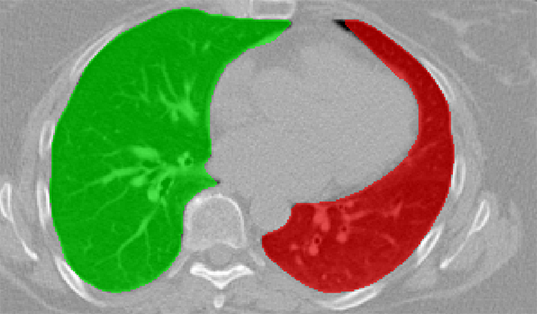
(c) Multi-Star + Potts model	(d) Hedgehogs + Potts model

Figure 10: Two hedgehogs one for each lung. As can be seen in (b) Potts model resulted in segmentation with holes (background inside lungs), and converged to wrong color models. Segmentation holes could be eliminated by using multi-star shape priors (c)—star centers are the midpoints of the green and red circles. However, multi-star can never properly segment the right lung as it is not a star-shape. Our method (Hedgehogs + Potts) (d) eliminated holes and properly segmented the lungs by enforcing a more general shape constraint derived from the user scribble.

In the following set of experiments we show the benefit of incorporating our Hedgehogs term (6) to the well studied Potts model segmentation energy, i.e. data term + smoothness term, for multi-object segmentation in 2D and 3D. We will also give an illustrative real life example to show that the hedgehog shape is more general than star-shape [25]. The results shown in this section for our method were generated using $\theta=\frac{\pi}{4}$ when computing the hedgehog shape constraints, also we did not enforce any shape constraints on the background model. Also, the same smoothness weight $\lambda$ is used when comparing methods unless stated otherwise.

Our optimization framework is similar to [19] where the user marks a set of initial seeds in the form of a scribble for the required labels, e.g. left kidney, right kidney etc. The seeds for each label were used to fit an initial Gaussian Mixture color model, and to generate its hedgehog shape constraints. Similarly to [11, 8], we iteratively optimize our energy (5) (or Potts model) in an EM-style iterative fashion. We alternate between finding a better segmentation and re-estimating the color models using the current segmentation. The framework terminates when it can not decrease the energy anymore.

For the example shown in Fig.9(a), (b-c) show Potts model results for $\lambda=2$ and 6, respectively. It should be noted that $6$ is the smallest smoothness weight that did not result in over-segmentation when using Potts. However, the result in Fig.9(c) is biased towards smaller objects (notice star tips) because by increasing the smoothness weight we are also increasing the shrinking bias. Over-segmented results as the one in Fig.9(b) could be avoided without increasing the shrinking bias, simply by incorporating multi-shape priors. Our method which incorporates Hedgehogs shape priors with Potts model was able to find a better segmentation, see Fig.9(d).

The objective of the example shown in Fig.10(a) is to segment left and right lungs, and the background. Potts model result shown in Fig.10(b) has holes, i.e. part of the background appears in the middle of the lungs. Furthermore, Potts model converged to biased color models where the right lung preferred brighter colors while the left preferred darker colors. Similar to the previous example, increasing $\lambda$ for Potts model will increase the shrinking bias and it becomes hard to segment the elongated part of the the right lung. Using multi-star which is a generalization of [25] to multi-object segmentation is not enough because the right lung is not a star-shape. To be specific, there is no point inside the right lung that could act as a center of a star-shape that would include it. Fig.10(d) shows the result for our method, where user scribbles were used to enforce shape constraints compared to using a single pixel per label [9].

We applied our method on PET-CT scans of three different subjects to segment their liver, left kidney, right kidney and the background. Although we applied our method and Potts model on the 3D volumes we only show the results on a few representative slices from each volume in Fig.11. Also, the results of different methods for each subject were computed using the same smoothness. We can see from the last two rows which compare our method to Potts, using Hedgehogs constraints enabled us to avoid geometrically incorrect segmentations, e.g. one liver inside the other (last-row middle), or parts of left kidney is between the right kidney and liver (last-row right). Furthermore, for test subjects 1 and 2 the kidneys and background were poorly segmented by Potts model, e.g. most of the kidneys were segmented as background for test subject 1. Potts poor performance is due to the large overlap between the kidneys and background color models. This overlap resulted in an in-discriminative data term for Potts to properly separate them. This issue becomes worse in iterative frameworks where color models are re-estimated based on current segmentation. To be specific, if at any iteration Potts model resulted in a bad segmentation then re-estimating the color models will bias them towards the bad segmentation and subsequent iterations worsen the results. Comparing our results for subjects 1 and 2 to Potts model shows that our method is less prone to the aforementioned issue as we forbid undesirable segmentations, i.e. those that do not respect shape constraints.

		Subject 1	Subject 2	Subject 3
	{362.5mm
Our method (Hedgehogs Shapes + Potts)
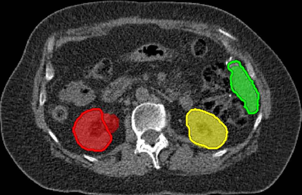
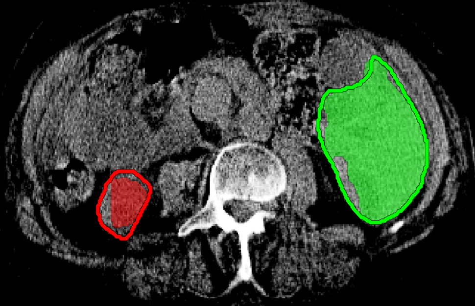
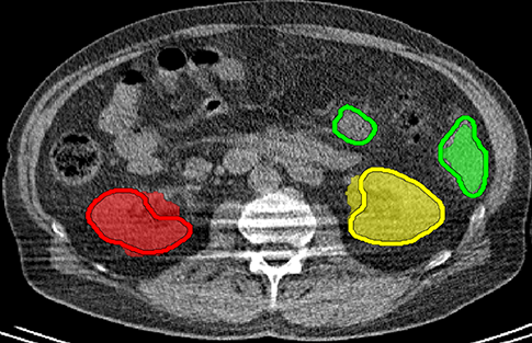
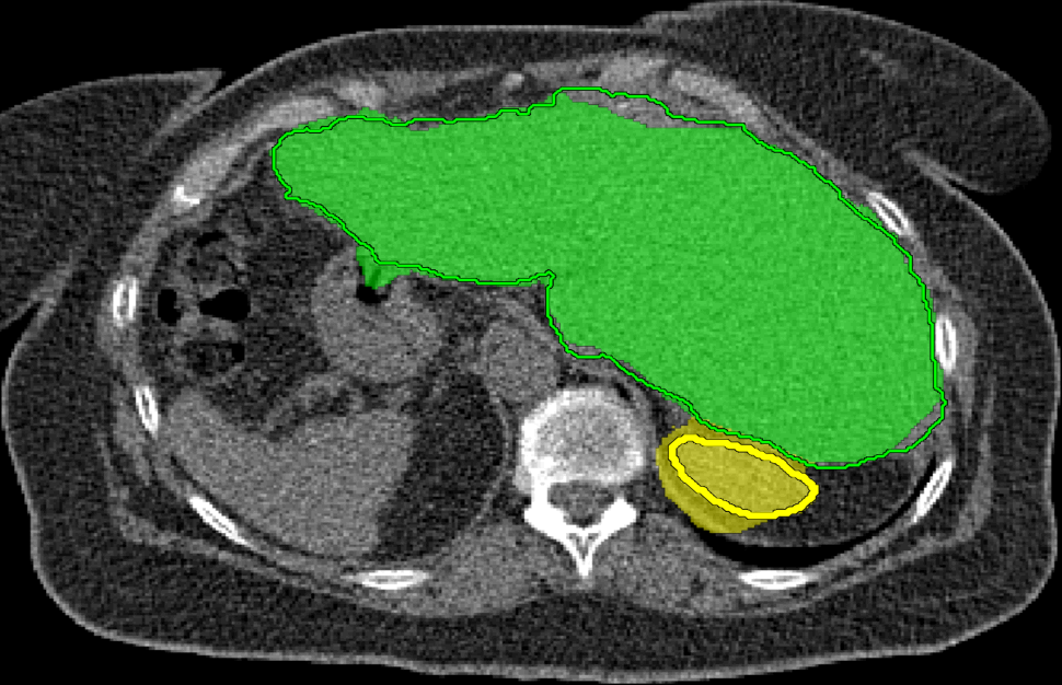
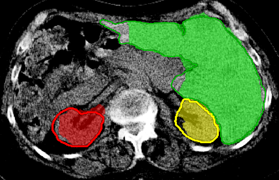
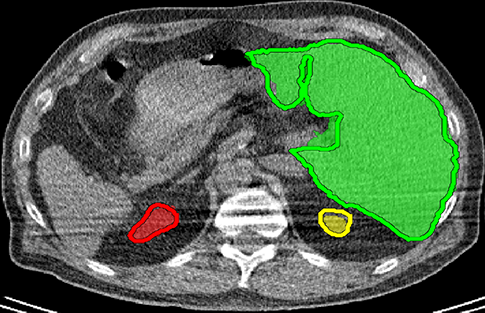
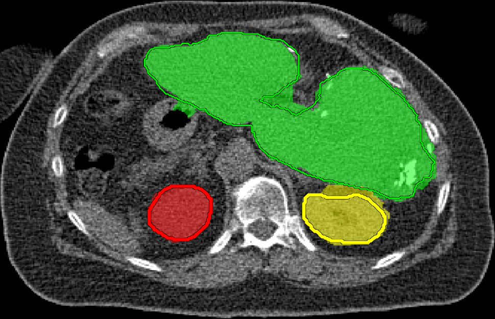
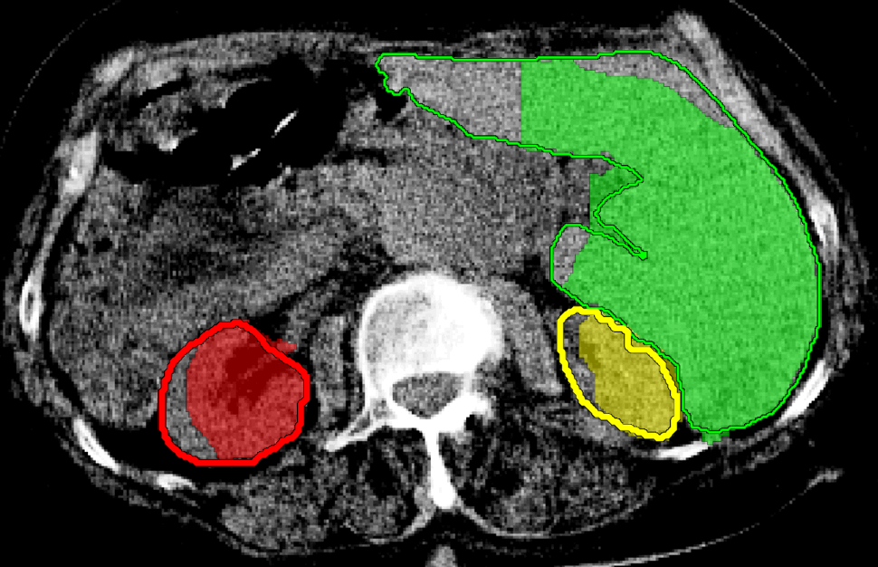
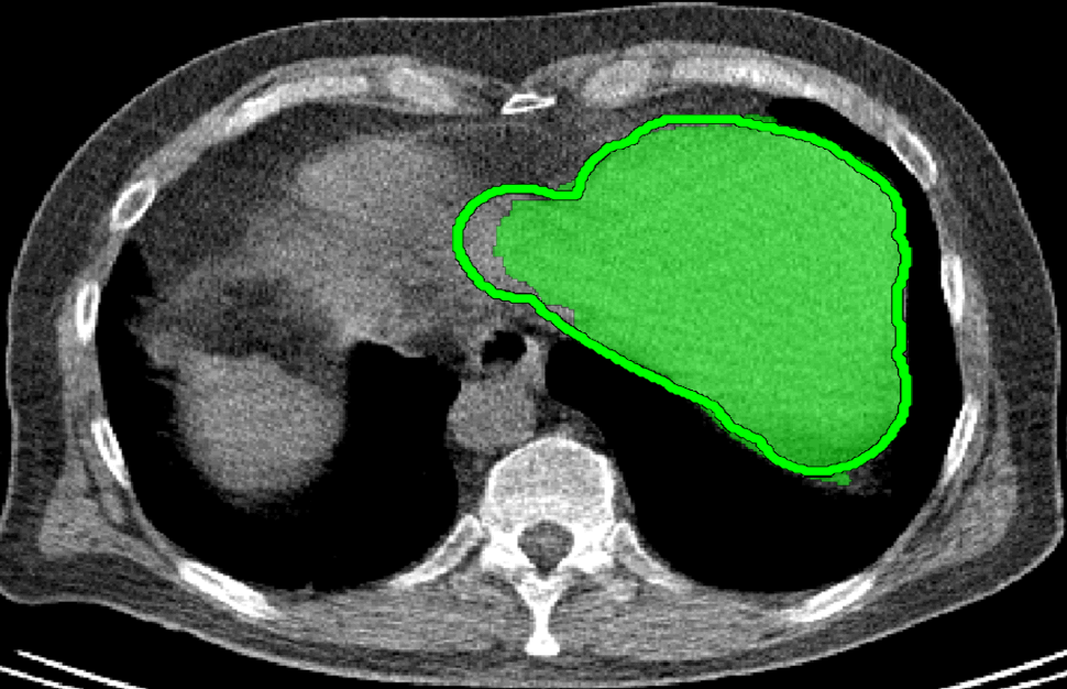
					}1910pt mmmmmmmmmmmSame Slice
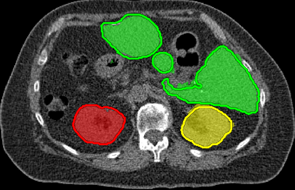
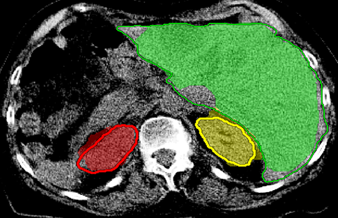
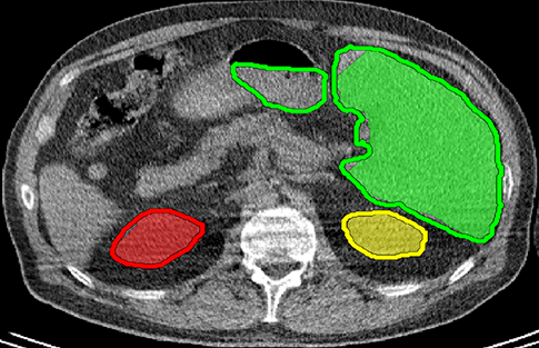
mmmmmPotts

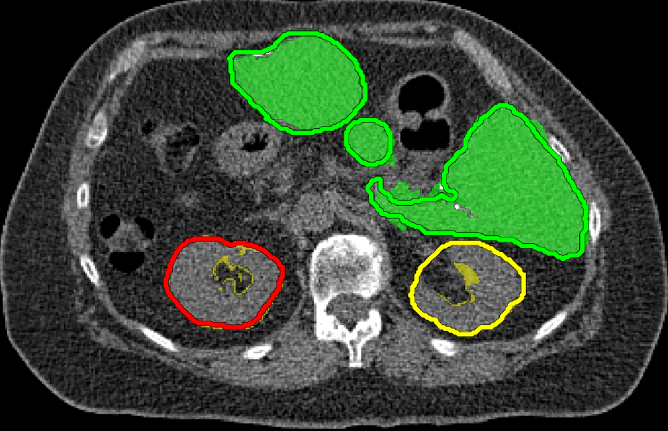
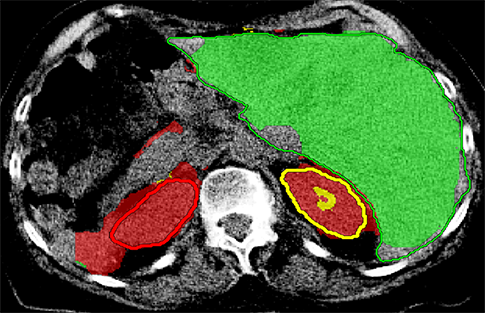
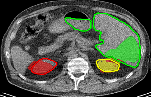
Figure 11: Three hedgehogs for liver and two kidneys, the colored contours represent liver and kidneys ground truth. Each column shows the result of a different test subject. The first four rows show our results, each row represents a different slice. The last row shows Potts model results. Also, the last two rows show results of the same slice for our method and Potts model, respectively. Our method (Hedgehogs+Potts) out performed Potts, results show that enforcing shape constraints avoids/forbids some undesirable segmentations, e.g. for subject 2 Potts segmentation shows that the left kidney surrounds the right kidney, and for subject 3 it shows that part of the left kidney is between the right kidney and liver. In addition, for subjects 1 and 2 Potts model did not properly separate the kidneys from the background.

For quantitative comparison, Table 1 lists for each organ of a subject the $\mathbf{F}_{1}$ Score, Precession and Recall measures of our method and Potts model where $\mathbf{F}_{1}=2*\frac{Precession*Recall}{Precession+Recall}.$ For the kidneys, our method clearly out performed Potts model, e.g. note Potts model poor precision/recall for subjects 1 and 2. For the liver, both methods performed comparably.

	Subject 1		Subject 2		Subject 3
	Ours	Potts	Ours	Potts	Ours	Potts
	Right Kidney
$\mathbf{F}_{1}$ score	$\mathbf{0.85}$	$0.05$	$\mathbf{0.69}$	$0.11$	$\mathbf{0.92}$	$0.85$
Prec.	$0.77$	$0.16$	$0.58$	$0.13$	$0.93$	$0.85$
Recall	$0.96$	$0.03$	$0.84$	$0.10$	$0.91$	$0.87$
	Left Kidney
$\mathbf{F}_{1}$ score	$\mathbf{0.96}$	$0.08$	$\mathbf{0.81}$	$0.48$	$\mathbf{0.93}$	$0.84$
Prec.	$0.90$	$0.97$	$0.85$	0.34	$0.95$	$0.76$
Recall	$0.95$	$0.04$	$0.78$	$0.80$	$0.91$	$0.93$
	Liver
$\mathbf{F}_{1}$ score	$0.92$	$\mathbf{0.93}$	$0.90$	$\mathbf{0.91}$	$\mathbf{0.92}$	$0.84$
Prec.	$0.92$	$0.93$	$0.97$	0.96	$0.97$	$0.96$
Recall	$0.92$	$0.93$	$0.84$	$0.87$	$0.88$	$0.74$

Table 1: The table lists the $\mathbf{F}_{1}$ score, precision and recall measures for each method, individual organ and subject—the closer these values are to 1 the more accurate the segmentation is. For the kidneys where most of the color model overlap occurs, our method was a clear winner. For the liver which has a bigger volume and a more distinct color model compared to the kidneys/background, the two methods performed comparably.

6 Conclusion

We proposed a novel interactive multi-object segmentation method where objects are restricted by hedgehog shapes. The hedgehog shape constraints of an object limits its set of possible segmentations by restricting the segmentation’s allowed surface normal orientations. Hedgehog shape constraints could be derived from some vector field, e.g. the gradient of a user scribble distance transform. In addition, we showed how to modify $\alpha$-expansion moves to optimize our multi-labeling problem with hedgehog constraints. We also proved submodularity of the modified binary expansion moves. Furthermore, we applied our multi-labeling segmentation with hedgehog shapes on 2D images and 3D medical volumes. Our experiments show the significant improvement in segmentation accuracy when using our method over Potts model. Specially in medical data where our method outperformed Potts model in separating multiple organs with similar appearances and weak edges.

Appendix: Discretization Issues

There are some challenges/drawbacks due to the discretization of hedgehog constraints. For example, the number of representable surface orientations depends on the chosen neighborhood system $\mathcal{N}$ which could be remedied by using larger neighborhood systems. Also it is possible for a polar cone ${\hat{C}}_{\theta}(p)$ to be under represented by $\mathcal{E}(\theta)$ if it happens that no edges lie in it which could result in a segmentation surface with folds. Furthermore, in cases where the vector field changes relatively fast w.r.t. the image resolution it is possible for neighboring pixel’s hedgehog constraints to conflict.

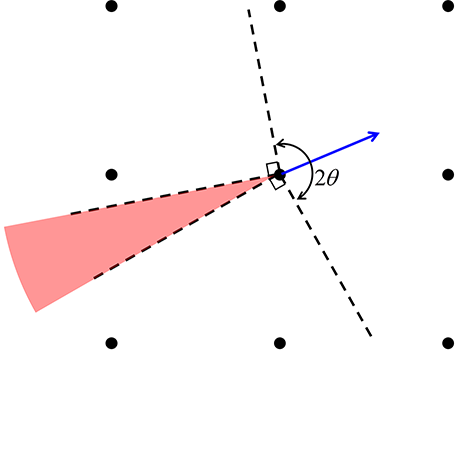
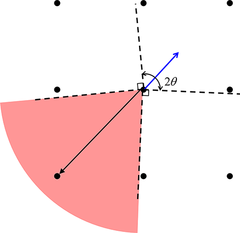
(a) Empty Cone	(b) Under-represented cone
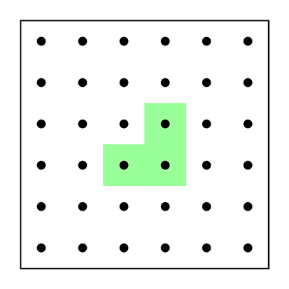
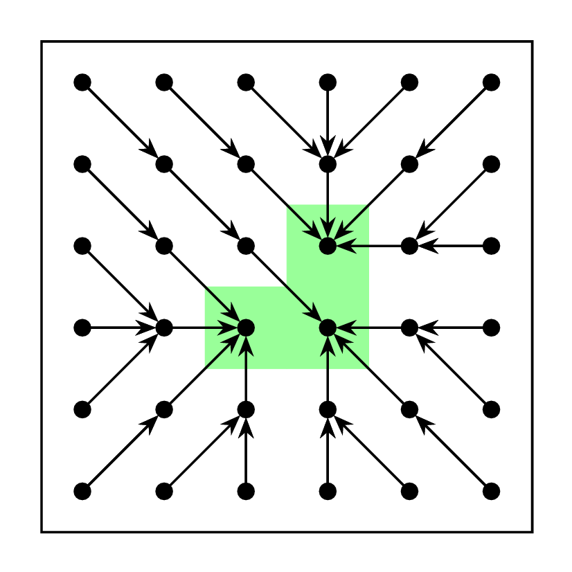
(c) $\mathcal{E}(\frac{\pi}{2})=\phi$	(d) Alternative $\mathcal{E}(\frac{\pi}{2})$

Figure 12: (a-b) illustrate the two cases where a polar cone (shown in red) is under represented by $\mathcal{E}(\theta)$ (shown as black directed edges). (c) shows $\mathcal{E}(\frac{\pi}{2})$ of the surface normals/gradient shown in Fig. 3(a). Note that $\mathcal{E}(\frac{\pi}{2})$ is empty because none of surface normals at any pixel align with its 8-neighbourhood edges. (d) shows the alterative $\mathcal{E}(\frac{\pi}{2})$ where the nearest neighbourhood edge to the empty cone is added as a shape constraint.

Cone under-representation:

a pixel’s polar cone ${\hat{C}}_{\theta}(p)$ is under represented by $\mathcal{E}(\theta)$ in two case: (a) “empty cone ” when there are no neighbor edges consistent with the polar cone as shown in Fig. 12(a), and (b) when there is a large part of the cone unaccounted for, see Fig. 12(b) where the big cone is accounted for by only one edge. Based on our practical experience only ignoring the former case is of significant consequences while ignoring later does not adversary affect the results.

Empty cone issue could be alleviated by increasing the neighborhood size. However, this is not practical because for $\theta=\frac{\pi}{2}$ the neighborhood edge has to perfectly align with the surface normal, see Fig. 12(c). Alternatively, we propose adding to $\mathcal{E}(\theta)$ the nearest neighborhood edge to the empty cone as shown in Fig.12(d).

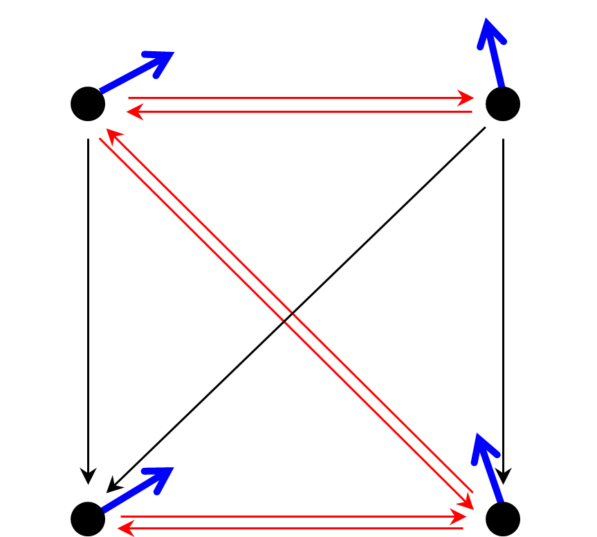
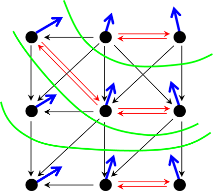
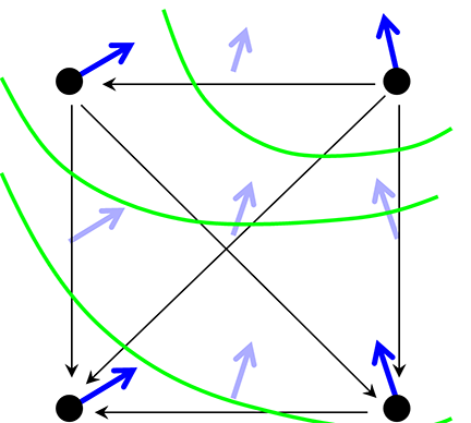
(a) over-constrained $\mathcal{E}(0)$	(b) $\mathcal{E}(0)$ with higher resolution	(c) $\mathcal{E}(0)$ after edge pruning

Figure 13: Permissible segmentations shown in green, $\mathcal{E}(0)$ shown in black and red, and vector field shown in blue. (a) shows $\mathcal{E}(0)$ where over-constraining occurs due to the rapid change in orientation. (b) shows how increasing the solution could solve the over-constraining issue. (c) shows the case where edges in $\mathcal{E}(0)$ were eliminated when they were inconsistent with the interpolated vector field (shown in light blue).

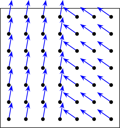
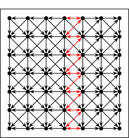
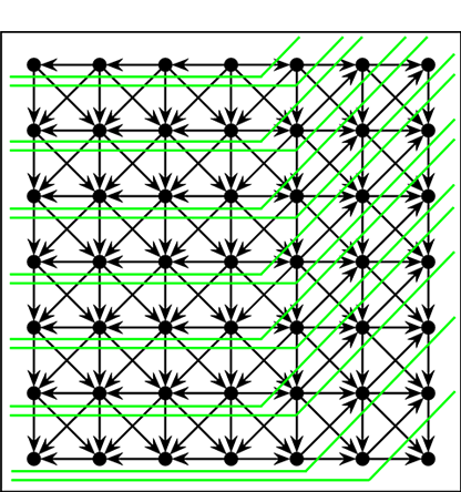
(a) vector field with rapid changes	(b) $\mathcal{E}(0)$	(c) $\mathcal{E}(0)$ after pruning

Figure 14: (a) vector field. (b) $\mathcal{E}(0)$ of (a) where over-constraining occurs (shown in red). In (b) only the trivial segmentations are allowed due to over-constraining. (c) shows $\mathcal{E}(0)$ after pruning and the non-trivial segmentations (shown in green) allowed by that construction.

Fast changing vector field:

hedgehog prior (3) enforces the shape constraints at every pixel independently. When the vector field orientation changes rapidly between neighboring pixels the resulting shape constraints could become contradictory leading to over-constraining. As can be seen in Fig. 13(a) the contradictory shape constraints resulted in a construction where no surface could path between the four neighboring pixels, i.e. all of them will either be labeled foreground or background.

One possible way to overcome the fast changing vector fields is to increase the image resolution via sub-sampling. As you can see in Fig. 13(b) doubling the resolution alleviated the aforementioned issue. However, there is no simple answer to at which resolution there will be no over-constraining, as it will depend on $\theta$, $\mathcal{N}$ and the vector field. Also, increasing the image resolution is not a practical solution as it adversely affects the running time.

Alternatively one can try an resolve contradicting constraints by pruning $\mathcal{E}(\theta)$. In this case, we interpolate the vector field’s orientation for every neighboring pixels and eliminate their edge constraint(s) if it were not consistent with the interpolated orientation, as shown in Fig. 13(c). Fig14 shows a synthetic example of fast chancing vector field orientations and how the edge constraints pruning alleviates the over-constraining problem.

References

- [1] S. Andrews, C. McIntosh, and G. Hamarneh. Convex multi-region probabilistic segmentation with shape prior in the isometric log-ratio transformation space. In Computer Vision (ICCV), 2011 IEEE International Conference on, pages 2096–2103. IEEE, 2011.
- [2] Y. Boykov and M.-P. Jolly. Interactive graph cuts for optimal boundary & region segmentation of objects in N-D images. In ICCV, volume I, pages 105–112, July 2001.
- [3] Y. Boykov and V. Kolmogorov. Computing geodesics and minimal surfaces via graph cuts. In International Conference on Computer Vision, volume I, pages 26–33, 2003.
- [4] Y. Boykov, O. Veksler, and R. Zabih. Fast approximate energy minimization via graph cuts. In International Conference on Computer Vision, volume I, pages 377–384, 1999.
- [5] Y. Boykov, O. Veksler, and R. Zabih. Fast approximate energy minimization via graph cuts. IEEE transactions on Pattern Analysis and Machine Intelligence, 23(11):1222–1239, November 2001.
- [6] D. Cremers, F. R. Schmidt, and F. Barthel. Shape priors in variational image segmentation: Convexity, lipschitz continuity and globally optimal solutions. In Computer Vision and Pattern Recognition, 2008. CVPR 2008. IEEE Conference on, pages 1–6. IEEE, 2008.
- [7] A. Delong and Y. Boykov. Globally Optimal Segmentation of Multi-Region Objects. In International Conference on Computer Vision (ICCV), 2009.
- [8] A. Delong, A. Osokin, H. Isack, and Y. Boykov. Fast Approximate Energy Minization with Label Costs. International Journal of Computer Vision (IJCV), 96(1):1–27, January 2012.
- [9] P. F. Felzenszwalb and O. Veksler. Tiered scene labeling with dynamic programming. In Computer Vision and Pattern Recognition (CVPR), 2010.
- [10] V. Gulshan, C. Rother, A. Criminisi, A. Blake, and A. Zisserman. Geodesic star convexity for interactive image segmentation. In Proceedings of the IEEE Conference on Computer Vision and Pattern Recognition, 2010.
- [11] H. N. Isack and Y. Boykov. Energy-based Geometric Multi-Model Fitting. International Journal of Computer Vision (IJCV), 97(2):123–147, April 2012.
- [12] H. Ishikawa. Exact optimization for Markov Random Fields with convex priors. IEEE transactions on Pattern Analysis and Machine Intelligence, 25(10):1333–1336, 2003.
- [13] J. Kappes, B. Andres, F. Hamprecht, C. Schnorr, S. Nowozin, D. Batra, S. Kim, B. Kausler, J. Lellmann, N. Komodakis, et al. A comparative study of modern inference techniques for discrete energy minimization problems. In Computer Vision and Pattern Recognition (CVPR), pages 1328–1335, 2013.
- [14] V. Kolmogorov and Y. Boykov. What metrics can be approximated by geo-cuts, or global optimization of length/area and flux. In International Conference on Computer Vision, October 2005.
- [15] V. Kolmogorov and R. Zabih. What energy functions can be minimized via graph cuts. In 7th European Conference on Computer Vision, volume III of LNCS 2352, pages 65–81, Copenhagen, Denmark, May 2002. Springer-Verlag.
- [16] K. Li, X. Wu, D. Z. Chen, and M. Sonka. Optimal surface segmentation in volumetric images-a graph-theoretic approach. IEEE transactions on Pattern Analysis and Pattern Recognition (PAMI), 28(1):119–134, January 2006.
- [17] S. M. Pizer, P. T. Fletcher, S. Joshi, A. Thall, J. Z. Chen, Y. Fridman, D. S. Fritsch, A. G. Gash, J. M. Glotzer, M. R. Jiroutek, et al. Deformable m-reps for 3d medical image segmentation. International Journal of Computer Vision, 55(2-3):85–106, 2003.
- [18] S. Pizer et al. Deformable M-Reps for 3D Medical Image Segmentation. International Journal of Computer Vision (IJCV), 55(2-3):85–106, November 2003.
- [19] C. Rother, V. Kolmogorov, and A. Blake. Grabcut - interactive foreground extraction using iterated graph cuts. In ACM transactions on Graphics (SIGGRAPH), August 2004.
- [20] C. Rother, V. Kolmogorov, V. Lempitsky, and M. Szummer. Optimizing binary mrfs via extended roof duality. In Computer Vision and Pattern Recognition (CVPR), pages 1–8, 2007.
- [21] F. Schmidt and Y. Boykov. Hausdorff distance constraint for multi-surface segmentation. In European Conference on Computer Vision (ECCV), LNCS 7572, volume 1, pages 598–611, Florence, Italy, October 2012.
- [22] T. Schoenemann and V. Kolmogorov. Generalized sequential tree-reweighted message passing. Advanced Structured Prediction, page 75, 2014.
- [23] K. Siddiqi and S. Pizer. Medial representations: mathematics, algorithms and applications, volume 37. Springer Science & Business Media, 2008.
- [24] K. Siddiqi and S. Pizer. Medial Representations: Mathematics, Algorithms and Applications. Springer, December 2008.
- [25] O. Veksler. Star shape prior for graph-cut image segmentation. In European Conference on Computer Vision (ECCV), 2008.
- [26] N. Vu and B. Manjunath. Shape prior segmentation of multiple objects with graph cuts. In Computer Vision and Pattern Recognition (CVPR), pages 1–8, 2008.