Spontaneous symmetry breaking of self-trapped and leaky modes in quasi-double-well potentials

Abstract

We investigate competition between two phase transitions of the second kind induced by the self-attractive nonlinearity, viz., self-trapping of the leaky modes, and spontaneous symmetry breaking (SSB) of both fully trapped and leaky states. We use a one-dimensional mean-field model, which combines the cubic nonlinearity and a double-well-potential (DWP) structure with an elevated floor, which supports leaky modes (quasi-bound states) in the linear limit. The setting can be implemented in nonlinear optics and BEC. The order in which the SSB and self-trapping transitions take place with the growth of the nonlinearity strength depends on the height of the central barrier of the DWP: the SSB happens first if the barrier is relatively high, while self-trapping comes first if the barrier is lower. The SSB of the leaky modes is characterized by specific asymmetry of their radiation tails, which, in addition, feature a resonant dependence on the relation between the total size of the system and radiation wavelength. As a result of the SSB, the instability of symmetric modes initiates spontaneous Josephson oscillations. Collisions of freely moving solitons with the DWP structure admit trapping of an incident soliton into a state of persistent shuttle motion, due to emission of radiation. The study is carried out numerically, and basic results are explained by means of analytical considerations.

I Introduction

Usually, the ground state (GS) of quantum-mechanical systems exactly follows the symmetry of the underlying Hamiltonian LL , while excited states may realize different representations of the same symmetry (a different situation is exemplified by the Jahn-Teller effect in molecules, which makes the GS of the electron subsystem spatially asymmetric, thus breaking the symmetry of the respective Hamiltonian RE ). In particular, for the double-well potential (DWP), which is dealt with in the present work, the GS wave function is spatially even, while the first excited state is odd. This is not necessarily true in many-body settings. In that context, the mean-field description of atomic Bose-Einstein condensates (BECs) is provided by the Gross-Pitaevskii equation (GPE) BEC , which includes the cubic term accounting for attractive forces between colliding atoms. Essentially the same is the nonlinear Schrödinger equation (NLSE) modeling the propagation of optical signals in Kerr-nonlinear media NLS . If the self-focusing nonlinearity is strong enough, it gives rise to the phase transition in the form of spontaneous symmetry breaking (SSB) of the GS book . In its simplest manifestation, which is provided by the DWP, the SSB implies that one well traps a larger atomic density or field power than the other. This effect also implies the breakup of the basic principle of quantum mechanics, according to which the GS cannot be degenerate, as the SSB gives rise to a pair of two mutually symmetric GSs in the DWP, with the maximum of the wave function found in either potential well (as mentioned above, the Jahn-Teller effect gives rise to a qualitatively similar situation). The same DWP setting admits a symmetric state coexisting with the asymmetric ones, but, above the SSB point, the symmetric wave function no longer represents the GS, being unstable against symmetry-breaking perturbations. In the course of the spontaneous transition from the unstable symmetric state to a stable asymmetric one, the choice between the two mutually degenerate asymmetric states is determined by random perturbations, which push the system to build the maximum of the wave function in the left or right potential well. The SSB is a ubiquitous phenomenon, with well-known manifestations in nonlinear optics, BEC, superfluidity, superconductivity, ferromagnetism, etc. book .

The concept of the SSB in nonlinear systems of the NLS type was, plausibly, introduced for the first time in 1979 by E. B. Davies Davies , who addressed a nonlinear extension of the Schrödinger equation for a pair of quantum particles with an isotropic interaction potential. In this context, the SSB was predicted as the breaking of the rotational symmetry in the GS. Another early work, which predicted the SSB in a relatively simple form, addressed the self-trapping model, based on a system of linearly coupled ordinary differential equations including the self-attractive cubic terms Scott .

In the effectively one-dimensional geometry, the SSB can be studied in the framework of the scaled NLSE/GPE with potential $H(x)$ of the DWP type, for the amplitude of the electromagnetic wave, or the single-particle wave function, $\psi\left(x,z\right)$:

$$i\frac{\partial\psi}{\partial z}=-\frac{1}{2}\frac{\partial^{2}\psi}{\partial x^{2}}-\left|\psi\right|^{2}\psi+H(x)\psi,$$ (1)

where $z$ is the propagation distance in optics, or time in the GPE. This equation can be reduced to a system of coupled ordinary differential equations for two amplitudes, $u_{1,2}(z)$, by means of the tight-binding approximation tight , which replaces $\psi(x,z)$ by a linear superposition of two stationary wave functions, $\phi$, corresponding to the states trapped separately in either potential well, with their centers located at $x=\pm a$ Ananikian :

$$\psi\left(x,z\right)=u_{1}(z)\phi\left(x-a\right)+u_{2}(z)\phi\left(x+a\right).$$ (2)

The analysis of the SSB in BEC and similar models based on Eq. (1) was initiated in Refs. Milburn and Smerzi . In this case, in the framework of the mean-field approximation, the symmetry breaking is the phase transition of the second kind (alias the supercritical bifurcation, which does not admit hysteresis Joseph ). Further, GPE (1) was extended by adding an extra (free) spatial coordinate, which transforms the DWP into a two-dimensional dual-core structure Warsaw . In such a setting, the self-attractive nonlinearity gives rise to matter-wave solitons, which self-trap in the free direction soliton . The SSB destabilizes symmetric solitons and replaces them by asymmetric ones, provided that the norm of the wave function (which determines the effective strength of the intrinsic nonlinearity) exceeds a critical value Warsaw . In the latter case, the mean-field symmetry breaking is a phase transition of the first kind (alias a subcritical bifurcation Joseph ), which includes hysteresis. The subcritical transition is typical to solitons in dual-core waveguides with the Kerr self-focusing soliton-dual-core . The same type of the transition may be featured by CW (continuous-wave) states in dual-core systems with non-Kerr nonlinearities Snyder .

In addition to the analysis of static symmetric and asymmetric modes, dynamical regimes, most typically in the form of oscillations of the mean-field wave function between two wells of the DWP structure, were analyzed too. Following the analogy with Josephson oscillations of the wave function of Cooper-paired electrons in superconducting tunnel junctions Ustinov , the possibility of oscillations in bosonic Josephson junctions was predicted junction . The simplest dynamical model of the Josephson oscillations in bosonic systems was derived by means of the tight-binding approximation (superconductor ).

Experimental manifestations of the SSB have been observed in both BEC and photonics. Self-trapping of a macroscopically asymmetric state of the atomic condensate of ⁸⁷Rb atoms, loaded into the DWP, as well as Josephson oscillations in that setting, were reported in Ref. Markus (in that case, the effective nonlinearity is self-repulsive, therefore the respective SSB occurs not in the symmetric GS, but rather in the antisymmetric first excited state). The SSB of laser beams coupled into an effective transverse DWP created in the self-focusing photorefractive medium was demonstrated in Ref. photo . Other experimentally observed SSB effects in optics are spontaneously established asymmetric regimes of operation of coupled lasers lasers ; NatPhot ; NaturePhot2 ; Chili , and breaking of chiral symmetry in metamaterials Kivshar .

In addition to usual bound states, one may work with quasi-localized modes in potentials which do not admit complete trapping in linear quantum mechanics, but give rise to leaky bound states, alias quasi-bound ones. The combination of such a potential and self-attractive nonlinearity makes it possible to transform the leaky states into truly bound ones Carr1 ; Carr2 . This possibility, in turn, suggests another setting, which is the subject of the present work: DWP structures embedded into a potential barrier. In the linear limit, this structure support solely symmetric leaky modes, that may be transformed into self-trapped ones with the help of the cubic self-attraction. The main feature of the system which, to the best of our knowledge, was not explored before, is competition between two different mean-field phase transitions of the second kind, driven by the nonlinearity: the SSB and transition to the self-trapping. Realization of the competition in stationary states of the DWP system is the main subject of the present work. We demonstrate that, depending on parameters of the DWP structure and nonlinearity strength, either transition may happen first, with the growth of the nonlinearity. Another essential problem addressed in the paper is a dynamical one, namely, Josephson oscillations in the DWP structure, initiated by the instability of the symmetric mode, and collisions of free solitons with the structure.

It is relevant to mention that, in terms of the BEC realizations, the present setting represents macroscopic quantum states, with the phase transitions between them being quasi-classical ones, considered in the framework of the mean-field approximation. The validity of this approximation is usually justified by the large number of atoms in the condensate BEC . The consideration of a few-body state in the DWP can give rise to quantum phase transitions, such as those in the Lipkin-Meshkov-Glick model, which applies in this case LMG . As suggested by a recent analysis of the three-dimensional many-body quantum gas with repulsive binary interactions, which is pulled to the center by a potential $\sim-1/r^{2}$ Grisha , the quantum phase transition may produce results similar to but different from their mean-field counterparts HS . In particular, the GS predicted by the mean-field may be replaced by a metastable state in the quantum many-body theory Grisha . In any case, the consideration of truly quantum phase transitions in the DWP structure is a subject for a separate work.

The subsequent presentation is structured as follows. The model is elaborated in Section II. Results of the analysis of symmetric and spontaneously emerging asymmetric trapped and leaky modes in it are summarized in Section III. Detailed results are obtained in a numerical form, and their basic features are explained by means of an analytical approach. Both the trapped and leaky modes undergo the SSB transition with the increase of the norm, the symmetric modes getting unstable above the transition point. The nonlinear evolution of the unstable modes, which features Josephson oscillations, is studied by means of systematic simulations in Section IV. A related possibility is capture of incident solitons by the DWP structure into shuttle states. This possibility is studied in a systematic form in Section V. The paper is concluded by Section VI.

II The model

The underlying dynamical model, based on Eq. (1), gives rise to stationary modes with propagation constant $k$ (in BEC, $-k$ is the chemical potential),

$$\psi\left(x,z\right)=e^{ikz}u\left(x\right),$$ (3)

where real modal functions $u(x)$ satisfy the equation

$$-ku+\frac{1}{2}u^{\prime\prime}+u^{3}=H\left(x\right)u.$$ (4)

Solutions with $k>0$ represent self-trapped localized states, while $k<0$ corresponds to delocalized leaky modes, which do not vanish at $x\rightarrow\pm\infty$. The states of these two types are characterized, respectively, by convergent and divergent norms, $N=\int_{-\infty}^{+\infty}u^{2}(x)dx$ (proportional to the total power of the light beam in optics, or the total number of atoms in BEC), and Hamiltonian (energy),

$$E=\int_{-\infty}^{+\infty}\left[\frac{1}{2}\left(u^{\prime}\right)^{2}-\frac{1}{2}u^{4}+2H(x)u^{2}\right]dx.$$ (5)

The DWP can be readily implemented in the experiment. In optics, waveguides with this structure are fabricated with the help of the implanting technique Opt-DWP , while in BEC the DWP setting can be created by means of electromagnetic fields BEC-DWP . In the present work, calculations are reported for the rectangular DWP profile with the elevated floor:

$$H\left(x\right)=\left\{\begin{array}[]{ll}A,&~{}\mathrm{at}~{}~{}|x|<0.5,\\ 2,&~{}\mathrm{at}~{}~{}3<|x|<7,\\ 0,&~{}\mathrm{elsewhere},\end{array}\right.$$ (6)

where $A>0$ is the height of the inner potential barrier, see Fig. 1, while height $H_{\max}=2$ of the outer barriers is fixed by scaling. Values of lengths adopted in Eq. (6) adequately represent the generic situation, as demonstrated by additional numerical results (not shown here in detail). Indeed, it is shown below that the symmetry-breaking and self-trapping transitions, and the competition between them, crucially depend on the tunneling transparency of the central barrier and the nonlinearity strength, i.e., the barrier height, $A$, and total norm, $N$. These are two control parameters which are subject to the variation in the subsequent analysis. For the same reason, the main findings are not sensitive to a particular shape of the DWP. In particular, the rectangular form of the DWP, adopted in Eq. (6), which may be essential for some dynamical effects, such as temporal scaling in the relaxation of perturbations Azbel , produces results which are essentially the same as generated by smooth DWP profiles (for the self-trapping of the leaky modes in a single potential well, this property was known before Carr1 ). As concerns the necessity of having the elevated potential floor, it may make the experimental creation of the structure easier, as the “floor” is naturally built by overlap of fringes of two potential barriers which determine the DWP (in previously reported experimental realizations of the DWP in BEC Markus , the bottom level of the potential had to be depressed, because those DWPs trapped condensates with the repulsive interactions, on the contrary to the case of the self-attraction, considered herein).

Figure 1: The symmetric double-well potential for leaky modes (quasi-bound states), defined as per Eq. (6).

Obviously, in the absence of the self-attractive cubic term, potential (6) cannot support any bound state in the respective linear model, while weakly delocalized quasi-bound states are possible. Indeed, a straightforward estimate of the tunneling coefficient for the tall barriers separating the inner and outer parts of structure (6) yields

$$T\simeq\exp\left(-\sqrt{2H_{\max}-q^{2}}W\right)\approx\allowbreak 4.4\times 10^{-4},$$ (7)

where $H_{\max}=2$ and $W=4$ are the height and width of the potential barriers, as per Eq. (6), and $q\equiv\pi/l=\pi/6$ is the wavenumber of the lowest quasi-bound state in the potential box of width $l=6$.

For the study of collisions of moving solitons with the DWP structure, the height of the inner barrier is fixed to be $A=0.5$, while the height, $H_{0}$, and width, $W_{0}$, of the outer barriers will be varied, to allow clearer observations of different collision scenarios:

$$H\left(x\right)=\left\{\begin{array}[]{ll}0.5,&~{}\mathrm{at}~{}~{}|x|<0.5,\\ H_{0},&~{}\mathrm{at}~{}~{}3<|x|<3+W_{0}\equiv\Lambda/2,\\ 0,&~{}\mathrm{elsewhere}.\end{array}\right.$$ (8)

Detailed consideration of the SSB in the leaky modes will require an explicit calculation of small-amplitude radiation tails attached to those modes outside of the barriers, i.e., at $|x|>7$, see Eq. (6). For this purpose, the DWP is embedded into a broad free-space domain, $|x|<L/2$, with zero boundary conditions (b.c.):

$$u(|x|=L/2)=0.$$ (9)

III Spontaneous symmetry breaking (SSB) of leaky and trapped modes

III.1 The structure of symmetric and asymmetric modes

Numerical solutions of Eq. (4) were obtained by means of the shooting and Newton-matrix methods. While the former one makes it possible to find all relevant solutions independently of an input trial function, the latter method can be applied to obtain solution with high accuracy, provided that the initial guess is taken not too far from the final result. For the setting addressed in this paper, the combination of both algorithms is the most efficient way of obtaining stationary solutions.

As is typical for the SSB in systems with self-focusing nonlinearity, it was found that the GS is spatially symmetric below the bifurcation point ($k<k_{\mathrm{bif}}$) and asymmetric above it, at $k>k_{\mathrm{bif}}$. The symmetric state exists at $k>k_{\mathrm{bif}}$ too, but in that case it is not a GS, and is no longer stable. As mentioned above, all mean-field phase transitions exhibited by the present system are of the second kind, featuring no hysteresis or bistability between symmetric and asymmetric modes.

Generic examples of unstable symmetric and stable asymmetric states of both trapped ($k>0$) the leaky ($k_{\mathrm{bif}}<k<0$) types are displayed in Figs. 2(a) and (b), respectively. In the latter case, the delocalized tails of the leaky mode are extremely small, with amplitude

$$u_{\mathrm{rad}}^{(\max)}\approx 1.2\times 10^{-4}.$$ (10)

Taking into regard the value of the amplitude of the delocalized mode at its center, $U_{0}\approx 0.40$, tunneling coefficient (7) predicts amplitude $u_{\mathrm{rad}}^{(\max)}\sim TU_{0}\simeq 1.8\times 10^{-4}$, in reasonable agreement with its numerically found counterpart (10). For given $k$, the spatial period of the tail in the free space is expected to be $\lambda=\pi\sqrt{2/|k|}\approx\allowbreak 15$ for $k=-0.085$ in Fig. 2(b), while the numerical solutions demonstrates a close value, $\lambda\approx 13.5$ (a small deviation from the predicted value may be explained by the proximity of the tail to the outer barrier).

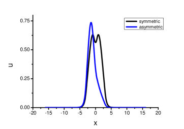
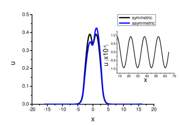
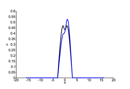
Figure 2: (Color online) (a) Typical examples of trapped symmetric (black) and asymmetric (blue, gray in printed version) states for propagation constant $k=0.1$, the respective norms being $N_{\mathrm{symm}}=1.542$ and $N_{\mathrm{asym}}=1.082$. (b) The same for leaky modes, at $k=-0.085$, with $N_{\mathrm{symm}}=0.642$ and $N_{\mathrm{asym}}=0.630$. The inset in (b) zooms in on one spatial period the small oscillatory tail of the symmetric leaky mode. For the sake of comparison, panel (c) displays the symmetric and asymmetric states with the same $k$ as in (b), but trapped in DWP (6) with impenetrable outer barriers (i.e., $H=2$ is replaced by $H=\infty$ in them), the respective norms being $N_{\mathrm{symm}}=0.792$ and $N_{\mathrm{asym}}=0.769$. All the modes are produced by potential (6) with the height of the inner barrier $A=0.5$.

The formally diverging contribution of the tails to the total norm of the leaky mode is negligible, $N_{\mathrm{rad}}\simeq\left(L/2\right)\left[u_{\mathrm{rad}}^{(\max)}\right]^{2}$, where $L\approx 20$ is the total size of the free-space part of the configuration displayed in Fig. 2(b). Indeed, using estimate (10) for the tail’s amplitude yields $N_{\mathrm{rad}}\sim 10^{-7}$, therefore the leaky modes have definite values of the norm, as indicated in the caption to Fig. 2(b).

For the sake of direct comparison between leaky and trapped modes, in Fig. 2(c) we display stationary states with the same propagation constant as in Fig. 2(b), but in the case when they are confined by impenetrable (infinitely tall) outer potential barriers in Eq. (6). It is seen that, similar to the situation shown in Fig. 2(b), the smaller and larger values of $N$ correspond to the broken asymmetric and unbroken symmetric modes, respectively. However, in the infinitely deep potential box the profiles of the wave functions are, naturally, narrower and taller.

The symmetric modes displayed in Fig. 2 feature split peaks, due to the fact that the inner potential barrier in Eq. (6) is relatively high. On the other hand, the same potential structure with an essentially smaller barrier’s height $A$ supports single-peak symmetric modes, see Fig. 6 below.

III.2 SSB of radiation tails in leaky modes

As mentioned above, the SSB of trapped modes is a known effect, which was previously studied in other forms book ; NaturePhot2 . A new phenomenon reported here is the SSB of leaky modes, which include nonvanishing tails extending into the free space outside of the DWP structure. Even if the tails have small amplitudes, it is interesting to analyze their structure in asymmetric modes, as this issue was not considered previously. To this end, we here focus on the symmetric and asymmetric states in the setting based on the DWP (6) with $A=0.5$ and $\Lambda=14$, embedded into a broad domain of size $L=128$, see Eqs. (6), (8), and (9). In this case, the asymmetric modes are found at $k\geq-0.100$.

A characteristic example of asymmetric tails, i.e., left and right ones with unequal amplitudes, is shown in Fig. 3(a) for $k=-0.075$. Further, separately calculated total norms of the right and left tails, in regions $\Lambda/2<x<L/2$ and $-\Lambda/2<x<-L/2$, along with the norm of the tails in the coexisting unstable symmetric leaky mode, are displayed, as functions of $k$, in Fig. 3(b). This dependence exhibits two notable features. First, the asymmetry between the right and left tails emerges at $k=-0.100$ and gradually increases with the increase of $k$ (i.e., decrease of $|k|$), even if each tail’s norm vanishes in the limit of $k$$\rightarrow 0$ (when the transition to the self-trapped mode takes place, and the tails vanish). This feature is illustrated by Fig. 3(c), which displays the asymmetry measure vs. $k$:

$$\theta(k)\equiv\frac{\int_{\Lambda/2}^{L/2}u^{2}(x;k)dx-\int_{-\Lambda/2}^{-L/2}u^{2}(x;k)dx}{\int_{\Lambda/2}^{L/2}u^{2}(x;k)dx+\int_{-\Lambda/2}^{-L/2}u^{2}(x;k)dx}~{}.$$ (11)

Second, the dependence of the tails’ norms on $k$ shows strong oscillations, which is explained by the commensurability-incommensurability transitions between the wavelength of the radiation tail and the total size of the free-space domains, $L/2-\Lambda/2$. Indeed, the radiation wavenumber given by the free-space dispersion relation for linearized equation (4), $q=\sqrt{-2k}$, determines the the radiation half-wavelength, $\pi/q$, which, in the case of the commensurability, satisfies relation $(\pi/q)n=L/2-\Lambda/2$, with $n=1,2,3,...$ . Thus, maxima of the radiation amplitude are expected at discrete values of the propagation constant,

$$k_{n}=-2\left[\pi n/\left(L-\Lambda\right)\right]^{2}.$$ (12)

As shown in Fig. 3(b), Eq. (12) quite accurately predicts positions of the tail-norm peaks for $n=2,3,4,5,6,7,$ and $8$, for $L-\Lambda=114$, which corresponds to the present case [$n=1$ yields $k_{1}\approx-1.5\times 10^{-3}$, for which the tail’s amplitudes are too small to discern the corresponding maximum, while Eq. (12) with $n=9$ predicts $k_{9}\approx-0.123$, for which asymmetric modes do not exist).

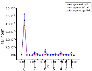
Figure 3: (Color online) (a) A typical example of tails of an asymmetric leaky mode, found at propagation constant $k=-0.075$. (b) The total norms of the right and left tails of the asymmetric leaky mode, along with the tail norm for its symmetric counterpart, vs. $k$. Vertical arrows indicate positions of the maxima predicted, through the commensurability condition, by Eq. (12). (c). The asymmetry parameter for the tails’ norm, defined as per Eq. (11), vs. $k$. These results were obtained for $A=0.5$ in DWP structure (6), and the total size of the system $L=128$.

III.3 SSB diagrams

Getting back to the consideration of the SSB for the entire system, systematic results are presented by means of plots $N(k)$ and $E(N)$ [the Hamiltonian is defined by Eq. (5)] for symmetric and asymmetric modes, which are displayed in Figs. 4(a-c) and (d-f) for three different values of height $A$ of the inner barrier of potential structure (6). Note that the $N(k)$ curves obey the Vakhitov-Kolokolov criterion VK ; VK2 , which is necessary but not sufficient for the stability of modes supported by the self-attractive nonlinearity (it does not catch the instability of the symmetric modes coexisting with asymmetric ones). It is relevant to compare these plots with their counterparts,

$$N_{\mathrm{sol}}=2\sqrt{2k},~{}E_{\mathrm{sol}}=-(1/3)\left(2k\right)^{3/2}\text{,}$$ (13)

for the NLS solitons in the free space, given by Eq. (3) with

$$u_{\mathrm{sol}}(x)=\sqrt{2k}\,\mathrm{sech}\left(\sqrt{2k}x\right),$$ (14)

which are displayed by dashed curves in Figs. 4(a-f).

The SSB in the families of trapped and leaky states is characterized by the asymmetry ratio,

$$\Theta\equiv N^{-1}\left[\int_{0}^{+\infty}u^{2}(x)dx-\int_{-\infty}^{0}u^{2}(x)dx\right]$$ (15)

[cf. a similar definition for the tails, given by Eq. (11)], which is shown as a function of $N$ in Figs. 4(g-i). These plots clearly identify the SSB-onset points, at which the symmetric mode gets destabilized, and simultaneously a stable asymmetric one emerges. In accordance with what is said above, the bifurcation is of the supercritical type Joseph , i.e., the emerging branches of the asymmetric states immediately go “forward”. Conclusions about the stability and instability of the solution branches displayed in Fig. 4 were produced by means of the well-known method VK2 based on numerical computation of (in)stability eigenvalues (imaginary parts of eigenfrequencies) for small perturbations added to the stationary solutions, using the respective linearized (Bogoliubov - de Gennes) equations. In particular, the instability of those symmetric states which coexist with asymmetric ones is always represented by a single pair of purely imaginary eigenfrequencies.

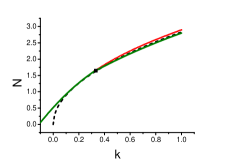
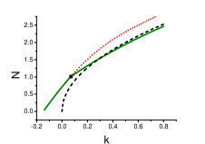
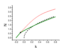
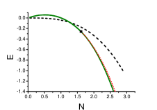
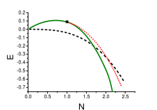
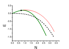
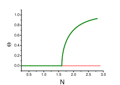
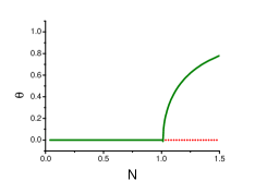
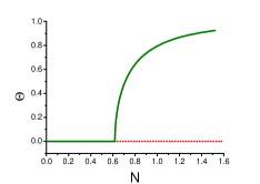
Figure 4: (Color online) Families of symmetric and asymmetric modes, represented by curves for the norm vs. the propagation constant in panels (a-c), Hamiltonian vs. the norm in panels (d-f), and the asymmetry [defined per Eq. (15)] vs. the norm in panels (g-i). The left, middle, and right plots correspond, severally, to the height of the central barrier in potential (6) $A=0.05$, $0.2$, and $0.5$. Continuous (olive) and dotted (red) lines designate stable and unstable states, respectively. The dashed lines in the top and middle panels depict, for the sake of comparison, the $N(k)$ and $E(N)$ dependences for free-space solitons, given by Eq. (13). The square symbols in (a-f) designate the location of the bifurcation points.

The fact that the asymmetric modes, when they exists, have smaller values of $E$ for given $N$, hence they realize the system’s GS [see Figs. 4(d-f)], can be easily understood: having their center shifted from the layer occupied by the positive potential ($|x|<0.5$) to a region where $H=0$ [$0.5<|x|<3$, see Figs. 1 and 2], they obviously reduce the integral value of $E$. The same argument explains why, for given $k$, the asymmetric modes feature smaller $N$: having smaller overlap with the region of $H>0$, they need a smaller norm to compensate the shift of $k$ towards negative values induced by the positive potential, see Eq. (4).

Note that the families of states displayed in Figs. 4(a-c) comprise both $k<0$ and $k>0$, i.e., the leaky and trapped modes alike. In particular, the SSB bifurcation occurs at $k>0$ in panels 4(a,b), and at $k<0$ in (c) (in the latter case, the SSB sets in at $k=-0.100$, as shown for the same system in Fig. 3). A noteworthy fact is that the system features the competition of the two different mean-field phase transitions driven by the increase of $N$, i.e., the strength of the self-attraction: the transition from the quasi-bound (leaky) state to the self-trapped one, which was previously found in single-well elevated potentials Carr1 ; Carr2 , and the SSB in the DWP structure. Thus, in the cases shown in Figs. 4(a,b) the self-trapping transition happens first (at smaller $N$), while in Fig. 4(c) the SSB takes place prior to the onset of the self-trapping.

The values of the propagation constant and norm at the SSB bifurcation point are shown, as a function of the inner-barrier’s height $A$ [see Eq. (6)], in Fig. 5. In panel (5), the boundary between the SSB occurring with the delocalized and trapped modes ($k_{\mathrm{bif}}<0$ and $k_{\mathrm{bif}}>0$, respectively) is located at $A\approx 0.30$, the same value corresponding to the boundary designated by the square symbol in panel 5). That is, the SSB happens first (at smaller $N$) at $A>0.30$, while the transition to the self-trapping precedes the SSB at $A<0.30$.

Figure 5: Values of propagation constant $k$ (a), and total norm $N$ (b), at the SSB bifurcation point vs. the height of the inner barrier ($A$). The horiziontal line, $k=0$, in (a), and the square symbol in (b) designate the boundary between the trapped and leaky modes.

The fact that the SSB happens with the trapped and leaky modes, respectively, at small and large $A$, as seen in Fig. 5, is easy to explain: small $A$ implies strong linear coupling between the wave functions in the two barely separated wells, hence very large $N$ is required to induce the SSB, being far greater than the value of $N$ needed for the onset of the self-trapping, which is determined by the fixed parameters of the outer barrier in the DWP structure (6). On the contrary, large $A$ implies weak linear coupling between the strongly separated wells, hence the respective strength of the nonlinearity (measured by $N$), required for the SSB, is much smaller than the value necessary for the commencement of the self-trapping. These arguments clearly suggest that the same sequence of the SSB and self-trapping phase transitions should take place in generic DWP structures.

These arguments can be cast in a more definite form, if the central barrier in Eq. (6) is approximated by $H_{\mathrm{central}}(x)=A\delta(x)$, and the outer barriers are made impenetrable, similar to what is shown in Fig. 2(c). These conjectures replace the present model by the one for an infinitely deep potential box split by delta-functional barrier, which is the simplest model of the SSB NaturePhot2 ; Chili . In the limit of large $A$, the latter model predicts the following value of the norm at the SSB bifurcation point,

$$N_{\mathrm{bif}}\approx 8\pi^{2}/\left(3l^{2}A\right)$$ (16)

(see caption to Fig. 2 in Ref. NaturePhot2 ), where $l/2$ is the coordinate of the point at which the wave function vanishes (half-width of the infinitely deep box). In particular, one can identify $l\simeq 9$ for $A=0.5$ in Fig. 2(b), hence Eq. (16) yields $N_{\mathrm{bif}}~{}\simeq 0.65$, while the respective numerical  value in Fig. 5(b) is $N_{\mathrm{bif}}~{}\approx 0.62$, which implies a reasonable agreement for the present (not really large) value of $A$.

IV Evolution of unstable symmetric states

Conclusions concerning the stability and instability of the symmetric and asymmetric modes, presented in Fig. 4, were verified, in addition to the computation of eigenvalues for small perturbations, by direct simulations, performed by dint of the finite-difference algorithm. The instability development of unstable symmetric states was catalyzed by adding small initial symmetry-breaking perturbations to them. This was done for the unstable symmetric states with both $k>0$ and for $k<0$, i.e., self-trapped and leaky ones. Typical examples are displayed in Fig. 6, in which the unstable symmetric modes feature single- and double (split)-peak shapes at small and large values of the inner-barrier’s height, $A=0.05$ and $A=0.5$, respectively (in the top and bottom rows of the figure).

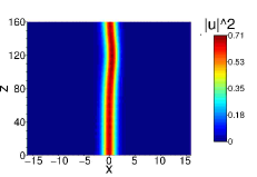
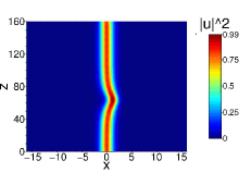
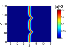
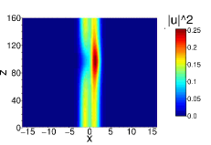
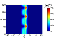
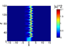
Figure 6: (Color online) The evolution of unstable symmetric states is displayed in panels (a-c) for potential (6) with $A=0.05$, and in panels (d)-(f) for $A=0.5$, the corresponding SSB bifurcations taking place at positive $k_{\mathrm{bif}}$, viz., $k_{\mathrm{bif}}\approx 0.313$ (a-c), and negative $k_{\mathrm{bif}}$, viz., $k_{\mathrm{bif}}\approx-0.100$ (d-f), respectively: (a) $k=0.314$; (b) $k=0.40;$ (c) $k=0.90$; (d) $k=-0.08$; (e) $k=-0.01$; (f) $k=0.30$ [$k>0$ in (f) is chosen to display unstable evolution which takes place far from the bifurcation point]. The instability gets stronger with the increae of $k$, i.e., moving from the left panels to the right ones.

As mentioned above, the instability of symmetric states is accounted for by pure imaginary eigenfrequencies, hence the originally developing instability is not oscillatory. However, the nonlinearity makes the unstable dynamics oscillatory, as seen in Fig. 6. In other words, the unstable symmetric modes spontaneously develop bosonic Josephson oscillations. Close to the instability onset, the effective oscillation period is very large (as it diverges precisely at the onset point), gradually decreasing deeper into the instability region. The dynamical symmetry breaking induced by the weak and moderate instability is incomplete, leading to periodic oscillations between the original symmetric state and a new asymmetric one, as observed in Fig. 6(a-e). Stronger instability causes complete symmetry breaking, replacing the symmetric state by an irregularly vibrating asymmetric mode, as seen in Fig. 6(f).

It is relevant to note the difference between the oscillatory regimes generated by the instability of self-trapped and leaky modes. Indeed, while Fig. 6(c) demonstrates that the shape of the oscillating mode is sharp in the former case, the shape is fuzzy in Fig. 6(e) because it involves an essential radiation component in the case when the underlying unstable mode is a leaky one.

V Collisions of free solitons with the quasi-double-well potential structure

In addition to the analysis of the stationary states performed above, it is also relevant to consider collisions of free solitons with the elevated DWP structure. For this purpose, the initial soliton was created as the tilted (moving) version of the static one given by Eqs. (3) and (14),

$$\psi\left(x,z\right)=\sqrt{2k}\exp\left(i\left(k-c^{2}/2\right)z+icx\right)\text{{sech}}\left(\sqrt{2k}\left(\left(x-x_{0}\right)-cz\right)\right),$$ (17)

where $c$ is a real tilt (velocity), and $x_{0}$ is the initial position of the soliton, chosen far enough from the localized potential structure (we here take $x_{0}=-15$). Generic findings are produced here for incident solitons with $k=3,$ the corresponding norm being

$$N=2\sqrt{2k}\approx 4.90,$$ (18)

according to Eq. (13), other values of $N$ giving similar results.

Figure 7 presents a parameter chart for three different outcomes of the collisions, produced by varying the height of the outer barriers, $H_{0}$ in Eq. (8), and tilt $c$ in Eq. (17). In the region designated as (1), i.e., for $c$ small and/or $H_{0}$ large enough, the incident soliton bounces back the left outer barrier, as shown in Fig. 8 for $H_{0}=0.6$ and $c=0.8$. At larger $c$, in a relatively narrow region (2) of Fig. 7, the soliton gets captured inside the potential structure, which resembles the previously explored possibility of capturing an incident Bragg-grating soliton by a cavity formed by two locally repulsive defects cavity . Similar to that setting, the trapped soliton performs shuttle motion between the outer and inner potential barriers, as shown in Fig. 8, for $H_{0}=0.6$ and $c=1.15$. The shuttle dynamical regime is an essential addition to the stationary states revealed by the analysis presented above. At still larger $c$, but yet staying within the boundaries of the narrow region (2), the shuttle motion of the trapped soliton becomes irregular, see Fig. 8 for $H_{0}=1.3$ and $c=1.8$.

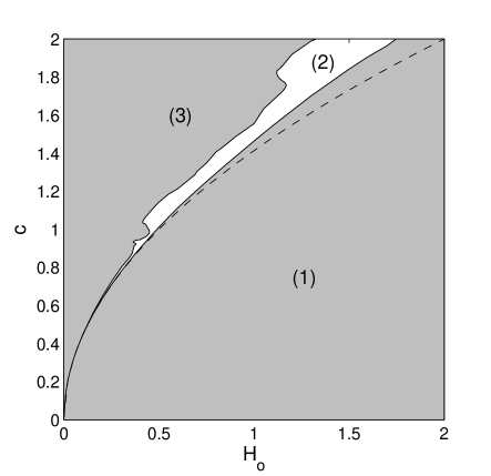
Figure 7: The chart of outcomes of collisions of free solitons, launched with tilt $c$ [see Eq. (17)], with potential structure (8), in the plane of $\left(H_{0},c\right)$. The norm of the incident soliton is fixed as per Eq. (18). In this figure, the width of the outer potential barriers is $W_{0}=4$. In region (1), the soliton bounces back from the left outer barrier. Region (2) refers to trapping the soliton inside the potential structure, where it performs shuttle motion. In region (3), the incident soliton passes the structure. The dashed line is the analytical prediction produced by Eq. (21).

In region (3), the initial tilt, $c$, is large enough for the soliton to pass the potential structure, see an example in Fig. 8 for $H_{0}=0.6$ and $c=1.5$. Another option admitted by this scenario is shown in Fig. 8, where the soliton passes the left outer barrier, bounces back from the inner one, and escapes in the reverse direction, passing the left outer barrier again. Naturally, this collision pattern is common for lower $H_{0}$, when the outer barriers are lower than the inner one, which plays the role of a strong “bouncer”. Furthermore, at $c>1.85$, the incident soliton splits into two fragments, one escaping and the other one staying in a chaotically evolving trapped state, see an example in Fig. 8, for $H_{0}=1.2$ and $c=1.92$.

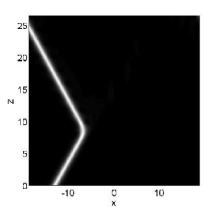
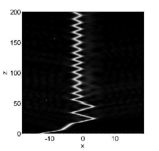
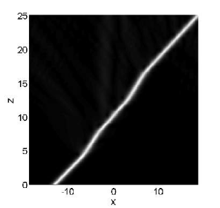
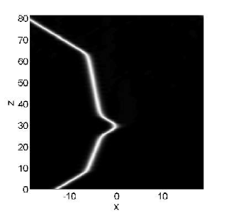
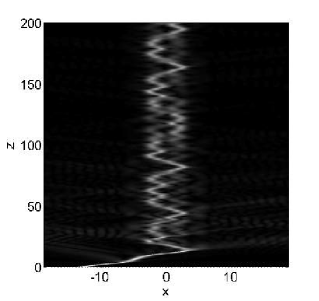
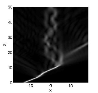
Figure 8: Generic examples of outcomes of collisions of the soliton with the double-well potential structure (8), for $N=4.90$ ($k=3$), $W_{0}=4$, and different heights of the outer initial barriers, $H_{0}$, and different tilts $c$ of the incident soliton: (a) $[H_{0}=0.6,c=0.8]$, (b) $[H_{0}=0.6,c=1.15]$, (c) $[H_{0}=0.6,c=1.5]$, (d) $[H_{0}=0.3,c=0.8]$, (e) $[H_{0}=1.3,c=1.8]$, (f) $[H_{0}=1.2,c=1.92]$, see further explanations in the text.

Collision scenarios were also explored by varying width $W_{0}$ of the outer barriers, while keeping their height constant, $H_{0}=1$, as well as characteristics of the inner barrier and the distance between the barriers, see Eq. (8). The respective results, for the same incident soliton as used above ($k=3$, $N=4.90$), are summarized in Fig. 9, where regions (1)-(3) have the same meaning as their counterparts in Fig. 7.

In the latter case, the results may be classified into three outcomes of the collision, depending on $W_{0}$. The first outcome occurs at $0<W_{0}<0.8$. It is characterized by a rapidly growing region of the shuttle motion of the trapped soliton [region (2)], and sharp transitions between the three evolution scenarios, $(1)\leftrightarrow(2)$, $(2)\leftrightarrow(3)$. The second outcome, which was observed in the range of $0.8<W_{0}<1.8$ (in this case, $W_{0}$ is, roughly, close to the width of the incident soliton), is distinguished by gradual transitions between the scenarios. That means that, for certain values of $c$, the soliton does not fully bounce from the barrier, nor penetrates it, but rather splits into two segments, one of which escapes, while the other remains trapped. In this case, both the upper and lower boundaries of region (2) represent tilts at which the soliton is split into equal fragments. An example of such an outcome is shown in Fig. 10, for $W_{0}=1.2$ and $c=1.66$. The third outcome, which is observed at $W_{0}>1.8$, is distinguished by the fact that the variation of $W_{0}$ almost does not affect the soliton’s motion. In contrast to the second outcome, and similar to the first one, the respective transitions between the regions are sharp.

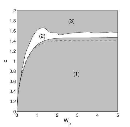
Figure 9: The same as in Fig. 7, but varying the width of the outer potential barriers, $W_{0}$, while their height is fixed, $H_{0}=1$. The dashed curve shows the analytical prediction for the boundary of area (1) given by Eq. (20).

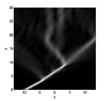
Figure 10: Outcomes of the collisions, for $W_{0}=1.2$ and $c=1.66$. In this borderline example, the soliton hits the right (second) outer potential barrier and splits into two fragments, one escaping and the other one staying trapped in the potential structure.

It is easy to explain the parabolic boundary of region (1) in Fig. 7, as well as the boundary of the same region in Fig. 9, using the perturbation theory for NLS solitons, which treats them as quasi-particles with mass $N$ RMP . Indeed, the kinetic energy of the soliton is $E_{\mathrm{kin}}=(N/2)c^{2}$, while the height of the outer potential barrier for the quasi-particle, $E_{0}$, can be obtained from the third term in expression (5), assuming that the soliton’s center is located at the midpoint of the potential barrier:

$$E_{0}=H_{0}\int_{-W_{0}/2}^{+W_{0}/2}u_{\mathrm{sol}}^{2}\left(x^{\prime}\right)dx^{\prime}=H_{0}N\tanh\left(\frac{1}{4}W_{0}N\right),$$ (19)

where $u_{\mathrm{sol}}$ is the solitons’s profile (14), $x^{\prime}\equiv x-\left(3+W_{0}/2\right)$ [see Eq. (8)], and the result is expressed in terms of the soliton’s norm, as per Eq. (13). Next, equating $E_{\mathrm{kin}}$ to $E_{0}$ predicts that the boundary between the rebound and passage corresponds to

$$c_{\mathrm{cr}}=\sqrt{2H_{0}\tanh\left(\frac{1}{4}W_{0}N\right)}.$$ (20)

In particular, the respective prediction for dependence $c_{\mathrm{cr}}(H_{0})$ corresponding to the case displayed in Fig. 7, with $W_{0}=4$ and $N$ fixed as per Eq. (18), simplifies to

$$c_{\mathrm{cr}}=\sqrt{2H_{0}}.$$ (21)

Figure 7 demonstrates that Eq. (21) predicts the parabolic boundary of region (1) quite accurately, a discrepancy at large $H_{0}$ being explained by the fact that the collision with the tall barrier causes a deformation of the soliton’s shape. Further, the full analytical expressions (20) predicts the boundary of the same region in Fig. 9 well enough too.

As concerns the trapping regime in area (2) of Figs. 7 and 9, it is explained by the fact that, while slowly passing the left barrier, and then passing the inner one, the soliton with the initial tilt slightly exceeding value (20) suffers radiation losses due to its deceleration and acceleration. The losses cause a drop in the kinetic energy below the level necessary for clearing the right barrier. A feature which relates the trapping and splitting to the leaky modes considered above is tunneling of the radiation across the outer potential barriers, which can be seen, in particular, in Figs. 8(b,e,f).

VI Conclusions

We have extended the known possibility of the stabilization of leaky modes in quasi-trapping potentials by means of the self-attractive nonlinearity. Unlike the previously studied single-well potential, we have introduced the spatially symmetric DWP (double-well potential) with the elevated floor, embedded into the potential barrier. The setting can be implemented in nonlinear optical waveguides and BEC. The new possibility offered by this system is the competition of two phase transitions of the second kind, described in the mean-field approximation: the onset of the self-trapping of the leaky modes, and the SSB (spontaneous symmetry breaking) of both true bound states and leaky modes, under the action of the self-attractive nonlinearity. With the increase of the norm of the wave field (which determines the nonlinearity strength), the former or latter transition happens first if the central barrier of the DWP structure is, respectively, low or tall. These conclusions are generic, as they do not depend on details of the DWP structure. New effects are revealed by the consideration of the SSB of the leaky modes: asymmetry of radiation tails, which are parts of these modes, and the commensurability-incommensurability interplay between the radiation wavelength and the total size of the system, into which the DWP is embedded. Systematic results have been produced in the numerical form, and their basic features were explained with the help of analytical considerations. The simulations demonstrate that unstable symmetric modes initiate Josephson oscillations. Collisions of freely moving solitons with the DWP structure were studied in a systematic form too, revealing various generic outcomes of the collisions, boundaries between which were explained in the analytical form. In particular, in addition to the stationary states with the unbroken and broken symmetry, the collisions reveal the dynamical mode, in the form of a soliton which performs persistent shuttle motion in the DWP structure.

Relevant possibilities for the extension of the analysis reported in this work may be offered by two-component systems, as well as by a two-dimensional generalization of the present setting. On the other hand, the results produced by the competition of the mean-field phase transitions suggest that it may be interesting too to consider quantum phase transitions in a many-body bosonic state with attractive inter-particle interactions, loaded into the DWP.

VII Acknowledgment

M.T. and B.A.M. acknowledge partial support from the National Science Center of Poland in the framework of the HARMONIA Program, No. 2012/06/M/ST2/00479. K.B.Z. acknowledges support from the National Science Center of Poland through Project ETIUDA No. 2013/08/T/ST2/00627.

References

- (1) D. Landau and E. M. Lifshitz, Quantum Mechanics (Nauka Publishers: Mosocw, 1974).
- (2) R. Englman, The Jahn-Teller Effect in Molecules and Crystals (Wiley-Interscience: London, 1972).
- (3) S. Giorgini, L. P. Pitaevskii, and S. Stringari, Rev. Mod. Phys. 80, 1215 (2008); H. T. C. Stoof, K. B. Gubbels, and D. B. M. Dickrsheid, Ultracold Quantum Fields (Springer: Dordrecht, 2009).
- (4) Y. S. Kivshar and G. P. Agrawal, Optical Solitons: From Fibers to Photonic Crystals (Academic Press: San Diego, 2003).
- (5) Spontaneous Symmetry Breaking, Self-Trapping, and Josephson Oscillations, Editor: B. A. Malomed (Springer-Verlag: Berlin and Heidelberg, 2013).
- (6) E. B. Davies, “Symmetry breaking in a non-linear Schrödinger equation”, Commun. Math. Phys. 64, 191-210 (1979).
- (7) J. C. Eilbeck, P. S. Lomdahl, and A. C. Scott, “The discrete self-trapping equation”, Physica D 16, 318-338 (1985).
- (8) G. L. Alfimov, P. G. Kevrekidis, V. V. Konotop, and M. Salerno, “Wannier functions analysis of the nonlinear Schrödinger equation with a periodic potential”, Phys. Rev. E 66, 046608 (2002).
- (9) D. Ananikian and T. Bergeman, “Gross-Pitaevskii equation for Bose particles in a double-well potential: Two-mode models and beyond”, Phys. Rev. A 73, 013604 (2006).
- (10) G. J. Milburn, J. Corney, E. M. Wright, and D. F. Walls, “Quantum dynamics of an atomic Bose-Einstein condensate in a double-well potential”, Phys. Rev. A 55, 4318-4324 (1997).
- (11) A. Smerzi, S. Fantoni, S. Giovanazzi, and S. R. Shenoy, “Quantum coherent atomic tunneling between two trapped Bose-Einstein condensates”, Phys. Rev. Lett. 79, 4950-4953 (1997).
- (12) G. Iooss and D. D. Joseph, Elementary Stability and Bifurcation Theory (Springer: New York, 1980).
- (13) M. Matuszewski, B. A. Malomed, and M. Trippenbach, “Spontaneous symmetry breaking of solitons trapped in a double-channel potential”, Phys. Rev. A 75, 063621 (2007).
- (14) V. M. Pérez-García, H. Michinel, and H. Herrero, “Bose-Einstein solitons in highly asymmetric traps”, Phys. Rev. A 57, 3837-3842 (1998).
- (15) C. Paré and M. Florjańczyk, “Approximate model of soliton dynamics in all-optical couplers”, Phys. Rev. A 41, 6287-6295 (1990); A. I. Maimistov, “Propagation of a light pulse in nonlinear tunnel-coupled optical waveguides”, Sov. J. Quantum Electron. 21, 687-690 (1991); P. L. Chu, B. A. Malomed, and G. D. Peng, “Soliton switching and propagation in nonlinear fiber couplers: analytical results”, J. Opt. Soc. Am. B 10, 1379-1385 (1993); N. Akhmediev and A. Ankiewicz, “Novel soliton states and bifurcation phenomena in nonlinear fiber couplers”, Phys. Rev. Lett. 70, 2395-2398 (1993); B. A. Malomed, I. M. Skinner, P. L. Chu, and G. D. Peng, “Symmetric and asymmetric solitons in twin-core nonlinear optical fibers”, Phys. Rev. E 53, 4084-4091 (1996).
- (16) A. W. Snyder, D. J. Mitchell, L. Poladian, D. R. Rowland, and Y. Chen, “Physics of nonlinear fiber couplers”, J. Opt. Soc. Am. B 8, 2102-2118 (1991).
- (17) G. Schön and A. D. Zaikin, “Quantum coherent effects, phase transitions, and the dissipative dynamics of ultra small tunnel junctions”, Phys. Rep. 198, 237-412 (1990).
- (18) A. V. Ustinov, “Solitons in Josephson junctions”, Physica D 123, 315-329 (1998).
- (19) S. Raghavan, A. Smerzi, S. Fantoni, and S. R. Shenoy, “Coherent oscillations between two weakly coupled Bose-Einstein condensates: Josephson effects, oscillations, and macroscopic quantum self-trapping”, Phys. Rev. A 59, 620-633 (1999); A. Smerzi, and S. Raghavan, Phys. Rev. A 61, 063601 (2000); R. Burioni, D. Cassi, I. Meccoli, M. Rasetti, S. Regina, P. Sodano, and A. Vezzani, “Bose-Einstein condensation in inhomogeneous Josephson arrays”, Europhys. Lett. 52, 251-256 (2000); Gati and M. K. Oberthaler, “A bosonic Josephson junction”, J. Phys. B At. Mol. Opt. Phys. 40, R61-R89 (2007).
- (20) M. Albiez, R. Gati, J. Fölling, S. Hunsmann, M. Cristiani, and M. K. Oberthaler, “Direct observation of tunneling and nonlinear self-trapping in a single bosonic Josephson junction”, Phys. Rev. Lett. 95, 010402 (2005).
- (21) P. G. Kevrekidis, Z. Chen, B. A. Malomed, D. J. Frantzeskakis, and M. I. Weinstein, “Spontaneous symmetry breaking in photonic lattices: Theory and experiment”, Phys. Lett. A 340, 275-280 (2005).
- (22) T. Heil, I. Fischer, W. Elsässer, J. Mulet, and C. R. Mirasso, “Chaos synchronization and spontaneous symmetry-breaking in symmetrically delay-coupled semiconductor lasers”. Phys. Rev. Lett. 86, 795-798 (2001).
- (23) P. Hamel, S. Haddadi, F. Raineri, P. Monnier, G. Beaudoin, I. Sagnes, A. Levenson, and A. M. Yacomotti, “Spontaneous mirror-symmetry breaking in a photonic molecule”, Nature Phot. 9, 311-315 (2015).
- (24) B. A. Malomed, “Symmetry breaking in laser cavities”, Nature Phot. 9, 287-289 (2015).
- (25) B. A. Malomed, “Spontaneous symmetry breaking in nonlinear systems: An overview and a simple model”, in: Nonlinear Dynamics: Materials, Theory and Experiments (Springer Proceedings in Physics, vol. 173, 2016), ed. by M. Tlidi and M. Clerc, pp. 97-112.
- (26) M. Liu, D. A. Powell1, I. V. Shadrivov, M. Lapine, and Y. S. Kivshar, “Spontaneous chiral symmetry breaking in metamaterials”, Nature Comm. 5, 4441 (2014).
- (27) N. Moiseyev, L. D. Carr, B. A. Malomed, and Y. B. Band, “Transition from resonances to bound-states in nonlinear systems: application to Bose-Einstein condensates”, J. Phys. B 37, L193 (2004).
- (28) L. D. Carr, M. J. Holland, and B. A. Malomed, “Macroscopic quantum tunneling of Bose-Einstein condensates in a finite potential well”, J. Phys. B 38, 3217-3231 (2005).
- (29) H. J. Lipkin, N. Meshkov, and A. J. Glick, “Validity of many-body approximation methods for a solvable model. I. Exact solutions and perturbation theory”, NucI. Phys. 62, 188-198 (1965); V. V. Ulyanov and O. B. Zaslavskii, “New methods in the theory of quantum spin systems”, Phys. Rep. 216, 179-251 (1992).
- (30) G. E. Astrakharchik and B. A. Malomed, “Quantum versus mean-field collapse in a many-body system”, Phys. Rev. A 92, 043632 (2015).
- (31) H. Sakaguchi and B. A. Malomed, “Suppression of the quantum-mechanical collapse by repulsive interactions in a quantum gas”, Phys. Rev. A 83, 013607 (2011).
- (32) D. Kip, “Photorefractive waveguides in oxide crystals: fabrication, properties, and applications”, Appl. Phys. B - Lasers and Optics 67, 131-150 (1998); F. Chen, X.-L. Wang, and K.-M. Wang, “Development of ion-implanted optical waveguides in optical materials: A review”, Opt. Materials 29, 1523-1542 (2007).
- (33) T. Schumm, S. Hofferberth, L. M. Andersson, S. Wildermuth, S. Groth, I. Bar-Joseph, J. Schmiedmayer, and P. Kruger, “Matter-wave interferometry in a double well on an atom chip”, Nature Phys. 1, 57-62 (2005); S. Hofferberth, I. Lesanovsky, B. Fischer, J. Vedu, and J. Schmiedmayer, “Radiofrequency-dressed-state potentials for neutral atoms”, ibid. 2, 710-716 (2006).
- (34) M. Ya. Azbel and B. A. Malomed, “Possibility for time-scale-invariant relaxation in tunneling”, Phys. Rev. Lett. 71, 1617-1620 (1993).
- (35) M. Vakhitov and A. Kolokolov, “Stationary solutions of the wave equation in a medium with nonlinearity saturation”, Radiophys. Quantum Electron. 16, 783 (1973).
- (36) L. Bergé, “Wave collapse in physics: principles and applications to light and plasma waves”, Phys. Rep. 303, 259-370 (1998); G. Fibich and G. Papanicolaou, “Self-focusing in the perturbed and unperturbed nonlinear Schrödinger equation in critical dimension”,SIAM J. Appl. Math. 60, 183-240 (1999); E. A. Kuznetsov and F. Dias, “Bifurcations of solitons and their stability”,Phys. Rep. 507, 43-105 (2011).
- (37) P. Y. P. Chen, B. A. Malomed, and P. L. Chu, “Trapping Bragg solitons by a pair of defects”, Phys. Rev. E 71, 066601 (2005).
- (38) Y. S. Kivshar and B. A. Malomed, “Dynamics of solitons in nearly integrable systems”, Rev. Mod. Phys. 89, 763-915 (1989).