Visual descriptors for content-based retrieval of remote sensing images

Abstract

In this paper we present an extensive evaluation of visual descriptors for the content-based retrieval of remote sensing (RS) images. The evaluation includes global hand-crafted, local hand-crafted, and Convolutional Neural Network (CNNs) features coupled with four different Content-Based Image Retrieval schemes. We conducted all the experiments on two publicly available datasets: the 21-class UC Merced Land Use/Land Cover (LandUse) dataset and 19-class High-resolution Satellite Scene dataset (SceneSat). The content of RS images might be quite heterogeneous, ranging from images containing fine grained textures, to coarse grained ones or to images containing objects. It is therefore not obvious in this domain, which descriptor should be employed to describe images having such a variability. Results demonstrate that CNN-based features perform better than both global and and local hand-crafted features whatever is the retrieval scheme adopted. Features extracted from SatResNet-50, a residual CNN suitable fine-tuned on the RS domain, shows much better performance than a residual CNN pre-trained on multimedia scene and object images. Features extracted from NetVLAD, a CNN that considers both CNN and local features, works better than others CNN solutions on those images that contain fine-grained textures and objects.

1 Introduction

The recent availability of a large amount of remote sensing (RS) images is boosting the design of systems for their management. A conventional RS image management system usually exploits high-level features to index the images such as textual annotations and metadata Datta et al. (2008). In the recent years, researchers are focusing their attention on systems that exploit low-level features extracted from images for their automatic indexing and retrieval  Jain and Healey (1998). These types of systems are known as Content-Based Image Retrieval (CBIR) systems and they have demonstrated to be very useful in the RS domain Demir and Bruzzone (2015); Aptoula (2014); Ozkan et al. (2014); Yang and Newsam (2013); Zajić et al. (2007).

The CBIR systems allow to search and retrieve images that are similar to a given query image Smeulders et al. (2000); Datta et al. (2008). Usually their performance strongly depends on the effectiveness of the features exploited for representing the visual content of the images Smeulders et al. (2000). The content of RS images might be quite heterogeneous, ranging from images containing fine grained textures, to coarse grained ones or to images containing objects Yang and Newsam (2010); Dai and Yang (2011). It is therefore not obvious in this domain, which descriptor should be employed to describe images having such a variability.

In this paper we compare several visual descriptors in combination with four different retrieval schemes. Such descriptors can be grouped in two classes. The first class includes traditional global hand-crafted descriptors that were originally designed for image analysis and local hand-crafted features that were originally designed for object recognition. The second class includes features that correspond to intermediate representations of Convolutional Neural Networks (CNNs) trained for generic object and/or scene and RS image recognition.

To reduce the influence of the retrieval scheme on the evaluation of the features we investigated the features coupled with four different image retrieval schemes. The first one, that is also the simplest one, is a basic image retrieval system that takes one image as input query and returns a list of images ordered by their degree of feature similarity. The second and the third ones, named pseudo and manual Relevance Feedback (RF), extend the basic approach by expanding the initial query. The Pseudo RF scheme uses the $n$ most similar images to the initial query, for re-querying the image database. The final result is obtained by combining the results of each single query. In the manual RF, the set of relevant images is suggested by the user which evaluates the result of the initial query. The last scheme considered is named active-learning-based RF Demir and Bruzzone (2015). It exploits Support Vector Machines (SVM) to classify relevant and not relevant images on the basis of the user feedback.

For the sake of completeness, for the first three retrieval schemes we considered different measure of similarity, such as Euclidean, Cosine, Manhattan, and $\chi^{2}$-square, while for the active-learning-based RF scheme we considered the histogram intersection as similarity measure, as proposed by the original authors Demir and Bruzzone (2015).

We conducted all the experiments on two publicly available datasets: the 21-class UC Merced Land Use/Land Cover dataset Yang and Newsam (2010) (LandUse) and 19-class High-resolution Satellite Scene dataset Dai and Yang (2011) (SatScene). Evaluations exploit several computational measures in order to quantify the effectiveness of the features. To make the experiments replicable, we made publicly available all the visual descriptors calculated as well as the scripts for making the evaluation of all the image retrieval schemes .

The rest of the paper is organized as follows: Section 2 reviews the most relevant visual descriptors and retrieval schemes; Section  3 describes the data, visual descriptors, retrieval schemes evaluated and the experimental setup; Section 4 reports and analyzes the experimental results; finally, Section 5 presents our final considerations and discusses some new directions for our future research.

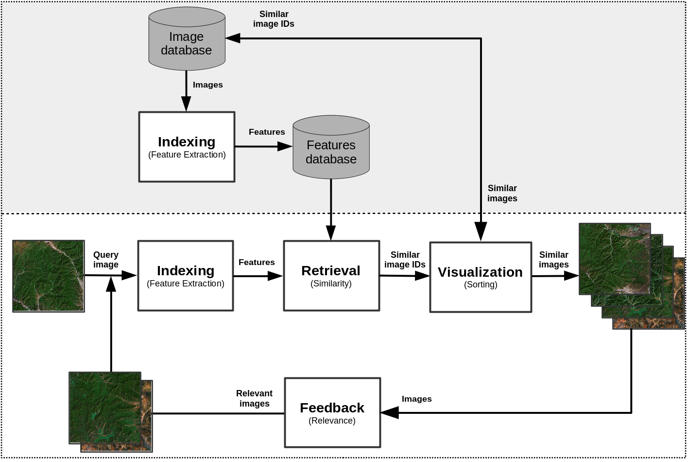
Figure 1: Main components of a CBIR system.

2 Background and Related Works

A typical Content-Based Image Retrieval (CBIR) system is composed of four main parts Smeulders et al. (2000); Datta et al. (2008), see Fig. 1:

1. The Indexing, also called feature extraction, module computes the visual descriptors that characterize the image content. Given an image, these features are usually pre-computed and stored in a database of features;

2. The Retrieval module, given a query image, finds the images in the database that are most similar by comparing the corresponding visual descriptors.

3. The Visualization module shows the images that are most similar to a given query image ordered by the degree of similarity.

4. The Relevance Feedback module makes it possible to select relevant images from the subset of images returned after an initial query. This selection can be given manually by a user or automatically by the system.

2.1 Indexing

A huge variety of features have been proposed in literature for describing the visual content. They are often divided into hand-crafted features and learned features. Hand-crafted descriptors are features extracted using a manually predefined algorithm based on the expert knowledge. Learned descriptors are features extracted using Convolutional Neural Networks (CNNs).

Global hand-crafted features describe an image as a whole in terms of color, texture and shape distributions Mirmehdi, Xie, and Suri (2009). Some notable examples of global features are color histograms Novak, Shafer et al. (1992), spatial histogram Wang, Wu, and Yang (2010), Gabor filters Manjunath and Ma (1996), co-occurrence matrices Arvis et al. (2004); Haralick (1979), Local Binary Patterns (LBP) Ojala, Pietikäinen, and Mänepää (2002), Color and Edge Directivity Descriptor (CEDD) Chatzichristofis and Boutalis (2008), Histogram of Oriented Gradients (HOG) Junior et al. (2009), morphological operators like granulometries information Bosilj et al. (2016); Aptoula (2014); Hanbury, Kandaswamy, and Adjeroh (2005), Dual Tree Complex Wavelet Transform (DT-CWT) Bianconi et al. (2011); Barilla and Spann (2008) and GIST Oliva and Torralba (2001). Readers who would wish to deepen the subject can refer to the following papers Rui, Huang, and Chang (1999); Deselaers, Keysers, and Ney (2008); Liu and Yang (2013); Veltkamp, Burkhardt, and Kriegel (2013).

Local hand-crafted descriptors like Scale Invariant Feature Transform (SIFT) Lowe (2004); Bianco et al. (2015) provide a way to describe salient patches around properly chosen key points within the images. The dimension of the feature vector depends on the number of chosen key points in the image. A great number of key points can generate large feature vectors that can be difficult to be handled in the case of a large-scale image retrieval system. The most common approach to reduce the size of feature vectors is the Bag-of-Visual Words (BoVW) Sivic and Zisserman (2003); Yang and Newsam (2010). This approach has shown excellent performance not only in image retrieval applications Deselaers, Keysers, and Ney (2008) but also in object recognition Grauman and Leibe (2010), image classification Csurka et al. (2004) and annotation Tsai (2012). The idea underlying is to quantize by clustering local descriptors into visual words. Words are then defined as the centers of the learned clusters and are representative of several similar local regions. Given an image, for each key point the corresponding local descriptor is mapped to the most similar visual word. The final feature vector of the image is represented by the histogram of the its visual words.

CNNs are a class of learnable architectures used in many domains such as image recognition, image annotation, image retrieval etc Schmidhuber (2015). CNNs are usually composed of several layers of processing, each involving linear as well as non-linear operators, that are learned jointly, in an end-to-end manner, to solve a particular tasks. A typical CNN architecture for image classification consists of one or more convolutional layers followed by one or more fully connected layers. The result of the last full connected layer is the CNN output. The number of output nodes is equal to the number of image classes Krizhevsky, Sutskever, and Hinton (2012).

A CNN that has been trained for solving a given task can be also adapted to solve a different task. In practice, very few people train an entire CNN from scratch, because it is relatively rare to have a dataset of sufficient size. Instead, it is common to take a CNN that is pre-trained on a very large dataset (e.g. ImageNet, which contains 1.2 million images with 1000 categories Deng et al. (2009)), and then use it either as an initialization or as a fixed feature extractor for the task of interest Razavian et al. (2014); Vedaldi and Lenc (2014). In the latter case, given an input image, the pre-trained CNN performs all the multilayered operations and the corresponding feature vector is the output of one of the fully connected layers Vedaldi and Lenc (2014). This use of CNNs have demonstrated to be very effective in many pattern recognition applications Razavian et al. (2014).

2.2 Retrieval

A basic retrieval scheme takes as input the visual descriptor corresponding to the query image perfomed by the user and it computes the similarity between such a descriptor and all the visual descriptors of the database of features. As a result of the search, a ranked list of images is returned to the user. The list is ordered by a degree of similarity, that can be calculated in several ways Smeulders et al. (2000): Euclidean distance (that is the most used), Cosine similarity, Manhattan distance, $\chi^{2}$-square distance, etc. Brinke, Squire, and Bigelow (2004).

2.3 Relevance Feedback

In some cases visual descriptors are not able to completely represent the image semantic content. Consequently, the result of a CBIR system might be not completely satisfactory. One way to improve the performance is to allow the user to better specify its information need by expanding the initial query with other relevant images Rui et al. (1998); Hong, Tian, and Huang (2000); Zhou and Huang (2003); Li and Allinson (2013). Once the result of the initial query is available, the feedback module makes it possible to automatically or manually select a subset of relevant images. In the case of automatic relevance feedback (pseudo-relevance feedback) Baeza-Yates, Ribeiro-Neto et al. (1999), the top $n$ images retrieved are considered relevant and used to expand the query. In the case of manual relevance feedback (explicit relevance feedback (RF)) Baeza-Yates, Ribeiro-Neto et al. (1999), it is the user that manually selects $n$ relevant of images from the results of the initial query. In both cases, the relevance feedback process can be iterated several times to better capture the information need. Given the initial query image and the set of relevant images, whatever they are selected, the feature extraction module computes the corresponding visual descriptors and the corresponding queries are performed individually. The final set of images is then obtained by combining the ranked sets of images that are retrieved. There are several alternative ways in which the relevance feedback could implemented to expand the initial query. Readers who would wish to deepen on this topic can refer the following papers Zhou and Huang (2003); Li and Allinson (2013); Rui and Huang (2001).

The performance of the system when relevance feedback is used, strongly depends on the quality of the results achieved after the initial query. A system using effective features for indexing, returns a high number of relevant images in the first ranking positions. This makes the pseudo-relevance feedback effective and, in the case of manual relevance feedback, it makes easier to the user selecting relevant images within the result set.

Although there are several examples in the literature of manual RF Thomee and Lew (2012); Ciocca and Schettini (1999); Ciocca, Gagliardi, and Schettini (2001), since human labeling task is enormously boring and time consuming, these schemes are not practical and efficient in a real scenario, especially when huge archives of images are considered. Apart from the pseudo-RF, other alternatives to manual RF approach are the hybrid systems such as the systems based on supervised machine learning Demir and Bruzzone (2015); Pedronette, Calumby, and Torres (2015). This learning method aims at finding the most informative images in the archive that, when annotated and included in the set of relevant and irrelevant images (i.e., the training set), can significantly improve the retrieval performance Demir and Bruzzone (2015); Ferecatu and Boujemaa (2007). The Active-Learning-based RF scheme presented by Demir et al. Demir and Bruzzone (2015) is an example of hybrid scheme. Given a query, the user selects a small number of relevant and not relevant images that are used as training examples to train a binary classifier based on Support Vector Machines. The system iteratively proposes images to the user that assigns the relevance feedback. At each RF iteration the classifier is re-trained using a set of images composed of the initial images and the images from the relevance feedback provided by the user. After some RF iterations, the classifier is able to retrieve images that are similar to the query with a higher accuracy with respect to the initial query. At each RF iteration, the system suggests images to the user by following this strategy: 1) the system selects the $p$ most uncertain (i.e. ambiguous) images by taking the ones closest to the classifier hyperplanes; 2) the system selects the $h$ (with $h<p$) most diverse images from the highest density regions of the future space.

3 Methods and materials

Given an image database $\mathbf{D}$ composed of $M$ images, the most $k$ relevant images of $\mathbf{D}$ to a given query are the $k$ images that have the smallest distances between their feature vectors and the feature vector extracted from the query image. Let us consider $\mathbf{x}$ and $\mathbf{y}$ as the feature vectors extracted from the query image and a generic image of $\mathbf{D}$ respectively. The distance $d(\mathbf{x},\mathbf{y})$ between two vectors can be calculated by using several distance functions, here we considered: Euclidean, Cosine, Manhattan, and $\chi^{2}$-square.

In this work we evaluated:

1. several visual descriptors as described in Sect. 3.1;

2. different retrieval schemes as described in Sect. 3.2;

We conducted all the experiments on two publicly available datasets described in Sec. 3.3 for which the ground truth is known.

3.1 Visual descriptors

In this work we compared visual descriptors for content-based retrieval of remote sensing images. We considered a few representative descriptors selected from global and local hand-crafted and Convolutional Neural Networks approaches. In some cases we considered both color and gray-scale images. The gray-scale image $L$ is defined as follows: $L=0.299R+0.587G+0.114B$. All feature vectors have been $L^{2}$ normalized (they have been divided by its $L^{2}$-norm):

3.1.1 Global hand-crafted descriptors

• 256-dimensional gray-scale histogram (Hist L) Novak, Shafer et al. (1992);

• 512-dimensional Hue and Value marginal histogram obtained from the HSV color representation of the image (Hist H V) Novak, Shafer et al. (1992);

• 768-dimensional RGB and rgb marginal histograms (Hist RGB and Hist rgb) Pietikainen et al. (1996);

• 1536-dimensional spatial RGB histogram achieved from a RGB histogram calculated in different part of the image (Spatial Hist RGB) Novak, Shafer et al. (1992);

• 5-dimensional feature vector composed of contrast, correlation, energy, entropy and homogeneity extracted from the co-occurrence matrices of each color channel (Co-occ. matr.) Arvis et al. (2004); Hauta-Kasari et al. (1996);

• 144-dimensional Color and Edge Directivity Descriptor (CEDD) features. This descriptor uses a fuzzy version of the five digital filters proposed by the MPEG-7 Edge Histogram Descriptor (EHD), forming 6 texture areas. CEDD uses 2 fuzzy systems that map the colors of the image in a 24-color custom palette;

• 8-dimensional Dual Tree Complex Wavelet Transform (DT-CWT) features obtained considering four scales, mean and standard deviation, and three color channels (DT-CWT and DT-CWT L) Bianconi et al. (2011); Barilla and Spann (2008);

• 512-dimensional Gist features obtained considering eight orientations and four scales for each channel (Gist RGB) Oliva and Torralba (2001);

• 32-dimensional Gabor features composed of mean and standard deviation of six orientations extracted at four frequencies for each color channel (Gabor L and Gabor RGB) Bianconi et al. (2011); Bianconi and Fernández (2007);

• 264-dimensional opponent Gabor feature vector extracted as Gabor features from several inter/intra channel combinations: monochrome features extracted from each channel separately and opponent features extracted from couples of colors at different frequencies (Opp. Gabor RGB) Jain and Healey (1998);

• 580-dimensional Histogram of Oriented Gradients feature vector Junior et al. (2009). Nine histograms with nine bins are concatenated to achieve the final feature vector (HoG);

• 78-dimensional feature vector obtained calculating morphological operators (granulometries) at four angles and for each color channel (Granulometry) Hanbury, Kandaswamy, and Adjeroh (2005);

• 18-dimensional Local Binary Patterns (LBP) feature vector for each channel. We considered LBP applied to gray images and to color images represented in RGB  Mäenpää and Pietikäinen (2004). We selected the LBP with a circular neighbourhood of radius 2 and 16 elements, and 18 uniform and rotation invariant patterns. We set $w=16$ and $w=30$ for the LandUse and SceneSat datasets respectively (LBP L and LBP RGB).

3.1.2 Local hand-crafted descriptors

1. SIFT: We considered four variants of the Bag of Visual Words (BoVW) representation of a 128-dimensional Scale Invariant Feature Transform (SIFT) calculated on the gray-scale image. For each variant, we built a codebook of $1024$ visual words by exploiting images from external sources.

   The four variants are:

   • SIFT: $1024$-dimensional BoVW of SIFT descriptors extracted from regions at given key points chosen using the SIFT detector (SIFT);

   • Dense SIFT: $1024$-dimensional BoVW of SIFT descriptors extracted from regions at given key points chosen from a dense grid.

   • Dense SIFT (VLAD): $25\,600$-dimensional vector of locally aggregated descriptors (VLAD) Cimpoi et al. (2014).

   • Dense SIFT (FV):$40\,960$-dimensional Fisher’s vectors (FV) of locally aggregated descriptors Jégou et al. (2010).

2. LBP: We considered the Bag of Visual Words (BoVW) representation of Local Binary Patterns descriptor calculated on each channel of the RGB color space separately and then concatenated. LBP has been extracted from regions at given key points sampled from a dense grid every 16 pixels. We considered the LBP with a circular neighbourhood of radius 2 and 16 elements, and 18 uniform and rotation invariant patterns Cusano, Napoletano, and Schettini (2015). We set $w=16$ and $w=30$ for the LandUse and SceneSat respectively. Also in this case the codebook was built using an external dataset (Dense LBP RGB).

3.1.3 CNN-based descriptors

The CNN-based features have been obtained as the intermediate representations of deep convolutional neural networks originally trained for scene and object recognition. The networks are used to generate a visual descriptor by removing the final softmax nonlinearity and the last fully-connected layer. We selected the most representative CNN architectures in the state of the art Vedaldi and Lenc (2014); Szegedy et al. (2015); He et al. (2016); Arandjelovic et al. (2016) by considering a different accuracy/speed trade-off. All the CNNs have been trained on the ILSVRC-2015 dataset Russakovsky et al. (2015) using the same protocol as in Krizhevsky, Sutskever, and Hinton (2012). In particular we considered $4096$, $2048$, $1024$ and $128$-dimensional feature vectors as follows Razavian et al. (2014); Marmanis et al. (2016):

• BVLC AlexNet (BVLC AlexNet): this is the AlexNet trained on ILSVRC 2012 Krizhevsky, Sutskever, and Hinton (2012).

• BVLC Reference CaffeNet (BVLC Ref): a AlexNet trained on ILSVRC 2012, with a minor variation Vedaldi and Lenc (2014) from the version as described in Krizhevsky, Sutskever, and Hinton (2012).

• Fast CNN (Vgg F): it is similar to the one presented in Krizhevsky, Sutskever, and Hinton (2012) with a reduced number of convolutional layers and the dense connectivity between convolutional layers. The last fully-connected layer is 4096-dimensional Chatfield et al. (2014).

• Medium CNN (Vgg M): it is similar to the one presented in Zeiler and Fergus (2014) with a reduced number of filters in the convolutional layer four. The last fully-connected layer is 4096-dimensional Chatfield et al. (2014).

• Medium CNN (Vgg M-2048-1024-128): three modifications of the Vgg M network, with lower dimensional last fully-connected layer. In particular we used a feature vector of 2048, 1024 and 128 size Chatfield et al. (2014).

• Slow CNN (Vgg S): it is similar to the one presented in Sermanet et al. (2014) with a reduced number of convolutional layers, less filters in the layer five and the Local Response Normalization. The last fully-connected layer is 4096-dimensional Chatfield et al. (2014).

• Vgg Very Deep 19 and 16 layers (Vgg VeryDeep 16 and 19): the configuration of these networks has been achieved by increasing the depth to 16 and 19 layers, that results in a substantially deeper network than the ones previously Simonyan and Zisserman (2014).

• GoogleNet Szegedy et al. (2015) is a 22 layers deep network architecture that has been designed to improve the utilization of the computing resources inside the network.

• ResNet 50 is Residual Network. Residual learning framework are designed to ease the training of networks that are substantially deeper than those used previously. This network has 50 layers He et al. (2016).

• ResNet 101 is Residual Network made of 101 layers He et al. (2016).

• ResNet 152 is Residual Network made of 101 layers He et al. (2016).

Besides traditional CNN architectures, we evaluated the NetVLAD Arandjelovic et al. (2016). This architecture is a combination of a Vgg VeryDeep 16 Simonyan and Zisserman (2014) and a VLAD layer Delhumeau et al. (2013). The network has been trained for place recognition using a subset of a large dataset of multiple panoramic images depicting the same place from different viewpoints over time from the Google Street View Time Machine Torii et al. (2013).

To further evaluate the power of CNN-based descriptors, we have fine-tuned a CNN to the remote sensing domain. We have chosen the ResNet-50 which represents a good trade-off between depth and performance. This CNN demonstrated to be very effective on the ILSVRC 2015 (ImageNet Large Scale Visual Recognition Challenge) validation set with a top 1- recognition accuracy of about 80% He et al. (2016).

For the fine-tuning procedure we considered a very recent RS database  Xia et al. (2017), named AID, that is made of aerial image dataset collected from Google Earth imagery. This dataset is made up of the following 30 aerial scene types: airport, bare land, baseball field, beach, bridge, center, church, commercial, dense residential, desert, farmland, forest, industrial, meadow, medium residential, mountain, park, parking, playground, pond, port, railway station, resort, river, school, sparse residential, square, stadium, storage tanks and viaduct. The AID dataset has a number of 10000 images within 30 classes and about 200 to 400 samples of size 600$\times$ 600 in each class.

We did not train the ResNet-50 from the scratch on AID because the number of images for each class is not enough. We started from the pre-trained ResNet-50 on ILSVRC2015 scene image classification dataset Russakovsky et al. (2015). From the AID dataset we have selected 20 images for each class and the rest has been using for training. During the fine-tuning stage each image has been resized to $256\times 256$ and a random crop has been taken of $224\times 224$ size. We augmented data with the horizontal flipping. During the test stage we considered a single central $224\times 224$ crop from the $256\times 256$-resized image.

The ResNet-50 has been trained via stochastic gradient descent with a mini-batch of 16 images. We set the initial learning rate to 0.001 with learning rate update at every 2K iterations. The network has been trained within the Caffe Jia et al. (2014) framework on a PC equipped with a Tesla NVIDIA K40 GPU. The classification accuracy of the resulting SatResNet-50 fine-tuned with the AID dataset is 96.34% for the Top-1, and 99.34% for the Top-5.

In the following experiments, the SatResNet-50 is then used as feature extractor. The activations of the neurons in the fully connected layer are used as features for the retrieval of food images. The resulting feature vectors have size 2048 components.

3.2 Retrieval schemes

We evaluated and compared three retrieval schemes exploiting different distance functions, namely Euclidean, Cosine, Manhattan, and $\chi^{2}$-square and an active-learning-based RF scheme using the histogram intersection as distance measure. In particular, we considered:

1. A basic IR. This scheme takes a query as input and outputs a list of ranked similar images.

2. Pseudo-RF. This scheme considers the first $n$ images returned after the initial query as relevant. We considered different values of $n$ ranging between 1 and 10.

3. Manual RF. Since the ground truth is known, we simulated the human interaction by taking the first $n$ actual relevant images from the result set obtained after the initial query. We evaluated performance at different values of $n$ ranging between 1 and 10.

4. Active-Learning-based RF. We considered an Active-Learning-based RF scheme as presented by Demir et al. Demir and Bruzzone (2015). The RF scheme requires the interaction with the user that we simulated taking relevant and not relevant images from the ground-truth.

3.3 Remote Sensing Datasets

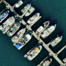
Figure 2: Examples from the 21-Class Land-Use/Land-Cover dataset. From the top left to bottom right: agricultural, airplane, baseball diamond, beach, buildings, chaparral, dense residential, forest, freeway, golf course, harbor, intersectionv, medium density residential, mobile home park, overpass, parking lot, river, runway, sparse residential, storage tanks, and tennis courts.

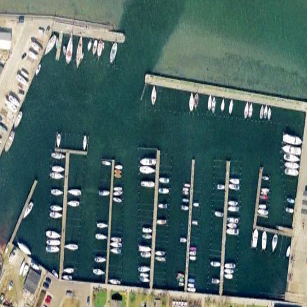
Figure 3: Examples from the 19-Class Satellite Scene dataset. From the top left to bottom right: airport, beach, bridge, commercial area, desert, farmland, football field, forest, industrial area, meadow, mountain, park, parking, pond, port, railway station, residential area, river and viaduct.

The 21-Class Land Use/Land Cover Dataset (LandUse) is a dataset of images of 21 land-use classes selected from aerial orthoimagery with a pixel resolution of 30 cm Yang and Newsam (2010). The images were downloaded from the United States Geological Survey (USGS) National Map of some US regions. . For each class, one hundred $256\times 256$ RGB images are available for a total of 2100 images. The list of 21 classes is the following: agricultural, airplane, baseball diamond, beach, buildings, chaparral, dense residential, forest, freeway, golf course, harbor, intersectionv, medium density residential, mobile home park, overpass, parking lot, river, runway, sparse residential, storage tanks, and tennis courts. Some examples are shown in Fig. 2.

The 19-Class Satellite Scene (SceneSat) dataset consists of 19 classes of satellite scenes collected from Google Earth (Google Inc.) . Each class has about fifty $600\times 600$ RGB images for a total of 1005 images  Dai and Yang (2011); Xia et al. (2010). following: airport, beach, bridge, commercial area, desert, farmland, football field, forest, industrial area, meadow, mountain, park, parking, pond, port, railway station, residential area, river and viaduct. An example of each class is shown in Fig. 3.

3.3.1 Differences between LandUse and SceneSat

The datasets used for the evaluation are quite different in terms of image size and resolution. LandUse images are of size $256\times 256$ pixels while SceneSat images are of size $600\times 600$ pixels. Fig. 4 displays some images from the same category taken from the two datasets. It is quite evident that the images taken from the LandUse dataset are at a different zoom level with respect to the images taken from the SatScene dataset. It means that objects in the LandUse dataset will be more easily recognizable than the objects contained in the SceneSat dataset, see the samples of harbour category in Fig. 4. The SceneSat images depict a larger land area than LandUse images. It means that the SceneSat images have a more heterogeneous content than LandUse images, see some samples from harbour, residential area and parking categories reported in Fig. 2 and Fig. 3. Due to these differences between the two considered datasets, we may expect that the same visual descriptors will have different performance across datasets, see Sec. 4.

(LandUse)	(SceneSat)	(LandUse)	(SceneSat)
Harbor		Forest

Figure 4: Comparison between images of the same classes between LandUse and SceneSat dataset.

3.4 Retrieval measures

Image retrieval performance has been assessed by using three state of the art measures: the Average Normalized Modified Retrieval Rank (ANMRR), Precision (Pr) and Recall (Re), Mean Average Precision (MAP) Manning, Raghavan, and Schütze (2008); Manjunath et al. (2001). We also adopted the Equivalent Query Cost (EQC) to measure the cost of making a query independently of the computer architecture.

3.4.1 Average Normalized Modified Retrieval Rank (ANMRR)

The ANMRR measure is the MPEG-7 retrieval effectiveness measure commonly accepted by the CBIR community Manjunath et al. (2001) and largely used by recent works on content-based remote sensing image retrieval Ozkan et al. (2014); Aptoula (2014); Yang and Newsam (2013). This metric considers the number and rank of the relevant (ground truth) items that appear in the top images retrieved. This measure overcomes the problem related to queries with varying ground-truth set sizes. The ANMRR ranges in value between zero to one with lower values indicating better retrieval performance and is defined as follows:

$$ANMRR=\frac{1}{NQ}\sum_{q=1}^{NQ}\frac{AVR(q)-0.5[1+NG(q)]}{1.25K(q)-0.5[1+NG(q)}.$$

$NQ$ indicates the number of queries $q$ performed. $NG(q)$ is the size of ground-truth set for each query $q$. $K(q)$ is a constant penalty that is assigned to items with a higher rank. $K(q)$ is commonly chosen to be $2NG(q)$. AVR is the Average Rank for a single query $q$ and is defined as

$$AVR(q)=\frac{1}{NG(q)}\sum_{k=1}^{NG(q)}Rank(k).$$

where $Rank(k)$ is the $k$th position at which a ground-truth item is retrieved. $Rank(k)$ is defined as:

$$Rank(k)=\begin{cases}Rank(k),\text{if}Rank(k)\leq K(q)\\ 1.25K(q),\text{if}Rank(k)>K(q).\end{cases}$$

3.4.2 Precision and Recall

Precision is the fraction of the images retrieved that are relevant to the query

$$Pr=\frac{|\{\mbox{\# relevant images}\}\cap\{\mbox{ \# retrieved images}\}|}{|\{\mbox{\# retrieved images}\}|}$$

It is often evaluated at a given cut-off rank, considering only the topmost $k$ results returned by the system. This measure is called precision at $k$ or $Pr@k$.

Recall is the fraction of the images that are relevant to the query that are successfully retrieved:

$$\mbox{Re}=\frac{|\{\mbox{\# relevant images}\}\cap\{\mbox{\# retrieved images}\}|}{|\{\mbox{\# relevant images}\}|}$$

In a ranked retrieval context, precision and recall values can be plotted to give the interpolated precision-recall curve Manning, Raghavan, and Schütze (2008). This curve is obtained by plotting the interpolated precision measured at the 11 recall levels of 0.0, 0.1, 0.2, …, 1.0. The interpolated precision $P_{interp}$ at a certain recall level $k$ is defined as the highest precision found for any recall level $k^{\prime}\geq k$:

$$P_{interp}(k)=\max_{k^{\prime}\geq k}P(k^{\prime})$$

3.4.3 Mean Average Precision (MAP)

Given a set of queries, Mean Average Precision is defined as,

$$MAP=\frac{\sum_{q=1}^{Q}AvePr(q)}{Q}.$$

where the average precision $AvePr$ for each query $q$ is defined as,

$$AvePr=\frac{\sum_{k=1}^{n}(Pr(k)\times rel(k))}{\mbox{\# of relevant images}}$$

where $k$ is the rank in the sequence of retrieved images, $n$ is the number of retrieved images, $Pr(k)$ is the precision at cut-off $k$ in the list ($Pr@k$), and $rel(k)$ is an indicator function equalling 1 if the item at rank $k$ is a relevant image, zero otherwise.

3.4.4 Equivalent Query Cost

Several previous works, such as Aptoula (2014), report a table that compares the computational time needed to execute a query when different indexing techniques have been used. This comparison can not be replicated because the computational time strictly depends on the computer architecture. To overcome this problem, we defined the Equivalent Query Cost ($EQC$) that measures the computational cost needed to execute a given query independently of the computer architecture. This measure is based on the fact that the calculation of the distance between two visual descriptors is linear in number of components and on the definition of basic cost $C$. The basic cost is defined as the amount of computational effort that is needed to execute a single query over the entire database $\mathbf{D}$ when a visual descriptor of length $B$ is used as indexing technique. The $EQC$ of a generic visual descriptor of length $L$ can be obtained as follows:

$$EQC=C\left\lfloor\frac{L}{B}\right\rfloor,$$

where the symbol $\left\lfloor x\right\rfloor$ stands for the integer part of the number $x$, while $B$ is set to 5, that corresponds to the length of the co-occurrence matrices, that is the shortest descriptor evaluated in the experiments presented in this work.

4 Results

Features	ANMRR	MAP	P@5	P@10	P@50	P@100	P@1000	EQC
Global
Hist. L	0.816	12.46	36.65	30.17	18.07	13.74	5.96	51
Hist. H V	0.781	15.98	54.22	43.49	23.41	16.84	6.27	102
Hist. RGB	0.786	15.39	51.82	41.83	22.29	16.35	6.14	153
Hist. rgb	0.800	14.34	49.46	38.97	20.88	15.31	6.00	153
Spatial Hist. RGB	0.808	14.36	37.70	31.13	19.09	14.62	5.95	307
Co-occ. matr.	0.861	8.69	19.36	17.20	12.14	10.06	5.74	1
CEDD	0.736	19.89	62.45	52.39	29.54	20.86	6.49	28
DT-CWT L	0.707	21.04	39.64	36.36	26.81	22.11	7.90	1
DT-CWT	0.676	24.53	55.63	48.92	32.52	25.09	7.95	4
Gist RGB	0.781	17.65	45.94	38.97	23.10	17.01	6.09	102
Gabor L	0.766	16.08	44.60	37.28	22.65	17.63	7.11	6
Gabor RGB	0.749	18.06	52.72	44.48	25.71	19.13	7.04	19
Opp. Gabor RGB	0.744	18.76	53.81	44.89	26.18	19.69	6.99	52
HoG	0.751	17.85	48.67	41.88	25.37	19.12	6.18	116
Granulometry	0.779	15.45	39.36	33.31	20.76	16.30	7.15	15
LBP L	0.760	16.82	52.77	45.16	26.34	18.84	6.01	3
LBP RGB	0.751	17.96	58.73	49.83	28.12	19.62	6.07	10
Local hand-crafted
Dense LBP RGB	0.744	19.01	60.10	51.89	29.12	20.30	6.33	204
SIFT	0.635	28.49	53.56	49.40	35.98	28.42	8.26	204
Dense SIFT	0.672	25.44	72.30	62.61	35.51	25.96	7.12	204
Dense SIFT (VLAD)	0.649	28.01	74.93	65.25	38.20	28.10	7.18	5120
Dense SIFT (FV)	0.639	29.18	75.34	66.28	39.09	28.54	7.88	8192
CNN-based
Vgg F	0.386	53.55	85.00	79.73	62.29	50.24	9.57	819
Vgg M	0.378	54.44	86.16	81.03	63.42	50.96	9.59	819
Vgg S	0.381	54.18	86.10	81.18	63.46	50.50	9.60	819
Vgg M 2048	0.388	53.16	85.04	80.26	62.77	50.14	9.52	409
Vgg M 1024	0.400	51.66	84.43	79.41	61.40	48.88	9.50	204
Vgg M 128	0.498	40.94	73.82	68.30	50.67	39.92	9.18	25
BVLC Ref	0.402	52.00	84.73	79.37	61.10	48.96	9.49	819
BVLC AlexNet	0.410	51.13	84.06	78.68	59.99	48.01	9.51	819
Vgg VeryDeep 16	0.394	52.46	83.91	78.34	61.38	49.78	9.60	819
Vgg VeryDeep 19	0.398	51.95	82.84	77.60	60.69	49.16	9.63	819
GoogleNet	0.360	55.86	85.36	80.96	64.71	52.36	9.68	204
ResNet-50	0.358	56.57	88.26	84.00	65.92	52.69	9.73	409
ResNet-101	0.356	56.63	88.49	83.53	65.69	52.83	9.75	409
ResNet-152	0.362	56.03	88.42	83.08	64.65	52.50	9.72	409
NetVLAD	0.406	51.44	83.00	78.59	61.63	49.04	9.29	819
SatResNet-50	0.239	69.94	92.06	89.20	77.23	64.42	9.86	409

Table 1: LandUse Dataset results obtained with a basic retrieval system with the Euclidean distance. The lower is the value of $ANMRR$ and $EQC$ the better is the performance. For the other metrics is the opposite. The best result is reported in bold.

Features	ANMRR	MAP	P@5	P@10	P@50	P@100	P@1000	EQC
Global hand-crafted
Hist. L	0.728	19.86	37.69	32.61	21.05	15.98	5.21	51
Hist. H V	0.704	23.23	43.98	37.29	23.10	17.05	5.21	102
Hist. RGB	0.722	21.24	40.96	34.71	21.17	16.30	5.20	153
Hist. rgb	0.702	23.03	43.76	37.87	23.31	17.11	5.21	153
Spatial Hist. RGB	0.720	22.21	38.85	33.36	21.81	16.30	5.21	307
Co-occ. matr.	0.822	11.73	21.25	18.16	12.94	11.00	5.19	1
CEDD	0.684	24.15	38.13	34.77	24.65	18.52	5.20	28
DT-CWT L	0.672	23.48	35.90	32.43	24.32	20.20	5.21	1
DT-CWT	0.581	33.16	51.00	45.98	32.99	24.52	5.21	4
Gist RGB	0.706	22.98	41.73	37.31	22.98	16.81	5.19	102
Gabor L	0.685	22.84	40.82	35.63	23.45	19.07	5.21	6
Gabor RGB	0.649	27.00	49.19	43.42	26.92	20.70	5.20	19
Opp. Gabor RGB	0.638	28.08	48.14	42.48	28.61	21.01	5.20	52
HoG	0.724	19.97	40.24	35.31	21.73	15.82	5.20	16
Granulometry	0.717	21.41	39.20	33.60	20.78	17.22	5.21	15
LBP L	0.690	22.61	47.24	40.55	24.06	18.16	5.20	48
LBP RGB	0.664	24.95	50.33	43.98	26.33	19.40	5.20	10
Local hand-crafted
Dense LBP RGB	0.660	24.81	51.12	44.29	26.55	19.67	5.21	204
SIFT	0.559	35.47	59.40	53.22	35.04	25.49	5.20	204
Dense SIFT	0.603	31.29	64.06	55.80	31.70	22.24	5.20	204
Dense SIFT (VLAD)	0.552	35.89	71.30	62.78	36.19	25.03	5.20	5120
Dense SIFT (FV)	0.518	39.44	72.34	64.69	38.84	27.23	5.20	8192
CNN-based
Vgg F	0.408	49.91	71.52	68.98	49.62	33.07	5.21	819
Vgg M	0.419	48.59	71.50	68.27	48.62	32.45	5.21	819
Vgg S	0.416	48.89	71.46	68.62	48.79	32.58	5.20	819
Vgg M 2048	0.431	47.14	71.08	67.52	47.33	31.83	5.21	409
Vgg M 1024	0.443	45.86	70.51	66.61	46.05	31.23	5.21	204
Vgg M 128	0.551	34.54	59.30	54.08	36.05	25.65	5.20	25
BVLC Ref	0.407	50.04	71.22	68.65	49.75	33.15	5.21	819
BVLC AlexNet	0.421	48.52	70.45	66.91	48.22	32.51	5.20	819
Vgg VeryDeep 16	0.440	46.18	70.67	66.71	46.22	31.46	5.20	819
Vgg VeryDeep 19	0.455	44.34	69.17	64.65	44.84	30.66	5.20	819
GoogleNet	0.324	60.36	85.73	82.28	68.32	55.75	9.75	204
ResNet-50	0.329	60.32	88.67	85.51	69.44	55.43	9.79	409
ResNet-101	0.327	60.37	88.81	85.10	68.81	55.63	9.79	409
ResNet-152	0.332	59.80	88.55	84.93	67.94	55.39	9.78	409
NetVLAD	0.371	56.37	82.54	78.41	64.40	52.19	9.48	819
SatResNet-50	0.207	74.19	92.11	90.55	80.91	68.02	9.87	409

Table 2: SatScene dataset results obtained with a basic retrieval system with the Euclidean distance. The lower is the value of $ANMRR$ and $EQC$ the better is the performance. For the other metrics is the opposite. The best result is reported in bold.

(a)

(b)

Figure 5: Per class precision at 5 of a selection of visual descriptors for each dataset. (a) LandUse. (b) RS.

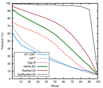
(a)	(b)

Figure 6: Interpolated 11-points precision-recall curves of a selection of visual descriptors for each dataset. (a) LandUse. (b) SatScene.

4.1 Feature evaluation using the basic retrieval scheme

In this section we compare visual descriptors listed in Sec. 3.1 by using the basic retrieval scheme. In order to make the results more concise, in this section we show only the experiments performed employing the Euclidean distance. Given an image dataset, in turn, we used each image as query image and evaluated the results according to the metrics discussed above, i.e. $ANMRR$, $MAP$, $P@5$, $P@10$, $P@50$, $P@100$, $P@1000$ and $EQC$. In the case of the LandUse dataset we performed 2100 queries while in the case of SatScene dataset we evaluated 1005 queries in total.

The results obtained on the LandUse dataset are showed in Table 1, while those obtained on the SatScene dataset are showed in Table 2. Regarding the LandUse dataset, the best results are obtained by using the CNN-based descriptors and in particular the ResNet CNN architectures and the SatResNet-50 that is the fine-tuned ResNet-50. The global hand-crafted descriptors have the lowest performance, with the co-occurrence matrices being the worst one. The local hand-crafted descriptors achieve better results than global hand-crafted descriptors but worse than CNN-based descriptors. In particular, the SatResNet-50, compared with Bag of Dense SIFT and DT-CWT, achieves an $ANMRR$ value that is lower of about 50%, a $MAP$ value that is higher of about 50% , a $P@5$ that is higher of about 50%, a $P@10$ value that is higher of about 50%. The same behavior can be observed for the remaining precision levels. In particular, looking at $P@100$ we can notice that only the SatResNet-50 descriptor is capable of retrieving about 65% of the existing images for each class ($P@100=64.42$). Regarding the SatScene dataset, the best results are obtained by the CNN-based descriptors and in particular the ResNet CNN architectures and the SatResNet-50. The global hand-crafted descriptors have the lowest performance, with the co-occurrence matrices being the worst one. The local hand-crafted descriptors achieve better results than global hand-crafted descriptors but worse than CNN-based descriptors. In particular the SatResNet-50, compared with Bag of Dense SIFT (FV), achieves an $ANMRR$ value that is lower of about 60%, a $MAP$ value that is higher of about 50% , a $P@5$ that is lower of about 20%, a $P@10$ value that is higher of about 30%. Similar behavior can be observed for the remaining precision levels. In particular, looking at $P@50$ we can notice that only SatResNet-50 is capable of retrieving about 70% of the existing images for each class ($P@50=68.02$).

The first columns of tables 6 and 7 show the best performing visual descriptor for each remote sensing image class. For both LandUse and SceneSat datasets, the CNN-based descriptors are the best in the retrieval of all classes. SatResNet-50 performs better than other CNN architectures on most classes apart some classes containing objects rotated and translated on the image plane. In this case, NetVLAD demonstrated to perform better. Looking at Fig. 5 it is interesting to note that NetVLAD, which considers CNN features combined with local features, works better on object-based classes and more important that the SatResNet-50 network clearly outperforms the ResNet-50 thus demonstrating that the domain adaptation of the network to the remote sensing domain helped to handle with the heterogeneous content of remote sensing images.

In Fig. 6 the interpolated 11-points precision-recall curves achieved by a selection of visual descriptors are plotted. It is clear that, in this experiments CNN-based descriptors outperform again other descriptors. It is interesting to note that the SatResNet-50 network clearly outperforms the ResNet-50 thus confirming that the domain adaption has been very effective especially in the case of the SceneSat dataset. This is mostly due to the fact that both the AID and SceneSat datasets are made of pictures taken from Google Earth and then the image content is more similar. In contrast the LandUse dataset is made of picture taken from an aerial device and then the content is quite different in terms of resolution as already discussed in Section  3.3.1.

Concerning the computational cost, the Bag Dense SIFT (FV) is the most costly solution with the worst cost-benefit trade-off. Early after the Bag Dense SIFT (FV), the Vgg M is the other most costly descriptor that is about 200 more costly than the DT-CWT, that is among the global hand-crafted descriptors the best performing one.

One may prefer a less costly retrieval strategy that is less precise and then choose for the DT-CWT. Among the CNN-based descriptors, the Vgg M 128 has better $ANMRR$ values than the DT-CWT for both datasets. The Vgg M 128 is six times more costly than DT-CWT. Concluding, the Vgg M 128 descriptor has the best cost-benefit trade-off.

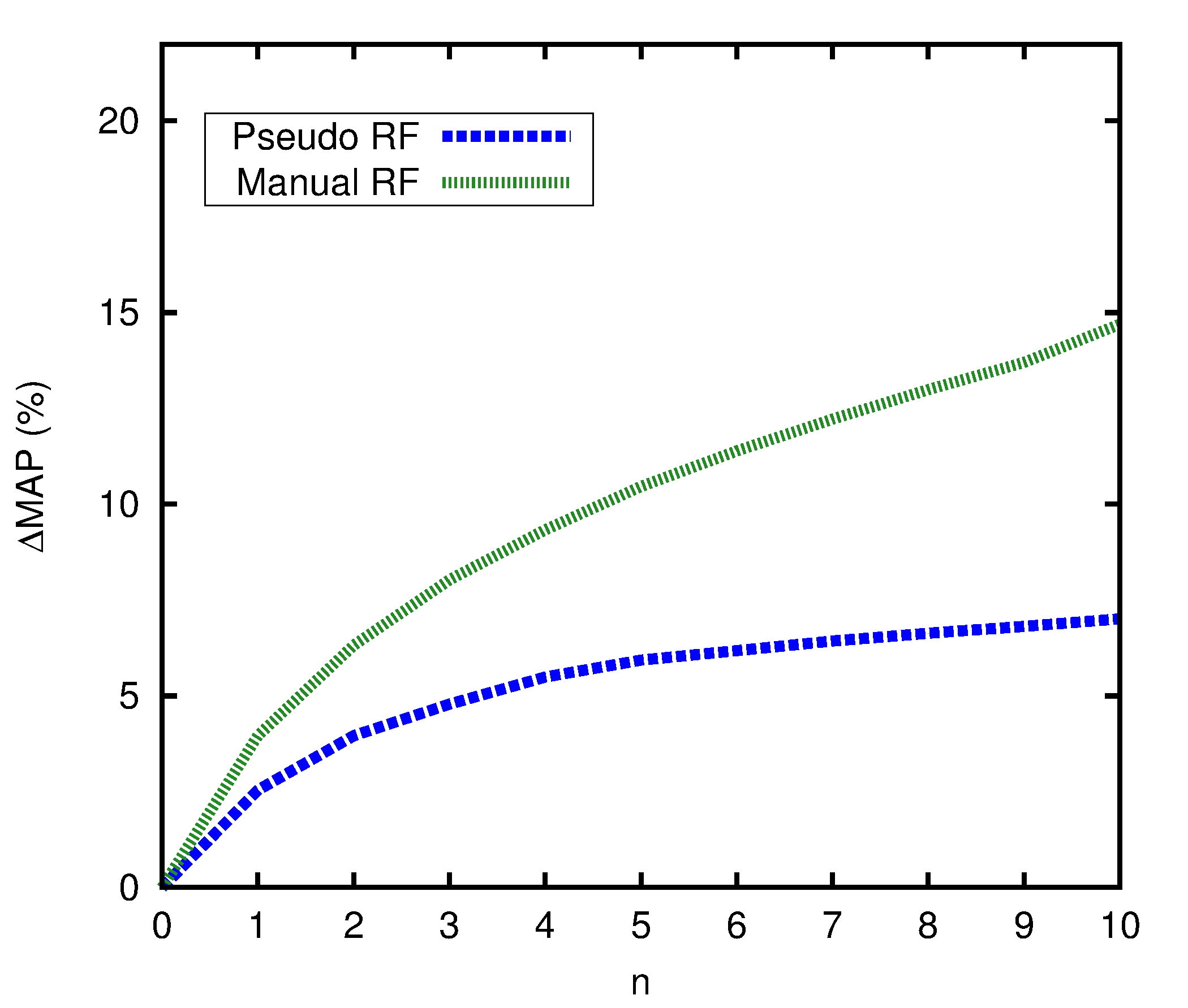
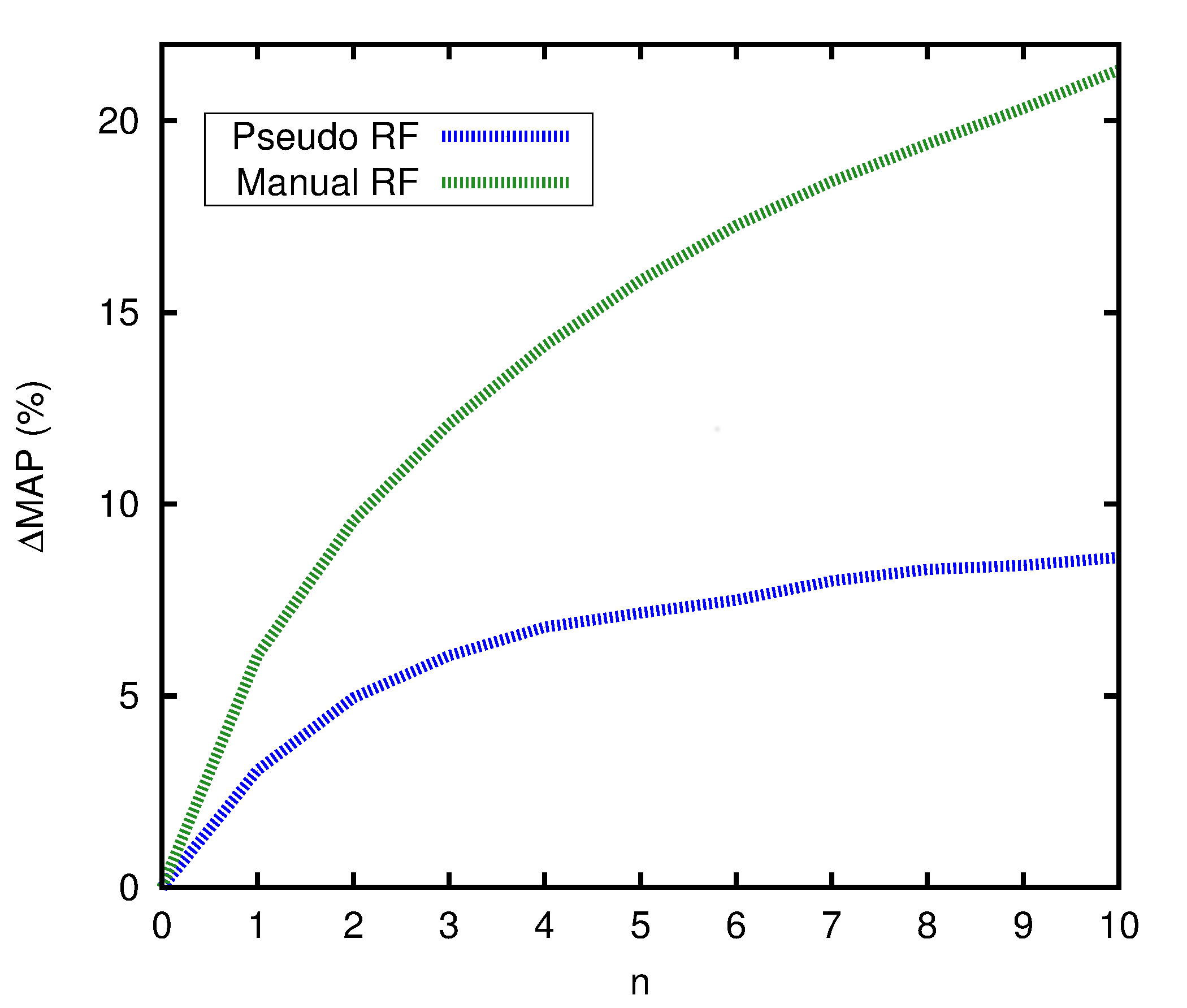
(a)	(b)

Figure 7: Difference of performance ($\Delta MAP$), when the Vgg M is employed, between the pseudo RF and the basic retrieval system, and between manual RF and the basic retrieval system. (a) LandUse. (b) SceneSat.

features	ANMRR	MAP	P@5	P@10	P@50	P@100
Global hand-crafted
Hist. L	0.820	12.31	35.16	28.78	17.42	13.43
Hist. H V	0.783	15.94	53.16	42.82	23.03	16.62
Hist. RGB	0.789	15.37	51.41	41.22	21.89	16.10
Hist. rgb	0.804	14.16	48.09	37.01	20.19	14.93
Spatial Hist. RGB	0.824	13.87	35.15	27.60	16.96	13.27
Co-occ. matr.	0.863	8.56	19.02	16.68	11.88	9.87
CEDD	0.740	19.88	62.27	52.58	29.25	20.55
DT-CWT L	0.708	21.03	39.50	35.67	26.67	22.04
DT-CWT	0.677	24.59	55.13	48.30	32.24	25.00
Gist RGB	0.804	17.14	44.09	35.79	20.46	15.12
Gabor L	0.769	15.92	44.14	36.39	22.16	17.38
Gabor RGB	0.750	18.04	52.56	44.00	25.53	18.97
Opp. Gabor RGB	0.748	18.62	53.73	44.48	25.78	19.32
HoG	0.757	17.79	47.73	40.51	24.69	18.61
Granulometry	0.783	15.26	38.54	31.92	20.29	16.00
LBP L	0.762	16.82	52.23	44.32	26.25	18.61
LBP RGB	0.752	18.06	58.35	49.75	28.16	19.53
Local hand-crafted
Dense LBP RGB	0.747	19.09	59.49	50.99	28.76	20.17
SIFT	0.648	28.56	52.97	47.53	34.65	27.39
Dense SIFT	0.675	25.67	72.20	62.46	35.14	25.75
Dense SIFT (VLAD)	0.652	28.42	74.98	64.82	37.73	27.77
Dense SIFT (FV)	0.652	28.42	74.98	64.82	37.73	27.77
CNN-based
Vgg F	0.360	57.22	85.29	80.91	65.26	52.88
Vgg M	0.344	58.83	86.55	82.73	67.11	54.26
Vgg S	0.350	58.34	86.42	82.58	66.81	53.50
Vgg M 2048	0.348	58.27	85.63	82.21	67.21	53.82
Vgg M 1024	0.358	56.99	85.27	81.79	66.03	52.92
Vgg M 128	0.470	44.46	74.04	69.85	53.60	42.39
BVLC Ref	0.376	55.46	84.84	80.77	63.79	51.34
BVLC AlexNet	0.388	54.31	84.13	79.37	62.18	50.05
Vgg VeryDeep 16	0.365	56.30	84.25	79.88	64.36	52.50
Vgg VeryDeep 19	0.369	55.80	83.42	79.08	63.71	51.99
GoogleNet	0.293	63.89	97.49	90.85	72.81	58.51
ResNet-50	0.305	63.13	98.17	92.54	72.73	57.56
ResNet-101	0.301	63.28	98.43	92.47	72.22	57.83
ResNet-152	0.308	62.58	98.07	91.87	71.14	57.50
NetVLAD	0.324	61.03	97.61	90.30	70.53	56.21
SatResNet-50	0.185	76.55	98.86	95.48	83.79	69.95

(a) LandUse dataset

features	ANMRR	MAP	P@5	P@10	P@50	P@100
Global hand-crafted
Hist. L	0.732	19.73	36.82	31.14	20.49	15.85
Hist. H V	0.713	23.04	42.77	35.80	22.36	16.56
Hist. RGB	0.725	21.34	40.84	33.99	20.85	16.17
Hist. rgb	0.716	22.62	42.73	35.91	22.08	16.43
Spatial Hist. RGB	0.742	21.55	36.92	30.25	19.77	15.14
Co-occ. matr.	0.825	11.57	21.00	17.64	12.72	10.85
CEDD	0.696	23.83	37.71	33.69	23.71	17.77
DT-CWT L	0.677	23.07	35.22	30.87	23.82	19.95
DT-CWT	0.586	33.01	50.65	45.09	32.54	24.23
Gist RGB	0.728	22.66	40.06	34.00	21.40	15.54
Gabor L	0.692	22.38	39.52	33.86	22.84	18.81
Gabor RGB	0.656	26.62	48.60	42.22	26.28	20.37
Opp. Gabor RGB	0.647	27.77	47.54	41.31	27.85	20.52
HoG	0.733	19.81	38.75	34.10	20.96	15.38
Granulometry	0.722	21.07	38.35	32.31	20.19	17.02
LBP L	0.701	22.12	46.43	38.80	23.09	17.50
LBP RGB	0.672	24.70	49.35	42.85	25.62	19.03
Local hand-crafted
Dense LBP RGB	0.669	24.31	50.43	42.40	25.72	19.31
SIFT	0.570	35.64	58.55	51.11	34.25	24.84
Dense SIFT	0.606	31.91	63.50	54.86	31.65	22.11
Dense SIFT (VLAD)	0.554	37.06	70.93	61.99	36.36	24.85
Dense SIFT (FV)	0.523	40.19	71.74	63.37	38.36	27.00
CNN-based
Vgg F	0.372	54.18	72.08	70.39	53.50	34.85
Vgg M	0.383	52.91	72.22	70.31	52.57	34.16
Vgg S	0.381	53.13	72.18	70.45	52.65	34.24
Vgg M 2048	0.386	52.38	71.72	69.83	52.21	34.02
Vgg M 1024	0.398	51.08	70.95	69.12	50.83	33.46
Vgg M 128	0.519	38.16	60.00	56.65	39.14	27.34
BVLC Ref	0.371	54.43	72.00	70.58	53.57	34.88
BVLC AlexNet	0.391	52.44	70.77	68.65	51.56	34.07
Vgg VeryDeep 16	0.402	50.55	71.44	69.18	50.26	33.28
Vgg VeryDeep 19	0.419	48.61	70.01	67.17	48.58	32.48
GoogleNet	0.299	62.12	85.87	81.74	58.14	39.42
ResNet-50	0.231	70.86	92.42	89.15	65.86	42.27
ResNet-101	0.248	68.61	91.88	88.15	63.92	41.50
ResNet-152	0.250	68.50	91.76	87.68	63.90	41.27
NetVLAD	0.332	59.19	86.25	81.34	55.74	37.08
SatResNet-50	0.027	96.14	99.10	98.74	93.25	51.39

(b) SceneSat dataset

Table 3: Results obtained with the Pseudo RF scheme with the Euclidean distance. The lower is the value of $ANMRR$ and $EQC$ the better is the performance. For the other metrics is the opposite. The best result is reported in bold.

features	ANMRR	MAP	P@5	P@10	P@50	P@100
Global hand-crafted
Hist. L	0.798	15.02	71.40	48.34	21.13	15.24
Hist. H V	0.762	18.52	83.90	59.44	26.51	18.39
Hist. RGB	0.771	17.73	80.50	57.16	25.06	17.65
Hist. rgb	0.782	16.73	79.96	54.60	23.80	16.66
Spatial Hist. RGB	0.789	17.47	82.30	52.48	22.59	16.15
Co-occ. matr.	0.853	9.76	38.02	28.78	14.02	10.74
CEDD	0.722	22.23	87.97	66.76	32.28	22.04
DT-CWT L	0.691	23.19	65.54	50.27	29.25	23.32
DT-CWT	0.654	27.21	80.47	62.06	35.64	26.85
Gist RGB	0.767	20.40	84.43	57.66	26.08	18.12
Gabor L	0.754	17.99	71.10	51.05	24.59	18.57
Gabor RGB	0.734	20.11	77.10	56.96	28.26	20.32
Opp. Gabor RGB	0.732	20.80	80.10	58.71	28.55	20.73
HoG	0.733	20.49	78.10	57.23	28.59	20.52
Granulometry	0.770	17.28	67.09	47.36	22.82	17.10
LBP L	0.746	18.91	77.58	57.98	29.05	19.98
LBP RGB	0.737	20.08	82.13	62.40	30.86	20.80
Local hand-crafted
Dense LBP RGB	0.727	21.74	88.73	66.33	32.21	21.76
SIFT	0.602	32.89	88.78	67.16	40.66	31.04
Dense SIFT	0.649	28.38	93.43	75.42	38.82	27.86
Dense SIFT (VLAD)	0.623	31.18	94.79	77.60	41.74	30.13
Dense SIFT (FV)	0.623	31.18	94.79	77.60	41.74	30.13
CNN-based
Vgg F	0.329	60.53	97.39	89.99	69.47	55.64
Vgg M	0.316	61.85	97.82	91.13	70.93	56.64
Vgg S	0.320	61.45	97.58	90.98	70.77	56.04
Vgg M 2048	0.316	61.76	97.97	91.20	71.58	56.66
Vgg M 1024	0.326	60.55	97.78	90.83	70.48	55.73
Vgg M 128	0.422	49.53	95.30	83.89	59.85	46.46
BVLC Ref	0.347	58.63	97.50	89.95	67.71	53.91
BVLC AlexNet	0.357	57.63	97.26	88.90	66.53	52.72
Vgg VeryDeep 16	0.331	60.05	97.24	89.45	68.98	55.48
Vgg VeryDeep 19	0.334	59.56	96.97	88.88	68.39	54.92
GoogleNet	0.257	67.48	86.59	84.09	62.32	41.49
ResNet-50	0.181	77.11	93.53	92.07	71.44	44.65
ResNet-101	0.196	75.13	92.72	90.94	69.40	44.03
ResNet-152	0.203	74.62	92.64	90.63	69.39	43.49
NetVLAD	0.281	66.36	86.35	83.05	61.34	39.60
SatResNet-50	0.014	98.05	99.18	99.31	95.79	51.78

(a) LandUse dataset

features	ANMRR	MAP	P@5	P@10	P@50	P@100
Global hand-crafted
Hist. L	0.698	24.02	67.76	47.75	23.30	17.22
Hist. H V	0.670	28.17	78.95	55.00	25.93	18.30
Hist. RGB	0.686	25.91	72.36	51.58	24.09	17.77
Hist. rgb	0.675	27.44	76.54	54.10	25.35	18.12
Spatial Hist. RGB	0.682	28.06	83.62	54.21	24.86	17.71
Co-occ. matr.	0.803	14.04	41.59	30.37	14.59	11.52
CEDD	0.653	29.59	75.30	54.08	27.26	19.60
DT-CWT L	0.648	26.88	62.55	45.02	26.21	21.13
DT-CWT	0.544	37.90	78.35	59.78	36.08	26.13
Gist RGB	0.660	29.42	83.10	56.85	27.20	18.60
Gabor L	0.663	26.39	68.52	48.85	25.20	19.86
Gabor RGB	0.622	31.02	77.15	57.26	29.28	21.74
Opp. Gabor RGB	0.610	32.29	76.50	57.07	30.94	22.03
HoG	0.688	24.93	72.06	52.61	24.88	17.15
Granulometry	0.701	24.55	67.02	46.41	22.07	17.63
LBP L	0.655	27.47	79.06	56.44	27.07	19.57
LBP RGB	0.628	29.79	78.91	58.92	29.37	20.93
Local hand-crafted
Dense LBP RGB	0.625	29.82	83.16	59.42	29.55	21.11
SIFT	0.508	42.25	89.27	68.54	39.56	27.79
Dense SIFT	0.554	37.83	90.55	71.12	36.35	24.38
Dense SIFT (VLAD)	0.493	43.48	94.37	77.44	41.69	27.70
Dense SIFT (FV)	0.493	43.48	94.37	77.44	41.69	27.70
CNN-based
Vgg F	0.330	59.44	92.22	80.82	57.44	36.75
Vgg M	0.340	58.30	92.36	81.06	56.41	36.10
Vgg S	0.336	58.69	92.42	81.15	56.74	36.34
Vgg M 2048	0.339	58.46	92.78	81.52	56.65	36.12
Vgg M 1024	0.349	57.21	92.78	80.85	55.31	35.73
Vgg M 128	0.448	46.57	90.89	74.01	45.39	30.70
BVLC Ref	0.327	59.89	92.38	81.55	57.63	36.80
BVLC AlexNet	0.343	58.26	92.72	80.74	55.97	36.16
Vgg VeryDeep 16	0.359	55.99	92.12	79.91	54.07	35.24
Vgg VeryDeep 19	0.368	54.79	91.84	79.23	53.23	34.76
GoogleNet	0.215	72.83	98.29	93.00	66.40	43.43
ResNet-50	0.153	80.54	99.76	97.28	74.27	45.92
ResNet-101	0.168	78.56	99.46	96.14	72.24	45.35
ResNet-152	0.173	78.30	99.62	96.43	72.43	44.82
NetVLAD	0.229	72.29	98.87	94.09	66.35	41.97
SatResNet-50	0.009	98.69	100.00	99.99	96.46	51.95

(b) SceneSat dataset

Table 4: Results obtained with the Manual RF scheme with the Euclidean distance. The lower is the value of $ANMRR$ and $EQC$ the better is the performance. For the other metrics is the opposite. For each row the best result is reported in bold.

4.2 Feature evaluation using the pseudo-RF retrieval scheme

In the case of pseudo RF, we used the top $n$ images retrieved after the initial query for re-querying the system. The computational cost of such a system is $n$ times higher than the cost of a basic system.

Results obtained choosing $n=5$ are showed in Table 3(a) and  3(b) for the LandUse and SatScene datasets respectively. It can be noticed that, in both cases, the employment of the pseudo RF scheme gives an improvement with respect to the basic retrieval system whatever is the visual descriptor employed. The CNN-based and local hand-crafted descriptors that, when used in a basic system, obtained the highest precision at level 5 ($Pr@5$), have the largest improvement of performance.

Figures 7(a) and (b) show the difference of MAP between the pseudo RF scheme and the basic retrieval scheme, when the Vgg visual descriptor is employed. The value $n$ ranges from 0 (that corresponds to the basic system) to 10. It can be noticed that the improvement of performance, when $n$ is equal to 5, is of about $5\%$ in the case of LandUse and of about $7\%$ in the case of SceneSat dataset.

The second columns of tables 6 and 7 show the best performing visual descriptor for each remote sensing image class. In both cases, LandUse and SceneSat, the best performing visual descriptors are quite the same as in the case of the basic retrieval system.

4.3 Feature evaluation using the manual-RF retrieval scheme

In manual RF, we used the first $n$ actually relevant images retrieved after the initial query for re-querying the system. The computational cost of such a system is $n$ times higher than the cost of a basic system. The first five relevant images appear, in the worst case (co-occurrence matrix), within the top 50 images, while in the best case (SatResNet-50), within the top 6 or 7 images (cfr. table 1).

Results obtained choosing $n=5$ are showed in Table 4(a) and  4(b) for the LandUse and SatScene datasets respectively. It can be noticed that, in both cases, the employment of the manual RF scheme gives an improvement with respect to both the basic retrieval and the pseudo RF systems. The CNN-based and local hand-crafted descriptors that, when used in a basic system, obtained the highest precision at level 5 ($Pr@5$), have also in this case the largest improvement of performance.

Figures 7(a) and (b) show the difference between the MAP of the manual RF scheme and the basic retrieval scheme, when the Vgg visual descriptor is employed, The value $n$ ranges from 0 (that corresponds to the basic system) to 10. It can be noticed that for both datasets the improvement of performance is, when $n$ is equal to 5, of about $9\%$ in the case of LandUse and of about $14\%$ in the case of SceneSat. The manual RF scheme, when $n$ is equal to 1, achieves the same performance of the pseudo RF when $n$ is equal to 2.

The third columns of tables 6 and 7 show the best performing visual descriptor for each remote sensing image class. In both cases, LandUse and SceneSat, the best performing visual descriptors are quite the same as in the cases of the basic and pseudo-RF retrieval system.

4.4 Feature evaluation using the active-learning-based-RF retrieval scheme

We considered the Active-Learning-based RF scheme as presented by Demir et al. Demir and Bruzzone (2015). As suggested by the original authors, we considered the following parameters: 10 RF iterations; an initial training set made of 2 relevant and 3 not relevant images; $p=20$ ambiguous images; $h=5$ diverse images; the histogram intersection as measure of similarity between feature vectors. The histogram intersection distance is defined as follows:

$$HI(\mathbf{x},\mathbf{y})=\sum_{l=1}^{L}min(x_{l},y_{l}),$$

where $\mathbf{x}$ and $\mathbf{y}$ are the feature vectors of two generic images and $L$ is the size of the feature vector.

Results are showed in Table 5(a) and  5(b) for the LandUse and SatScene datasets respectively. Regarding the LandUse dataset, it can be noticed that the employment of this RF scheme gives an improvement with respect to the other retrieval schemes for all the visual descriptors. In the case of CNN-based descriptors the improvement is of about 20%. Surprisingly, in the case of SceneSat dataset, the employment of the Active-Learning-based RF scheme gives a performance improvement only in the cases of hand-crafted descriptors and most recent CNN architectures like ResNet or NetVLAD. In the best case, that is NetVLAD, the improvement is of about 80%. It is very interesting to note that for both datasets, the best performing descriptor is the NetVLAD. This is mostly due to the fact that this feature vector compared with the others extracted from different CNN architecture is less sparse. The degree of sparseness of feature vectors makes the Support Vector Machine, that is employed in the case of Active-Learning-based RF scheme, less or more effective.

The fourth columns of tables 6 and 7 show the best performing visual descriptor for each remote sensing image class. In the case of LandUse dataset, the best performing visual descriptors are the CNN-based descriptors, while in the case of SceneSat dataset, the best performing are the local hand-crafted descriptors apart from a few number of classes.

features	ANMRR	MAP	P@5	P@10	P@50	P@100
Global hand-crafted
Hist. L	0.753	19.18	71.46	52.51	25.23	18.82
Hist. H V	0.688	25.57	87.31	70.88	34.65	24.31
Hist. RGB	0.747	20.12	80.07	61.73	27.77	19.50
Hist. rgb	0.712	23.25	83.35	63.96	30.50	22.22
Spatial Hist. RGB	0.695	25.27	84.49	64.50	32.39	23.52
Coocc. matr.	0.851	10.28	32.18	24.41	13.94	10.94
CEDD	0.719	22.72	85.49	68.70	32.43	21.94
DT-CWT L	0.757	18.78	56.10	42.78	24.67	18.81
DT-CWT	0.698	24.48	77.90	63.52	33.58	23.73
Gist RGB	0.662	27.76	87.06	70.17	37.91	27.11
Gabor L	0.748	19.19	61.67	44.56	23.95	18.61
Gabor RGB	0.709	23.43	69.60	53.30	30.05	22.74
Opp. Gabor RGB	0.634	29.78	82.34	66.71	39.40	29.42
HoG	0.681	26.18	84.70	68.10	36.06	25.20
Granulometry	0.833	14.39	54.11	36.23	16.92	12.76
LBP L	0.791	16.82	64.78	47.73	24.17	16.49
LBP RGB	0.793	16.77	69.43	51.66	24.26	16.41
Local hand-crafted
Dense LBP RGB	0.726	22.41	85.21	68.24	31.99	21.34
SIFT	0.572	35.40	80.31	65.13	44.08	34.64
Dense SIFT	0.631	32.09	90.27	76.93	41.81	29.82
Dense SIFT (VLAD)	0.598	34.39	88.87	76.44	43.70	31.92
Dense SIFT (FV)	0.465	48.38	98.58	92.97	61.48	44.70
CNN-based
Vgg F	0.256	69.33	99.70	97.47	79.92	63.90
Vgg M	0.247	71.09	99.39	98.09	82.98	65.54
Vgg S	0.260	69.45	99.34	96.42	79.88	63.61
Vgg M 2048	0.248	70.54	98.51	96.27	80.43	65.05
Vgg M 1024	0.266	68.22	99.09	96.84	78.75	62.73
Vgg M 128	0.333	60.72	97.70	94.03	73.60	56.17
BVLC Ref	0.292	66.05	98.70	95.98	76.56	60.72
BVLC AlexNet	0.281	66.98	99.49	96.77	77.36	61.58
Vgg VeryDeep 16	0.292	66.05	98.70	95.98	76.56	60.72
Vgg VeryDeep 19	0.292	66.05	98.70	95.98	76.56	60.72
GoogleNet	0.209	75.41	99.76	98.84	87.09	69.36
ResNet-50	0.332	63.34	99.45	98.01	77.00	56.72
ResNet-101	0.311	65.42	99.59	98.33	79.15	58.97
ResNet-152	0.318	64.74	99.68	98.38	78.71	57.81
NetVLAD	0.144	82.43	99.80	99.32	91.31	76.35
SatResNet-50	0.232	74.40	99.46	98.89	87.44	67.66

(a) LandUse dataset

features	ANMRR	MAP	P@5	P@10	P@50	P@100
Global hand-crafted
Hist. L	0.648	28.93	67.96	52.19	27.10	20.01
Hist. H V	0.574	36.02	76.44	61.02	34.64	23.78
Hist. RGB	0.646	29.86	74.03	57.51	28.50	19.43
Hist. rgb	0.587	35.72	76.70	62.33	33.68	22.71
Spatial Hist. RGB	0.549	38.34	80.78	64.05	36.62	25.10
Coocc. matr.	0.804	14.72	42.03	31.14	14.93	11.25
CEDD	0.673	27.15	69.53	53.37	26.10	18.20
DT-CWT L	0.688	25.51	55.14	42.37	23.85	18.12
DT-CWT	0.571	37.60	71.54	57.35	35.32	23.91
Gist RGB	0.551	38.50	88.12	70.45	36.75	24.55
Gabor L	0.672	26.71	65.65	46.94	24.21	19.31
Gabor RGB	0.612	32.21	70.51	55.46	30.40	22.13
Opp. Gabor RGB	0.473	46.13	86.77	74.32	44.11	29.00
HoG	0.699	24.17	73.53	53.95	23.91	16.37
Granulometry	0.794	18.23	53.31	37.13	15.88	11.59
LBP L	0.669	26.62	72.44	54.86	26.68	18.24
LBP RGB	0.667	27.26	65.65	49.47	26.07	19.14
Local hand-crafted
Dense LBP RGB	0.534	39.84	84.20	68.96	37.18	26.25
SIFT	0.473	46.13	89.61	76.34	43.64	29.25
Dense SIFT	0.455	48.71	92.30	80.85	45.83	29.47
Dense SIFT (VLAD)	0.396	54.98	91.98	84.73	50.72	33.14
Dense SIFT (FV)	0.301	65.81	97.31	94.01	60.48	37.57
CNN-based
Vgg F	0.520	44.87	83.66	68.39	41.36	25.67
Vgg M	0.503	46.40	84.82	70.47	42.82	26.35
Vgg M 128	0.558	39.27	81.57	67.82	37.05	23.81
Vgg S	0.479	48.61	84.90	72.35	44.81	27.90
Vgg M 2048	0.467	48.85	84.60	72.33	46.05	28.59
Vgg M 1024	0.468	48.55	85.57	72.21	45.58	28.61
BVLC Ref	0.522	44.41	82.75	68.66	41.30	25.38
BVLC AlexNet	0.506	46.57	82.67	69.22	42.32	26.41
Vgg VeryDeep 16	0.505	46.77	86.97	72.49	42.40	26.27
Vgg VeryDeep 19	0.498	46.83	82.53	70.32	43.55	26.59
GoogleNet	0.112	86.56	99.84	99.34	81.44	46.96
ResNet-50	0.152	82.46	99.96	99.82	76.96	44.73
ResNet-101	0.162	81.52	99.96	99.64	75.86	44.16
ResNet-152	0.161	81.46	99.94	99.62	75.80	44.26
NetVLAD	0.048	93.89	100.00	99.94	89.11	50.28
SatResNet-50	0.054	94.20	99.98	99.98	91.42	49.29

(b) SceneSat dataset

Table 5: Results obtained with the Active-Learning-based RF scheme. The lower is the value of $ANMRR$ and $EQC$ the better is the performance. For the other metrics is the opposite. For each row the best result is reported in bold.

categories	image	basic IR	pseudo RF	manual RF	act. learn. RF
agricultural		Vgg M	ResNet-101	Vgg VeryDeep 19	NetVLAD
		(0.092)	(0.065)	(0.048)	(0.011)
airplane		SatResNet-50	SatResNet-50	SatResNet-50	NetVLAD
		(0.148)	(0.103)	(0.084)	(0.033)
baseballdiamond		SatResNet-50	SatResNet-50	SatResNet-50	BVLC Ref
		(0.109)	(0.060)	(0.059)	(0.076)
beach		SatResNet-50	SatResNet-50	SatResNet-50	Vgg F
		(0.031)	(0.021)	(0.021)	(0.006)
buildings		SatResNet-50	SatResNet-50	SatResNet-50	SatResNet-50
		(0.412)	(0.368)	(0.302)	(0.271)
chaparral		NetVLAD	NetVLAD	NetVLAD	NetVLAD
		(0.007)	(0.003)	(0.003)	(0.001)
denseresidential		SatResNet-50	SatResNet-50	SatResNet-50	NetVLAD
		(0.564)	(0.561)	(0.521)	(0.444)
forest		SatResNet-50	Vgg M	Vgg M	NetVLAD
		(0.035)	(0.023)	(0.021)	(0.008)
freeway		SatResNet-50	SatResNet-50	SatResNet-50	NetVLAD
		(0.280)	(0.260)	(0.256)	(0.142)
golfcourse		SatResNet-50	SatResNet-50	SatResNet-50	NetVLAD
		(0.232)	(0.181)	(0.169)	(0.092)
harbor		NetVLAD	NetVLAD	NetVLAD	NetVLAD
		(0.069)	(0.051)	(0.051)	(0.001)
intersection		SatResNet-50	SatResNet-50	SatResNet-50	SatResNet-50
		(0.356)	(0.289)	(0.262)	(0.212)
mediumresidential		SatResNet-50	SatResNet-50	SatResNet-50	NetVLAD
		(0.390)	(0.360)	(0.337)	(0.292)
mobilehomepark		SatResNet-50	SatResNet-50	SatResNet-50	NetVLAD
		(0.329)	(0.304)	(0.278)	(0.155)
overpass		SatResNet-50	SatResNet-50	SatResNet-50	NetVLAD
		(0.190)	(0.152)	(0.130)	(0.150)
parkinglot		SatResNet-50	SatResNet-50	SatResNet-50	Vgg F
		(0.002)	(0.001)	(0.001)	(0.006)
river		SatResNet-50	SatResNet-50	SatResNet-50	NetVLAD
		(0.365)	(0.317)	(0.283)	(0.196)
runway		GoogleNet	GoogleNet	GoogleNet	NetVLAD
		(0.256)	(0.194)	(0.191)	(0.061)
sparseresidential		SatResNet-50	SatResNet-50	SatResNet-50	GoogleNet
		(0.194)	(0.127)	(0.105)	(0.123)
storagetanks		SatResNet-50	SatResNet-50	SatResNet-50	NetVLAD
		(0.363)	(0.331)	(0.278)	(0.176)
tenniscourt		SatResNet-50	SatResNet-50	SatResNet-50	GoogleNet
		(0.402)	(0.360)	(0.275)	(0.216)

Table 6: LandUse dataset: ANMRR evaluation across retrieval schemes and RS image classes . For each class and retrieval scheme is reported the best visual descriptor. Orange color stands for fine-tuned CNN-based descriptors, blue color stands for pre-trained CNN-based descriptors, yellow color stands for NetVLAD-based descriptors while cyan color stands for global hand-crafted descriptors.

categories	image	basic IR	pseudo RF	manual RF	act. learn. RF
Airport		SatResNet-50	SatResNet-50	SatResNet-50	NetVLAD
		(0.049)	(0.015)	(0.008)	(0.015)
Beach		SatResNet-50	SatResNet-50	Vgg M	SatResNet-50
		(0.046)	(0.040)	(0.037)	(0.004)
Bridge		SatResNet-50	SatResNet-50	SatResNet-50	GoogleNet
		(0.021)	(0.001)	(0.001)	(0.048)
Commercial		SatResNet-50	SatResNet-50	SatResNet-50	SatResNet-50
		(0.027)	(0.008)	(0.005)	(0.084)
Desert		SatResNet-50	SatResNet-50	SatResNet-50	Opp. Gabor RGB
		(0.005)	(0.003)	(0.003)	(0.004)
Farmland		SatResNet-50	SatResNet-50	SatResNet-50	NetVLAD
		(0.054)	(0.034)	(0.013)	(0.027)
footballField		SatResNet-50	SatResNet-50	SatResNet-50	SatResNet-50
		(0.001)	(0.001)	(0.001)	(0.001)
Forest		SatResNet-50	SatResNet-50	SatResNet-50	NetVLAD
		(0.017)	(0.014)	(0.005)	(0.033)
Industrial		SatResNet-50	SatResNet-50	SatResNet-50	SatResNet-50
		(0.073)	(0.050)	(0.028)	(0.145)
Meadow		SatResNet-50	SatResNet-50	SatResNet-50	NetVLAD
		(0.020)	(0.008)	(0.006)	(0.035)
Mountain		SatResNet-50	SatResNet-50	SatResNet-50	NetVLAD
		(0.014)	(0.005)	(0.005)	(0.003)
Park		SatResNet-50	SatResNet-50	SatResNet-50	SatResNet-50
		(0.030)	(0.014)	(0.008)	(0.012)
Parking		SatResNet-50	SatResNet-50	SatResNet-50	NetVLAD
		(0.003)	(0.001)	(0.001)	(0.010)
Pond		SatResNet-50	SatResNet-50	SatResNet-50	SatResNet-50
		(0.014)	(0.004)	(0.003)	(0.030)
Port		SatResNet-50	SatResNet-50	SatResNet-50	NetVLAD
		(0.048)	(0.016)	(0.010)	(0.058)
railwayStation		SatResNet-50	SatResNet-50	SatResNet-50	SatResNet-50
		(0.016)	(0.021)	(0.004)	(0.031)
Residential		SatResNet-50	SatResNet-50	SatResNet-50	NetVLAD
		(0.075)	(0.034)	(0.031)	(0.033)
River		SatResNet-50	SatResNet-50	SatResNet-50	SatResNet-50
		(0.001)	(0.001)	(0.001)	(0.005)
Viaduct		SatResNet-50	SatResNet-50	SatResNet-50	NetVLAD
		(0.001)	(0.001)	(0.001)	(0.005)

Table 7: LandUse dataset: ANMRR evaluation across retrieval schemes and RS image classes . For each class and retrieval scheme is reported the best visual descriptor. Orange color stands for fine-tuned CNN-based descriptors, blue color stands for pre-trained CNN-based descriptors, yellow color stands for NetVLAD-based descriptors while cyan color stands for global hand-crafted descriptors.

	basic IR		pseudo RF		manual RF		act. learn. RF		Overall
features	ANMRR	EQC	ANMRR	EQC	ANMRR	EQC	ANMRR	EQC	avg rank
SatResNet-50	0.133	409	0.110	2045	0.097	2045	0.143	8180	5.08
GoogleNet	0.329	204	0.290	1020	0.254	1020	0.160	4080	5.49
ResNet-50	0.294	409	0.255	2045	0.229	2045	0.241	8180	5.72
ResNet-101	0.302	409	0.261	2045	0.234	2045	0.236	8180	5.92
ResNet-152	0.305	409	0.267	2045	0.240	2045	0.238	8180	6.59
Vgg M 2048	0.410	409	0.367	2045	0.327	2045	0.375	8180	8.87
NetVLAD	0.369	819	0.326	4095	0.277	4095	0.096	16380	9.02
Vgg M 1024	0.422	204	0.378	1020	0.337	1020	0.380	4080	9.19
Vgg M	0.398	819	0.363	4095	0.328	4095	0.386	16380	9.45
Vgg S	0.398	819	0.365	4095	0.328	4095	0.371	16380	9.55
Vgg F	0.397	819	0.366	4095	0.329	4095	0.398	16380	9.90
Vgg M 128	0.525	25	0.494	125	0.435	125	0.463	500	10.81
BVLC Ref	0.404	819	0.374	4095	0.337	4095	0.409	16380	11.18
DT-CWT	0.628	4	0.632	20	0.599	20	0.634	80	11.22
Vgg VeryDeep 19	0.427	819	0.394	4095	0.351	4095	0.307	16380	11.81
Vgg VeryDeep 16	0.416	819	0.383	4095	0.345	4095	0.403	16380	12.02
BVLC AlexNet	0.416	819	0.389	4095	0.350	4095	0.403	16380	12.03
SIFT	0.597	204	0.609	1020	0.555	1020	0.522	4080	12.45
Dense SIFT	0.638	204	0.641	1020	0.602	1020	0.543	4080	12.61
Opp. Gabor RGB	0.692	52	0.698	260	0.671	260	0.553	1040	13.56
DT-CWT L	0.690	1	0.693	5	0.670	5	0.655	20	13.74
Dense SIFT (FV)	0.579	8192	0.582	40960	0.535	40960	0.498	163840	13.82
Dense SIFT (VLAD)	0.601	5120	0.603	25600	0.559	25600	0.384	102400	13.93
Dense LBP RGB	0.702	204	0.708	1020	0.676	1020	0.631	4080	14.10
Gabor RGB	0.699	19	0.703	95	0.678	95	0.659	380	14.27
LBP RGB	0.708	10	0.713	50	0.683	50	0.730	200	14.82
CEDD	0.710	28	0.718	140	0.687	140	0.696	560	14.95
Hist. H V	0.741	102	0.747	510	0.715	510	0.630	2040	15.55
Gabor L	0.726	6	0.731	30	0.709	30	0.709	120	15.76
LBP L	0.725	48	0.732	240	0.701	240	0.729	960	16.01
Gist RGB	0.743	102	0.765	510	0.713	510	0.606	2040	16.53
HoG	0.737	16	0.744	80	0.710	80	0.688	320	16.91
Hist. rgb	0.750	153	0.759	765	0.728	765	0.648	3060	17.18
Granulometry	0.748	15	0.752	75	0.735	75	0.813	300	17.39
Hist. L	0.772	51	0.776	255	0.748	255	0.661	1020	18.11
Hist. RGB	0.754	153	0.757	765	0.728	765	0.695	3060	18.35
Spatial Hist. RGB	0.763	307	0.783	1535	0.735	1535	0.621	6140	18.67
Coocc. matr.	0.841	1	0.844	5	0.828	5	0.827	20	19.08

Table 8: Average rank across datasets of each visual descriptor performance. The list of visual descriptors reported in the table is ordered by the average rank (last column of the table) that is obtained by averaging the ranks achieved by each visual descriptor across datasets, retrieval schemes and measures: $ANMRR$, $MAP$, $Pr$ at 5,10,50,100 levels, and EQC. For sake of completeness, for each retrieval scheme, the table shows the average ANMRR across datasets and the EQC for each visual descriptor. For each retrieval scheme, the best average ANMRR performance is reported in bold.

4.5 Average rank of visual descriptors across RS datasets

In table 8 we show the average rank of all the visual descriptors evaluated. The average rank is represented in the last column and obtained by averaging the ranks achieved by each visual descriptor across datasets, retrieval schemes and measures: $ANMRR$, $MAP$, $Pr$ at 5,10,50,100 levels, and EQC. For sake of completeness, for each retrieval scheme, we displayed the average ANMRR across datasets and the EQC for each visual descriptor. From this table is quite clear that across datasets, the best performing visual descriptors are the CNN-based ones. The first 13 positions out of 38 are occupied by CNN-based descriptors. The global hand-crafted descriptor DT-CWT is at 14th position mostly because of the length of the vector that is very short. After some other CNN-based descriptors, we find the local hand-crafted descriptors that despite their good performance, they are penalized by the size of the vector of feature that is very long, in the case of Dense SIFT (FV) is 40960 that is 2048 times higher than the size of DT-CWT.

Looking at the EQC columns of each retrieval schemes of table 8, it is quite evident that the use of Active-Learning-based RF is not always convenient. For instance, in the case of the top 5 visual descriptors of the table, the Active-Learning-based RF achieves globally worse performance than pseudo-RF with a much more higher EQC. This is not true in all other cases, where the performance achieved with the Active-Learning-based RF is better than pseudo-RF.

Notwithstanding this, the employment of techniques to speed-up the nearest image search process makes the AL-RF scheme not as computationally expensive as argued in the previous paragraph. Large amount of data and high dimensional feature vector, makes the nearest image search process very slow. The main bottleneck of the search is the access to the memory. The employment of a compact representation of the feature vectors, such as hash Zhao et al. (2015) or polysemous codes Douze, Jégou, and Perronnin (2016), is likely to offer a better efficiency than the use of full vectors thus accelerating the image search process. Readers who would wish to deepen the subject can refer to the following papers Zhao et al. (2015); Lu, Liong, and Zhou (2017); Douze, Jégou, and Perronnin (2016); Zhao et al. (2015).

4.6 Comparison with the state of the art

According to our results, one of the best performing visual descriptor is the ResNet and in particular SatResNet-50, while the best visual descriptor, when the computational cost is taken into account, is the Vgg M 128. We compared these descriptors, coupled with the four scheme described in Sec. 3.2, with some recent methods Bosilj et al. (2016); Aptoula (2014); Ozkan et al. (2014); Yang and Newsam (2013). All these works used the basic retrieval scheme and the experiments have been conducted on the LandUse dataset. Aptoula proposed several global morphological texture descriptors Bosilj et al. (2016); Aptoula (2014). Ozkan et al. used bag of visual words (BoVW) descriptors, the vector of locally aggregated descriptors (VLAD) and the quantized VLAD (VLAD-PQ) descriptors Ozkan et al. (2014). Yang et al. Yang and Newsam (2013) investigated the effects of a number of design parameters on the BoVW representation. They considered: saliency-versus grid-based local feature extraction, the size of the visual codebook, the clustering algorithm used to create the codebook, and the dissimilarity measure used to compare the BOVW representations.

The results of the comparison are shown in Table 9. The Bag of Dense SIFT (VLAD) presented in Ozkan et al. (2014) achieves performance that is close to the CNN-based descriptors. This method achieves $ANMRR=0.460$ with $EQC=5120$. This result has been obtained considering a codebook built by using images from the LandUse dataset. Concerning the computational cost, the texture features Yang and Newsam (2013); Aptoula (2014) are better than SatResNet-50 and Vgg M 128. In terms of trade-off between performance and computational cost, the Vgg M 128 descriptor achieves a $ANMRR$ value that is about 25% lower than the one achieved by the CCH+RIT+FPS₁+FPS₂ descriptor used in Aptoula (2014) with a computational cost that is about 2 times higher.

features	Hist. Inters.	Euclidean	Cosine	Manhattan	$\chi^{2}$-square	Length	Time (sec)	EQC
CCH RIT FPS1 FPS2 Aptoula (2014)	0.609	0.640	-	0.589	0.575	62	-	12
CCH Aptoula (2014)	0.677	0.726	-	0.677	0.649	20	1.9	4
RIT Aptoula (2014)	0.751	0.769	-	0.751	0.757	20	2.3	4
FPS1 Aptoula (2014)	0.798	0.731	-	0.740	0.726	14	1.6	2
FPS2 Aptoula (2014)	0.853	0.805	-	0.790	0.783	8	1.6	1
pLPS-aug Bosilj et al. (2016)	-	0.472	-	-	-	12288	-	2458
Texture Yang and Newsam (2013)	-	0.630	-	-	-	-	40.4	-
Local features Yang and Newsam (2013)		0.591	-	-	-	-	193.3	-
Dense SIFT (BoVW) Ozkan et al. (2014)	-	-	0.540	-	-	1024	9.4	204
Dense SIFT (VLAD) Ozkan et al. (2014)	-	-	0.460	-	-	25600	129.3	5120
B-IR Vgg M 128	0.544	0.488	0.488	0.493	0.488	128	-	25
B-IR ResNet-50	0.476	0.358	0.358	0.395	0.350	2048	-	409
B-IR SatResNet-50	0.331	0.239	0.239	0.271	0.233	2048	-	409
P-RF Vgg M 128	0.550	0.470	0.470	0.466	0.458	128	-	125
P-RF ResNet-50	0.493	0.305	0.305	0.390	0.324	2048	-	2045
P-RF SatResNet-50	0.332	0.185	0.185	0.250	0.200	2048	-	2045
M-RF Vgg M 128	0.497	0.422	0.422	0.416	0.410	128	-	125
M-RF ResNet-50	0.459	0.181	0.181	0.359	0.299	2048	-	2045
M-RF SatResNet-50	0.307	0.014	0.014	0.224	0.179	2048	-	2045
AL-RF Vgg M 128	0.333	-	-	-	-	128	-	500
AL-RF ResNet-50	0.332	-	-	-	-	2048	-	8180
AL-RF SatResNet-50	0.232	-	-	-	-	2048	-	8180

Table 9: ANMRR comparison on the LandUse dataset. The lower is the result, the better is the performance. For each column the best result is reported in bold.

5 Conclusions

In this work we presented an extensive evaluation of visual descriptors for content-based retrieval of remote sensing images. We evaluated global hand-crafted, local hand-crafted and Convolutional Neural Networks features coupled with four different content-based retrieval (CBIR) schemes: a basic CBIR, a pseudo relevance feedback (RF), a manual RF and an active-learning-based RF. The experimentation has been conducted on two publicly available datasets that are different in terms of image size and resolution. Results demonstrated that:

• CNN-based descriptors proved to perform better, on average, than both global hand-crafted and local hand-crafted descriptors whatever is the retrieval scheme adopted and on both the datasets considered, see the summary table 8;

• The RS domain adaptation of the ResNet-50 has led to a notable improvement of performance with respect to CNNs pre-trained on multimedia scene and object images. This demonstrated the importance of domain adaptation in the field of remote sensing images;

• NetVLAD works better on those images that contain fine-grained textures and objects. NetVLAD is a CNN that considers local features. This is true specially for the LandUse dataset on classes like: chaparral, harbor, runaway, etc. See the tables 6 and 7 and figures 5;

• Pseudo and manual relevance feedback schemes demonstrated to be very effective only when coupled with a visual descriptor that is high performing in a basic retrieval system, such as CNN-based and local hand-crafted descriptors. This is quite evident looking at 7a and b;

• Active-Learning-based RF demonstrated to be very effective on average and the best performing among retrieval schemes. The computational cost required to perform one query is, on average, at least 4 times higher than the computational cost required to perform a query with the other considered RF schemes and at least 20 times higher than a basic retrieval scheme.

As future works, it would be interesting to experiments the efficiency of techniques to speed up the image search process by exploiting compact feature vector representations such as has, or polysemous codes.

Competing interests

The author declare that he has no competing interests.

Funding

We gratefully acknowledge the support of NVIDIA Corporation with the donation of the Tesla K40 GPU used for doing part of the experiments included in this research.

References

- Aptoula (2014) Aptoula, Erchan. 2014. “Remote sensing image retrieval with global morphological texture descriptors.” Geoscience and Remote Sensing, IEEE Transactions on 52 (5): 3023–3034.
- Arandjelovic et al. (2016) Arandjelovic, Relja, Petr Gronat, Akihiko Torii, Tomas Pajdla, and Josef Sivic. 2016. “NetVLAD: CNN architecture for weakly supervised place recognition.” In Proceedings of the IEEE Conference on Computer Vision and Pattern Recognition, 5297–5307.
- Arvis et al. (2004) Arvis, Vincent, Christophe Debain, Michel Berducat, and Albert Benassi. 2004. “Generalization of the cooccurrence matrix for colour images: Application to colour texture.” Image Analysis & Stereology 23 (1).
- Baeza-Yates, Ribeiro-Neto et al. (1999) Baeza-Yates, Ricardo, Berthier Ribeiro-Neto, et al. 1999. Modern information retrieval. Vol. 463. ACM press New York.
- Barilla and Spann (2008) Barilla, M.E., and M. Spann. 2008. “Colour-based texture image classification using the complex wavelet transform.” In Electrical Engineering, Computing Science and Automatic Control, 2008. CCE 2008. 5th International Conference on, nov., 358 –363.
- Bianco et al. (2015) Bianco, S, D Mazzini, DP Pau, and R Schettini. 2015. “Local detectors and compact descriptors for visual search: A quantitative comparison.” Digital Signal Processing 44: 1–13.
- Bianconi and Fernández (2007) Bianconi, F, and A. Fernández. 2007. “Evaluation of the effects of Gabor filter parameters on texture classification.” Pattern Recognition 40 (12): 3325 – 3335.
- Bianconi et al. (2011) Bianconi, F., R. Harvey, P. Southam, and A. Fernández. 2011. “Theoretical and experimental comparison of different approaches for color texture classification.” Journal of Electronic Imaging 20 (4).
- Bosilj et al. (2016) Bosilj, Petra, Erchan Aptoula, Sébastien Lefèvre, and Ewa Kijak. 2016. “Retrieval of Remote Sensing Images with Pattern Spectra Descriptors.” ISPRS International Journal of Geo-Information 5 (12): 228.
- Brinke, Squire, and Bigelow (2004) Brinke, Walter, David McG Squire, and John Bigelow. 2004. “Similarity: measurement, ordering and betweenness.” In Knowledge-Based Intelligent Information and Engineering Systems, 996–1002. Springer.
- Chatfield et al. (2014) Chatfield, Ken, Karen Simonyan, Andrea Vedaldi, and Andrew Zisserman. 2014. “Return of the devil in the details: Delving deep into convolutional nets.” arXiv preprint arXiv:1405.3531 .
- Chatzichristofis and Boutalis (2008) Chatzichristofis, Savvas A, and Yiannis S Boutalis. 2008. “CEDD: color and edge directivity descriptor: a compact descriptor for image indexing and retrieval.” In Computer Vision Systems, 312–322. Springer.
- Cimpoi et al. (2014) Cimpoi, M., S. Maji, I. Kokkinos, S. Mohamed, and A. Vedaldi. 2014. “Describing Textures in the Wild.” In Computer Vision and Pattern Recognition (CVPR), 2014 IEEE Conference on, 3606–3613.
- Ciocca, Gagliardi, and Schettini (2001) Ciocca, Gianluigi, Isabella Gagliardi, and Raimondo Schettini. 2001. “Quicklook 2: An integrated multimedia system.” Journal of Visual Languages & Computing 12 (1): 81–103.
- Ciocca and Schettini (1999) Ciocca, Gianluigi, and Raimondo Schettini. 1999. “A relevance feedback mechanism for content-based image retrieval.” Information processing & management 35 (5): 605–632.
- Csurka et al. (2004) Csurka, Gabriella, Christopher Dance, Lixin Fan, Jutta Willamowski, and Cédric Bray. 2004. “Visual categorization with bags of keypoints.” In Workshop on statistical learning in computer vision, ECCV, Vol. 1, 1–2. Prague.
- Cusano, Napoletano, and Schettini (2015) Cusano, Claudio, Paolo Napoletano, and Raimondo Schettini. 2015. “Remote Sensing Image Classification Exploiting Multiple Kernel Learning.” IEEE Geoscience and Remote Sensing Letters 12 (11): 2331–2335.
- Dai and Yang (2011) Dai, Dengxin, and Wen Yang. 2011. “Satellite image classification via two-layer sparse coding with biased image representation.” Geoscience and Remote Sensing Letters 8 (1): 173–176.
- Datta et al. (2008) Datta, Ritendra, Dhiraj Joshi, Jia Li, and James Z Wang. 2008. “Image retrieval: Ideas, influences, and trends of the new age.” ACM Computing Surveys (CSUR) 40 (2): 5.
- Delhumeau et al. (2013) Delhumeau, Jonathan, Philippe-Henri Gosselin, Hervé Jégou, and Patrick Pérez. 2013. “Revisiting the VLAD image representation.” In Proceedings of the 21st ACM international conference on Multimedia, 653–656. ACM.
- Demir and Bruzzone (2015) Demir, Begum, and Lorenzo Bruzzone. 2015. “A Novel Active Learning Method in Relevance Feedback for Content-Based Remote Sensing Image Retrieval.” Geoscience and Remote Sensing, IEEE Transactions on 53 (5): 2323–2334.
- Deng et al. (2009) Deng, Jia, Wei Dong, Richard Socher, Li-Jia Li, Kai Li, and Li Fei-Fei. 2009. “Imagenet: A large-scale hierarchical image database.” In IEEE Conference on Computer Vision and Pattern Recognition, 248–255. IEEE.
- Deselaers, Keysers, and Ney (2008) Deselaers, Thomas, Daniel Keysers, and Hermann Ney. 2008. “Features for image retrieval: an experimental comparison.” Information Retrieval 11 (2): 77–107.
- Douze, Jégou, and Perronnin (2016) Douze, Matthijs, Hervé Jégou, and Florent Perronnin. 2016. “Polysemous codes.” In European Conference on Computer Vision, 785–801. Springer.
- Ferecatu and Boujemaa (2007) Ferecatu, Marin, and Nozha Boujemaa. 2007. “Interactive remote-sensing image retrieval using active relevance feedback.” Geoscience and Remote Sensing, IEEE Transactions on 45 (4): 818–826.
- Grauman and Leibe (2010) Grauman, Kristen, and Bastian Leibe. 2010. Visual object recognition. Morgan & Claypool Publishers.
- Hanbury, Kandaswamy, and Adjeroh (2005) Hanbury, Allan, Umasankar Kandaswamy, and DonaldA. Adjeroh. 2005. “Illumination-Invariant Morphological Texture Classification.” In Mathematical Morphology: 40 Years On, edited by Christian Ronse, Laurent Najman, and Etienne Decencire, Vol. 30 of Computational Imaging and Vision, 377–386. Springer Netherlands.
- Haralick (1979) Haralick, R.M. 1979. “Statistical and structural approaches to texture.” Proc. of the IEEE 67 (5): 786–804.
- Hauta-Kasari et al. (1996) Hauta-Kasari, M., J. Parkkinen, T. Jaaskelainen, and R. Lenz. 1996. “Generalized co-occurrence matrix for multispectral texture analysis.” In Pattern Recognition, 1996., Proceedings of the 13th International Conference on, Vol. 2, aug, 785 –789 vol.2.
- He et al. (2016) He, Kaiming, Xiangyu Zhang, Shaoqing Ren, and Jian Sun. 2016. “Deep residual learning for image recognition.” In Proceedings of the IEEE conference on computer vision and pattern recognition, 770–778.
- Hong, Tian, and Huang (2000) Hong, Pengyu, Qi Tian, and Thomas S Huang. 2000. “Incorporate support vector machines to content-based image retrieval with relevance feedback.” In International Conference on Image Processing, Vol. 3, 750–753. IEEE.
- Jain and Healey (1998) Jain, A., and G. Healey. 1998. “A multiscale representation including opponent color features for texture recognition.” Image Processing, IEEE Transactions on 7 (1): 124 –128.
- Jégou et al. (2010) Jégou, Hervé, Matthijs Douze, Cordelia Schmid, and Patrick Pérez. 2010. “Aggregating local descriptors into a compact image representation.” In IEEE Conference on Computer Vision and Pattern Recognition (CVPR), 3304–3311.
- Jia et al. (2014) Jia, Yangqing, Evan Shelhamer, Jeff Donahue, Sergey Karayev, Jonathan Long, Ross Girshick, Sergio Guadarrama, and Trevor Darrell. 2014. “Caffe: Convolutional Architecture for Fast Feature Embedding.” arXiv preprint arXiv:1408.5093 .
- Junior et al. (2009) Junior, Oswaldo Ludwig, David Delgado, Valter Gonçalves, and Urbano Nunes. 2009. “Trainable classifier-fusion schemes: an application to pedestrian detection.” In Intelligent Transportation Systems, .
- Krizhevsky, Sutskever, and Hinton (2012) Krizhevsky, Alex, Ilya Sutskever, and Geoffrey E Hinton. 2012. “Imagenet classification with deep convolutional neural networks.” In Advances in neural information processing systems, 1097–1105.
- Li and Allinson (2013) Li, Jing, and Nigel M Allinson. 2013. “Relevance feedback in content-based image retrieval: a survey.” In Handbook on Neural Information Processing, 433–469. Springer.
- Liu and Yang (2013) Liu, Guang-Hai, and Jing-Yu Yang. 2013. “Content-based image retrieval using color difference histogram.” Pattern Recognition 46 (1): 188–198.
- Lowe (2004) Lowe, D.G. 2004. “Distinctive Image Features from Scale-Invariant Keypoints.” Int’l J. Computer Vision 60 (2): 91–110.
- Lu, Liong, and Zhou (2017) Lu, Jiwen, Venice Erin Liong, and Jie Zhou. 2017. “Deep Hashing for Scalable Image Search.” IEEE Transactions on Image Processing 26 (5): 2352–2367.
- Mäenpää and Pietikäinen (2004) Mäenpää, T., and M. Pietikäinen. 2004. “Classification with color and texture: jointly or separately?” Pattern Recognition 37 (8): 1629–1640.
- Manjunath and Ma (1996) Manjunath, Bangalore S, and Wei-Ying Ma. 1996. “Texture features for browsing and retrieval of image data.” Pattern Analysis and Machine Intelligence, IEEE Transactions on 18 (8): 837–842.
- Manjunath et al. (2001) Manjunath, Bangalore S, J-R Ohm, Vinod V Vasudevan, and Akio Yamada. 2001. “Color and texture descriptors.” Circuits and Systems for Video Technology, IEEE Transactions on 11 (6): 703–715.
- Manning, Raghavan, and Schütze (2008) Manning, Christopher D, Prabhakar Raghavan, and Hinrich Schütze. 2008. Introduction to information retrieval. Vol. 1. Cambridge university press Cambridge.
- Marmanis et al. (2016) Marmanis, D., M. Datcu, T. Esch, and U. Stilla. 2016. “Deep Learning Earth Observation Classification Using ImageNet Pretrained Networks.” IEEE Geoscience and Remote Sensing Letters 13 (1): 105–109.
- Mirmehdi, Xie, and Suri (2009) Mirmehdi, M., X. Xie, and J. Suri. 2009. Handbook of Texture Analysis. Imperial College Press.
- Novak, Shafer et al. (1992) Novak, Carol L, Steven Shafer, et al. 1992. “Anatomy of a color histogram.” In Computer Vision and Pattern Recognition, 1992. Proceedings CVPR’92., 1992 IEEE Computer Society Conference on, 599–605. IEEE.
- Ojala, Pietikäinen, and Mänepää (2002) Ojala, T., M. Pietikäinen, and T. Mänepää. 2002. “Multiresolution gray-scale and rotation invariant texture classification with local binary patterns.” IEEE Trans. Pattern Anal. Mach. Intell. 24 (7): 971–987.
- Oliva and Torralba (2001) Oliva, A., and A. Torralba. 2001. “Modeling the Shape of the Scene: A Holistic Representation of the Spatial Envelope.” Int’l J. Computer Vision 42 (3): 145–175.
- Ozkan et al. (2014) Ozkan, Savas, Tayfun Ates, Engin Tola, Medeni Soysal, and Ersin Esen. 2014. “Performance Analysis of State-of-the-Art Representation Methods for Geographical Image Retrieval and Categorization.” Geoscience and Remote Sensing Letters, IEEE 11 (11): 1996–2000.
- Pedronette, Calumby, and Torres (2015) Pedronette, Daniel Carlos Guimarães, Rodrigo T Calumby, and Ricardo da S Torres. 2015. “A semi-supervised learning algorithm for relevance feedback and collaborative image retrieval.” EURASIP Journal on Image and Video Processing 2015 (1): 1–15.
- Pietikainen et al. (1996) Pietikainen, M., S. Nieminen, E. Marszalec, and T. Ojala. 1996. “Accurate color discrimination with classification based on feature distributions.” In Pattern Recognition, 1996., Proceedings of the 13th International Conference on, Vol. 3, aug, 833 –838 vol.3.
- Razavian et al. (2014) Razavian, Ali S, Hossein Azizpour, Josephine Sullivan, and Stefan Carlsson. 2014. “CNN features off-the-shelf: an astounding baseline for recognition.” In Computer Vision and Pattern Recognition Workshops (CVPRW), 2014 IEEE Conference on, 512–519.
- Rui and Huang (2001) Rui, Yong, and Thomas S Huang. 2001. “Relevance feedback techniques in image retrieval.” In Principles of visual information retrieval, 219–258. Springer.
- Rui, Huang, and Chang (1999) Rui, Yong, Thomas S Huang, and Shih-Fu Chang. 1999. “Image retrieval: Current techniques, promising directions, and open issues.” Journal of visual communication and image representation 10 (1): 39–62.
- Rui et al. (1998) Rui, Yong, Thomas S Huang, Michael Ortega, and Sharad Mehrotra. 1998. “Relevance feedback: a power tool for interactive content-based image retrieval.” Circuits and Systems for Video Technology, IEEE Transactions on 8 (5): 644–655.
- Russakovsky et al. (2015) Russakovsky, Olga, Jia Deng, Hao Su, Jonathan Krause, Sanjeev Satheesh, Sean Ma, Zhiheng Huang, et al. 2015. “ImageNet Large Scale Visual Recognition Challenge.” International Journal of Computer Vision (IJCV) 115 (3): 211–252.
- Schmidhuber (2015) Schmidhuber, Jürgen. 2015. “Deep learning in neural networks: An overview.” Neural Networks 61: 85–117.
- Sermanet et al. (2014) Sermanet, Pierre, David Eigen, Xiang Zhang, Michael Mathieu, Rob Fergus, and Yann LeCun. 2014. “OverFeat: Integrated Recognition, Localization and Detection using Convolutional Networks.” In International Conference on Learning Representations (ICLR 2014), April. CBLS.
- Simonyan and Zisserman (2014) Simonyan, Karen, and Andrew Zisserman. 2014. “Very deep convolutional networks for large-scale image recognition.” arXiv preprint arXiv:1409.1556 .
- Sivic and Zisserman (2003) Sivic, Josef, and Andrew Zisserman. 2003. “Video Google: A text retrieval approach to object matching in videos.” In Computer Vision, 2003. Proceedings. Ninth IEEE International Conference on, 1470–1477. IEEE.
- Smeulders et al. (2000) Smeulders, Arnold WM, Marcel Worring, Simone Santini, Amarnath Gupta, and Ramesh Jain. 2000. “Content-based image retrieval at the end of the early years.” Pattern Analysis and Machine Intelligence, IEEE Transactions on 22 (12): 1349–1380.
- Szegedy et al. (2015) Szegedy, Christian, Wei Liu, Yangqing Jia, Pierre Sermanet, Scott Reed, Dragomir Anguelov, Dumitru Erhan, Vincent Vanhoucke, and Andrew Rabinovich. 2015. “Going deeper with convolutions.” In Proceedings of the IEEE conference on computer vision and pattern recognition, 1–9.
- Thomee and Lew (2012) Thomee, Bart, and Michael S Lew. 2012. “Interactive search in image retrieval: a survey.” International Journal of Multimedia Information Retrieval 1 (2): 71–86.
- Torii et al. (2013) Torii, Akihiko, Josef Sivic, Tomas Pajdla, and Masatoshi Okutomi. 2013. “Visual place recognition with repetitive structures.” In Proceedings of the IEEE conference on computer vision and pattern recognition, 883–890.
- Tsai (2012) Tsai, Chih-Fong. 2012. “Bag-of-words representation in image annotation: A review.” ISRN Artificial Intelligence 2012.
- Vedaldi and Lenc (2014) Vedaldi, A., and K. Lenc. 2014. “MatConvNet – Convolutional Neural Networks for MATLAB.” CoRR abs/1412.4564.
- Veltkamp, Burkhardt, and Kriegel (2013) Veltkamp, Remco, Hans Burkhardt, and Hans-Peter Kriegel. 2013. State-of-the-art in content-based image and video retrieval. Vol. 22. Springer Science & Business Media.
- Wang, Wu, and Yang (2010) Wang, Xiang-Yang, Jun-Feng Wu, and Hong-Ying Yang. 2010. “Robust image retrieval based on color histogram of local feature regions.” Multimedia Tools and Applications 49 (2): 323–345.
- Xia et al. (2017) Xia, Gui-Song, Jingwen Hu, Fan Hu, Baoguang Shi, Xiang Bai, Yanfei Zhong, Liangpei Zhang, and Xiaoqiang Lu. 2017. “AID: A Benchmark Data Set for Performance Evaluation of Aerial Scene Classification.” IEEE Transactions on Geoscience and Remote Sensing .
- Xia et al. (2010) Xia, Gui-Song, Wen Yang, Julie Delon, Yann Gousseau, Hong Sun, Henri Maître, et al. 2010. “Structural high-resolution satellite image indexing.” In ISPRS TC VII Symposium-100 Years ISPRS, Vol. 38, 298–303.
- Yang and Newsam (2010) Yang, Yi, and Shawn Newsam. 2010. “Bag-of-visual-words and spatial extensions for land-use classification.” In Proc. of the Int’l Conf. on Advances in Geographic Information Systems, 270–279.
- Yang and Newsam (2013) Yang, Yi, and Shawn Newsam. 2013. “Geographic image retrieval using local invariant features.” Geoscience and Remote Sensing, IEEE Transactions on 51 (2): 818–832.
- Zajić et al. (2007) Zajić, Goran, Nenad Kojić, Vladan Radosavljević, Maja Rudinac, Stevan Rudinac, Nikola Reljin, Irini Reljin, and Branimir Reljin. 2007. “Accelerating of image retrieval in CBIR system with relevance feedback.” EURASIP Journal on Advances in Signal Processing 2007 (1): 1–13.
- Zeiler and Fergus (2014) Zeiler, Matthew D, and Rob Fergus. 2014. “Visualizing and understanding convolutional networks.” In Computer Vision–ECCV 2014, 818–833. Springer.
- Zhao et al. (2015) Zhao, Fang, Yongzhen Huang, Liang Wang, and Tieniu Tan. 2015. “Deep semantic ranking based hashing for multi-label image retrieval.” In Proceedings of the IEEE Conference on Computer Vision and Pattern Recognition, 1556–1564.
- Zhou and Huang (2003) Zhou, Xiang Sean, and Thomas S Huang. 2003. “Relevance feedback in image retrieval: A comprehensive review.” Multimedia systems 8 (6): 536–544.