DOLDA - a regularized supervised topic model for high-dimensional multi-class regression

Abstract.

Generating user interpretable multi-class predictions in data rich environments with many classes and explanatory covariates is a daunting task. We introduce Diagonal Orthant Latent Dirichlet Allocation (DOLDA), a supervised topic model for multi-class classification that can handle both many classes as well as many covariates. To handle many classes we use the recently proposed Diagonal Orthant (DO) probit model (Johndrow et al., 2013) together with an efficient Horseshoe prior for variable selection/shrinkage (Carvalho et al., 2010). We propose a computationally efficient parallel Gibbs sampler for the new model. An important advantage of DOLDA is that learned topics are directly connected to individual classes without the need for a reference class. We evaluate the model’s predictive accuracy on two datasets and demonstrate DOLDA’s advantage in interpreting the generated predictions.

1. Introduction

During the last decades more and more textual data have become available, creating a growing need to statistically analyze large amounts of textual data. The hugely popular Latent Dirichlet Allocation (LDA) model introduced by Blei et al. (2003) is a generative probability model where each document is summarized by a set of latent semantic themes, often called topics; formally, a topic is a probability distribution over the vocabulary. An estimated LDA model is therefore a compressed latent representation of the documents. LDA is a mixed membership model where each document is a mixture of topics, where each word (token) in a document belongs to a single topic. The basic LDA model is unsupervised, i.e. the topics are learned solely from the words in the documents without access to document labels.

In many situations there are also other information we would like to incorporate in modeling a corpus of documents. A common example is when we have labeled documents, such as ratings of movies together with a movie description, illness category in medical journals or the location of the identified bug together with bug reports. In these situation, one can use a so called supervised topic model to find the semantic structure in the documents that are related to the class of interest. One of the first approaches to supervised topic models was proposed by Mcauliffe and Blei (2008). The authors propose a supervised topic model based on the generalized linear model framework, thereby making it possible to link binary, count and continuous response variables to topics that are inferred jointly with the regression/classification effects. In this approach the semantic content of a text in the form of topics predicts the response variable $y$. This approach is often referred to as downstream supervised topic models, contrary to an upstream supervised approach where the label $y$ governs how the topics are formed, see e.g. Ramage et al. (2009).

Many downstream supervised topic models have been studied, mainly in the machine learning literature. Mcauliffe and Blei (2008) focus on downstream supervision using generalized linear regression models. Jiang et al. (2012) propose a supervised topic model using a max-margin approach to classification and Zhu et al. (2013) propose a logistic supervised topic model using data augmentation with polya-gamma variates . Perotte et al. (2011) use a hierarchical binary probit model to model a hierarchical label structure in the form of a binary tree structure.

Most of the proposed supervised topic models have been motivated by trying to find good classification models and the focus has naturally been on the predictive performance. However, the predictive performance of most supervised topic models are just slightly better than using a Support Vector Machine (SVM) with covariates based on word frequencies (Jameel et al., 2015). While predictive performance is certainly important, the real attraction of supervised topic models comes from their ability to learn semantically relevant topics and to use those topics to produce accurate interpretable predictions of documents or textual data. The interpretability of a model is an often neglected feature, but is crucial in real world applications. As an example, Parnin and Orso (2011) show that bug fault localization systems are quickly disregarded when the users can not understand how the system has reached the predictive conclusion. Compared to other text classification systems, topic models are very well suited for interpretable predictions since topics are an abstract entity that are possible for humans to grasp. The problems of interpretability in multi-class supervised topic models can be divided into three main areas.

First, most supervised topic models use a logit or probit approach where the model is identified by the use of a reference category, to which the effect of any covariate is compared. This defeats one of the main purposes of supervised topic models since this complicates the interpretability of the models.

Second, to handle multi-class categorization a topic should be able to affect multiple classes, and some topics may not influence any class at all. In most supervised topic modeling approaches (such as Jiang et al. 2012; Zhu et al. 2013; Jameel et al. 2015) the multi-class problem is solved using binary classifiers in a “one-vs-all” classification approach. This approach works well in the situation of evenly distributed classes, but may not work well for skewed class distributions Rubin et al. (2012). A one-vs-all approach also makes it more difficult to interpret the model. Estimating one model per class makes it impossible to see which classes that are affected by the same topic and which topics that do not predict any label. In these situations we would like to have one topic model to interpret. The approach of one-vs-all predictions are also costly from an estimation point of view since we need to estimate one model per class Zheng et al. (2015).

Third, there can be situations with hundreds of classes and hundreds of topics (see Jonsson et al. (2016) for an example). Without regularization or variable selection we would end up with a model with too many parameters to interpret and very uncertain parameter estimates. In a good predictive supervised topic model one would like to find a small set of topics that are strong determinants of a single document class label. This is especially relevant when the number of observations in different classes are skewed, a problem common in real world situations (Rubin et al., 2012). In the more rare classes we would like to induce more shrinkage while in the situation with more data we would like to have less shrinkage in the model.

Multi-class regression is a non-trivial problem in Bayesian modeling. Historically, the multinomial probit model has been preferred due to the data augmentation approach proposed by Albert and Chib (1993). Augmenting the sampler using latent variables lead to straight forward Gibbs sampling with conditionally-conjugate updates of the regression coefficients. The Albert-Chib sampler often tend to mix slowly, and the same holds for improved sampler such as the parameter expansion approach in Imai and van Dyk (2005). Recently, a similar data augmentation approach using polya-gamma variables is proposed for the Bayesian logistic regression model by Polson et al. (2013). This approach preserve the conditional-conjugacy in the case of a Normal prior for the regression coefficients and has been the foundation for the supervised topic model in Zhu et al. (2013).

In this paper we explore a new approach to supervised topic models that produce accurate multi-class predictions from semantically interpretable topics using a fully Bayesian approach, hence solving all three of the above mentioned problems. The model combines LDA with the recently proposed Diagonal Orthant (DO) probit model Johndrow et al. (2013) for multi-class classification with an efficient Horseshoe prior that achieves sparsity and interpretation by aggressive shrinkage (Carvalho et al., 2010). The new Diagonal Orthant Latent Dirichlet Allocation (DOLDA) model is demonstrated to have competitive predictive performance yet producing interpretable multi-class predictions from semantically relevant topics.

2. Diagonal Orthant Latent Dirichlet Allocation

2.1. Handling the challenges for high-dimensional interpretable supervised topic models

To solve the first and second challenge identified in the Introduction, reference classes and multi-class models, we propose to use the Diagonal Orthant (DO) probit model in Johndrow et al. (2013) as an alternative to the multinomial probit and logit models. Johndrow et al. (2013) propose a Gibbs sampler for the model and shows that it mixes well. One of the benefits of the DO model is that all classes can be independently modeled using binary probit models when conditioning on the latent variable, thereby removing the need for a reference class. The parameters of the model can be interpreted as the effect of the covariate on the marginal probability of a specific class, which make this model especially attractive when it comes to interpreting the inferred topics. This model also include multiple classes in an efficient way that makes it possible to estimate a multi-class linear model in parallel over the classes.

The third problem of modeling supervised topic models is that the semantic meanings of all topics do not necessarily have an effect on our label of interest; one topic may have an effect on one or more classes, and some topics may just be noise that we do not want to use in the supervision. In the situation with many topics and many classes we will also have a very large number of parameters to analyze. The Horseshoe prior in Carvalho et al. (2010) was specifically designed to filter out signals from massive noise. This prior uses a local-global shrinkage approach to shrink some (or most) coefficients to zero while allowing for sparse signals to be estimated without any shrinkage. This approach has shown good performance in linear regression type situations (Castillo et al., 2015), something that makes it straight forward to incorporate other covariates into our model, which is rarely done in the area of supervised topic models. Different global shrinkage parameters are used for the different classes to handle the problem with unbalanced number of observations in different classes. This makes it possible to shrink more when there are less data for a given class and shrink less in classes with more observations.

2.2. Generative model

Symbol	Description		Symbol	Description
$\mathcal{V}$	The set of word types/vocabulary		$\beta$	The prior for $\Phi$: $K\times V$
$V$	The size of the vocabulary i.e $V=|\mathcal{V}|$		$\Theta$	Document-topic proportions: $D\times K$
$v$	Word type		$\theta_{d}$	Topic probability for document $d$
$\mathcal{K}$	The set of topics		$\alpha$	The prior for $\Theta$: $D\times K$
$K$	The number of topics i.e $K=|\mathcal{K}|$		$\mathbf{M}$	#of topics indicators in each document by topics: $D\times K$
$L$	The number of labels/categories		a	Matrix of latent gaussian variables: $D\times L$
$\mathcal{L}$	The set of labels/categories		$\eta$	Coefficient matrix for each label and covariate: $(K+P)\times L$
$D$	#of observations/documents i.e. $D=|\mathcal{D}|$		$\eta_{0}$	Prior for $\eta$: $L\times(K+P)$
$\mathcal{D}$	The set of observations/documents		$z_{n,d}$	Topic indicator for token $n$ in document $d$
$P$	The number of non-textual covariates/features		$\bar{\mathbf{z}}$	Proportion of topic indicators by document: $D\times K$
$N$	The total number of tokens		$w_{n,d}$	Token $n$ in document $d$
$N_{d}$	The number of tokens in document $d$		$\mathbf{w}_{d}$	Vector of tokens in document $d$: $1\times N_{d}$
$\mathbf{N}$	# obs topic-word type indicators: $K\times V$		$y_{d}$	Label for document $d$
$\Phi$	The matrix with word-topic probabilities : $K\times V$		$\mathbf{X}$	Covariate/feature matrix (including intercept): $D\times P$
$\phi_{k}$	The word probabilities for topic $k$: $1\times V$		$\mathbf{x}_{d}$	Covariate/features for document $d$

Table 1. DOLDA model notation.

Figure 2.1. The Diagonal Orthant probit supervised topic model (DOLDA)

The generative model is described below. See also a graphical description of the model in Figure 2.1. A summary of the notation is given in Table 1

1. For each topic $k=1,...,K$

   1. Draw a distribution over words $\phi_{k}\sim\mbox{Dir}_{V}(\gamma_{k})$

2. For each label $l\in L$

   1. Draw a global shrinkage parameter $\tau_{l}\sim C^{+}(0,1)$

   2. Draw local shrinkage parameters for the $p$th covariate $\lambda_{l,p}\sim C^{+}(0,1)$

   3. Draw coefficients $\eta_{l,p}\sim\mathcal{N}_{K+P}(0,\tau_{l}^{2}\lambda_{l,p}^{2})$

3. For each observation/document $d=1,...,D$

   1. Draw topic proportions $\theta_{d}|\alpha\sim\mbox{Dir}_{K}(\alpha)$

   2. For $n=1,...,N_{d}$

      1. Draw topic assignment $z_{n,d}|\theta_{d}\sim\mbox{Categorical}(\theta_{d})$

      2. Draw word $w_{n,d}|z_{n,d},\phi_{z_{n,d}}\sim\mbox{Categorical}(\phi_{z_{n,d}})$

   3. $y_{d}\sim\mbox{Categorical}(\mathbf{p}_{d})$ where

      $$\mathbf{p}_{d}=\left[\sum_{l}^{L}F_{l}^{\mathcal{N}(0,1)}\left((\bar{\mathbf{z}},\mathbf{x})_{d}^{\top}\eta_{l\cdot}\right)\right]^{-1}\left(F_{1}^{\mathcal{N}(0,1)}\left((\bar{\mathbf{z}},\mathbf{x})_{d}^{\top}\eta_{1\cdot}\right),...,F_{L}^{\mathcal{N}(0,1)}\left((\bar{\mathbf{z}},\mathbf{x})_{d}^{\top}\eta_{L\cdot}\right)\right)$$

      and $F_{l}()$ is the univariate normal CDF (Johndrow et al., 2013).

3. Inference

3.1. The MCMC algorithm

Markov Chain Monte Carlo (MCMC) is used to estimate the model parameters. We use different global shrinkage parameters $\tau_{l}$ for each class, motivated by the fact that the different classes can have different number of observations. This gives the following sampler for inference in DOLDA.

1. Sample the latent variables $a_{d,l}^{(i)}\sim\mbox{$\mathcal{N}$}_{+}((\mathbf{x}\mbox{ }\bar{\mathbf{z}})_{d}^{T}\eta_{l},1)$ for $l=y_{d}$ and $a_{d,l}\sim\mbox{$\mathcal{N}$}_{-}((\mathbf{x}\mbox{ }\bar{\mathbf{z}})_{d}^{T}\eta_{l},1)$ for $l\neq y_{d}$, where $\mathcal{N}_{+}$ and $\mathcal{N}_{-}$ is the positive and negative truncated normal distribution, truncated at 0.

2. Sample all the regression coefficients as in an ordinary Bayesian linear regression per class label $l$ where $\eta_{l}\sim\mbox{$\mathcal{MVN}$}\left(\mu_{l},((\mathbf{X}\mbox{ }\bar{\mathbf{z}})^{T}\mathbf{(\mathbf{X}\mbox{ }\bar{\mathbf{z}})}+\tau_{l}^{2}\Lambda_{l})^{-1}\right)$ and $\Lambda_{l}$ is a diagonal matrix with the local shrinkage parameters $\lambda_{i}$ per parameter in $\eta_{l}$ and $\mu_{l}=((\mathbf{X}\mbox{ }\bar{\mathbf{z}})^{T}(\mathbf{X}\mbox{ }\bar{\mathbf{z}})+\tau_{l}^{2}\Lambda_{l})^{-1}(\mathbf{X}\mbox{ }\bar{\mathbf{z}})^{T}\mathbf{a}_{l}$

3. Sample the global shrinkage parameters $\tau_{l}$ at iteration $j$ using the following two step slice sampling:

   $$u \sim \mathcal{U}\left(0,\left[1+\frac{1}{\tau_{l,(j-1)}}\right]{}^{-1}\right)$$

   $$\frac{1}{\tau_{l,j}^{2}} \sim \mbox{$\mathcal{G}$}\left((p+1)/2,\frac{1}{2}\sum_{p=1}^{P}\left(\frac{\eta_{l,p}}{\lambda_{l,p}}\right)^{2}\right)I\left[\frac{1}{\tau_{l,(j-1)}^{2}}<(1-u)/u\right]$$

   where $I$ indicates the truncation region for the truncated gamma.

4. Sample each local shrinkage parameter $\lambda_{i,l}$ as

   $$u \sim \mathcal{U}\left(0,\left[1+\frac{1}{\lambda_{p,l,(j-1)}^{2}}\right]{}^{-1}\right)$$

   $$\frac{1}{\lambda_{p,l,j}^{2}} \sim \mathcal{E}\left(\frac{1}{2}\left(\frac{\eta_{l,p}}{\tau_{l}}\right)^{2}\right)I\left[\frac{1}{\lambda_{p,l,(j-1)}^{2}}<(1-u)/u\right]$$

5. Sample the topic indicators $\mathbf{z}$

   $$p(z_{i,d}=k|w_{i},\mathbf{z}^{\lnot i},\eta,\mathbf{a}) \propto \phi_{v,k}\cdot\left(n_{d,k}^{(d),\lnot i}+\alpha\right)\cdot$$

   $$\exp\left(-\frac{1}{2}\sum_{l}^{L}\left[-2\frac{\eta_{l,k}}{N_{d}}\left(a_{d,l}-(\bar{\mathbf{z}}_{d}^{\lnot i}\mbox{ }\mathbf{x}_{d})\eta_{l}^{\intercal}\right)+\left(\frac{\eta_{l,k}}{N_{d}}\right)^{2}\right]\right)$$

   where $n^{(d)}$ is a $D\times K$ count matrix containing the sufficient statistics for $\Theta$.

6. Sample the topic-vocabulary distributions $\Phi$

   $$\phi_{k}\sim\mbox{Dir}(\beta_{k}+n_{k}^{(w)})$$

   where $n^{(w)}$ is a $K\times V$ count matrix containing the sufficient statistics for $\Phi$.

3.2. Efficient parallel sampling of $\mathbf{z}$

To improve the speed of the sampler we cache the calculations done in the supervised part of the topic indicator sampler and parallelize the sampler. Some commonly used text corpora have several hundreds of millions topic indicators, so efficient sampling of the $\mathbf{z}$ are absolutely crucial in practical applications. The basic sampler for $\mathbf{z}$ can be slow due to the serial nature of the collapsed sampler and the fact that the supervised part of $p(z_{i,d})$ involves a dot product.

The supervised part of document $d$ can be expressed as $\mbox{$\exp$}\left(g_{d,k}^{\lnot i}\right)$ where

$$g_{d,k}^{\lnot i}=-\frac{1}{2}\sum_{l}^{L}\left[-2\frac{\eta_{l,k}}{N_{d}}\left(a_{d,l}-(\bar{\mathbf{z}}_{d}^{\lnot i}\mbox{ }\mathbf{x}_{d})\eta_{l}^{\intercal}\right)+\left(\frac{\eta_{l,k}}{N_{d}}\right)^{2}\right].$$

By realizing that sampling a topic indicator just means updating a small part of this equation we can derive the relationship

$$g_{d,k}=g_{d,k}^{\lnot i}-\frac{1}{N_{d}^{2}}\sum_{l}^{L}\eta_{l,k}\eta_{l,z_{i}}$$

where the expression $\sum_{l}^{L}\eta_{l,k}\eta_{l,z_{i}}$ can be calculated once per iteration in $\eta$ and be stored in a two-dimensional array of size $K^{2}$. We can then use the above relationship to update the supervision after sampling each topic indicator by calculating $g_{d,k}^{\lnot i}$ “on the fly” based on the previous supervised contribution $g_{d,k}^{\lnot(i-1)}$ in the following way

$$g_{d,k}^{\lnot i}=g_{d,k}^{\lnot(i-1)}+\frac{1}{N_{d}^{2}}\left[\sum_{l}^{L}\eta_{l,k}\eta_{l,z_{i}}-\sum_{l}^{L}\eta_{l,k}\eta_{l,z_{(i-1)}}\right]$$

Caching $g_{d,k}^{\lnot i}$ leads to an order of magnitude speed up for a model with 100 topics.

To further improve the performance we parallelize the sampler and use that documents are conditionally independent given $\Phi$. By sampling $\Phi$, instead of marginalizing it out, we reduce the efficiency of the MCMC somewhat, but we will converge to the true posterior and the gain from parallelization is usually far greater than the reduced efficiency (Magnusson et al., 2015).

In summary, we have the following sampler for $z_{i,d}$

$$p(z_{i,d}=k|\cdot) \propto \phi_{k,v}\cdot\left(n_{d,k}^{(d),\lnot i}+\alpha\right)\cdot\exp\left(g_{d,k}^{\lnot i}\right).$$

that can be sampled in parallel over the documents, and the elements in $\Phi$ can be sampled in parallel over topics. The code is publicly available at https://github.com/lejon/DiagonalOrthantLDA.

It is also straightforward to use the recently proposed cyclical Metropolis-Hastings proposals in Zheng et al. (2015) for inference in DOLDA. The additional sampling of $\lambda_{p,l}$ and $\tau_{l}$ in our model can be done in $O(K+P)$ and is hence not affecting the overall complexity of the sampler. But, as shown in Magnusson et al. (2015), it is not obvious that the reduction in sampling complexity will result in a faster sampling when MCMC efficiency is taken into account.

3.3. Evaluation of convergence and prediction

We evaluate the convergence of the MCMC algorithm by monitoring the log-likelihood over the iterations:

$$\log\mathcal{L}(\mathbf{w},\mathbf{y}) = \sum_{d}^{D}\log\left[\sum_{s=1}^{J}(1-\mbox{cdf}_{\mathcal{N}}(-(\bar{\mathbf{z}}_{d}\mbox{ }\mathbf{x}_{d})\eta_{j}^{\intercal}))\prod_{l\neq s}\mbox{cdf}_{\mathcal{N}}(-(\bar{\mathbf{z}}_{d}\mbox{ }\mathbf{x}_{d})\eta_{l}^{\intercal})\right]$$

$$+\underbrace{\log p(\mathbf{w})}_{\mbox{LDA marginal LL}}$$

To make predictions for a new document we first need to sample the topic indicators of the given document from

$$p(z_{i}=k|\mathbf{w}_{new},\Phi)\text{$\propto$}\bar{\phi}_{k,v}\cdot\left(\mathbf{M}_{d,k}+\alpha\right),$$

where $\bar{\phi}_{k,v}$ is the mean of the last part of the posterior draws of $\Phi$. We use the posterior mean based on the last iterations instead of integrating out $\Phi$ to avoid potential problems with label switching. However, we have not seen any indications of label switching after convergence in our experiment, probably because the data sets used for document predictions are usually quite large. The topic indicators are sampled for the predicted document using the fast PC-LDA sampler in Magnusson et al. (2015). The mean of the sampled topic indicator vector for the predicted document, $\bar{\mathbf{z}}_{\text{new}}$, is then used for class predictions:

$$y_{\mbox{pred}}=\arg\max\left((\bar{\mathbf{z}}_{\mbox{new}},\mathbf{x}_{\mbox{new}})^{\top}\eta\right).$$

This is a maximum a posteriori estimate, but it is straightforward to calculate the whole predictive distribution for the label.

4. Experiments

We collected a dataset containing the 8648 highest rated movies at IMDb.com. We use both the textual description as well as information about producers and directors to classify a given movie to a genre. We also analyze the classical 20 Newsgroup dataset to compare the accuracy with state-of-the-art supervised models. Our companion paper (Jonsson et al., 2016) applies the DOLDA model developed here to bug localization in a large scale software engineering context using a dataset with 15 000 bug reports each belonging to one of 118 classes. We evaluate the proposed topic model with regard to accuracy and distribution of regression coefficients. The experiments are performed on 2 sockets with 8-core Intel Xeon E5-2660 Sandy Bridge processors at 2.2GHz and 32 GB DDR3 1600 memory at the National Super Computer centre (NSC) at Linkï¿œping University.

4.1. Data and priors

The datasets are tokenized and a standard stop list of English words are removed, as well as the most rare word types that makes up of 1 % of the total tokens; we only include genres with at least 10 movies.

Dataset	Classes ($L$)	Vocabulary ($V$)	Documents ($D$)	Tokens ($N$)
IMDb	20	7 530	8 648	307 569
20 Newsgroups	20	23 941	15 077	2 008 897

Table 2. Datasets used in experiment

In all experiments we used a relative vague priors setting $\alpha=\beta=0.01$ for the LDA part of the model and $c=100$ for the prior variance of the $\eta$ coefficients in the normal model and for the intercept coefficient when using the Horseshoe prior. The accuracy experiment for IMDb was conducted using $5$-fold cross validation and the 20 Newsgroups corpus used the same train and test set as in Zhu et al. (2012) to enable direct comparisons of accuracy. In the analysis of the IMDb dataset no cross-validation was conducted, instead the whole data set was used for estimation.

4.2. Results

20 Newsgroups

Figure 4.1 displays the accuracy on the hold-out test set for the 20 Newsgroups dataset for different number of topics. The accuracy of our model is slightly lower than MedLDA and SVM using only textual features, but higher than both the classical supervised multi-class LDA and the ordinary LDA together with an SVM approach.

We can also see from Figure 4.1 that the accuracy of using the DOLDA model with the topics jointly estimated with the supervision part outperforms a two-step approach of first estimating LDA and then using the DO probit model with the pre-estimated mean topic indicators as covariates. This is true for both the Horseshoe prior and the normal prior, but the difference is just a few percent in accuracy.

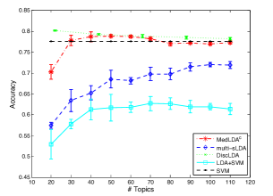
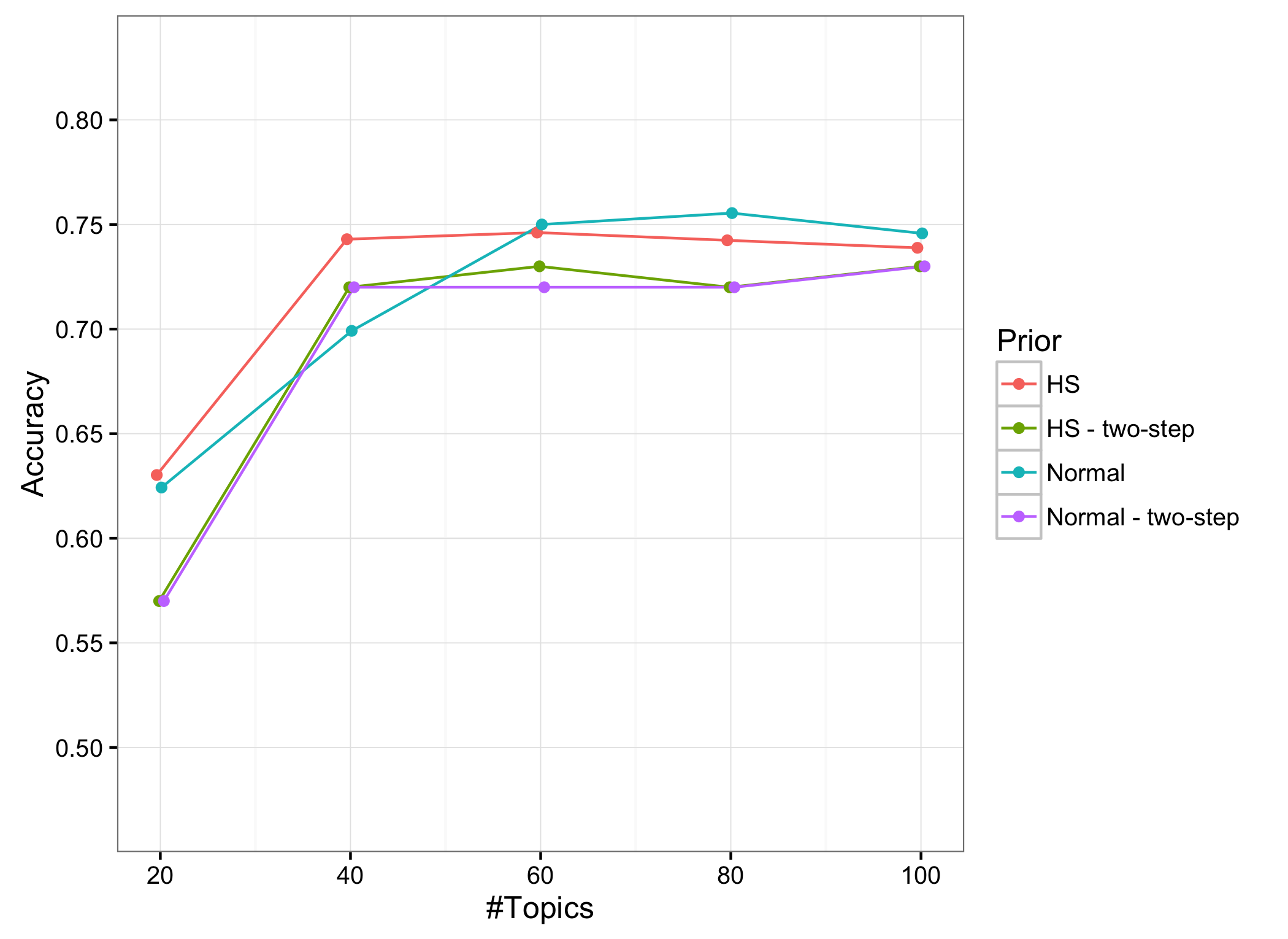
Figure 4.1. Accuracy of MedLDA, taken from Zhu et al. 2012 (left) and accuracy of DOLDA for the 20 Newsgroup test set (right).

The advantage of DOLDA is that it produces interpretable predictions with semantically relevant topics. It is therefore reassuring that DOLDA can compete in accuracy with other less interpretable models, even when the model is dramatically simplified by aggressive Horseshoe shrinkage for interpretational purposes. Our next data set illustrates the interpretational strength of DOLDA. See also our companion paper (Jonsson et al., 2016) in the software engineering literature for further demonstrations of DOLDAs ability to produce interpretable predictions in industrial applications without sacrificing prediction accuracy.

IMDb

Figure 4.2 displays the accuracy on the IMDb dataset as a function of the number of topics. The estimated DOLDA model also contains several other discrete covariates, such as the film’s director and producer. The accuracy of the more aggressive Horseshoe prior is better than the normal prior for all topic sizes. A supervised approach with topics and supervision inferred jointly is again outperforming a two-step approach.

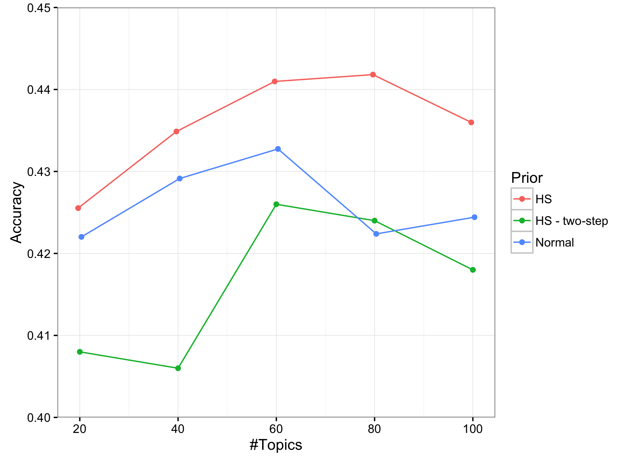
Figure 4.2. Accuracy for DOLDA on the IMDb data with normal and Horseshoe prior and using a two step approach with the Horseshoe prior.

The Horseshoe prior gives somewhat higher accuracy than the normal prior, and incorporating the Horseshoe prior let us handle many additional covariates since the shrinkage prior will act as a type of variable selection.

To illustrate the interpretation of DOLDA we fit a new model using only topics as covariates. Note first in Figure 4.3 how the Horseshoe prior is able to distinguish between so called signal topics and noise topics; the Horseshoe prior is aggressively shrinking a large fraction of the regression coefficient toward zero. This is achieved without the need of setting any hyper-parameters.

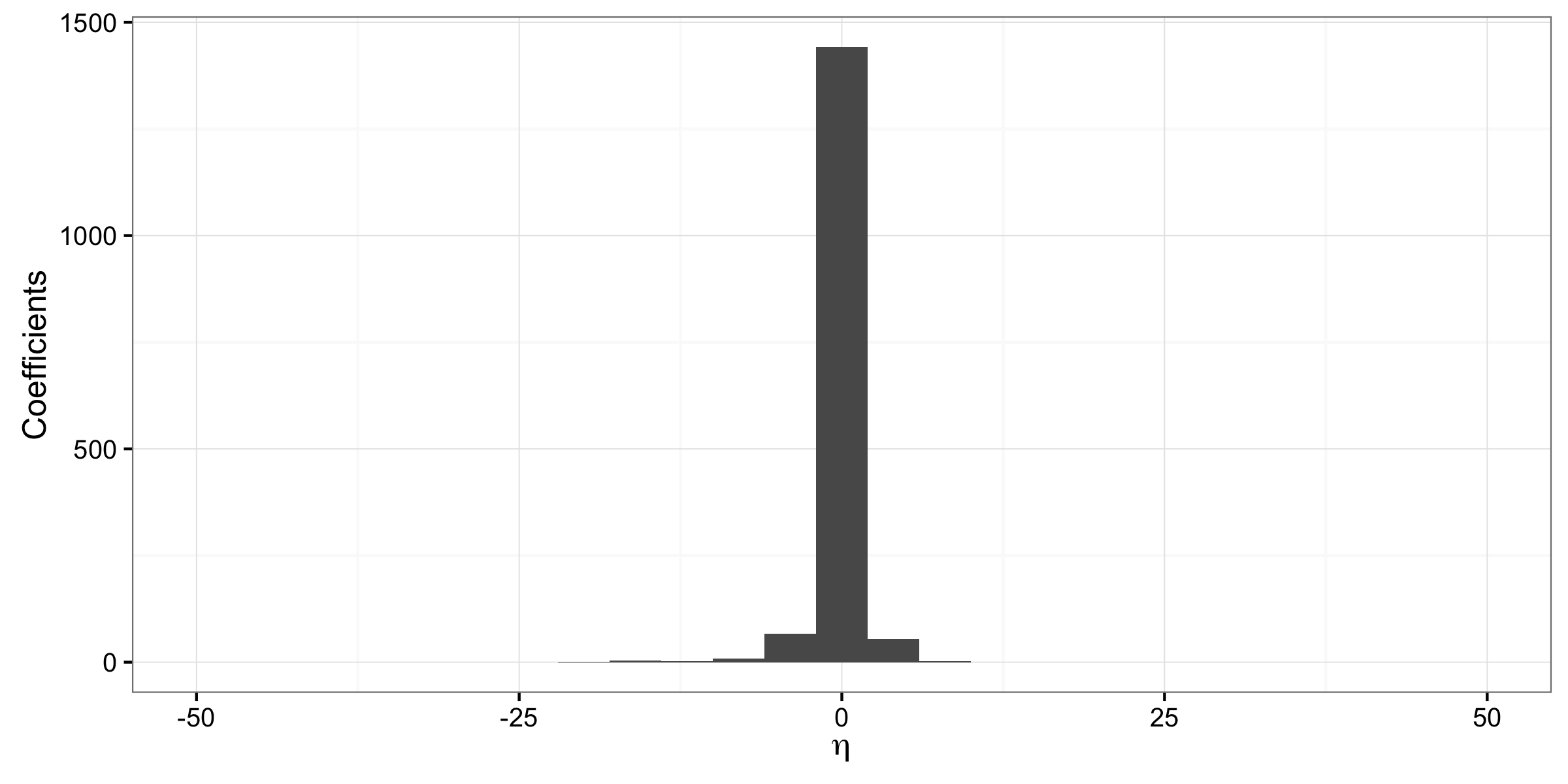
Figure 4.3. Coefficients for the IMDb dataset with 80 topics using the normal prior (left) and the Horseshoe prior (right).

The Horseshoe shrinkage makes it easy to identify the topics that affect a given class. This is illustrated for the Romance genre in the IMDb dataset in Figure 4.4. This genre consists of relatively few observations (only 39 movies), and the Horseshoe prior therefore shrinks most coefficients to zero, keeping only one large signal topic that happens to have a negative effect on the Romance genre. The normal prior on the other hand gives a much more dense, and therefore much less interpretable solution.

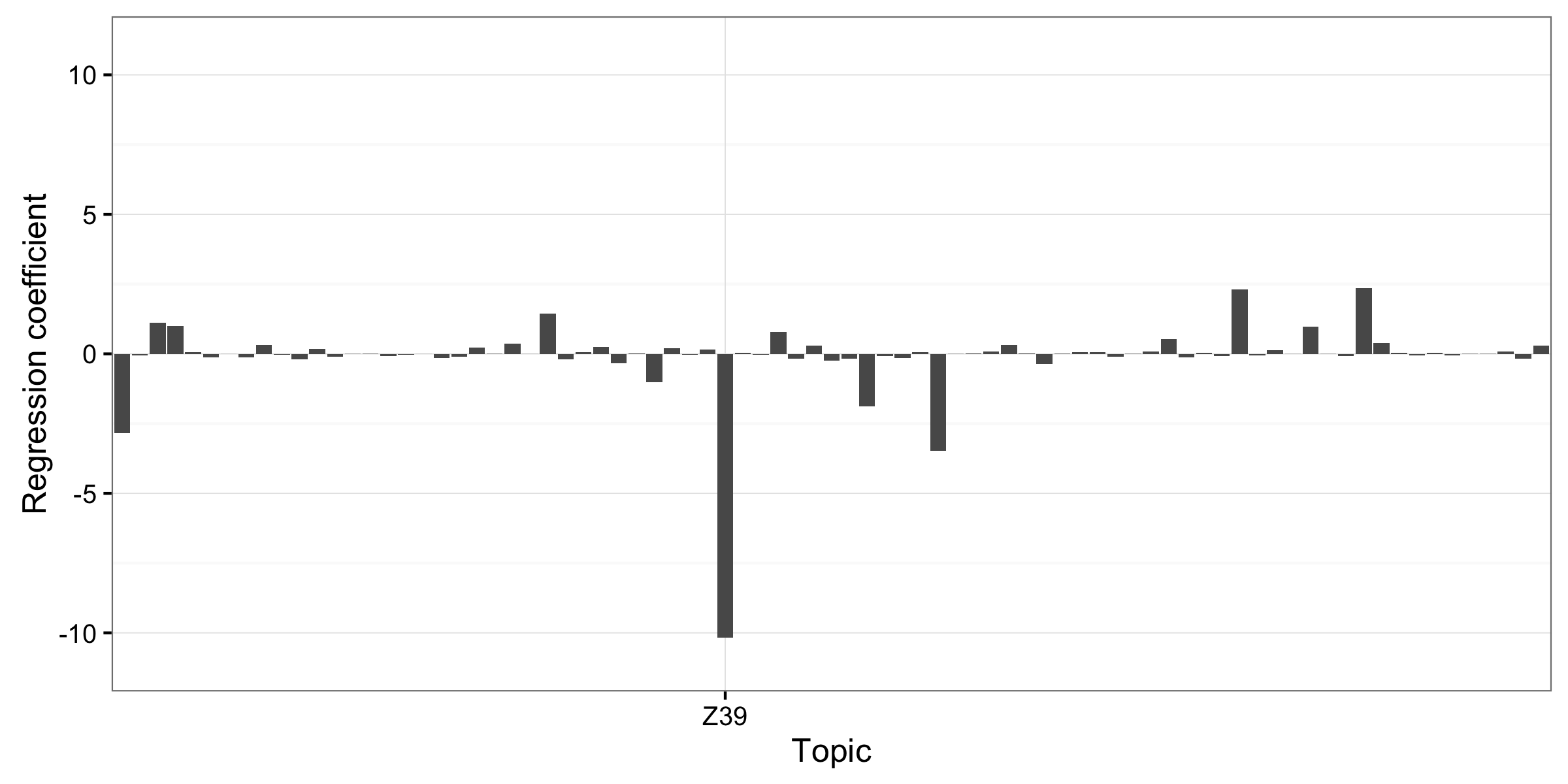
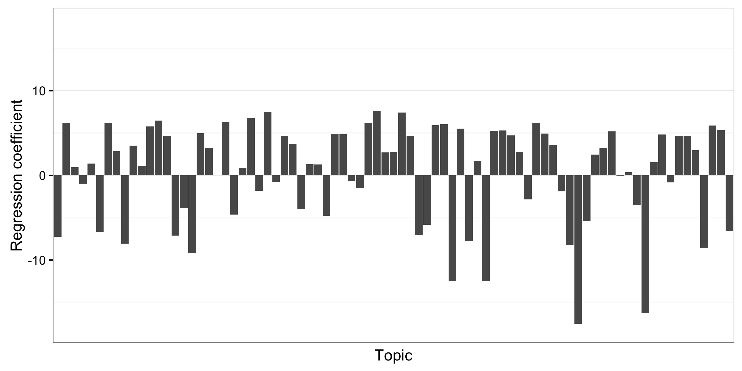
Figure 4.4. Coefficients for the genre Romance in the IMDb dataset with 80 topics using the Horseshoe prior (upper) and a normal prior (below).

Digging deeper in the interpretation of what triggers a Romance genre prediction, Table 3 shows the 10 top word for Topic 39. From this table it is clear that the signal topic identified using the Horseshoe prior is some sort of “crime” topic that is negatively correlated with the Romance genre, something that makes intuitive sense. The crime topic is clearly expected to be positively related to the Crime genre, and Figure 4.5 shows that this is indeed the case.

Topic 33	earth space planet alien human future years world time mission
Topic 39	police murder detective killer case investigation crime crimes solve murdered

Table 3. Top words in topics using the Horseshoe prior.

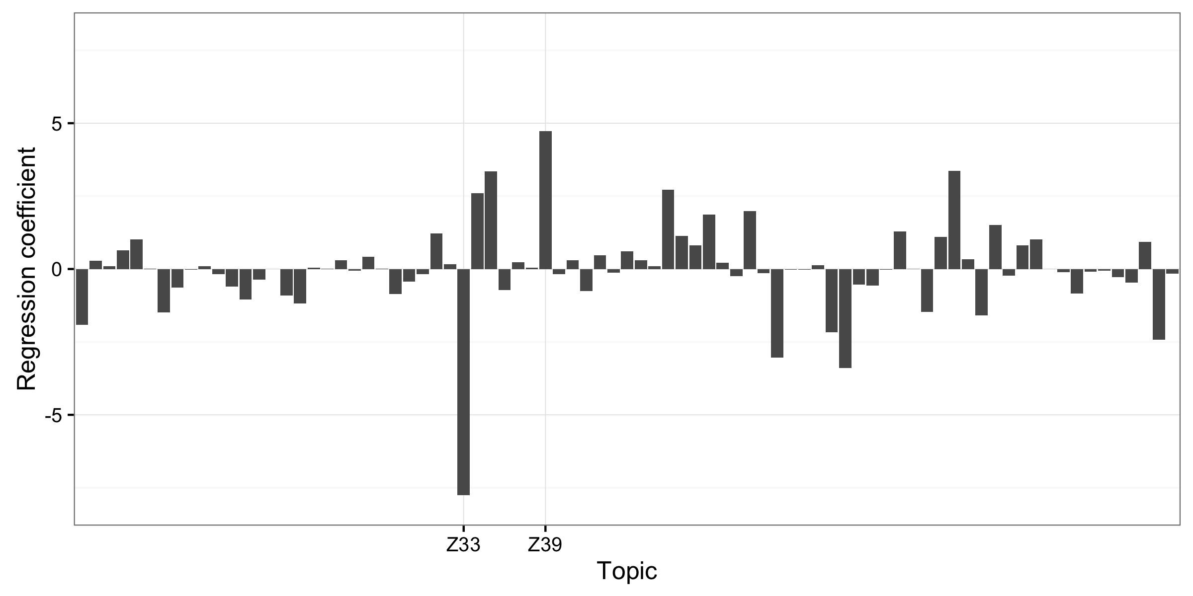
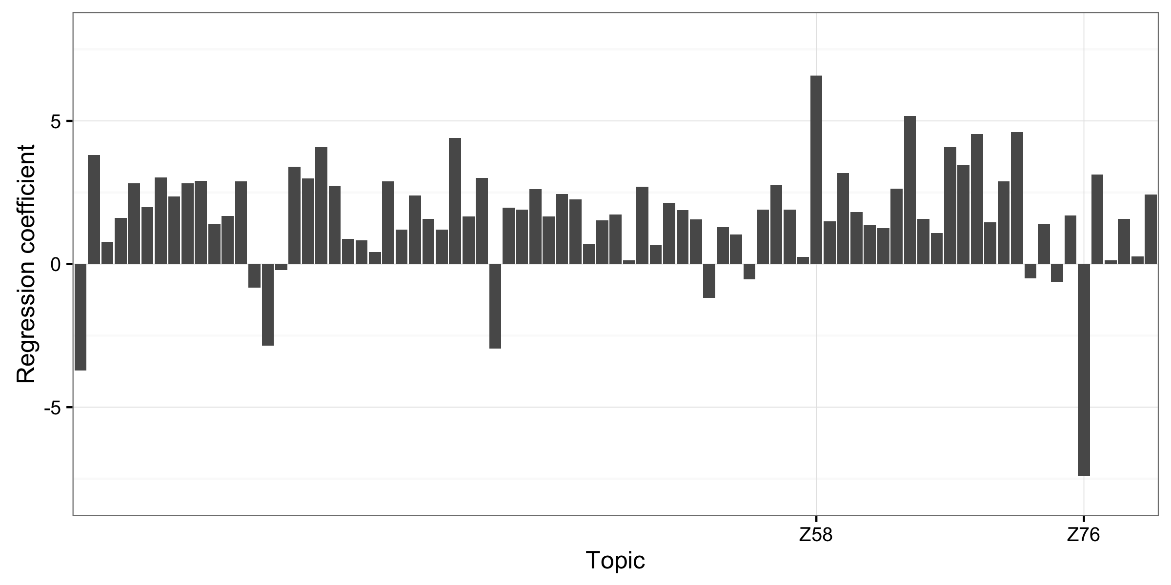
Figure 4.5. Regression coefficients for the class Crime for the IMDb dataset with 80 topics using the Horseshoe prior (upper) and a normal prior (below).

We can also from Figure 4.5 see that Topic 33 is negatively correlated with the Crime genre. In Table 3 we can see that Topic 33 seems to be some sort of Sci-Fi topic containing top words such as “space”, “alien” and “future”. This topic has the largest positive correlation with the Sci-Fi movie genre, which again makes intuitive sense.

5. Conclusions

Several supervised topic models have recently been proposed with the purpose to identify topics that can successfully be used to classify documents. We have here proposed DOLDA, a supervised topic model with special emphasis on generating semantically interpretable predictions. An important component of the model to ease interpretation is the DO-probit model without a reference class. By coupling the DO-probit model with an aggressive Horseshoe prior with shrinkage that is allowed to vary over the different classes it is possible to create a highly interpretable classification model. At the same time the DOLDA model comes with very few hyper parameters that needs tuning, something that is needed in many other supervised topic models such as (Jiang et al., 2012; Zhu et al., 2012; Li et al., 2015). Our experiments show that the gain in interpretation from using DOLDA comes with only a small reduction in prediction accuracy compared to the state-of-the art supervised topic models; moreover, DOLDA outperforms other fully Bayesian models such as the original supervised LDA model. It is also clearly shown that learning the topics jointly with the classification part of the model gives more accurate predictions than a two step approach where a topic model is first estimated and a classifier is then trained on the learned topics.

References

- Albert and Chib (1993) Albert, J. H., Chib, S., 1993. Bayesian analysis of binary and polychotomous response data. Journal of the American statistical Association 88 (422), 669–679.
- Blei et al. (2003) Blei, D. M., Ng, A. Y., Jordan, M. I., 2003. Latent dirichlet allocation. the Journal of machine Learning research 3, 993–1022.
- Carvalho et al. (2010) Carvalho, C., Polson, N., Scott, J., 2010. The horseshoe estimator for sparse signals. Biometrika 97, 465–480.
- Castillo et al. (2015) Castillo, I., Schmidt-Hieber, J., Van der Vaart, A., et al., 2015. Bayesian linear regression with sparse priors. The Annals of Statistics 43 (5), 1986–2018.
- Imai and van Dyk (2005) Imai, K., van Dyk, D. A., 2005. A bayesian analysis of the multinomial probit model using marginal data augmentation. Journal of econometrics 124 (2), 311–334.
- Jameel et al. (2015) Jameel, S., Lam, W., Bing, L., 2015. Supervised topic models with word order structure for document classification and retrieval learning. Information Retrieval Journal, 1–48.
- Jiang et al. (2012) Jiang, Q., Zhu, J., Sun, M., Xing, E. P., 2012. Monte carlo methods for maximum margin supervised topic models. In: Advances in Neural Information Processing Systems. pp. 1592–1600.
- Johndrow et al. (2013) Johndrow, J., Dunson, D., Lum, K., 2013. Diagonal orthant multinomial probit models. In: Proceedings of the Sixteenth International Conference on Artificial Intelligence and Statistics. pp. 29–38.
- Jonsson et al. (2016) Jonsson, L., Broman, D., Magnusson, M., Sandahl, K., Villani, M., Eldh, S., 2016. Automatic localization of bugs to faulty components in large scale software systems using bayesian classification. In: IEEE International Conference on Software Quality, Reliability and Security. QRS.
- Li et al. (2015) Li, X., Ouyang, J., Zhou, X., Lu, Y., Liu, Y., 2015. Supervised labeled latent dirichlet allocation for document categorization. Applied Intelligence 42 (3), 581–593.
- Magnusson et al. (2015) Magnusson, M., Jonsson, L., Villani, M., Broman, D., 2015. Parallelizing LDA using Partially Collapsed Gibbs Sampling. arXiv e-prints arXiv:1506.03784.
- Mcauliffe and Blei (2008) Mcauliffe, J. D., Blei, D. M., 2008. Supervised topic models. In: Advances in neural information processing systems. pp. 121–128.
- Parnin and Orso (2011) Parnin, C., Orso, A., 2011. Are automated debugging techniques actually helping programmers? In: Proceedings of the 2011 International Symposium on Software Testing and Analysis. ACM, pp. 199–209.
- Perotte et al. (2011) Perotte, A. J., Wood, F., Elhadad, N., Bartlett, N., 2011. Hierarchically supervised latent dirichlet allocation. In: Advances in Neural Information Processing Systems. pp. 2609–2617.
- Polson et al. (2013) Polson, N. G., Scott, J. G., Windle, J., 2013. Bayesian inference for logistic models using pólya–gamma latent variables. Journal of the American Statistical Association 108 (504), 1339–1349.
- Ramage et al. (2009) Ramage, D., Hall, D., Nallapati, R., Manning, C. D., 2009. Labeled LDA: A supervised topic model for credit attribution in multi-labeled corpora. In: Proceedings of the 2009 Conference on Empirical Methods in Natural Language Processing. Vol. 1. Association for Computational Linguistics, pp. 248–256.
- Rubin et al. (2012) Rubin, T. N., Chambers, A., Smyth, P., Steyvers, M., 2012. Statistical topic models for multi-label document classification. Machine learning 88 (1-2), 157–208.
- Zheng et al. (2015) Zheng, X., Yu, Y., Xing, E. P., 2015. Linear time samplers for supervised topic models using compositional proposals. In: Proceedings of the 21th ACM SIGKDD International Conference on Knowledge Discovery and Data Mining. KDD ’15. ACM, New York, NY, USA, pp. 1523–1532.
- Zhu et al. (2012) Zhu, J., Ahmed, A., Xing, E. P., 2012. Medlda: maximum margin supervised topic models. the Journal of machine Learning research 13 (1), 2237–2278.
- Zhu et al. (2013) Zhu, J., Zheng, X., Zhang, B., 2013. Improved bayesian logistic supervised topic models with data augmentation. arXiv preprint arXiv:1310.2408.