A single-electron approach for many-electron dynamics in high-order harmonic generation

Abstract

We present a novel ab-initio single-electron approach to correlated electron dynamics in strong laser fields. By writing the electronic wavefunction as a product of a marginal one-electron wavefunction and a conditional wavefunction, we show that the exact harmonic spectrum can be obtained from a single-electron Schrödinger equation. To obtain the one-electron potential in practice, we propose an adiabatic approximation, i.e. a potential is generated that depends only on the position of one electron. This potential, together with the laser interaction, is then used to obtain the dynamics of the system. For a model Helium atom in a laser field, we show that by using our approach, the high-order harmonic generation spectrum can be obtained to a good approximation.

One of the most interesting phenomena occurring in the interaction of molecules with strong laser fields is the process of high-order harmonic generation (HHG) McPherson et al. (1987); Ferray et al. (1988): a molecule exposed to an infrared driving laser radiates light with a frequency being an integer multiple of the driving frequency, with significant intensities. As the electron dynamics responsible for the light emission is fast, the resulting spectra can be used as an attosecond probe of the dynamics of the molecule.Itatani et al. (2004); Krausz and Ivanov (2009); Smirnova et al. (2009); Haessler et al. (2010, 2011); Salières et al. (2012)

The process of HHG is most easily understood in the 3-step model Schafer et al. (1993); Corkum (1993); Lewenstein et al. (1994), which is a semi-classical single-electron picture: During the laser cycle, an electron first tunnels out of the bound-state region of the molecule. The laser field then accelerates it away and, when the field switches sign, back to the molecule. Finally, the collision of the electron with the molecule leads to the measured emission of high-order harmonics. In practice, a single-active electron approximation Kulander (1987) is often used to calculate spectra: For a suitable model potential, a one-electron Schrödinger equation is solved and the spectrum is calculated. Finding an appropriate potential is a challenge Abu-samha and Madsen (2010); Awasthi and Saenz (2010) and the correct incorporation of many-electron effects poses an obstacle.

Clearly, the merit of the single-active electron approximation is that it is only necessary to solve a single-particle Schrödinger equation. In this article, we want to retain this crucial advantage, but ask the question: Is it possible to obtain the relevant dynamical data to calculate the HHG spectra from a single-electron calculation not only approximately, but exactly? The answer is yes, and the way how we answer this question suggests a strategy to obtain the corresponding potential in practice.

Our approach is inspired by the exact factorization (EF) of a time-dependent molecular wavefunction into a marginal nuclear and a conditional electronic wavefunction Cederbaum (2008); Abedi et al. (2010, 2012, 2013); Agostini et al. (2013); Abedi et al. (2014); Agostini et al. (2014, 2015a); Min et al. (2015); Scherrer et al. (2015); Suzuki et al. (2015); Agostini et al. (2015b); Khosravi et al. (2015), see also the time-independent case Hunter (1975, 1981); Gidopoulos and Gross (2014); Chiang et al. (2014); Min et al. (2014); Requist and Gross (2015). The EF is normally used to separate the molecular wavefunction into a nuclear and an electronic wavefunction. However, the EF was also used to describe electron localization in H${}_{2}^{+}$ by strong lasers Suzuki et al. (2014) (by formally reversing the role of nuclei and electrons), to introduce time into the stationary Schrödinger equation Arce (2012), and to factor identical particles.Hunter (1986); A. Buijse et al. (1989)

We build upon that latter approach and apply the EF to the time-dependent electronic wavefunction to obtain an exact single-electron equation. Complementary to this, we use an expansion in adiabatic states (ASE), the analogue of the Born-Huang expansion Born and Huang (1954), as a tool for analysis. Ultimately, we apply an adiabatic approximation reminiscent of the Born-Oppenheimer approximation Born and Oppenheimer (1927) and check its validity.

For this purpose, we consider a system of 2 electrons at positions $r_{1},r_{2}$ in the external field of the laser and of the (clamped) nuclei, and, for simplicity, spin is not considered explicitly. The interaction of the electrons with the laser is treated in the dipole approximation, so that the system is described by the Schrödinger equation

$$i\partial_{t}\psi=\left(-\frac{\partial_{1}^{2}}{2}-\frac{\partial_{2}^{2}}{2}+V(r_{1},r_{2})+(r_{1}+r_{2})F(t)\right)\psi$$ (1)

for $\psi(r_{1},r_{2},t)$. Here, $\partial_{i}$ is the gradient w.r.t. $r_{i}$ and $V(r_{1},r_{2})$ includes the electron-electron repulsion and the interaction of the electrons with the clamped nuclei. Atomic units are used throughout the article.

The restriction to 2 electrons is done only for convenience of notation, but the method described below can be applied to any number of electrons. Typically, $r_{1}$ are the coordinates of one electron and $r_{2}$ are those of the other electrons, but $r_{1}$ may also contain coordinates of more than one electron. This is important if two- or many-electron observables are of interest, like double ionization, etc.

In the EF, it is used that any joint probability distribution function (PDF) depending on several variables can be written as a product of a marginal PDF and a conditional PDF. The marginal PDF depends on a subset of the variables, and the conditional PDF depends on the other ones and conditionally on the subset. Thus, the time-dependent wavefunction is written as a product

$$\psi(r_{1},r_{2},t) =\chi(r_{1},t)\phi(r_{2},t|r_{1})$$ (2)

with a marginal wavefunction

$$\chi(r_{1},t) =e^{-iS(r_{1},t)}\sqrt{\rho(r_{1},t)}$$ (3)

and a conditional wavefunction

$$\phi_{j}(r_{2},t|r_{1}) =\psi(r_{1},r_{2},t)/\chi(r_{1},t).$$ (4)

The one-electron density $\rho(r_{1},t)=\left<\psi\vphantom{\psi}\right|\left.\psi\vphantom{\psi}\right>_{2}$ is the marginal PDF which gives the probability of finding an electron at $r_{1}$ independent of the other electron. Here, $\left<\cdot\vphantom{\cdot}\right|\left.\cdot\vphantom{\cdot}\right>_{i}$ indicates integration over $r_{i}$, For $\phi_{j}$ the partial normalization condition $\left<\phi_{j}\vphantom{\phi_{j}}\right|\left.\phi_{j}\vphantom{\phi_{j}}\right>_{2}=1$ is fulfilled for all $r_{1},t$. Thus, $|\phi_{j}(r_{2},t|r_{1})|^{2}$ is a conditional PDF, i.e., given an electron at $r_{1}$, it gives the probability of finding the other electron at $r_{2}$.

The equation of motion for the marginal wavefunction is Abedi et al. (2012)

$$i\partial_{t}\chi =\left(-\frac{(\partial_{1}+A(r_{1},t))^{2}}{2}+\epsilon(r_{1},t)\right)\chi$$ (5)

with the vector potential

$$A(r_{1},t)=\operatorname{Im}\left<\phi\vphantom{\partial_{1}\phi}\right|\left.\partial_{1}\phi\vphantom{\phi}\right>_{2}$$ (6)

and scalar potential

$$\epsilon(r_{1},t)=\left<\phi\vphantom{-\frac{\partial_{2}^{2}}{2}+V(r_{1},r_{2})\phi}\right|-\frac{\partial_{2}^{2}}{2}+V(r_{1},r_{2})\left|\phi\vphantom{\phi-\frac{\partial_{2}^{2}}{2}+V(r_{1},r_{2})}\right>_{2}+\operatorname{Im}\left<\phi\vphantom{\partial_{t}\phi}\right|\left.\partial_{t}\phi\vphantom{\phi}\right>_{2}\\ +\frac{\left<\partial_{1}\phi\vphantom{\partial_{1}\phi}\right|\left.\partial_{1}\phi\vphantom{\partial_{1}\phi}\right>_{2}-A(r_{1},t)^{2}}{2}+\left(r_{1}+\left<\phi\vphantom{r_{2}\phi}\right|r_{2}\left|\phi\vphantom{\phi r_{2}}\right>_{2}\right)F(t).$$ (7)

The latter consists of a part similar to a Born-Oppenheimer potential (albeit with the exact, time-dependent conditional wavefunction $\phi$), a gauge-dependent part, a part that is related to a Fubini-Study metricBerry (1989), and the laser interaction. The gauge transformation

$$\tilde{\chi}=e^{-\tilde{S}(r_{1},t)}\chi,~{}~{}~{}\tilde{\phi}=e^{\tilde{S}(r_{1},t)}\phi$$ (8)

leaves the total wavefunction and the equations of motion unchanged but transforms the vector and scalar potential as $\tilde{A}=A+\partial_{1}\tilde{S}$ and $\tilde{\epsilon}=\epsilon+\partial_{t}\tilde{S}$, respectively. The equation of motion for $\phi$ is not being used in the present context and can be found, for example, in Abedi et al. (2012).

The EF formulation is the exact single-electron picture that we are looking for. As was shown in Abedi et al. (2010), $\chi$ and $\phi$ are unique up to the gauge transformation (8), and $\chi$ gives the correct one-electron density and one-electron current density and, hence, yields the exact HHG spectrum. The EF may thus be seen as the, so far missing, formal justification of the single-active electron approach. Rohringer et al. (2006)

In the ASE, the wavefunction is written as

$$\psi(r_{1},r_{2},t) =\sum_{j=0}^{\infty}\chi_{j}^{\rm ASE}(r_{1},t)\phi_{j}^{\rm ASE}(r_{2}|r_{1}),$$ (9)

where the wavefunctions $\phi_{j}^{\rm ASE}(r_{2}|r_{1})$ are obtained as stationary states for fixed $r_{1}$,

$$\epsilon_{j}^{\rm ASE}(r_{1})\phi_{j}^{\rm ASE} =\left(-\frac{\partial_{2}^{2}}{2}+V(r_{1},r_{2})\right)\phi_{j}^{\rm ASE}.$$ (10)

Clearly, the wavefunctions $\phi_{j}^{\rm ASE}$ are analogous to the Born-Oppenheimer states in the electron-nuclear case. Ansatz (9) leads to coupled equations of motion for the coefficients $\chi_{j}^{\rm ASE}$ Malhado et al. (2014). The analogue of the Born-Oppenheimer approximation for a selected state $k$ is neglect of the coupling terms, i.e.

$$i\partial_{t}\chi^{\rm AE} =\left(-\frac{\partial_{1}^{2}}{2}+\epsilon_{k}^{\rm ASE}(r_{1})+V_{L}(r_{1},t)\right)\chi^{\rm AE},$$ (11)

with the laser interaction

$$V_{L}(r_{1},t) =\left(r_{1}+\left<\phi_{k}^{\rm ASE}\vphantom{r_{2}\phi_{k}^{\rm ASE}}\right|\left.r_{2}\phi_{k}^{\rm ASE}\vphantom{\phi_{k}^{\rm ASE}}\right>\right)F(t).$$ (12)

Equation (11) is our proposal for a single-electron approach to the electron dynamics in strong laser fields. For $N$ electrons, we propose to find the stationary state for one electron fixed at position $r_{1}$ by solving (10) for a suitable state $k$. Then, with the potential generated by varying $r_{1}$, the dynamics of the full $N$-electron system is replaced by the dynamics of the marginal single-electron system obtained from (11). We call the dynamics arising from (11) the adiabatic electron (AE) approximation. The AE approximation takes into account the dynamics of the cation as well as the effect of the cation on the ionized electron. In contrast to the single-active electron approximation, it gives a unique procedure for obtaining the single-electron potential for any molecular system.

As all electrons have the same mass, the AE approximation (11) is not as generically useful as the Born-Oppenheimer approximation. Also, it breaks the anti-symmetry of the electronic wavefunction, albeit only w.r.t. the one electron at $r_{1}$. For the electrons in the set $r_{2}$, the symmetry requirements are obeyed. In situations like ionization and HHG, when one electron moves far away from the rest, the lack of anti-symmetrization of one electron with the wavefunction of the remaining cation is not expected to be a serious restriction for the description of the process.

To test the AE approximation, we study a numerically exactly solvable model of two electrons in an atom. We choose the model of Shi-Lin and Ting-Yun (2013): A helium atom is modeled by the soft-Coulomb interaction potentials

$$V(r_{1},r_{2}) =\frac{1}{\sqrt{(r_{1}-r_{2})^{2}+c}}-\sum_{j=1}^{2}\frac{2}{\sqrt{r_{j}^{2}+c}}$$ (13)

where $r_{1},r_{2}$ are now the coordinates of electron 1 and 2, each in one dimension. The laser pulse is a 12-cycle pulse $F(t)=F_{0}\cos(\omega t)f(t)$, where $\tau=2\pi/\omega$ is the laser period and $f(t)$ increases (decreases) linearly from 0 to 1 during the first (last) two cycles. The laser frequency $\omega$ corresponds to a wavelength of 530 nm, and the laser amplitude $F_{0}$ yields a maximum intensity of $6.88\times 10^{14}$ $W/cm^{2}$. The interaction parameter is $c=0.55$ $a_{0}^{2}$. For the calculations we used at least the spacial and temporal grid of Shi-Lin and Ting-Yun (2013), with the same mask region (the wavefunction is absorbed if $|r_{i}|>$ 70 $a_{0}$). The static eigenvalue problems were solved by implicitly restarted Arnoldi methods Lehoucq et al. (1998) as implemented in SciPy Jones et al. (01), while the time propagation was performed with a split-operator method Feit et al. (1982).

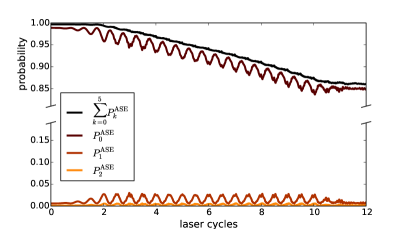
Figure 1: Occupation numbers $P_{j}^{\rm ASE}$ (14) of the adiabatic state expansion (9) and partial sum for the lowest 6 states (visually indistinguishable from the norm of the wavefunction).

First, we compute the occupation numbers

$$P_{j}^{\rm ASE}(t)=\left<\chi_{j}^{\rm ASE}\vphantom{\chi_{j}^{\rm ASE}}\right|\left.\chi_{j}^{\rm ASE}\vphantom{\chi_{j}^{\rm ASE}}\right>_{1}$$ (14)

of the ASE states from the exact wavefunction, shown in figure 1. In contrast to an expansion of the full wavefunction in terms of the eigenstates of the system, there are no “symmetry selection rules” in the ASE and all states can be occupied. The wavefunction is mainly composed of the ASE ground state, with only small contributions from the first and second excited state and a periodic population transfer between ground and excited states with a period of half the laser period. Consequently, an AE approximation to consider only the ground state for the dynamics should be applicable.

The occupation numbers give only an incomplete picture: They do not reveal that only certain parts of the full wavefunction are represented well by a truncated expansion. In figure 2 we show a logarithmic plot of the density after half of the laser pulse is over (at a time where the field is maximal). In the top row of the figure, the exact density and the density obtained from an ASE truncated after 3 states are shown. Clearly, the symmetry properties of the wavefunction are lost and any two-electron observables, notably double ionization (the region where both $|r_{1}|$ and $|r_{2}|$ are large), cannot be described by the truncated wavefunction. In such a case, a repeated factorization of the many-electron wavefunction, like described in Cederbaum (2015), may be useful to derive computational methods.

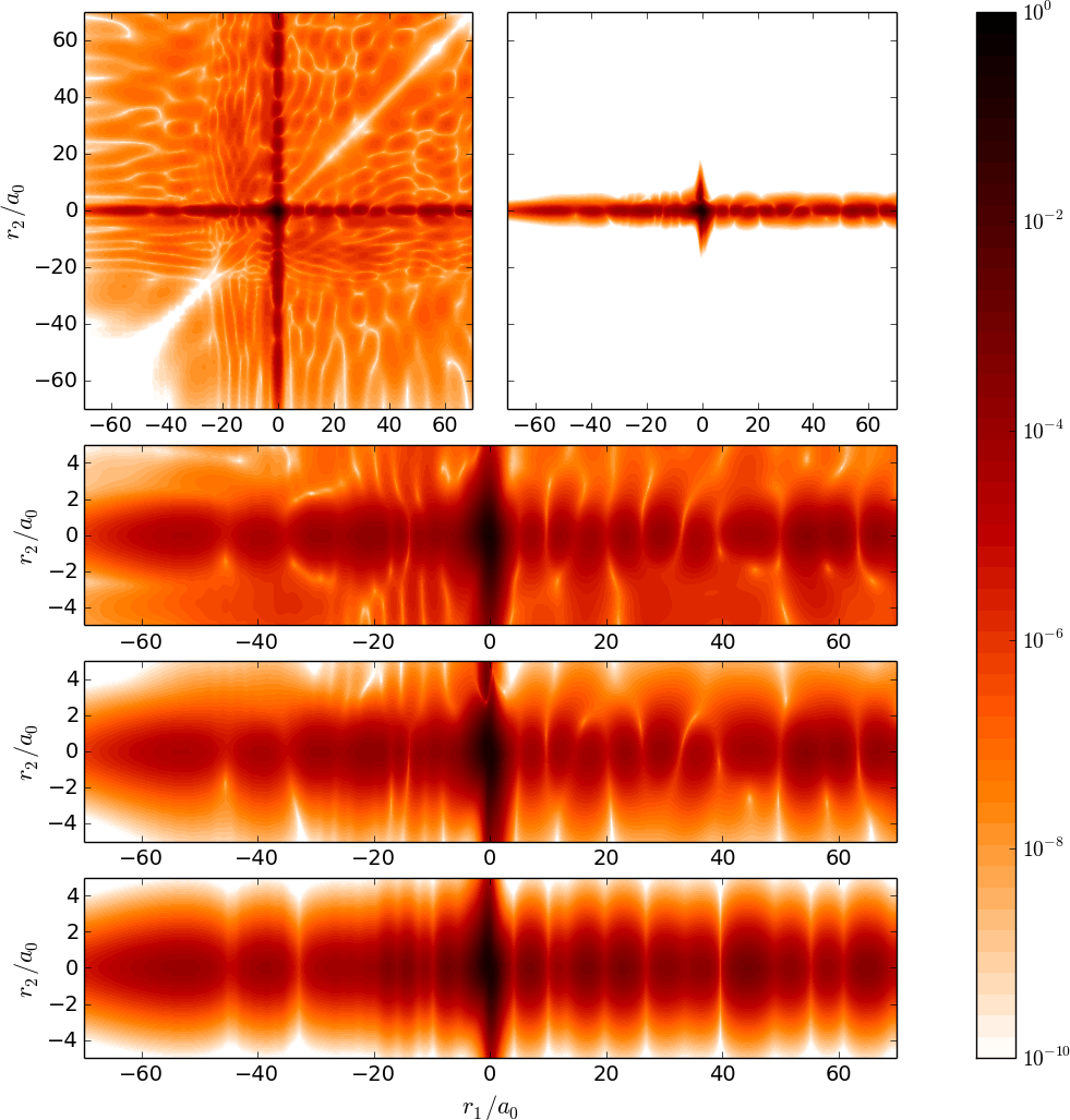
Figure 2: Top: Logarithmic plot of the exact density $|\psi(r_{1},r_{2},t)|^{2}$ for $t=6\tau$ (after half of the pulse) and of the density $|\psi^{(3)}(r_{1},r_{2},t)|^{2}$ for the expansion of $\psi$ in the ASE, (9), including only the lowest 3 states, $\psi^{(3)}=\sum_{k=0}^{2}\chi_{j}^{\rm ASE}(r_{1},t)\phi_{j}^{\rm ASE}(r_{2}|r_{1})$. Below: Blow up of $|\psi|^{2}$, $|\psi^{(3)}|^{2}$, and the density of the adiabatic electron approximation $|\psi^{\rm AE}(r_{1},r_{2},t)|^{2}$ for $\psi^{\rm AE}=\chi^{\rm AE}(r_{1},t)\phi_{0}^{\rm ASE}(r_{2}|r_{1})$.

The loss of the symmetry properties is by construction: We allow $r_{1}$ to become as large as necessary, but along $r_{2}$ we compute the bound states. The energetically lowest bound states are localized in the region of small $r_{2}$. Hence, for describing large excursions along $r_{2}$ (which is necessary when we want to recover the correct symmetry of the wavefunction) we need highly excited states and continuum states.

However, for small $r_{2}$ the density is well-reproduced by the truncated expansion. The two central panels of figure 2 show a blow-up of the respective region. Details of the exact density are already well reproduced by the first few states of the expansion and inclusion of a few further states would make the dynamics in this region almost indistinguishable from the exact one. Hence, we conclude that observables related to a large excursion of only one electron can be described with a truncated expansion, as intuitively expected.

In the bottom panel of figure 2, a plot of the density at $t=6\tau$ is shown for a propagation in the AE approximation, i.e., obtained from solving (11) using the ground state $\phi_{0}$ of (10). The density is symmetric w.r.t. $r_{2}$ because $\phi_{0}$ has this property. While there are discrepancies from the exact density, the qualitative structure is reproduced, even on this logarithmic scale.

The spectrum obtained from the AE approximation is calculated as the Fourier transform of the dipole acceleration Bandrauk et al. (2009),

$$\Gamma(\omega)=\frac{2}{T^{2}\omega^{4}}\left|\int\limits_{0}^{T}\partial_{t}^{2}\left<r_{1}\rho\right>_{1}e^{-i\omega t}dt\right|,$$ (15)

and shown in figure 3. We choose (15) to compute the spectrum because it only needs the directly accessible one-electron density $\rho(r_{1},t)$, but in principle other methods can be used. The factor 2 is the number of electrons in the system.

As can be seen from the figure, the overall features of the exact spectrum are well reproduced, especially the frequency region from harmonic 9 to harmonic 43. Only initially and close to the cutoff frequency the approximate spectrum deviates from the exact one. The discrepancies can be explained by a comparison between the exact potential $\epsilon$ of (7) and the approximate potential $\epsilon_{0}^{\rm ASE}+V_{L}$ of (11), for a gauge where the exact vector potential $A=0$. While they are almost indistinguishable in the bound-state region, for the region of the barrier that the electron has to tunnel through we find $\epsilon\geq\epsilon_{0}^{\rm ASE}+V_{L}$. The difference is small but noticeable in the dynamics, because it leads to higher values of the density outside the core region. In other words, during the time of maximum field amplitude the electron has a higher chance to tunnel out of the bound-state region than it should have. Furthermore, there are spikesCzub and Wolniewicz (1978); Hunter (1981); Chiang et al. (2014) and stepsElliott et al. (2012); Abedi et al. (2013) in the potential. They are signs of non-adiabatic effects, i.e. they show that restriction of the dynamics to only the ground state potential leads to errors in the dynamics.

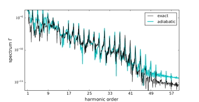
Figure 3: Logarithmic plots of the spectrum (15) for the exact dynamics and the dynamics obtained from the adiabatic electron approximation (11), for the model of Shi-Lin and Ting-Yun (2013).

Finally, we also made a calculation for one of the best exact 2-electron models available in the literature: The N₂ model of Sukiasyan et al. (2009, 2010) for a system of two fixed nuclei and two electrons that may move each in two dimensions, in an intense 10-cycle laser pulse. Figure 4 shows how the spectrum of the AE approximation compares to the exact spectrum. The harmonic intensities seem to be well reproduced for most harmonics, at least on the logarithmic scale of the figure.

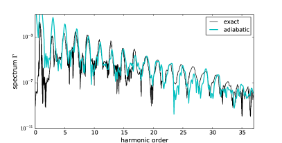
Figure 4: Logarithmic plot of the exact and the adiabatic electron dynamics (11), for the model of Sukiasyan et al. (2009). The exact spectrum was extracted graphically from FIG. 1 (a) of Sukiasyan et al. (2009).

In summary, we have shown that the HHG spectra can in principle be obtained from a single-electron Schrödinger. A promising way to obtain the corresponding potential in practice is to make the adiabatic electron approximation, an extension of the concept of the Born-Oppenheimer approximation to systems of identical particles. The main advantage of this approach is that only a single-electron Schrödinger equation needs to be solved, that all many-electron effects are included to a certain extent, and that it proposes a unique way of obtaining the required potential: The energy of the system with one clamped negative charge needs to be determined for various positions of the clamped charge. This problem is a standard, albeit challenging one in electronic structure theory.

Furthermore, our proposed approach can be systematically improved by the transfer of concepts of non-adiabatic molecular dynamics to systems of identical particles. The large knowledge base in this field makes us confident that an appropriate approximation to the exact electron factorization can be found for many different molecular systems in strong electric laser fields.

References

- McPherson et al. (1987) A. McPherson, G. Gibson, H. Jara, U. Johann, T. S. Luk, I. A. McIntyre, K. Boyer, and C. K. Rhodes, J. Opt. Soc. Am. B 4, 595 (1987).
- Ferray et al. (1988) M. Ferray, A. L’Huillier, X. F. Li, L. A. Lompre, G. Mainfray, and C. Manus, Journal of Physics B: Atomic, Molecular and Optical Physics 21, L31 (1988).
- Itatani et al. (2004) J. Itatani, J. Levesque, D. Zeidler, H. Niikura, H. Pépin, J. C. Kieffer, P. B. Corkum, and D. M. Villeneuve, Nature 432, 867 (2004).
- Krausz and Ivanov (2009) F. Krausz and M. Ivanov, Rev. Mod. Phys. 81, 163 (2009).
- Smirnova et al. (2009) O. Smirnova, Y. Mairesse, S. Patchkovskii, N. Dudovich, D. Villeneuve, P. Corkum, and M. Y. Ivanov, Nature 460, 972 (2009).
- Haessler et al. (2010) S. Haessler, J. Caillat, W. Boutu, C. Giovanetti-Teixeira, T. Ruchon, T. Auguste, Z. Diveki, P. Breger, A. Maquet, B. Carré, R. Taïeb, and P. Salières, Nature Physics 6, 200 (2010).
- Haessler et al. (2011) S. Haessler, P. Salières, and J. Caillat, J. Phys. B: At. Opt. Phys. 44, 203001 (2011).
- Salières et al. (2012) P. Salières, A. Maquet, S. Haessler, J. Caillat, and R. Taïeb, Rep. Prog. Phys. 75, 062401 (2012).
- Schafer et al. (1993) K. J. Schafer, B. Yang, L. F. DiMauro, and K. C. Kulander, Phys. Rev. Lett. 70, 1599 (1993).
- Corkum (1993) P. B. Corkum, Phys. Rev. Lett. 71, 1994 (1993).
- Lewenstein et al. (1994) M. Lewenstein, P. Balcou, M. Y. Ivanov, A. L’Huillier, and P. B. Corkum, Phys. Rev. A 49, 2117 (1994).
- Kulander (1987) K. C. Kulander, Phys. Rev. A 35, 445 (1987).
- Abu-samha and Madsen (2010) M. Abu-samha and L. B. Madsen, Phys. Rev. A 81, 033416 (2010).
- Awasthi and Saenz (2010) M. Awasthi and A. Saenz, Phys. Rev. A 81, 063406 (2010).
- Cederbaum (2008) L. S. Cederbaum, J. Chem. Phys 128, 124101 (2008).
- Abedi et al. (2010) A. Abedi, N. T. Maitra, and E. K. U. Gross, Phys. Rev. Lett. 105, 123002 (2010).
- Abedi et al. (2012) A. Abedi, N. T. Maitra, and E. K. U. Gross, J. Chem. Phys. 137, 22A530 (2012).
- Abedi et al. (2013) A. Abedi, F. Agostini, Y. Suzuki, and E. K. U. Gross, Phys. Rev. Lett. 110, 263001 (2013).
- Agostini et al. (2013) F. Agostini, A. Abedi, Y. Suzuki, and E. K. U. Gross, Mol. Phys. 111, 3625 (2013).
- Abedi et al. (2014) A. Abedi, F. Agostini, and E. K. U. Gross, Europhys. Lett. 106, 33001 (2014).
- Agostini et al. (2014) F. Agostini, A. Abedi, and E. K. U. Gross, J. Chem. Phys. 141, 214101 (2014).
- Agostini et al. (2015a) F. Agostini, A. Abedi, Y. Suzuki, S. K. Min, N. T. Maitra, and E. K. U. Gross, J. Chem. Phys. 142, 084303 (2015a).
- Min et al. (2015) S. K. Min, F. Agostini, and E. K. U. Gross, Phys. Rev. Lett. 115, 073001 (2015).
- Scherrer et al. (2015) A. Scherrer, F. Agostini, D. Sebastiani, E. K. U. Gross, and R. Vuilleumier, J. Chem. Phys. 143, 074106 (2015).
- Suzuki et al. (2015) Y. Suzuki, A. Abedi, N. T. Maitra, and E. K. U. Gross, Phys. Chem. Chem. Phys. 17, 29271 (2015).
- Agostini et al. (2015b) F. Agostini, S. K. Min, and E. K. U. Gross, Ann. Phys. 527, 546 (2015b).
- Khosravi et al. (2015) E. Khosravi, A. Abedi, and N. T. Maitra, Phys. Rev. Lett. 115, 263002 (2015).
- Hunter (1975) G. Hunter, Int. J. Quant. Chem. 9, 237 (1975).
- Hunter (1981) G. Hunter, Int. J. Quant. Chem. 19, 755 (1981).
- Gidopoulos and Gross (2014) N. I. Gidopoulos and E. K. U. Gross, Phil. Trans. R. Soc. A 372, 20130059 (2014).
- Chiang et al. (2014) Y.-C. Chiang, S. Klaiman, F. Otto, and L. S. Cederbaum, J. Chem. Phys. 140, 054104 (2014).
- Min et al. (2014) S. K. Min, A. Abedi, K. S. Kim, and E. K. U. Gross, Phys. Rev. Lett. 113, 263004 (2014).
- Requist and Gross (2015) R. Requist and E. K. U. Gross, pre-print (2015), arXiv:1506.09193 [physics.chem-ph].
- Suzuki et al. (2014) Y. Suzuki, A. Abedi, N. T. Maitra, K. Yamashita, and E. K. U. Gross, Phys. Rev. A 89, 040501 (2014).
- Arce (2012) J. C. Arce, Phys. Rev. A 85, 042108 (2012).
- Hunter (1986) G. Hunter, Int. J. Quant. Chem. 29, 197 (1986).
- A. Buijse et al. (1989) M. A. Buijse, E. J. Baerends, and J. G. Snijders, Phys. Rev. A 40, 4190 (1989).
- Born and Huang (1954) M. Born and K. Huang, Dynamical Theory of Crystal Lattices (Oxford University Press, 1954).
- Born and Oppenheimer (1927) M. Born and R. Oppenheimer, Ann. Phys. 389, 457 (1927).
- Berry (1989) M. V. Berry, in Geometric Phases in Physics, edited by A. Shapere and F. Wilcek (World Scientific, 1989).
- Rohringer et al. (2006) N. Rohringer, A. Gordon, and R. Santra, Phys. Rev. A 74, 043420 (2006).
- Malhado et al. (2014) J. a. P. Malhado, M. J. Bearpark, and J. T. Hynes, Frontiers in Chemistry 2, 97 (2014).
- Shi-Lin and Ting-Yun (2013) H. Shi-Lin and S. Ting-Yun, Chinese Physics B 22, 013101 (2013).
- Lehoucq et al. (1998) R. B. Lehoucq, D. C. Sorensen, and C. Yang, ARPACK USERS GUIDE: Solution of Large Scale Eigenvalue Problems by Implicitly Restarted Arnoldi Methods (SIAM, Philadelphia, PA, 1998).
- Jones et al. (01 ) E. Jones, T. Oliphant, P. Peterson, et al., “SciPy: Open source scientific tools for Python (www.scipy.org),” (2001–).
- Feit et al. (1982) M. Feit, J. Fleck, and A. Steiger, Journal of Computational Physics 47, 412 (1982).
- Cederbaum (2015) L. S. Cederbaum, Chem. Phys. 457, 129 (2015).
- Bandrauk et al. (2009) A. D. Bandrauk, S. Chelkowski, D. J. Diestler, J. Manz, and K.-J. Yuan, Phys. Rev. A 79, 023403 (2009).
- Czub and Wolniewicz (1978) J. Czub and L. Wolniewicz, Molecular Physics 36, 1301 (1978).
- Elliott et al. (2012) P. Elliott, J. I. Fuks, A. Rubio, and N. T. Maitra, Phys. Rev. Lett. 109, 266404 (2012).
- Sukiasyan et al. (2009) S. Sukiasyan, C. McDonald, C. Destefani, M. Y. Ivanov, and T. Brabec, Phys. Rev. Lett. 102, 223002 (2009).
- Sukiasyan et al. (2010) S. Sukiasyan, S. Patchkovskii, O. Smirnova, T. Brabec, and M. Y. Ivanov, Phys. Rev. A 82, 043414 (2010).