Limit theorems for critical first-passage percolation on the triangular lattice

Abstract

Consider (independent) first-passage percolation on the sites of the triangular lattice $\mathbb{T}$ embedded in $\mathbb{C}$. Denote the passage time of the site $v$ in $\mathbb{T}$ by $t(v)$, and assume that $P(t(v)=0)=P(t(v)=1)=1/2$. Denote by $b_{0,n}$ the passage time from 0 to the halfplane $\{v\in\mathbb{T}:\mbox{Re}(v)\geq n\}$, and by $T(0,nu)$ the passage time from 0 to the nearest site to $nu$, where $|u|=1$. We prove that as $n\rightarrow\infty$, $b_{0,n}/\log n\rightarrow 1/(2\sqrt{3}\pi)$ a.s., $E[b_{0,n}]/\log n\rightarrow 1/(2\sqrt{3}\pi)$ and Var$[b_{0,n}]/\log n\rightarrow 2/(3\sqrt{3}\pi)-1/(2\pi^{2})$; $T(0,nu)/\log n\rightarrow 1/(\sqrt{3}\pi)$ in probability but not a.s., $E[T(0,nu)]/\log n\rightarrow 1/(\sqrt{3}\pi)$ and Var$[T(0,nu)]/\log n\rightarrow 4/(3\sqrt{3}\pi)-1/\pi^{2}$. This answers a question of Kesten and Zhang (1997) and improves our previous work (2014). From this result, we derive an explicit form of the central limit theorem for $b_{0,n}$ and $T(0,nu)$. A key ingredient for the proof is the moment generating function of the conformal radii for conformal loop ensemble CLE₆, given by Schramm, Sheffield and Wilson (2009).

Keywords: critical percolation; first-passage percolation; scaling limit; conformal loop ensemble; law of large numbers; central limit theorem

AMS 2010 Subject Classification: 60K35, 82B43

1 Introduction

First-passage percolation (FPP) was introduced by Hammersley and Welsh in 1965 as a model of fluid flow through a random medium. We refer the reader to the recent surveys [3, 10]. In this paper, we continue our study of critical FPP on the triangular lattice $\mathbb{T}$, initiated in [26]. We focus on this particular lattice because our proof relies on the existence of the scaling limit of critical site percolation on $\mathbb{T}$ (see [5, 20]), and this result has not been proved for other planar percolation processes. For recent progress on general planar critical FPP, see [8].

Let $\mathbb{T}=(\mathbb{V},\mathbb{E})$ denote the triangular lattice, where $\mathbb{V}:=\{x+ye^{\pi i/3}\in\mathbb{C}:x,y\in\mathbb{Z}\}$ is the set of sites, and $\mathbb{E}$ is the set of bonds, connecting adjacent sites. Let $\{t(v):v\in\mathbb{V}\}$ be an i.i.d. family of Bernoulli random variables:

$$P[t(v)=0]=P[t(v)=1]=\frac{1}{2}.$$

We call this model Bernoulli critical FPP on $\mathbb{T}$, and denote by $P$ its probability measure. Note that we can view this model as critical site percolation on $\mathbb{T}$ (see e.g. [16, 24] for background on two-dimensional critical percolation). We usually represent it as a random coloring of the faces of the dual hexagonal lattice $\mathbb{H}$, each face centered at $v\in\mathbb{V}$ being blue ($t(v)=0$) or yellow ($t(v)=1$) with probability $1/2$ independently of the others. Sometimes we view the site $v$ as the hexagon in $\mathbb{H}$ centered at $v$.

A path is a sequence $v_{0},\ldots,v_{n}$ of distinct sites of $\mathbb{T}$ such that $v_{k-1}$ and $v_{k}$ are neighbors for all $k=1,\ldots,n$. For a path $\gamma$, we define its passage time as $T(\gamma):=\sum_{v\in\gamma}t(v).$ The first-passage time between two site sets $A,B$ is defined as

$$T(A,B):=\inf\{T(\gamma):\gamma\mbox{ is a path from a site in $A$ to a site in $B$}\}.$$

For any $u\in\mathbb{C}$ with $|u|=1$, denote by $T(0,nu)$ the first-passage time from 0 to the nearest site in $\mathbb{V}$ to $nu$ (if there are more than one such sites, we choose a unique one by some deterministic method). Denote by $b_{0,n}$ the first-passage time from 0 to the halfplane $\{v\in\mathbb{V}:\operatorname{Re}(v)\geq n\}$.

Our main theorem below answers a question proposed by Kesten and Zhang (see (1.10) and (1.11) in [12]):

Theorem 1.1.

$$\lim_{n\rightarrow\infty}\frac{b_{0,n}}{\log n}=\frac{1}{2\sqrt{3}\pi}~{}~{}a.s.,$$ (1)

$$\lim_{n\rightarrow\infty}\frac{E[b_{0,n}]}{\log n}=\frac{1}{2\sqrt{3}\pi},$$ (2)

$$\lim_{n\rightarrow\infty}\frac{\operatorname{Var}[b_{0,n}]}{\log n}=\frac{2}{3\sqrt{3}\pi}-\frac{1}{2\pi^{2}}.$$ (3)

For each $u\in\mathbb{C}$ with $|u|=1$,

$$\lim_{n\rightarrow\infty}\frac{T(0,nu)}{\log n}=\frac{1}{\sqrt{3}\pi}~{}~{}\mbox{in probability but not a.s.,}$$ (4)

$$\lim_{n\rightarrow\infty}\frac{E[T(0,nu)]}{\log n}=\frac{1}{\sqrt{3}\pi},$$ (5)

$$\lim_{n\rightarrow\infty}\frac{\operatorname{Var}[T(0,nu)]}{\log n}=\frac{4}{3\sqrt{3}\pi}-\frac{1}{\pi^{2}}.$$ (6)

Remark.

In [26], we proved the law of large numbers for $b_{0,n}$ and $T(0,nu)$, but cannot give exact values of the limits. The proof in that paper relies on the subadditive ergodic theorem, which is a nice tool to show the existence of the limit but gives no insight for the exact value of the limit.

Kesten and Zhang [12] proved a central limit theorem for $b_{0,n}$ and $T(0,nu)$. Combining their result and Theorem 1.1, we obtain the explicit form of the CLT:

Corollary 1.2.

$$\frac{b_{0,n}-\frac{\log n}{2\sqrt{3}\pi}}{\sqrt{\left(\frac{2}{3\sqrt{3}\pi}-\frac{1}{2\pi^{2}}\right)\log n}}\stackrel{{\scriptstyle d}}{{\longrightarrow}}N(0,1)\mbox{ as $n\rightarrow\infty$}.$$

For each $u\in\mathbb{C}$ with $|u|=1$,

$$\frac{T(0,nu)-\frac{\log n}{\sqrt{3}\pi}}{\sqrt{\left(\frac{4}{3\sqrt{3}\pi}-\frac{1}{\pi^{2}}\right)\log n}}\stackrel{{\scriptstyle d}}{{\longrightarrow}}N(0,1)\mbox{ as $n\rightarrow\infty$}.$$

Idea of the Proof. Instead of dealing with $b_{0,n}$ and $T(0,nu)$ directly, we consider $c_{n}$ which is the first-passage time from 0 to a circle of radius $n$ centered at 0. We shall show analogous limit theorem for $c_{n}$, then Theorem 1.1 follows from this. Using a color switching trick we obtain that annulus time has the same distribution as the number of cluster boundary loops surrounding 0 in the annulus (under a monochromatic boundary condition). Camia and Newman’s full scaling limit [5] and moment generating function of the conformal radii for CLE₆ [17] allow us to derive limit theorem for the scaling limit of annulus times. Then from this we get the limit result for $c_{n}$ and $E[c_{n}]$ easily. In order to prove the limit result for $\operatorname{Var}[c_{n}]$, we will use a martingale approach from [12].

2 Notation and preliminaries

We denote the underlying probability space by $(\Omega,\mathscr{F},P)$, where $\Omega=\{\mbox{0,1}\}^{\mathbb{V}}$ (or $\{\mbox{blue,yellow}\}^{\mathbb{V}}$), $\mathscr{F}$ is the cylinder $\sigma$-field and $P$ is the joint distribution of $\{t(v):v\in\mathbb{V}\}$. A circuit is a path whose first and last sites are neighbors. For a circuit $\mathcal{C}$, define

$$\overline{\mathcal{C}}:=\mathcal{C}\cup\mbox{ interior sites of }\mathcal{C}.$$

For $r>0$, let $\mathbb{D}_{r}$ denote the Euclidean disc of radius $r$ centered at 0 and $\partial\mathbb{D}_{r}$ denote the boundary of $\mathbb{D}_{r}$. Write $\mathbb{D}:=\mathbb{D}_{1}$. For $v\in\mathbb{V}$, let $B(v,r)$ denote the set of hexagons of $\mathbb{\mathbb{H}}$ that are contained in $v+\mathbb{D}_{r}$. We will sometimes see $B(v,r)$ as a union of these closed hexagons. For $B(v,r)$, denote by $\partial B(v,r)$ its (topological) boundary and by $\Delta B(v,r)$ its external site boundary (i.e., the set of hexagons that do not belong to $B(v,r)$ but are adjacent to hexagons in it). Write $B(r):=B(0,r)$.

Curves are equivalence classes of continuous functions from the unit interval to $\mathbb{C}$, modulo monotonic reparametrizations. Let $\textrm{d}(\cdot,\cdot)$ denote the uniform metric on curves:

$$\textrm{d}(\gamma_{1},\gamma_{2}):=\inf\sup_{t\in[0,1]}|\gamma_{1}(t)-\gamma_{2}(t)|,$$

where the infimum is taken over all choices of parametrizations of $\gamma_{1}$ and $\gamma_{2}$ from the interval $[0,1]$. The distance between two closed sets of curves is defined by the induced Hausdorff metric as follows:

$$\operatorname{dist}(\mathcal{F},\mathcal{F}^{\prime}):=\inf\{\epsilon>0:\forall\gamma\in\mathcal{F},\exists\gamma^{\prime}\in\mathcal{F}^{\prime}\mbox{ such that }\textrm{d}(\gamma,\gamma^{\prime})\leq\epsilon\mbox{ and vice versa}\}.$$ (7)

For critical site percolation on $\mathbb{T}$, we orient a cluster boundary loop counterclockwise if it has blue sites on its inner boundary and yellow sites on its outer boundary, otherwise we orient it clockwise. We say $B(R)$ has monochromatic (blue) boundary condition if all the sites in $\Delta B(R)$ are blue. In [5], Camia and Newman showed the following well-known result (see also Theorem 2 in [6] for the case of a general Jordan domain):

Theorem 2.1 ([5]).

As $\eta\rightarrow 0$, the collection of all cluster boundaries of critical site percolation on $\eta\mathbb{T}$ in $\mathbb{D}$ with monochromatic boundary conditions converges in distribution, under the topology induced by metric (7), to a probability distribution on collections of continuous nonsimple loops in $\overline{\mathbb{D}}$.

Camia and Newman call the continuum nonsimple loop process in Theorem 2.1 the full scaling limit of critical site percolation, which is just the Conformal Loop Ensemble CLE₆ in $\overline{\mathbb{D}}$. The CLE_κ for $8/3<\kappa<8$ is the canonical conformally invariant measure on countably infinite collections of noncrossing loops in a simply connected planar domain, and is conjectured to correspond to the scaling limit of a wide class of discrete lattice-based models, see [18, 19]. In the following, CLE₆ means CLE₆ in $\overline{\mathbb{D}}$. We denote by $\mathbb{P}$ the probability measure of CLE₆ and by $\mathbb{E}$ the expectation with respect to $\mathbb{P}$.

Let $\mathcal{L}_{k}$ be the $k$th largest CLE₆ loop that surrounds 0. Define $U_{0}:=\mathbb{D}$, and let $U_{k}$ be the connected component of the open set $\mathbb{D}\backslash\mathcal{L}_{k}$ that contains 0. If $D$ is a simply connected planar domain with $0\in D$, the conformal radius of $D$ viewed from 0 is defined to be $\operatorname{CR}(D):=|g^{\prime}(0)|^{-1}$, where $g$ is any conformal map from $D$ to $\mathbb{D}$ that sends 0 to 0. For $k\in\mathbb{N}$, define

$$B_{k}:=\log\operatorname{CR}(U_{k-1})-\log\operatorname{CR}(U_{k}).$$

Proposition 1 in [17] says that $\{B_{k}\}_{k\in\mathbb{N}}$ are i.i.d. random variables. Furthermore, Schramm, Sheffield and Wilson (see (3) and the remark following the statement of Theorem 1 in [17]) proved the following result for the moment generating function of $B_{k}$, which is a key ingredient for the proof of our main theorem.

Theorem 2.2 ([17]).

For $-\infty<\lambda<5/48$ and $k\in\mathbb{N}$,

$$\mathbb{E}[\exp(\lambda B_{k})]=\frac{1}{2\cos(\pi\sqrt{1/9+4\lambda/3})}.$$

Theorem 2.2 implies the following corollary immediately.

Corollary 2.3.

For $k\in\mathbb{N}$,

$$\mathbb{E}[B_{k}]=2\sqrt{3}\pi,$$ (8)

$$\operatorname{Var}[B_{k}]=16\pi^{2}-12\sqrt{3}\pi.$$ (9)

To state next proposition we need more definitions. For $1\leq r<R$, let $A(r,R):=B(R)\backslash B(r)$. Define

$$\rho(r,R) :=\mbox{the maximal number of disjoint yellow circuits surrounding 0 in }A(r,R),$$

$$N(r,R) :=\mbox{the number of cluster boundary loops surrounding 0 in $A(r,R)$,}$$

$$T^{\prime}(r,R) :=\inf\{T(\gamma):\gamma\mbox{ is a path connecting $\partial B(r)$ and $\partial B(R)$}\}.$$

$T^{\prime}(r,R)$ satisfies two combinatorial properties as follows, the first one is basically the same as (2.39) in [12], and the second one can be derived from the first one and a “color switching trick”. We note that similar trick has appeared in [2, 20, 21].

Proposition 2.4.

Suppose $1\leq r<R$. Then $T^{\prime}(r,R)$ satisfies the following properties:

• $T^{\prime}(r,R)=\rho(r,R)$.

• Assume that $B(R)$ has monochromatic (blue) boundary condition. Then $T^{\prime}(r,R)$ has the same distribution as $N(r,R)$.

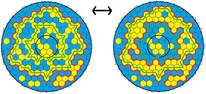
Figure 1: A sketch of the color switching trick used in the proof of Proposition 2.4.

Proof.

The proof of the equation is essentially the same as that of (2.39) in [12] for critical FPP on $\mathbb{Z}^{2}$. For completeness, we give the proof for our setting. If $\rho(r,R)=0$, then there exists a blue path connecting $\partial B(R)$ and $\partial B(r)$, and we get $T^{\prime}(r,R)=0$. We assume $\rho(r,R)>0$ in the following.

First we show $T^{\prime}(r,R)\geq\rho(r,R)$. This inequality is trivial, since if there are $\rho$ disjoint yellow circuits surrounding 0 in $A(r,R)$, any path connecting the two boundary pieces of $A(r,R)$ must intersect these circuits.

Next we show the converse inequality, $T^{\prime}(r,R)\leq\rho(r,R)$. We shall construct a path $\gamma$ connecting $\partial B(R)$ and $\partial B(r)$ such that $T(\gamma)=\rho(r,R)$, which implies $T^{\prime}(r,R)\leq\rho(r,R)$ immediately. Let $D_{0}:=B(R)$. Take $\mathcal{C}_{1}$ the outermost yellow circuit surrounding 0 in $D_{0}$ and let $D_{1}$ be the component of $D_{0}\backslash\mathcal{C}_{1}$ that contains 0, then take $\mathcal{C}_{2}$ the outermost yellow circuit surrounding 0 in $D_{1}$ and let $D_{2}$ be the component of $D_{1}\backslash\mathcal{C}_{2}$ that contains 0, and so on. The process stops after $\rho=\rho(r,R)$ steps. It is easy to see that $\mathcal{C}_{k}\subset A(r,R)$ for $1\leq k\leq\rho$ and there exists no yellow circuit surrounding 0 in $D_{\rho}\backslash B(r)$. Thus we can take a blue path $\gamma_{\rho}$ connecting $\Delta B(r)$ and a site $v_{\rho}$ in $\mathcal{C}_{\rho}$ (note that $\gamma_{\rho}$ may be empty if $\mathcal{C}_{\rho}$ intersects $\Delta B(r)$, similar case may occur below), then a blue path $\gamma_{\rho-1}$ connecting $v_{\rho}$ and a site $v_{\rho-1}$ in $\mathcal{C}_{\rho-1}$ since $\mathcal{C}_{\rho}$ is the outermost yellow circuit in $D_{\rho-1}$, and so on. The process stops after $\rho+1$ steps, and $\gamma_{0}$ is a blue path connecting $v_{1}\in\mathcal{C}_{1}$ and the inner site boundary of $B(R)$. Let $\gamma=\gamma_{0}v_{1}\ldots\gamma_{\rho-1}v_{\rho}\gamma_{\rho}$. Clearly $\gamma$ connects $\partial B(R)$ and $\partial B(r)$ and $T(\gamma)=\rho(r,R)$.

We now turn to the proof of the second property. See Fig. 1 for an illustration of the following argument. Since $B(R)$ has monochromatic (blue) boundary condition, it is easy to see that $N(r,R)$ equals the maximal number of disjoint circuits $\mathcal{C}_{1}^{\prime},\mathcal{C}_{2}^{\prime},\ldots$ surrounding 0 in $A(r,R)$ with alternating colors (yellow, blue, yellow, blue, $\ldots$) and $\overline{\mathcal{C}_{1}^{\prime}}\supset\overline{\mathcal{C}_{2}^{\prime}}\supset\ldots$. For any fixed $n\in\mathbb{N}\cup\{0\}$, we shall construct a bijection between the sets $\{\omega:\rho(r,R)=n\}$ and $\{\omega^{\prime}:N(r,R)=n\}$. Given a configuration $\omega\in\{\rho(r,R)=n\}$, we construct a sequence of yellow circuits $\mathcal{C}_{1},\ldots,\mathcal{C}_{n}$ from outside to inside and a sequence of connected domains $D_{0},\ldots,D_{n}$ as in the proof of the first property. If $n$ is odd, we switch the colors of the sites in $D_{1}\backslash D_{2},\ldots,D_{n-2}\backslash D_{n-1},D_{n}$; if $n$ is even, we switch the colors of the sites in $D_{1}\backslash D_{2},\ldots,D_{n-1}\backslash D_{n}.$ Denote this transformation by $f_{n}$. Then $f_{n}(\omega)\in\{N(r,R)=n\}$. This can be seen as follows: When $n$ is odd, after the transformation $f_{n}$, the color of $\mathcal{C}_{1},\mathcal{C}_{3},\ldots,\mathcal{C}_{n}$ is invariant and the color of $\mathcal{C}_{2},\mathcal{C}_{4},\ldots,\mathcal{C}_{n-1}$ is switched to blue. Then we can find a cluster boundary loop surrounding 0 in each $D_{j}\backslash D_{j+1},0\leq j\leq n-1$. Furthermore, none of these domains has two such loops, otherwise it would produce a yellow circuit surrounding 0 between two successive circuits $\mathcal{C}_{j}$ and $\mathcal{C}_{j+1}$ or outside $\mathcal{C}_{1}$ in $D_{0}$ in the original configuration, which contradicts our construction. There does not exist cluster boundary loop surrounding 0 in $D_{n}\backslash B(r)$ since $\omega\in\{\rho(r,R)=n\}$. Hence, $f_{n}(\omega)\in\{N(r,R)=n\}$. The argument is similar when $n$ is even.

Given a configuration $\omega^{\prime}\in\{N(r,R)=n\}$, similarly as above, we let $D_{0}^{\prime}:=B(R)$, take $\mathcal{C}_{1}^{\prime}$ the outermost yellow circuit surrounding 0 in $D_{0}^{\prime}$ and let $D_{1}^{\prime}$ be the component of $D_{0}^{\prime}\backslash\mathcal{C}_{1}^{\prime}$ that contains 0, then take $\mathcal{C}_{2}^{\prime}$ the outermost blue circuit surrounding 0 in $D_{1}^{\prime}$ and let $D_{2}^{\prime}$ be the component of $D_{1}^{\prime}\backslash\mathcal{C}_{2}^{\prime}$ that contains 0, and so on. The process stops after $n$ steps. If $n$ is odd, we switch the colors of the sites in $D_{1}^{\prime}\backslash D_{2}^{\prime},\ldots,D_{n-2}^{\prime}\backslash D_{n-1}^{\prime},D_{n}^{\prime}$; if $n$ is even, we switch the colors of the sites in $D_{1}^{\prime}\backslash D_{2}^{\prime},\ldots,D_{n-1}^{\prime}\backslash D_{n}^{\prime}.$ Note that $\omega^{\prime}$ is transformed to $\omega\in\{\rho(r,R)=n\}$ and this transformation is just $f_{n}^{-1}$. This can be seen as follows: When $n$ is odd, after the transformation, the color of $\mathcal{C}_{1}^{\prime},\mathcal{C}_{3}^{\prime},\ldots,\mathcal{C}_{n}^{\prime}$ is invariant and the color of $\mathcal{C}_{2}^{\prime},\mathcal{C}_{4}^{\prime},\ldots,\mathcal{C}_{n-1}^{\prime}$ is switched to yellow, and $\mathcal{C}_{j}^{\prime}$ is the outermost yellow circuit surrounding 0 in $D_{j-1}^{\prime},1\leq j\leq n$. Furthermore, $\rho(r,R)=n$, otherwise it would produce more than $n$ cluster boundary loops surrounding 0 in $A(r,R)$ before the transformation. Therefore, this transformation is just $f_{n}^{-1}$ by the construction and the definition of $f_{n}$. The argument is similar when $n$ is even. Then the bijection $f_{n}$ between $\{\omega:\rho(r,R)=n\}$ and $\{\omega^{\prime}:N(r,R)=n\}$ is constructed for each $n\in\mathbb{N}\cup\{0\}$, which completes the proof since we use the uniform measure. ∎

The following lemma gives upper large deviation bound for $T^{\prime}(r,R)$:

Lemma 2.5 (Corollary 2.3 in [26]).

There exist constants $C_{1},C_{2}>0$ and $K>1$, such that for all $1\leq r<R$ and $x\geq K\log_{2}(R/r)$,

$$P[T^{\prime}(r,R)\geq x]\leq C_{1}\exp(-C_{2}x).$$

In this paper, $C,C_{1},C_{2},\ldots$ denote positive finite constants that may change from line to line according to the context.

3 Proofs of the main results

3.1 Scaling limits of annulus times

For $0<\epsilon<1$, denote by $N(\epsilon)$ the number of CLE₆ loops surrounding 0 in $\overline{\mathbb{D}}\backslash\overline{\mathbb{D}}_{\epsilon}$. Camia and Newman’s full scaling limit allows us to derive a scaling limit of $T^{\prime}(\rho r,\rho R)$ as $\rho\rightarrow\infty$:

Proposition 3.1.

Suppose $1\leq r<R,\rho>0$ and $k\in\mathbb{N}$. Assume that $B(\rho R)$ has monochromatic (blue) boundary condition. As $\rho\rightarrow\infty$, we have

$$T^{\prime}(\rho r,\rho R)\stackrel{{\scriptstyle d}}{{\longrightarrow}}N(r/R),$$ (10)

$$E[(T^{\prime}(\rho r,\rho R))^{k}]\rightarrow\mathbb{E}[(N(r/R))^{k}].$$ (11)

Proof.

Let

$$\mathcal{F}_{\rho} :=\mbox{the collection of cluster boundary loops surrounding 0 in $A(\rho r,\rho R)$}$$

$$~{}~{}~{}~{}~{}\mbox{scaled by $1/(\rho R)$},$$

$$\mathcal{F} :=\mbox{the collection of CLE${}_{6}$ loops surrounding 0 in $\overline{\mathbb{D}}\backslash\overline{\mathbb{D}}_{r/R}$}.$$

Define event

$$\mathcal{A}_{\epsilon,\rho}:=\{\exists\mathcal{L}\in\mathcal{F}_{\rho}\mbox{ such that }\mathcal{L}\cap(\mathbb{D}_{(1+\epsilon)r}\backslash\mathbb{D}_{(1-\epsilon)r})\neq\emptyset\}.$$

Assume that $\mathcal{A}_{\epsilon,\rho}$ holds and $\rho$ is large enough (depending on $\epsilon$). Then we have a polychromatic 3-arm event from a ball of radius $3\epsilon$ centered at a point $z\in\partial\mathbb{D}_{(1-\epsilon)r}$ to a distance of unit order in $\overline{\mathbb{D}}\backslash\mathbb{D}_{(1-\epsilon)r}$. For a fixed $z\in\partial\mathbb{D}_{(1-\epsilon)r}$, the corresponding 3-arm event happens with probability at most $O(\epsilon^{2})$ (see e.g. Lemma 6.8 in [23]). From this one easily obtains $P[\mathcal{A}_{\epsilon,\rho}]\leq O(\epsilon)$. Then Theorem 2.1 implies that $\mathcal{F}_{\rho}$ converges in distribution to $\mathcal{F}$ as $\rho\rightarrow\infty$. Because of the choice of topology, we can find coupled versions of $\mathcal{F}_{\rho}$ and $\mathcal{F}$ on the same probability space such that $\operatorname{dist}(\mathcal{F}_{\rho},\mathcal{F})\rightarrow 0$ a.s. as $\rho\rightarrow\infty$ (see e.g. Theorem 6.7 of [4], similar couplings were used in [5]).

Now let us show that for large $\rho$, with high probability the distance $\textrm{d}(\cdot,\cdot)$ between the loops in $\mathcal{F}_{\rho}$ is not very small. Define event

$$\mathcal{B}_{\epsilon,\rho}:=\{\exists\mathcal{L}_{1},\mathcal{L}_{2}\in\mathcal{F}_{\rho}\mbox{ such that }\textrm{d}(\mathcal{L}_{1},\mathcal{L}_{2})<\epsilon\}.$$

Assume that $\mathcal{B}_{\epsilon,\rho}$ holds and $\rho$ is large enough (depending on $\epsilon$). Suppose $\mathcal{L}_{2}$ is in the interior of $\mathcal{L}_{1}$. Note that the polychromatic half-plane 3-arm exponent $\beta_{3}$ is 2 and the polychromatic plane 6-arm exponent $\alpha_{6}$ is larger that 2 (see e.g. [16]). Let $0<\alpha<1-2/\alpha_{6}$ be a fixed number. If $\mathcal{L}_{1}$ comes $\epsilon^{\alpha}/2$-close to $\partial\mathbb{D}$, then we have a half-plane 3-arm event from a ball of radius $2\epsilon^{\alpha}$ centered on a point in $\partial\mathbb{D}$ to a distance of unit order in $\overline{\mathbb{D}}$; otherwise, we have a polychromatic plane 6-arm event from radius $\epsilon$ to $\epsilon^{\alpha}/2$ in $\overline{\mathbb{D}}$. So, the event $\mathcal{B}_{\epsilon,\rho}$ happens with probability at most $O(\epsilon^{-\alpha}\epsilon^{\alpha\beta_{3}}+\epsilon^{-2}\epsilon^{(1-\alpha)(\alpha_{6}+o(1))})=O(\epsilon^{\alpha}+\epsilon^{(1-\alpha)(\alpha_{6}+o(1))-2})$. This implies that in the above coupling, the number of loops in $\mathcal{F}_{\rho}$ converges in probability to the number of loops in $\mathcal{F}$ as $\rho\rightarrow\infty$. Then we get $N(\rho r,\rho R)\stackrel{{\scriptstyle d}}{{\longrightarrow}}N(r/R)$ immediately. From Proposition 2.4, we obtain (10). Lemma 2.5 and (10) imply (11). ∎

The key ingredient Theorem 2.2 enables us to obtain the following limit theorem for $N(\epsilon)$:

Proposition 3.2.

$$\lim_{\epsilon\rightarrow 0}\frac{\mathbb{E}[N(\epsilon)]}{\log(1/\epsilon)}=\frac{1}{2\sqrt{3}\pi},~{}~{}\lim_{\epsilon\rightarrow 0}\frac{N(\epsilon)}{\log(1/\epsilon)}=\frac{1}{2\sqrt{3}\pi}~{}~{}a.s.,$$ (12)

$$\lim_{\epsilon\rightarrow 0}\frac{\operatorname{Var}[N(\epsilon)]}{\log(1/\epsilon)}=\frac{2}{3\sqrt{3}\pi}-\frac{1}{2\pi^{2}}.$$ (13)

Proof.

From Proposition 1 in [17], we know that $\{B_{k}\}_{k\in\mathbb{N}}$ are i.i.d. random variables. It is clear that $S_{n}:=\sum_{k=1}^{n}B_{k}=-\log\operatorname{CR}(U_{n}),n\geq 1$ is a renewal process. We let $N_{t}:=\inf\{n:S_{n}>t\}$ denote the number of renewals in $[0,t]$. Schwarz Lemma and the Koebe $1/4$ Theorem (see e.g. Lemma 2.1 and Theorem 3.17 in [13]) imply that

$$\frac{\operatorname{CR}(U_{n})}{4}\leq\operatorname{dist}(0,\mathcal{L}_{n})\leq\operatorname{CR}(U_{n}).$$

Hence, $\operatorname{CR}(U_{N(\epsilon)})\geq\operatorname{dist}(0,\mathcal{L}_{N(\epsilon)})>\epsilon$ and $\operatorname{CR}(U_{N(\epsilon)+1})\leq 4\operatorname{dist}(0,\mathcal{L}_{N(\epsilon)+1})\leq 4\epsilon$. Then we have

$$N_{\log(1/(5\epsilon))}-1\leq N(\epsilon)<N_{\log(1/\epsilon)}.$$ (14)

Applying the elementary renewal theorem and law of large numbers for renewal processes (see e.g. (4.1) and (4.2) in Section 3.4 in [9]), we know

$$\lim_{t\rightarrow\infty}\frac{\mathbb{E}[N_{t}]}{t}\rightarrow\frac{1}{\mathbb{E}[B_{1}]},~{}~{}\lim_{t\rightarrow\infty}\frac{N_{t}}{t}\rightarrow\frac{1}{\mathbb{E}[B_{1}]}~{}~{}a.s.$$ (15)

Combining (8), (14) and (15), we obtain (12).

There is a variance analogue of the elementary renewal theorem, see e.g. (1.6) in [22]. From this we know

$$\lim_{t\rightarrow\infty}\frac{\operatorname{Var}[N_{t}]}{t}=\frac{\operatorname{Var}[B_{1}]}{(\mathbb{E}[B_{1}])^{3}}.$$ (16)

The triangle inequality for the norm $\|\cdot\|_{2}=\sqrt{\mathbb{E}[|\cdot|^{2}]}$ and (14) give

$$\left|\sqrt{\operatorname{Var}[N(\epsilon)]}-\sqrt{\operatorname{Var}[N_{\log(1/\epsilon)}]}\right| \leq\sqrt{\operatorname{Var}[N(\epsilon)-N_{\log(1/\epsilon)}]}$$

$$\leq\sqrt{\mathbb{E}[(N_{\log(1/\epsilon)}-N_{\log(1/(5\epsilon))}+1)^{2}]}.$$

It is easy to see that the number of renewals in each time interval of length $\log 5$ can be uniformly dominated by a positive random variable with an exponential tail. Therefore, there exists a constant $C>0$ such that for all $0<\epsilon<1$,

$$\left|\sqrt{\operatorname{Var}[N(\epsilon)]}-\sqrt{\operatorname{Var}[N_{\log(1/\epsilon)}]}\right|\leq C.$$

Combining this inequality, (16) and Corollary 2.3, we get (13). ∎

Remark.

In fact, if one uses second-order approximations to the expectation-time and variance-time curves for renewal processes (see e.g. (1.4) and the equation just above Section 1.5 in [22]) in the above proof, one obtains that there exists a constant $C>0$ such that for all $0<\epsilon<1$,

$$\left|\mathbb{E}[N(\epsilon)]-\frac{\log(1/\epsilon)}{2\sqrt{3}\pi}\right|\leq C,~{}~{}\left|\operatorname{Var}[N(\epsilon)]-\frac{\log(1/\epsilon)}{\frac{2}{3\sqrt{3}\pi}-\frac{1}{2\pi^{2}}}\right|\leq C.$$

We note that the first inequality above has been proved in [15] (see (3.8) in [15]).

3.2 Limit results for $c_{n}$ and $E[c_{n}]$

Recall that $c_{n}$ is the passage time from 0 to $\partial B(n)$. In order to prove our limit results for $c_{n}$ and $E[c_{n}]$, we need some lemmas. In [26], we proved the following result.

Lemma 3.3 (Lemma 2.5 in [26]).

$$\lim_{n\rightarrow\infty}\frac{c_{n}}{E[c_{n}]}=1~{}~{}a.s.$$

Lemma 2.5 together with RSW and FKG (see e.g. [24]), gives the following lemma. Note that (18) was first proved in [7].

Lemma 3.4.

There exist $C_{1},C_{2}>0$ such that for all $1\leq r\leq R/2$,

$$C_{1}\log(R/r)\leq E[T^{\prime}(r,R)]\leq C_{2}\log(R/r).$$ (17)

In particular, for all $n\geq 2$,

$$C_{1}\log n\leq E[c_{n}]\leq C_{2}\log n.$$ (18)

For $x\geq 0$, denote by $S_{x}$ the maximum number of disjoint yellow circuits that surround 0 and intersect with $\partial B(2^{x})$. Using RSW, FKG and BK inequality, it is easy to obtain the following result.

Lemma 3.5.

There exists a constant $C>0$, such that for all $x,t\geq 0$,

$$P[S_{x}\geq t]\leq\exp(-Ct).$$ (19)

Hence, there is a constant $C_{0}>0$ (independent of $x$), such that

$$E[S_{x}]\leq C_{0}.$$ (20)

Now we are ready to prove the limit result for $c_{n}$ and $E[c_{n}]$:

Proposition 3.6.

$$\lim_{n\rightarrow\infty}\frac{c_{n}}{\log n}=\frac{1}{2\sqrt{3}\pi}~{}~{}a.s.,$$ (21)

$$\lim_{n\rightarrow\infty}\frac{E[c_{n}]}{\log n}=\frac{1}{2\sqrt{3}\pi}.$$ (22)

Proof.

Note that Lemma 3.3 and (22) imply (21), so it suffices to show (22). We write $T_{k,j}:=T^{\prime}(2^{k(j-1)},2^{kj})$. By Proposition 2.4, for $k\in\mathbb{N}$ and $n\geq 2^{k}$, it is clear that

$$-1+\sum_{j=1}^{\lfloor\log_{2^{k}}n\rfloor}T_{k,j}\leq c_{n}\leq 1+\rho(1,n)\leq 1+\sum_{j=1}^{\lfloor\log_{2^{k}}n\rfloor+1}(T_{k,j}+S_{kj}).$$ (23)

Combining this with (17) and (20), we obtain that there exists $C_{1},C_{2}>0$ such that

$$-1+\sum_{j=1}^{\lfloor\log_{2^{k}}n\rfloor}E[T_{k,j}]\leq E[c_{n}]\leq C_{1}\log_{2^{k}}n+C_{2}k+\sum_{j=1}^{\lfloor\log_{2^{k}}n\rfloor}E[T_{k,j}].$$

This and (18) imply that for each $0<\epsilon<1$, there exists $k_{0}(\epsilon)>0$, such that for each $k\geq k_{0}$, for $n$ sufficiently large (depending on $k$),

$$1-\epsilon\leq\frac{\sum_{j=1}^{\lfloor\log_{2^{k}}n\rfloor}E[T_{k,j}]}{E[c_{n}]}\leq 1+\epsilon.$$ (24)

By the convergence of the Cesàro mean and (11), we obtain

$$\lim_{m\rightarrow\infty}\frac{\sum_{j=1}^{m}E[T_{k,j}]}{m}=E[N(1/2^{k})].$$ (25)

Then (22) follows from (12), (24) and (25):

$$\lim_{n\rightarrow\infty}\frac{E[c_{n}]}{\log n}=\lim_{k\rightarrow\infty}\lim_{n\rightarrow\infty}\frac{\sum_{j=1}^{\lfloor\log_{2^{k}}n\rfloor}E[T_{k,j}]}{\log n}=\lim_{k\rightarrow\infty}\frac{E[N(1/2^{k})]}{\log(2^{k})}=\frac{1}{2\sqrt{3}\pi}.$$

∎

3.3 Limit result for $\operatorname{Var}[c_{n}]$

The proof of the result relating to variance turns out to be more involved than that to expectation. We shall use the martingale approach in [12], with a modification by introducing an intermediate scale. Let us mention that an analogous martingale method was used in [25] to prove a CLT for winding angles of arms in 2D critical percolation. We start with some definitions.

For $j\in\mathbb{N}\cup\{0\}$, define annulus

$$A(j):=A(2^{j},2^{j+1}).$$

Furthermore, define

$$m(j):=\inf\{k\geq j:A(k)\mbox{ contains a blue circuit surrounding 0}\},$$

$$\mathcal{C}_{j}:=\mbox{the innermost blue circuit surrounding 0 in }A(m(j)),$$

$$\mathscr{F}_{j}:=\sigma\mbox{-field generated by }\{t(v):v\in\overline{\mathcal{C}}_{j}\}.$$

For all $j\geq 1$, denote by $\mathcal{C}_{-j}$ the origin and by $\mathscr{F}_{-j}$ the trivial $\sigma$-field. For $k,q\in\mathbb{N}$, write

$$T(0,\mathcal{C}_{kq})-E[T(0,\mathcal{C}_{kq})]=\sum_{j=0}^{q}\left(E[T(0,\mathcal{C}_{kq})|\mathscr{F}_{kj}]-E[T(0,\mathcal{C}_{kq})|\mathscr{F}_{k(j-1)}]\right):=\sum_{j=0}^{q}\Delta_{k,j}.$$

Then $\{\Delta_{k,j}\}_{0\leq j\leq q}$ is an $\mathscr{F}_{kj}$-martingale increment sequence. Hence,

$$\operatorname{Var}[T(0,\mathcal{C}_{kq})]=\sum_{j=0}^{q}E[\Delta_{k,j}^{2}].$$ (26)

We will use this sum to estimate $\operatorname{Var}[c_{n}]$.

Let $(\Omega^{\prime},\mathscr{F}^{\prime},P^{\prime})$ be a copy of $(\Omega,\mathscr{F},P)$. Denote by $E^{\prime}$ the expectation with respect to $P^{\prime}$, and by $\omega^{\prime}$ a sample point in $\Omega^{\prime}$. Let $T(\cdot,\cdot)(\omega),m(j,\omega)$ and $\mathcal{C}_{j}(\omega)$ denote the quantities defined before, but with explicit dependence on $\omega$. Define $l(j,\omega,\omega^{\prime}):=m(m(j,\omega)+1,\omega^{\prime})$. We need the following results, which were proved in [12]. Note that (27) follows from RSW and FKG, and the proof of (28) is essentially the same as that of Lemma 2 in [12].

Lemma 3.7 ([12]).

(i) There exists $C>0$, such that for all $j,t\in\mathbb{N}$, we have

$$P[m(j)\geq j+t]\leq\exp(-Ct).$$ (27)

(ii) For $j\geq 0$ and $k\geq 1$, $\Delta_{k,j}$ does not depend on $q$. Furthermore,

$$\Delta_{k,j}(\omega)= T(\mathcal{C}_{k(j-1)}(\omega),\mathcal{C}_{kj}(\omega))(\omega)+E^{\prime}[T(\mathcal{C}_{kj}(\omega),\mathcal{C}_{l(kj,\omega,\omega^{\prime})}(\omega^{\prime}))(\omega^{\prime})]$$

$$-E^{\prime}[T(\mathcal{C}_{k(j-1)}(\omega),\mathcal{C}_{l(kj,\omega,\omega^{\prime})}(\omega^{\prime}))(\omega^{\prime})].$$ (28)

Next we bound the variances of $\Delta_{k,j}$ and $T(0,\mathcal{C}_{j})$.

Lemma 3.8.

There exist $C_{1},C_{2}>0$ such that for all $j,k\geq 1$,

$$C_{1}k\leq E[\Delta_{k,j}^{2}]\leq C_{2}k,$$ (29)

$$C_{1}j\leq\operatorname{Var}[T(0,\mathcal{C}_{j})]\leq C_{2}j.$$ (30)

Proof.

From (26), we know that (30) is just (2.32) in [12]. The proof of (2.32) in [12] implies that there exist universal $C_{1},C_{2}>0$ such that for all $n\in\mathbb{N}$,

$$C_{1}\leq E[\Delta_{1,n}^{2}]\leq C_{2}.$$

Since

$$E[\Delta_{k,j}^{2}]=\sum_{n=kj-k+1}^{kj}E[\Delta_{1,n}^{2}],$$

then (29) follows. ∎

The next lemma implies that for fixed $k$ and large $q$, if $2^{kq}\leq n\leq 2^{k(q+1)}$, the variance of $c_{n}$ is well approximated by that of $T(0,\mathcal{C}_{kq})$.

Lemma 3.9.

There exists $C>0$, such that for all $q\geq k\geq 1$ and $2^{kq}\leq n\leq 2^{k(q+1)}$,

$$\left|\operatorname{Var}[T(0,\mathcal{C}_{kq})]-\operatorname{Var}[c_{n}]\right|\leq C\sqrt{q}k^{3/2}.$$ (31)

Furthermore, there exist $C_{1},C_{2}>0$ such that for all $n\geq 2$,

$$C_{1}\log n\leq\operatorname{Var}[c_{n}]\leq C_{2}\log n.$$ (32)

Proof.

Recall that $S_{j}$ denotes the maximum number of disjoint yellow circuits that surround 0 and intersect with $\partial B(2^{j})$. Applying Lemma 2.5, (19) and (27), there exist $C_{1},C_{2}>0$, such that for all $x\geq 3Kk$, where $K$ is from Lemma 2.5, we have

$$P[|T(0,\mathcal{C}_{kq})-c_{n}|\geq x]$$

$$\leq P[m(kq)\geq kq+\lfloor x/(2K)\rfloor]+P[T^{\prime}(2^{kq},2^{kq+\lfloor x/(2K)\rfloor})\geq x/2]+P[S_{kq}\geq x/2]$$

$$\leq C_{1}\exp(-C_{2}x).$$

Then there is a universal $C_{3}>0$, such that

$$E[|T(0,\mathcal{C}_{kq})-c_{n}|^{2}]\leq C_{3}k^{2}.$$

Therefore, by the triangle inequality for the norm $\|\cdot\|_{2}=\sqrt{E[|\cdot|^{2}]}$, we have

$$\left|\sqrt{\operatorname{Var}[T(0,\mathcal{C}_{kq})]}-\sqrt{\operatorname{Var}[c_{n}]}\right| \leq\sqrt{\operatorname{Var}[T(0,\mathcal{C}_{kq})-c_{n}]}\leq\sqrt{C_{3}}k.$$

Combining this and (30) gives (31).

(32) follows from (30) and (31) immediately. ∎

Recall that $T_{k,j}:=T^{\prime}(2^{k(j-1)},2^{kj})$. The following is a key estimate for $T_{k,j}$, which says that for large $k$, the variance of $T_{k,j}$ is well approximated by that of $\Delta_{k,j}$ (since $E[\Delta_{k,j}^{2}]\asymp k$, from (29)).

Lemma 3.10.

There exists a constant $C>1$, such that for all $k,j\in\mathbb{N}$,

$$\left|\operatorname{Var}[T_{k,j}]-E[\Delta_{k,j}^{2}]\right|\leq C\sqrt{k}.$$

Proof.

We claim that there exist universal constants $C_{1},C_{2}>0$ such that for all $k,j\in\mathbb{N}$ and $x>0$,

$$P[|T_{k,j}-E[T_{k,j}]-\Delta_{k,j}|\geq x]\leq C_{1}\exp(-C_{2}x).$$ (33)

Therefore, there is a $C_{3}>0$ such that

$$E[|T_{k,j}-E[T_{k,j}]-\Delta_{k,j}|^{2}]\leq C_{3}.$$

Then we obtain

$$|\{\operatorname{Var}[T_{k,j}]\}^{1/2}-\{\operatorname{Var}[\Delta_{k,j}]\}^{1/2}|\leq\{E[|T_{k,j}-E[T_{k,j}]-\Delta_{k,j}|^{2}]\}^{1/2}\leq\sqrt{C_{3}}.$$

This and (29) imply the desired result:

$$\left|\operatorname{Var}[T_{k,j}]-E[\Delta_{k,j}^{2}]\right|\leq 2\sqrt{C_{3}E[\Delta_{k,j}^{2}]}+C_{3}\leq C\sqrt{k}.$$

We now show our claim (33). By (28), proving (33) boils down to proving that there exist $C_{4},C_{5},C_{6},C_{7}>0$ such that

$$P[|T_{k,j}-T(\mathcal{C}_{k(j-1)},\mathcal{C}_{kj})|\geq x]\leq C_{4}\exp(-C_{5}x),$$ (34)

$$P[|E[T_{k,j}]+E^{\prime}[T(\mathcal{C}_{kj}(\omega),\mathcal{C}_{l(kj,\omega,\omega^{\prime})}(\omega^{\prime}))]-E^{\prime}[T(\mathcal{C}_{k(j-1)}(\omega),\mathcal{C}_{l(kj,\omega,\omega^{\prime})}(\omega^{\prime}))]|\geq x]$$

$$~{}~{}\leq C_{6}\exp(-C_{7}x).$$ (35)

We first prove (34). Let $C_{8}=1/(4K)$, where $K$ is from Lemma 2.5. There exist $C_{9},C_{10},C_{11},C_{12}>0$ such that if $0<x\leq k/C_{8}$,

$$P[|T_{k,j}-T(\mathcal{C}_{k(j-1)},\mathcal{C}_{kj})|\geq x]$$

$$\leq P[m(k(j-1))\geq k(j-1)+\lfloor C_{8}x\rfloor]+P[m(kj-\lfloor C_{8}x\rfloor)\geq kj]+P[m(kj)\geq kj+\lfloor C_{8}x\rfloor]$$

$$~{}~{}~{}~{}+P[T^{\prime}(2^{k(j-1)},2^{k(j-1)+\lfloor C_{8}x\rfloor})\geq x/2]+P[T^{\prime}(2^{kj-\lfloor C_{8}x\rfloor},2^{kj+\lfloor C_{8}x\rfloor})\geq x/2]$$

$$\leq 3C_{9}\exp(-C_{10}x)+2C_{11}\exp(-C_{12}x)~{}~{}\mbox{ by (\ref{e27}) and Lemma \ref{l10}};$$

if $x\geq k/C_{8}$,

$$P[|T_{k,j}-T(\mathcal{C}_{k(j-1)},\mathcal{C}_{kj})|\geq x]$$

$$~{}~{}~{}~{}\leq P[m(kj)\geq kj+\lfloor C_{8}x\rfloor]+P[T^{\prime}(2^{k(j-1)},2^{kj+\lfloor C_{8}x\rfloor})\geq x]$$

$$~{}~{}~{}~{}\leq C_{9}\exp(-C_{10}x)+C_{11}\exp(-C_{12}x)~{}~{}\mbox{ by (\ref{e27}) and Lemma \ref{l10}}.$$

Then (34) follows immediately.

Now let us show (35), which follows from the two inequalities below:

$$E^{\prime}[T(\mathcal{C}_{kj}(\omega),\mathcal{C}_{l(kj,\omega,\omega^{\prime})}(\omega^{\prime}))]\leq C_{13}~{}~{}a.s.,$$ (36)

$$P[|E^{\prime}[T_{k,j}(\omega^{\prime})]-E^{\prime}[T(\mathcal{C}_{k(j-1)}(\omega),\mathcal{C}_{l(kj,\omega,\omega^{\prime})}(\omega^{\prime}))]|\geq x]\leq C_{14}\exp(-C_{15}x),$$ (37)

where $C_{13},C_{14},C_{15}>0$ are universal constants. Using (27) and Lemma 2.5 again, we know there exist $C_{16},C_{17}>0$ such that for all $\mathcal{C}_{kj}(\omega)$,

$$P^{\prime}[T(\mathcal{C}_{kj}(\omega),\mathcal{C}_{l(kj,\omega,\omega^{\prime})}(\omega^{\prime}))\geq x]$$

$$~{}~{}~{}~{}\leq P^{\prime}[l(kj,\omega,\omega^{\prime})\geq m(kj,\omega)+\lfloor C_{8}x\rfloor]+P^{\prime}[T^{\prime}(2^{m(kj,\omega)},2^{m(kj,\omega)+\lfloor C_{8}x\rfloor})\geq x]$$

$$~{}~{}~{}~{}\leq C_{16}\exp(-C_{17}x),$$

which implies (36).

It remains to show (37). Similarly to the proof of (34), one can show that there exist $C_{18},C_{19}>0$, such that

$$P^{\prime}[|T_{m(k(j-1),\omega),m(kj,\omega)+1}(\omega^{\prime})-T(\mathcal{C}_{k(j-1)}(\omega),\mathcal{C}_{l(kj,\omega,\omega^{\prime})}(\omega^{\prime}))|\geq x]\leq C_{18}\exp(-C_{19}x),$$

which implies that there is a universal $C_{20}>0$, such that

$$\left|E^{\prime}[T_{m(k(j-1),\omega),m(kj,\omega)+1}(\omega^{\prime})]-E^{\prime}[T(\mathcal{C}_{k(j-1)}(\omega),\mathcal{C}_{l(kj,\omega,\omega^{\prime})}(\omega^{\prime}))]\right|\leq C_{20}.$$

From this proving (37) boils down to proving that there are $C_{21},C_{22}>0$ such that

$$P[E^{\prime}[T_{k,j}(\omega^{\prime})]-E^{\prime}[T_{m(k(j-1),\omega),m(kj,\omega)+1}(\omega^{\prime})]\geq x]\leq C_{21}\exp(-C_{22}x).$$ (38)

Combining (17) and (20) gives that there exists $C_{24}>0$, such that for all $x\geq 1$ and $j\geq 0$,

$$E[T^{\prime}(2^{j},2^{j+x+1})+S_{j}+S_{j+x+1}]\leq x/(2C_{24}).$$ (39)

Then, using (39) and (27), we get that there exist $C_{25},C_{26}>0$ such that if $1/C_{24}\leq x\leq k/C_{24}$,

$$P[|E^{\prime}[T_{k,j}(\omega^{\prime})]-E^{\prime}[T_{m(k(j-1),\omega),m(kj,\omega)+1}(\omega^{\prime})]|\geq x]$$

$$~{}~{}~{}~{}\leq P[m(k(j-1))\geq k(j-1)+\lfloor C_{24}x\rfloor]+P[m(kj)\geq kj+\lfloor C_{24}x\rfloor]$$

$$~{}~{}~{}~{}~{}~{}~{}~{}~{}+P[E^{\prime}[T^{\prime}(2^{k(j-1)},2^{k(j-1)+\lfloor C_{24}x\rfloor+1})+S_{k(j-1)+\lfloor C_{24}x\rfloor+1}]\geq x]$$

$$~{}~{}~{}~{}~{}~{}~{}~{}~{}+P[E^{\prime}[T^{\prime}(2^{kj},2^{kj+\lfloor C_{24}x\rfloor+1})+S_{kj}]\geq x]$$

$$~{}~{}~{}~{}\leq C_{25}\exp(-C_{26}x)\mbox{ (note that the last two terms above equal 0});$$

if $x\geq k/C_{24}$,

$$P[|E^{\prime}[T_{k,j}(\omega^{\prime})]-E^{\prime}[T_{m(k(j-1),\omega),m(kj,\omega)+1}(\omega^{\prime})]|\geq x]$$

$$\leq P[m(kj)\geq kj+\lfloor C_{24}x\rfloor]+P[E^{\prime}[T^{\prime}(2^{k(j-1)},2^{kj+\lfloor C_{24}x\rfloor+1})]\geq x]\leq C_{25}\exp(-C_{26}x).$$

Then (38) follows immediately, which completes the proof. ∎

We are now ready to prove the limit result for $\operatorname{Var}[c_{n}]$:

Proposition 3.11.

$$\lim_{n\rightarrow\infty}\frac{\operatorname{Var}[c_{n}]}{\log n}=\frac{2}{3\sqrt{3}\pi}-\frac{1}{2\pi^{2}}.$$

Proof.

Applying Lemma 3.10, we have

$$\left|\operatorname{Var}[T(0,\mathcal{C}_{kq})]-\sum_{j=1}^{q}\operatorname{Var}[T_{k,j}]\right|\leq Cq\sqrt{k}+1,$$ (40)

where $C$ is from Lemma 3.10. By the convergence of the Cesàro mean and (11), we obtain

$$\lim_{q\rightarrow\infty}\frac{\sum_{j=1}^{q}\operatorname{Var}[T_{k,j}]}{q}=\operatorname{Var}[N(1/2^{k})].$$ (41)

Recall the choice $q=\lfloor\log_{2^{k}}n\rfloor$. Combining (13), (31), (32), (40) and (41) gives the desired result:

$$\lim_{n\rightarrow\infty}\frac{\operatorname{Var}[c_{n}]}{\log n}=\lim_{k\rightarrow\infty}\lim_{n\rightarrow\infty}\frac{\sum_{j=1}^{\lfloor\log_{2^{k}}n\rfloor}\operatorname{Var}[T_{k,j}]}{\log n}=\lim_{k\rightarrow\infty}\frac{\operatorname{Var}[N(1/2^{k})]}{\log(2^{k})}=\frac{2}{3\sqrt{3}\pi}-\frac{1}{2\pi^{2}}.$$

∎

3.4 Proofs of Theorem 1.1 and Corollary 1.2

Proof of Theorem 1.1.

The proof of Theorem 1.1 in [26], together with Proposition 3.6, implies (1) and (4) immediately.

By Lemma 2.5, (19) and (27), there exist $C_{1},C_{2}>0$, such that for all $2^{q}\leq n<2^{q+1}$, $x\geq 4K$, where $K$ is from Lemma 2.5, we have

$$P[b_{0,n}-c_{n}\geq x]$$

$$\leq P[T(0,\mathcal{C}_{q+1})-c_{2^{q}}\geq x]$$

$$\leq P[m(q+1)\geq q+\lfloor x/(2K)\rfloor]+P[T^{\prime}(2^{q},2^{q+\lfloor x/(2K)\rfloor})\geq x/2]+P[S_{q}\geq x/2]$$

$$\leq C_{1}\exp(-C_{2}x).$$

Then there is a universal $C_{3}>0$, such that

$$E[|b_{0,n}-c_{n}|]\leq C_{3},~{}~{}E[|b_{0,n}-c_{n}|^{2}]\leq C_{3}.$$ (42)

Then (2) follows from (22) and (42).

By (32) and (42), one easily obtains that there exists $C_{4}>0$ such that

$$|\operatorname{Var}[b_{0,n}]-\operatorname{Var}[c_{n}]|\leq C_{4}\sqrt{\log n}.$$

Then (3) follows from this and Proposition 3.11.

For $z\in A(2^{q},2^{q+1})$ and $q\geq 2$, define

$$Y(z):=T(0,\partial B(2^{q-1}))+T(z,\partial B(z,2^{q-1})).$$

It is obvious that $T(0,z)\geq Y(z)$ and

$$T(0,z)-Y(z)\leq|T(0,\mathcal{C}_{q+2})-T(0,\partial B(2^{q-1}))|+|T(z,\mathcal{C}_{q+2})-T(z,\partial B(z,2^{q-1}))|.$$

Using this inequality, similarly to the above argument, one can show that there is a universal $C_{5}>0$ such that

$$E[|T(0,z)-Y(z)|]\leq C_{5},~{}~{}E[|T(0,z)-Y(z)|^{2}]\leq C_{5},$$ (43)

see the proofs of Corollary 5.11 and 5.12 in [8]. Combining (22) and (43) gives (5) immediately. By (32) and (43) and using the triangle inequality for the norm $\|\cdot\|_{2}$, there exist universal $C_{6}>0$ such that

$$|\operatorname{Var}[T(0,z)]-2\operatorname{Var}[c_{2^{q-1}}]|\leq C_{6}\sqrt{q}.$$

Then we derive (6) from this and Proposition 3.11, finishing the proof. ∎

Proof of Corollary 1.2.

Using the Theorem in [12], one can derive the following result easily: As $n\rightarrow\infty$,

$$\frac{b_{0,n}-E[b_{0,n}]}{\sqrt{\operatorname{Var}[b_{0,n}]}}\stackrel{{\scriptstyle d}}{{\longrightarrow}}N(0,1),$$ (44)

$$\frac{T(0,nu)-E[T(0,nu)]}{\sqrt{\operatorname{Var}[T(0,nu)]}}\stackrel{{\scriptstyle d}}{{\longrightarrow}}N(0,1).$$ (45)

Note that (45) is a particular case of Corollary 5.13 in [8], and the proof of (44) is similar to that of (45). Corollary 1.2 follows from (44), (45) and Theorem 1.1 immediately. ∎

4 A discussion on the limit shape

Since there is a “shape theorem” for general non-critical FPP (see e.g. [3]), it is natural to ask if there is an analogous result for critical FPP. For that purpose, we view the sites of $\mathbb{V}$ as hexagons, and define $W(n):=\{v\in\mathbb{V}:T(0,v)\leq n\}$ for $n\in\mathbb{N}$. Unlike the non-critical case, there are “large holes” in $W(n)$, and the geometry of $W(n)$ is not easy to analyze. Instead, it would be easier to deal with the set $\overline{W}(n)$ obtained from $W(n)$ by filling in the holes. That is, $\overline{W}(n)$ is the closed set surrounded by the outer boundary of $W(n)$. We shall discuss the limit boundary of $\overline{W}(n)$ below.

Similarly to the proof of Proposition 2.4, we inductively define the $n$-th innermost disjoint yellow circuit $\mathcal{C}_{n}$ surrounding 0. For simplicity, if the hexagon centered at 0 is yellow, we also call it the first innermost circuit surrounding 0. Let $\mathcal{C}_{n}^{*}:=\mathcal{C}_{n}\cup$ blue clusters which touch $\mathcal{C}_{n}$. Observe that $\partial\overline{W}(n)$ is equal to the outer boundary of $\mathcal{C}_{n}^{*}$. By a color switching trick one obtains that $\partial\overline{W}(n)$ is equal in distribution to the $n$-th innermost cluster boundary loop $\mathcal{L}_{n}$ surrounding 0. Thus, it is expected that as $n\rightarrow\infty$, the limit boundary of $\overline{W}(n)$ under appropriate scaling has the same distribution as a “typical” loop of full-plane CLE₆. Note that $\overline{W}(n)$ grows approximately exponentially as time passes.

In [11], Kemppainen and Werner proved the invariance of full-plane CLE_κ under the inversion $z\mapsto 1/z$ for $0<\kappa\leq 4$. Although the analogous result has not been proved for the case $4<\kappa<8$, Miller and Sheffield [14] proved the time-reversal symmetry of whole-plane SLE_κ for $\kappa\in(0,8]$. To establish the following statement, for a loop $\mathcal{L}$ that surrounds 0, we let $R_{in}(\mathcal{L}):=\operatorname{dist}(0,\mathcal{L})$ denote the inner radius of $\mathcal{L}$ and let $R_{out}(\mathcal{L}):=\inf\{r:\overline{\mathbb{D}}_{r}\supset\mathcal{L}\}$ denote the outer radius of $\mathcal{L}$. By the argument above, it is expected that the following statement holds: As $n\rightarrow\infty$, the distributions of $\partial\overline{W}(n)/R_{in}(\partial\overline{W}(n))$ and $\partial\overline{W}(n)/R_{out}(\partial\overline{W}(n))$ converge, and we denote the two limit distributions by $\mu_{in}$ and $\mu_{out}$, respectively. Furthermore, $\mu_{out}$ is the image of $\mu_{in}$ under $z\mapsto 1/z$.

References

- [1]
- [2] Aizenman, M., Duplantier, B., Aharony, A.: Path crossing exponents and the external perimeter in 2D percolation. Phys. Rev. Let. 83, 1359–1362 (1999)
- [3] Auffinger, A., Damron, M., Hanson, J.: 50 years of first passage percolation. arXiv:1511.03262 (2016)
- [4] Billingsley, P.: Convergence of probability measures. Second Edition. Wiley Series in Probability and Statistics: Probability and Statistics. John Wiley Sons Inc., New York.
- [5] Camia, F., Newman, C.M.: Critical percolation: the full scaling limit. Commun. Math. Phys. 268, 1–38 (2006)
- [6] Camia, F., Newman, C.M.: SLE6 and CLE6 from critical percolation. In Pinsky, M. and Birnir, B. (eds) Probability, geometry and integrable systems, MSRI Publications, Volume 55, Cambridge University Press, New York, pp. 103–130 (2008)
- [7] Chayes, J.T., Chayes, L., Durrett, R.: Critical behavior of two-dimensional first passage time. J. Stat. Phys. 45, 933–951 (1986)
- [8] Damron, M., Lam, W.-K., Wang, W.: Asymptotics for 2D critical first passage percolation. arXiv:1505.07544 (2015) To appear in Annals of Probability.
- [9] Durrett, R.: Probability: Theory and Examples. Third Edition, Belmont CA: Duxbury Advanced Series (2004)
- [10] Grimmett, G., Kesten, H.: Percolation since Saint-Flour. In Percolation at Saint-Flour. Springer-Verlag, Heidelberg. (2012)
- [11] Kemppainen, A., Werner, W.: The nested simple conformal loop ensembles in the Riemann sphere. Probab. Theory Relat. Fields 165, 835–866 (2016)
- [12] Kesten, H., Zhang, Y.: A central limit theorem for “critical” first-passage percolation in two-dimensions. Probab. Theory Relat. Fields. 107, 137–160 (1997)
- [13] Lawler, G.F.: Conformally invariant processes in the plane. Amer. Math. Soc. (2005)
- [14] Miller, J., Sheffield, S.: Imaginary geometry IV: interior rays, whole-plane reversibility, and space-filling trees. arXiv:1302.4738 (2013)
- [15] Miller, J., Watson, S.S., Wilson, D.B.: The conformal loop ensemble nesting field. Probab. Theory Relat. Fields 163, 769–801 (2015)
- [16] Nolin, P.: Near critical percolation in two-dimensions. Electron. J. Probab. 13, 1562–1623 (2008)
- [17] Schramm, O., Sheffield, S., Wilson, D.B.: Conformal radii for conformal loop ensembles. Commun. Math. Phys. 288, 43–53 (2009)
- [18] Sheffield, S.: Exploration trees and conformal loop ensembles. Duke Math. J. 147, 79–129 (2009)
- [19] Sheffield S., Werner W.: Conformal loop ensembles: the Markovian characterization and the loop-soup construction. Ann. Math. 176, 1827–1917 (2012)
- [20] Smirnov, S.: Critical percolation in the plane: conformal invariance, Cardy s formula, scaling limits. C. R. Acad. Sci. Paris Sér. I Math. 333 no. 3, 239–244 (2001)
- [21] Smirnov, S., Werner, W.: Critical exponents for two-dimensional percolation. Math. Res. Lett. 8, 729–744 (2001)
- [22] Smith, W.L.: Renewal theory and its ramifications. Journal of the Royal Statistical Society. Series B (Methodological), Vol. 20, No. 2, 243–302 (1958)
- [23] Sun, N.: Conformally invariant scaling limits in planar critical percolation. Probab. Surveys 8, 155–209 (2011)
- [24] Werner, W.: Lectures on two-dimensional critical percolation. In: Statistical mechanics. IAS/Park City Math. Ser., Vol.16. Amer. Math. Soc., Providence, RI, 297–360 (2009)
- [25] Yao, C.-L.: A CLT for winding angles of the arms for critical planar percolation. Electron. J. Probab. 18, no. 85, 1–20 (2013)
- [26] Yao, C.-L.: Law of large numbers for critical first-passage percolation on the triangular lattice. Electron. Commun. Probab. 19, no. 18, 1–14 (2014)