Towards Quantum Simulation of Chemical Dynamics with Prethreshold Superconducting Qubits

Abstract

The single excitation subspace (SES) method for universal quantum simulation is investigated for a number of diatomic molecular collision complexes. Assuming a system of $n$ tunably-coupled, and fully-connected superconducting qubits, computations are performed in the $n$-dimensional SES which maps directly to an $n$-channel collision problem within a diabatic molecular wave function representation. Here we outline the approach on a classical computer to solve the time-dependent Schrödinger equation in an $n$-dimensional molecular basis - the so-called semiclassical molecular-orbital close-coupling (SCMOCC) method - and extend the treatment beyond the straight-line, constant-velocity approximation which is restricted to large kinetic energies ($\gtrsim 0.1$ keV/u). We explore various multichannel potential averaging schemes and an Ehrenfest symmetrization approach to allow for the application of the SCMOCC method to much lower collision energies (approaching 1 eV/u). In addition, a computational efficiency study for various propagators is performed to speed-up the calculations on classical computers. These computations are repeated for the simulation of the SES approach assuming typical parameters for realistic pretheshold superconducting quantum computing hardware. The feasibility of applying future SES processors to the quantum dynamics of large molecular collision systems is briefly discussed.

1 Introduction

While the field of chemical dynamics, including atomic and molecular collisional processes, has seen tremendous advances in theory, experiment, and computation over the past eight decades [1, 2, 3], computations which attempt to exactly solve the time-dependent (TD) or time-independent (TI) Schrödinger equation have been limited to consideration of only five [4] and four atoms [5], respectively. In the former case, solutions have been restricted to reactive processes, while the latter approach has focused on inelastic collisions, both incorporating full-dimensional dynamics on full-dimensional potential energy surfaces (PESs). Part of the reason for the dimensional limitation in such calculations is the need for significant computational resources, but more importantly the development of software and algorithms to treat large multidimensional systems has stagnated.

On the other hand, molecular electronic structure computations, or quantum chemistry, has seen rapid advances in both software and algorithm development with implementation on high performance distributed and shared-memory CPUs [2] as well as on new accelerator technologies such as graphical processing units (GPUs) [6]. Using the coupled-cluster singles and doubles (CCSD) approach [7], it is possible today to compute and analytically fit electronic potential and coupling surfaces for systems as large as 10 atoms [8]. As the number of internal degrees of freedom $d$ is $3N_{\rm atom}-6$, where $N_{\rm atom}$ is the number of atoms, this corresponds to a 24-dimensional surface. As an illustration, Figure 1 plots the PES dimension $d$ versus the number of atoms up to $N_{\rm atom}=10$, which is approximately the limit for the size of the largest molecular systems that can be both computed on a classical compute and fitted for dynamical studies. However, the region show in green displays the largest systems that can be computed, again on a classical computer, using full dimensional dynamics for TD reactive collisions. The region with $d>9$ can only be treated dynamically with quasi-classical methods, i.e. by solving Newton’s equations of motion for the heavy-particle trajectories. The situation for TI and quantum inelastic calculations is somewhat worse.

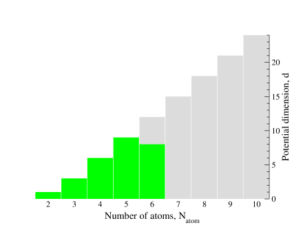
Figure 1: Status of time-dependent reactive calculations on classical computers in terms of the number of atoms $N_{\rm atom}$ and PES dimension $d$. Regime of possible quantum scattering calculations (green). Regime of available PESs which can currently only be treated by quasi-classical dynamical methods (grey).

Clearly computations of electronic structure have far out-paced the abilities of quantum dynamical calculations when the goal is to treat the problem nearly exact numerically and in full-dimension. Therefore, it appears that there is an opportunity to apply other, more novel approaches to advance quantum chemical dynamical studies and one might naturally turn to quantum computing/simulation. There has been considerable effort to explore the prospects of applying quantum simulation to the electronic structure problem [9, 10, 11], but investigations of chemical dynamics have been sparse to date [12, 13, 14]. The promising method of Kassal et al [14] applies a quantum gate-based logic approach, or digital quantum simulation (DQS). However, the DQS method requires 100s of gate operations and 100s of high-fidelity, fault-tolerant qubits. As the quantum simulation hardware has not advanced sufficiently to satisfy these resource requirements, we have proposed an alternative approach, the single excitation subspace (SES) method, which avoids the need for fault-tolerant devices using instead available prethreshold superconducting technology [15, 16]. While the SES method may not be scalable, it can solve a time-dependent, real, symmetric quantum Hamiltonian of dimension $n\times n$ using $n$ qubits with a quantum computation time that is independent of $n$ for a single run. However, an SES computer must be fully connected requiring $n(n-1)/2$ tunable couplers with $n$ also corresponding to the number of diabatic molecular channels in the collision problem to be simulated. The feasibility of the approach was outlined in Geller et al [16] for the simple, but well-studied $n=3$ Na+He electronic excitation problem. Here we extend that study to i) ion-atom charge exchange systems with $n$ as large as ten, ii) improve the trajectory calculation from the standard straight line, constant velocity approximation to explicitly solving for the relative velocity for a range of multichannel potential averaging schemes, and iii) apply the Ehrenfest symmetrization approach to correct for the loss of detail-balance due to potential averaging, with the latter two topics allowing for the classical calculations and SES simulations to be extended to low collision energies. iv) To allow for a future classical-quantum resource comparison, a TD propagator study is carried out to find the most efficient classical computational approach and v) we end by speculating on the prospects of large-scale SES device applications to large, chemically interesting reactions not feasible on today’s high performance computing platforms.

2 Molecular Collisions on a Classical Computer: Establishing Benchmarks

While there are a variety of approaches to attack atomic and molecular collision problems on a classical computer, the one that is most relevant to the SES method is the semiclassical molecular-orbital close-coupling (SCMOCC) approach. In the SCMOCC method, the TD Schrödinger equation is given by

$$i\frac{\partial\psi(\vec{r},t|R)}{\partial t}=h(\vec{r},t|R)\psi(\vec{r},t|R),$$ (1)

where $h(\vec{r},t|R)$ is the system Hamiltonian, $R$ the internuclear distance, $\vec{r}$ the collection of electronic (internal) coordinates, and $t$ the collision time [17]. The Hamiltonian is given by

$$h(\vec{r},t|R)=H_{\rm int}(\vec{r})+V(R(t),\vec{r})$$ (2)

and the system wave function $\psi(\vec{r},t|R)$ is expanded in a molecular basis by

$$\psi(\vec{r},t|R)=\sum_{i}^{n}a_{i}(t|R)\phi_{i}(\vec{r})$$ (3)

with $n$ the size of the basis or total number of channels. The asymptotic states are defined by the TI Schrödinger equation

$$H_{\rm int}(\vec{r})\phi_{i}(\vec{r})=E_{i}\phi_{i}(\vec{r})$$ (4)

resulting in $n$ coupled equations for the expansion coefficients

$$i\frac{da_{i}(t|R)}{dt}=\sum_{j}^{n}V_{ij}(t|R)a_{j}(t|R)$$ (5)

with $V_{ij}$ the potential matrix in the basis of states $\phi_{i}$

$$V_{ij}(t|R)=\bigl{<}\phi_{i}|V(R(t),\vec{r})|\phi_{j}\bigr{>}.$$ (6)

In the Born-Oppenheimer approximation, $V_{ij}$ are the usual electronic potentials which are diagonal in the adiabatic representation, and non-diagonal, but real and symmetric in the diabatic representation applied here.

In a semiclassical approach, quantum probabilities are propagated with time. For a given trajectory with initial asymptotic speed $v_{0}$ and impact parameter $b$ starting at a collision time $t\rightarrow-\infty$, the final probability for a transition from initial channel $i$ to final channel $f$ as $t\rightarrow\infty$ is

$$P_{if}(v_{0},b,t\rightarrow\infty)=P^{\infty}_{if}(v_{0},b)=|a_{f}(t\rightarrow\infty)|^{2},$$ (7)

with the initial condition

$$a_{i}(t\rightarrow-\infty)=\delta_{ij}$$ (8)

for a collision system with $n$ channels. At any time, unitarity must be satisfied, so that

$$\sum_{j=1}^{n}P_{ij}(v_{0},b,t)=1.$$ (9)

After performing the propagation for a large number of impact parameters over the range $b>0$ to $b_{\rm max}$, the integral cross section at a given initial speed $v_{0}$ is given by

$$\sigma_{if}(v_{0})=2\pi\int^{b_{\rm max}}_{0}P^{\infty}_{if}(v_{0},b)bdb,$$ (10)

where for

$$b>b_{\rm max},~{}~{}~{}~{}P^{\infty}_{if}(v_{0},b)\rightarrow 0~{}~{}~{}{\rm and}~{}~{}~{}P^{\infty}_{ii}(v_{0},b)\rightarrow 1.$$ (11)

As test cases, we expand upon our earlier atom-atom $n=3$ Na+He electronic excitation work [16] and consider larger ($n=3-10$) ion-atom charge exchange collisions. See Refs. [16, 18] for details on the Na-He potential matrix and straight line trajectory calculations.

2.1 Si³⁺ + He

The charge exchange process

$${\rm Si}^{3+}(3s~{}^{2}S)+{\rm He}(1s^{2}~{}^{1}S) \rightarrow {\rm Si}^{2+}(3s^{2}~{}^{1}S)+{\rm He}^{+}(1s~{}^{2}S),$$ (12)

$$\rightarrow {\rm Si}^{2+}(3s3p~{}^{3}P^{o})+{\rm He}^{+}(1s~{}^{2}S),$$ (13)

$$\rightarrow {\rm Si}^{2+}(3s3p~{}^{1}P^{o})+{\rm He}^{+}(1s~{}^{2}S).$$ (14)

was studied by Stancil et al [19] using a TI quantum molecular-orbital close-coupling (QMOCC) approach [20, 21]. It is an $n=5$ channel case which also includes excitation to Si³⁺($3p~{}^{2}P^{0}$). The diabatic PESs, $V_{ii}$, are displayed in Fig. 2, while the off-diagonal coupling elements $V_{ij}$ can be found in Ref. [19].

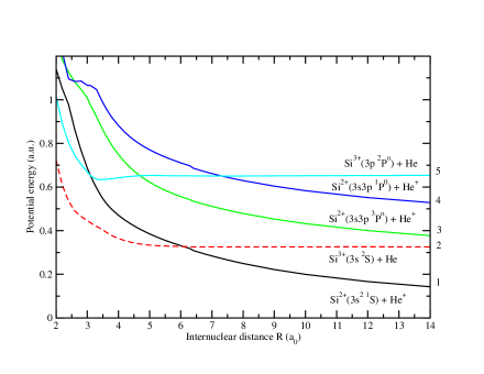
Figure 2: Diabatic potentials for the SiHe³⁺ system from Ref. [19]. Channel numbers are indicated on the right side. The initial channel in the current simulations is taken to be 2 or 1.

However, we begin by considering just the first three channels (i.e., $n=3$) with probabilities versus collision time given in Fig. 3 for $v_{0}=0.5$ a.u. and $b=0.6$ a₀. The dominant capture channel is to the exoergic channel 1. A $n=5$ calculation is shown in Fig. 4 with the ground state being the initial channel. Other probability evolution examples for various $v_{0}$ and $b$ and for $n=4$ and $n=5$ simulations are given in the Supplement.

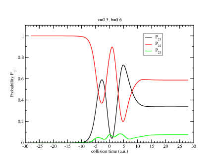
Figure 3: The Si³⁺ + He probabilities as a function of collision time for the elastic ($2\rightarrow 2$) and charge exchange transitions ($2\rightarrow 1$ and $2\rightarrow 3$). $n=3$ channel case with $b=0.6$ a₀ and $v_{0}=0.5$ a.u.

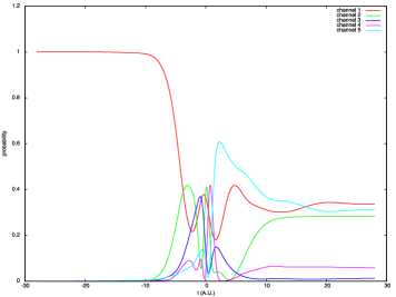
Figure 4: The Si³⁺ + He probabilities as a function of collision time with channel 1 being the initial state for the elastic ($1\rightarrow 1$) and charge exchange transitions ($1\rightarrow 2$ and 5) and excitation ($1\rightarrow 3$ and 4). $n=5$ channel case with $b=1.0$ a₀ and $v_{0}=0.5$.

Figure 5 displays the charge exchange probabilities versus $b$ for $v_{0}=0.5$ a.u. and $n=3$ For the dominant $2\rightarrow 1$ transition, two main probability peaks are evident with the probability falling off to zero by $b=7$ a₀. Additional examples are given in the Supplement.

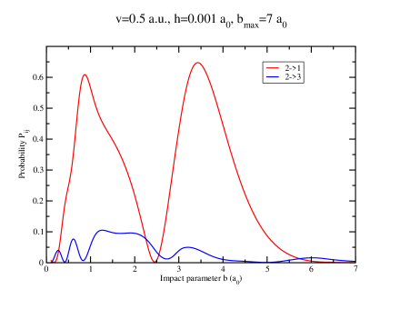
Figure 5: The Si³⁺ + He charge exchange probability for the $2\rightarrow 1$ ($2~{}^{2}\Sigma^{+}\rightarrow 1~{}^{2}\Sigma^{+}$) and $2\rightarrow 3$ ($2~{}^{2}\Sigma^{+}\rightarrow 3~{}^{2}\Sigma^{+}$) transitions versus impact parameter. Three channel case with $v_{0}=0.5$ a.u.

Figure 6 plots the cross section, obtained by integrating the probability distributions from Figure 5, for capture to Si²⁺($3s^{2}~{}^{1}S$) (the 2$\rightarrow$1 transition) which dominates the total charge exchange as the 2$\rightarrow$3 and 2$\rightarrow$4 transitions give small cross sections. The current calculations using the SCMOCC approach are in very good agreement with our earlier QMOCC calculation and a computation performed by Houvault et al. [22]. A similar scattering method was adopted in Ref. [22], but with different diabatic potentials. The ion beam - gas cell measurement of Tawara et al [23] is consistent with all of the calculations, though the uncertainty is rather large. Figure 6 also illustrates a channel convergence study where the integral cross section appears to be approaching convergence by $n=5$, but additional investigations are needed to confirm this result.

There is a second measurement, but of the rate coefficient at 3900 K in an ion trap [24]. A rate coefficient is obtained by averaging the cross section over a Maxwellian velocity distribution. 3900 K corresponds to a center-of-mass kinetic energy of about 0.4 eV and therefore too low of an energy for our SCMOCC method to be valid. However, as Fig. 6 of Ref. [19] shows, the QMOCC results are consistent with the ion trap measurement suggesting that the adopted potentials are reliable. Note also that there is considerable uncertainty in the ion trap temperature.

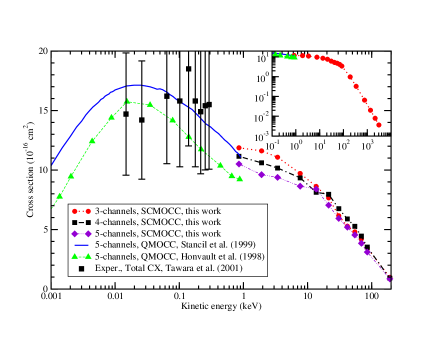
Figure 6: The Si³⁺ + He charge exchange cross section for the $2\rightarrow 1$ transition comparing the current SCMOCC results to earlier QMOCC results. Note the cross section is given as a function of center-of-mass kinetic energy and the results of Ref. [19] used the same diabatic potential as the current work. The experiment is for total charge exchange.

The electron capture cross sections to the Si²⁺($3s3p~{}^{3}P^{o}$) (the 2$\rightarrow$3 transition) are given in the Supplement. The magnitude of the cross sections are about a factor of 20 smaller than for the 2$\rightarrow$1 transition and no experimental data exists. There is reasonable agreement between all calculations, but additional channels are typically required to get small cross sections converged. In summary, the Si³⁺ + He charge exchange system can be an important test case for application to SES devices with $n=3-5$.

2.2 O⁷⁺ + H

Moving to a somewhat larger system, we consider the charge exchange interaction

$${\rm O}^{7+}(1s~{}^{2}S)+{\rm H}(1s~{}^{2}S) \rightarrow {\rm O}^{6+}(1s5\ell~{}^{1}L)+{\rm H}^{+},$$ (15)

$$\rightarrow {\rm O}^{6+}(1s4\ell~{}^{1}L)+{\rm H}^{+},$$ (16)

which was studied with the QMOCC method by Nolte et al. [25]. Here we consider the singlet spin system with nearly degenerate principal quantum number manifolds of 4 and 5 states, giving a total of $n=10$ channels. The singlet adiabatic potential energies are given in Figure 7, while the full diabatic potential matrix is available from Ref. [25].

A series of $n=5$ to $n=10$ channel calculations were performed for $v_{0}=1.0$ a.u. Figure 8 displays the charge exchange probability for the $10\rightarrow 8$ transition whose final state is O⁶⁺($1s5d~{}^{1}D$) + H⁺. A similar plot for elastic scattering is shown in Figure 9 with additional results given in the Supplement.

There is considerable variation in the probabilities with basis size so that this collision system would serve as an interesting test bed for SES devices of moderate size from $n=5-10$. Further, as the size of the system is increased from Na+He to Si³⁺ + He to O⁷⁺ + H, the maximum internal energy difference increases with values of 2.1, 8.8, and 28.5 eV, respectively, allowing for about an order of magnitude in range of energy scale mapping to the SES (see below).

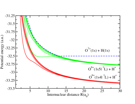
Figure 7: Adiabatic potentials for the OH⁷⁺ singlet system from Nolte et al [25]. The initial channel (10) is given by the blue dashed curve.

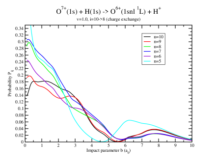
Figure 8: The O⁷⁺ + H probabilities versus impact parameter for the state-resolved charge exchange reaction with product O⁶⁺($1s5d~{}^{1}D$) + H⁺ obtained from SCMOCC calculations with $n=5-10$ channels and $v_{0}=1.0$ a.u.

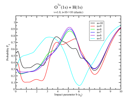
Figure 9: The O⁷⁺ + H probabilities versus impact parameter for elastic scattering obtained from SCMOCC calculations with $n=5-10$ channels and $v_{0}=1.0$ a.u. Note the elastic probability should go to 1.0 as $b\rightarrow\infty$ and is not converged for $b=10$ a₀.

2.3 Low Kinetic Energies: Improvements to the Classical Simulation

The above SCMOCC method assumed a straight line, constant velocity trajectory. This approach is expected to break-down for kinetic energies between 0.1 and 1 keV for the above considered collision systems involving electronic transitions. Or in other words, the straight line SCMOCC method is probably valid for kinetic energies an order of magnitude larger than the maximum internal energy difference

$$K\gtrsim 10|E_{f}-E_{i}|=10|\Delta E|.$$ (17)

To extend the reliability of the SCMOCC method to lower energies, curvilinear trajectories can be adopted by solving for the velocity $dR/dt$ via

$$\frac{dR}{dt}=\pm v_{0}\sqrt{1-\frac{b^{2}}{R^{2}}-\frac{V(R)}{E}}$$ (18)

at each step of the time integration. Here, $v_{0}$ is the initial velocity at infinity, and $E$ is the total energy of the system. However, solving the additional equation (18) increases the computational time, particularly for small values of $v_{0}$. This is related to the requirement of additional time steps in order to stabilize the final probabilities. Figure 10 displays the probability evolution for the Na+He system as a function of collision time comparing the constant velocity case at $v_{0}$=1.0 a.u. to use of equation (18), both for $b=1.0$ a₀. At this high velocity, the probabilities are almost identical as expected, but lowering $v_{0}$ to 0.1 a.u. as shown in Figure 11, results in significant differences. The probabilities versus impact parameter for given in Figure 12.

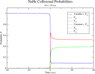
Figure 10: Comparison of Na+He scattering probability evolution with collisions time for constant and variable velocities. Results are presented for $v_{0}=1.0$ a.u., $b=1.0$ a₀, and $n=3$.

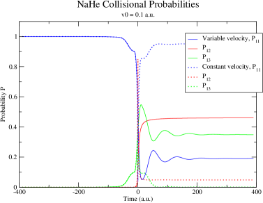
Figure 11: Same as Figure 10 but for $v_{0}=0.1$ a.u.

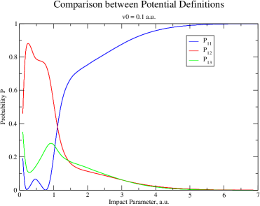
Figure 12: Comparison Na+He scattering probabilities versus impact parameter for a variable velocity with arithmetically-averaged potentials. Results are presented for $v_{0}=0.1$ a.u. and $n=3$.

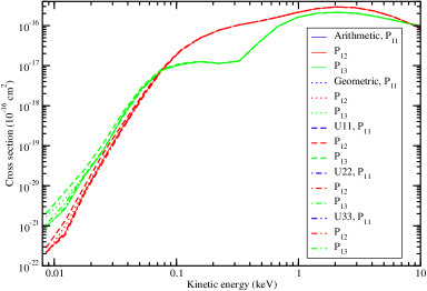
Figure 13: Comparison of the $n=3$ Na+He total cross sections for various potential averaging methods i) arithmetic, ii) geometric, iii) using channel $i=1$, iv) using $i=2$, and v) using $i=5$. Note elastic cross sections are not shown as the various methods give identical results.

While for single channel calculations (i.e., $n=1$) there is no ambiguity in equation (18), for multichannel cases, the $V(R)$ term has presented a theoretical dilemma for many decades. $V(R)$ must be replaced by some superposition, $\bar{V}(R)$, over all channel diagonal diabatic potentials, but the exact prescription is unknown. A number of authors [26, 27, 28, 29] have proposed various schemes including: (i) an arithmetic average, (ii) a geometric average, or (iii) setting $\bar{V}(R)$ equal to the $V_{ii}(R)$ of an individual channel. We find that the probabilities and cross sections computed by any of these schemes are practically indistinguishable down to a kinetic energy of $\sim$0.1 keV. In fact, Delos et al [27] suggested that the exact averaging prescription is unimportant as long as some type of averaging is taken into account, as illustrated in Figures 10-12. For energies less than $\sim$0.1 keV, Figure 13 shows some dispersion of the cross sections for different averaging schemes, but in this energy regime the cross sections become very small. Nevertheless, the arithmetic and geometric approaches give similar results and therefore we default to an arithmetic average of all channels for $\bar{V}(R)$.

2.4 Pushing to Even Lower Kinetic Energies: Ehrenfest Symmetrization

The application of potential averaging is clearly not a robust theoretical procedure and in fact introduces a problem in which the principle of detailed balance,

$$P_{if}(E)=P_{fi}(E),$$ (19)

may be violated [30]. This deficiency becomes worse with decreasing collision energy thereby limiting the applicability of the SCMOCC method. Billing [30] has proposed a correction by introducing a so-called symmetrized Ehrenfest approach. The method, which is not related to Ehrenfest’s Theorems, shifts the relative velocity for a given initial channel and has been shown to give reliable cross sections for a variety of collision systems [30, 31, 32, 33]. We apply it here as a post-processing algorithm which redefines the kinetic energy $K$ of the collision system. For a 2-state case, the kinetic energy is redefined according to

$$E=\bar{K}+\frac{\Delta E}{2}+\frac{\Delta E^{2}}{16\bar{K}},$$ (20)

where $\bar{K}$ is the redefined kinetic energy. It is presumed to be valid for $K\geq\Delta E/4$. So, that for an endoergic process, $E=\Delta E$ with $\Delta E>0$, while $E=0$ and $\Delta E<0$ for exoergic transitions. As an example, Figure 14 compares the integral cross sections for an $n=3$ computation of Si³⁺ + He with and without the symmetrized Ehrenfest approximation for the case of arithmetic-averaged potentials. The former is larger than the uncorrected case for inelastic transitions below 10 keV with the difference increasing with decreasing $K$. In summary, explicitly solving for the relative velocity as a function of time with arithmetic-averaged multichannel potentials and a post-processing shift of the kinetic energy via the symmetrized Ehrenfest approach should allow the SCMOCC method to be applied to compute cross sections for kinetic energies a factor $\sim$100 smaller than with the straight line, constant velocity approximation, that is, approaching kinetic energies as low as 1 eV.

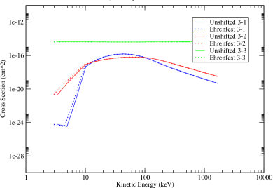
Figure 14: Integral cross sections for Si³⁺ + He with variable velocity illustrating the effect of the symmetrized Ehrenfest approach. As expected, the elastic cross sections are unaffected.

3 Molecular Collisions on an SES Processor

Now we turn to simulating collision problems on a quantum computer using the SES approach.

3.1 Hamiltonian Mapping

To illustrate the SES simulation procedure, we consider the $n=5$ Si³⁺+He charge exchange collision process (14). The collision Hamiltonian $h(t)$ must be rescaled by energy using the method described in Geller et al [16] so that the rescaled Hamiltonian ${\cal H}(t)$ is compatible with the SES processor,

$${\cal H}(t)=\frac{h(t)-c(t)\times I}{\lambda(t)},$$ (21)

where $c(t)$ is the mean of diagonal elements of $h(t)$ and $\lambda(t)$ is the rescaling function such that each matrix element of the SES Hamiltonian ${\cal H}(t)$ lies within the characteristic energy range of the SES device. The simulated (quantum computer) time $t_{qc}$ on the SES processor satisfies a nonlinear relation with respect to the physical time $t$,

$$t_{qc}(t)=\int_{0}^{t}\lambda dt^{\prime}.$$ (22)

The rescaling function $\lambda$ is shown in Figure 15 , and the nonlinear time relationship is shown in Figure 16. As can be seen from Figure 15, near the peak of the rescaling function, the collision energy scale is large where the dynamics becomes significant. With use of the rescaling function, the SES Hamiltonian matrix elements are obtained as shown in Figure 17.

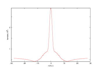
Figure 15: Rescaling factor $\lambda$ as a function of the physical time $t$ for the $n=5$ Si³⁺+He charge exchange collision simulation. Collision parameters are chosen as $b=1.0$ a₀ and $v_{0}=0.5$ a.u.

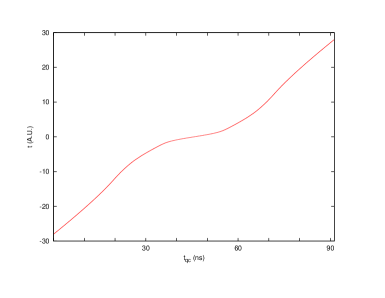
Figure 16: The simulated time $t_{qc}$ as a nonlinear function of the physical time $t$ for the $n=5$ Si³⁺+He charge exchange collision simulation. Collision parameters are chosen as $b=1.0$ a₀ and $v_{0}=0.5$ a.u.

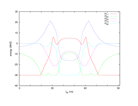
Figure 17: Matrix elements of the SES Hamiltonian $\cal{H}$ as a function of the simulated time $t_{qc}$ for the Si³⁺+He charge exchange collision simulation. Collision parameters are chosen as $b=1.0$ a₀ and $v_{0}=0.5$ a.u.

3.2 Scattering Algorithm and Simulation

Mapping the collision Hamiltonian to the SES Hamiltonian $\cal{H}$ by use of the rescaling function given in Figure 15 and its implementation in a SES processor results in scattering probabilities. Figure 18 depicts the probabilities computed on a classical computer for a simulation of the SES processor for $n=5$. Compared with Figure 4, we see that the dynamics near the time of closest approach are rescaled on the SES processor and occupy most of the simulation. Table 1 shows the final probabilities for transitions out of state 1 on a classical computer and for a simulation of the SES method. These results indicate that the accuracy of the SES method is comparable with that of the classical simulation and the relative error increases with decreasing collision probability. One should note that by mapping the Si³⁺+He collision problem to the SES processor, a single run of the simulation can be completed in about only $70$ ns, independent of $n$.

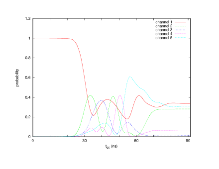
Figure 18: Scattering probabilities versus simulation time on a SES processor for a $n=5$ Si³⁺+He collision with $b=1.0$ a₀ and $v_{0}=0.5$ a.u.

Probability	Classical Simulation	SES simulation	Relative Error
$P_{11}$	$0.3374$	$0.3371$	0.095%
$P_{12}$	$0.2784$	$0.2813$	1.062%
$P_{13}$	$1.2848\times 10^{-2}$	$1.3410\times 10^{-2}$	4.369%
$P_{14}$	$5.8881\times 10^{-2}$	$5.7782\times 10^{-2}$	1.866%
$P_{15}$	$0.3125$	$0.3104$	0.671%

Table 1: Probabilities $P_{if}$ in the $f$-th channel ($i,f=1-5$) for a Si³⁺+He collision in the classical simulator and the SES simulator, respectively. The parameters are chosen as $v_{0}=0.5$ a.u. and $b=1.0$ a₀ with $i=1$ the initial channel.

4 Conclusions

As a potential application for quantum simulation using the single excitation subspace (SES) approach, molecular collisions involving two-atom systems with increasing Hamiltonian dimension are studied using a standard semiclassical molecular-orbital close-coupling (SCMOCC) scattering method. These systems are first studied on a classical computer and then simulations of SES processors are performed. The $n=3$ qubit/molecular channel Na+He excitation problem is extended beyond our earlier work [16] to computations of $n=3-5$ for Si³⁺ + He charge exchange and $n=5-10$ O⁷⁺ + H charge exchange. Good agreement is found between final probabilities and cross sections from the classical and SES simulations based on straight line trajectories above $\sim$1 keV.

To extend the simulations to lower energy, we augment the SCMOCC approach with curvilinear trajectories on various averaged multichannel potentials. Further, to correct for a violation in detailed balance, we explore use of a symmetrized Ehrenfest approach which, combined with potential averaging, will allow for the study of collision systems approaching the chemical regime near 1 eV. As a consequence, the application of the SCMOCC method for quantum simulation with the SES approach appears promising for collision problems with 10 channels or more on similarly sized SES devices.

As outlined in the Introduction, quantum-mechanical calculations on classical computers have currently peaked at the treatment of four- and five-atom systems for time-independent (TI) inelastic and time-dependent reactive scattering, respectively. In the former case, more than 10,000 channels were required, which is a record as far as we are aware for such calculations. A dream today is to be able to perform TI inelastic calculations for the five-atom systems H₂O+H₂ and NO₂+OH which could require $\sim$50,000-500,000 channels on a nine-dimensional potential energy surface. As such calculations can only be envisioned on the next generation of massively parallel CPU/GPU machines, there may be an opportunity for the SES/SCMOCC quantum simulation approach to attack these problems if the construction and operation of large $n$-qubit, fully-connected quantum computers become feasible.

5 Supplement

5.1 Propagator Benchmarking

One of the most interesting applications of the SES method is that of a general-purpose Schrödinger equation solver for TD Hamiltonians [16]. The total time required to perform a single run of the quantum simulation is

$$t_{qu}=t_{qc}+t_{meas},$$ (23)

where $t_{meas}$ is the qubit measurement time which is about $100$ ns. Thus the time for a single run is $\sim 200$ ns independent of the size of the Hamiltonian matrix $n$.

Though the classical runtime depends on a variety of issues, we can still explore the possibility of speedup by benchmarking the time required to classically simulate a TD Hamiltonian. We studied the classical simulation runtime $\tau_{cl}$ for this problem, comparing four standard numerical algorithms: (i) Crank-Nicholson integration [34], (ii) the Chebyshev propagator [35],

$$e^{-(iHt/\hbar)}\approx\sum_{n=0}^{N}a_{n}P_{n}(-iHt/\hbar),$$ (24)

(iii) Runge-Kutta (RK) integration [36] and (iv) time-slicing combined with matrix diagonalization [16]. Both the fourth order Runge-Kutta and the preconditioned adaptive step-size Fehlberg-Runge-Kutta method introduced in Ref. [37] are used in the RK methods here. In the preconditioned approach, a constant preconditioner is applied such that the eigenvalues of the preconditioned Hamiltonian $H_{I}$ are small and thus the RK method converges quickly using the form

$$H_{I}=H-I(E_{\rm max}+E_{\rm min})/2,$$ (25)

where $E_{\rm max}$ and $E_{\rm min}$ are the maximum and minimum eigenvalues of the Hamiltonian $H$, respectively. Here, we use the Gershgorin Circle Theorem [38] to estimate the values of $E_{\rm max}$ and $E_{\rm min}$. For time-slicing combined with diagonalization of a given $H$, the unitary matrix $V$ of its eigenvectors and the diagonal matrix $D$ of its eigenvalues are computed and then $e^{-iHt}$ is obtained by

$$Ve^{-iDt}V^{\dagger}.$$ (26)

Table 2 gives the computation times for each method. The relative errors, compared to the results from a standard high-precision Crank-Nicholson integrator, are bounded by $2\%$. We find that the preconditioned adaptive step-size Fehlberg-Runge-Kutta method is the fastest approach for the specific problem considered here resulting in a speed-up by better than a factor $\sim$220 compared to the standard Crank-Nicholson propagator.

	Crank-Nicholson	Chebyshev	Runge-Kutta	Matrix Diagonalization
without precondition, fixed time step	193.93s (0.001 a.u. per step )	198.35s (0.001 a.u. per step)	137.61s (0.001 a.u. per step)	1.32 s (0.2 a.u. per step)
with precondition, fixed time step	121.24s (0.05 a.u. per step)	N.A.	7.75s (0.1 a.u. per step)	1.31 s (0.2 a.u. per step)
with precondition, adaptive stepsize, exact eigenvalues	N.A.	N.A.	3.80s (Fehlberg-Runge-Kutta local error bound $10^{-4}$)	1.35s (double-step adaptive method with local error bound $10^{-4}$)
with precondition, adaptive stepsize, eigenvalue estimation	N.A.	N.A.	0.88s (local error bound $10^{-4}$)	N.A.

Table 2: Computation time for $n=5$ Si³⁺+He collision problem using various numerical methods. Collision parameters are chosen as $b=1.0$ a₀ and $v_{0}=0.5$ a.u.

5.2 Additional Classical Scattering Results

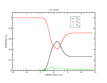
Figure 19: The Si³⁺ + He probabilities as a function of collision time for the elastic ($2\rightarrow 2$) and charge exchange transitions ($2\rightarrow 1$ and $2\rightarrow 3$). $n=3$ channel case with $b=0.6$ a₀, $v_{0}=1.0$ a.u.

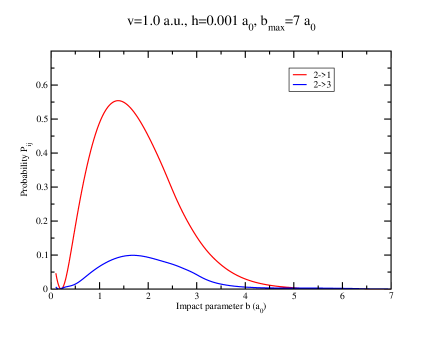
Figure 20: The Si³⁺ + He charge exchange probability for the $2\rightarrow 1$ ($2~{}^{2}\Sigma^{+}\rightarrow 1~{}^{2}\Sigma^{+}$) and $2\rightarrow 3$ ($2~{}^{2}\Sigma^{+}\rightarrow 3~{}^{2}\Sigma^{+}$) transitions versus impact parameter. $n=3$ channel case with $v_{0}=1$ a.u.

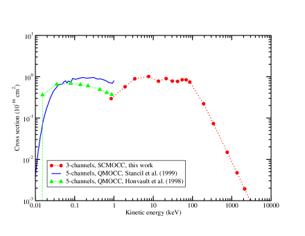
Figure 21: The Si³⁺ + He charge exchange cross section for the $2\rightarrow 3$ transition comparing the current SCMOCC results to earlier QMOCC results. Note the cross section is given as a function of center-of-mass kinetic energy and the results of Ref. [19] used the same diabatic potentials as the current work.

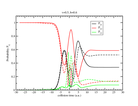
Figure 22: Same as Fig. 3, but comparing $n=3$ channels (solid lines) and $n=4$ channels (dashed lines) for $v_{0}=0.5$ a.u. and $b=0.6$ a₀.

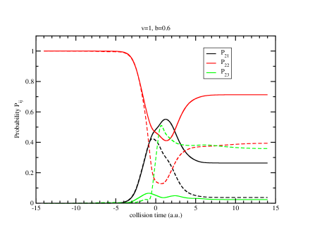
Figure 23: Same as Fig.  22, but for $v_{0}=1.0$ a.u. and $b=0.6$ a₀.

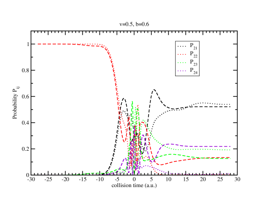
Figure 24: Same as Fig. 22, but comparing $n=4$ channels (dashed lines) and $n=5$ channels (dotted lines) for $v_{0}=0.5$ a.u. and $b=0.6$ a₀.

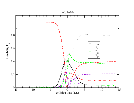
Figure 25: Same as Fig. 22, but comparing $n=4$ channels (dashed lines) and $n=5$ channels (dotted lines) for $v_{0}=1.0$ a.u. and $b=0.6$ a₀.

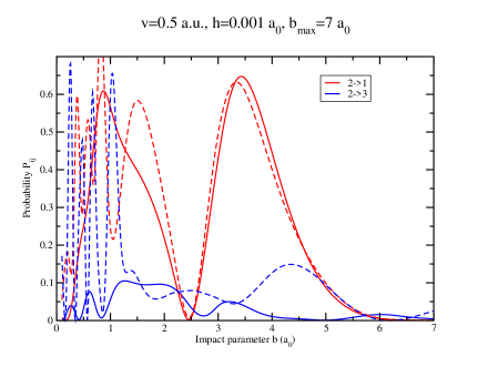
Figure 26: Same as Fig. 5, but comparing $n=3$ channels (solid lines) and $n=5$ channel (dashed lines) for $v_{0}=0.5$ a.u.

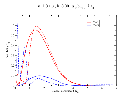
Figure 27: Same as Fig. 26, but comparing $n=3$ channels (solid lines) and $n=4$ channels (dashed lines) for $v_{0}=1.0$ a.u.

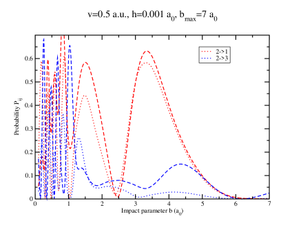
Figure 28: Same as Fig. 26, but comparing $n=4$ channels (dashed lines) and $n=5$ channels (dotted lines) for $v_{0}=0.5$ a.u.

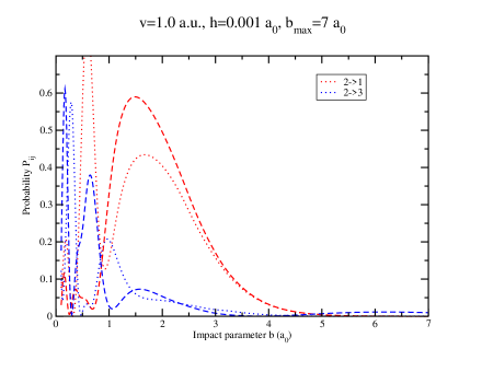
Figure 29: Same as Fig. 26, but comparing $n=4$ channels (dashed lines) and $n=5$ channels (dotted lines) for or $v_{0}=1.0$ a.u.

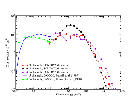
Figure 30: The Si³⁺ + He charge exchange cross section for the $2\rightarrow 3$ transition comparing the current SCMOCC results to earlier QMOCC results. Note the cross section is given as a function of center-of-mass kinetic energy and the results of Ref. [19] used the same diabatic potential as the current work.

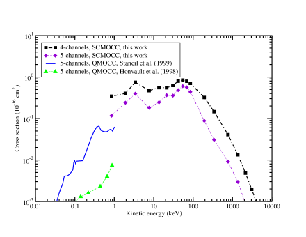
Figure 31: The Si³⁺ + He charge exchange cross section for the $2\rightarrow 4$ transition comparing the current SCMOCC results to earlier QMOCC results. Note the cross section is given as a function of center-of-mass kinetic energy and the results of Ref. [19] used the same diabatic potential as the current work.

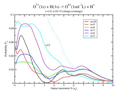
Figure 32: The O⁷⁺ + H probabilities versus impact parameter for the state-resolved charge exchange reaction with product O⁶⁺($1s5p~{}^{1}P$) + H⁺ obtained from SCMOCC calculations with $n=5-10$ channels and $v=1.0$ a.u.

References

- [1] Althorpe S C and Clary D C 2003 Annu. Rev. Phys. Chem. 54 493
- [2] Bowman J M, Czakó G and Fu B N 2011 Phys. Chem. Chem. Phys. 13 8094
- [3] Nyman G and Yu H-G 2013 Int. Rev. Phys. Chem. 32 39
- [4] Wang D 2006 J. Chem. Phys. 124 201105
- [5] Yang B H, Zhang P, Wang X, Stancil P C, Bowman J M, Balakrishnan N and Forrey R C 2015 Nature Comm. 6 6629
- [6] Olivares-Amaya R, Watson M A, Edgar R G, Vogt L, Shao Y and Aspuru-Guzik A 2010 J. Chem. Theory and Comput. 6 135
- [7] Werner H J, Knowles P J, Manby F R, Schütz M, et al MOLPRO 2010 http://www.molpro.net
- [8] Braams B J and Bowman J M 2009 Int. Rev. Phys. Chem. 28 577
- [9] Aspuru-Guzik A, Dutoi A D, Love P J and Head-Gordon M 2005 Science 309 1704
- [10] Lanyon B P, Whitfield J D, Gillett G G, Goggin M E, Almeida M P, Kassal I, Biamonte J D, Mohseni M, Powell B J, Barbieri M, Aspuru-Guzik A, and White A G 2010 Nature Chem. 2 106
- [11] Lu D, Xu N, Xu R, Chen H, Gong J, Peng X and Du J 2011 Phys. Rev. Lett. 107 020501
- [12] Lidar D A and Wang H 1999 Phys. Rev. E 59 2429
- [13] Smirnov A Yu, Savel’eV S, Mourokh L G and Nori F 2007 Euro. Phys. Lett. 80 67008
- [14] Kassal I, Jordan S P, Love P J, Mohseni M and Aspuru-Guzik A 2008 Proc. Nat. Acad. Sci. USA 105 18681
- [15] Pritchett E J, Benjamin C, Galiautdinov A, Geller M R, Sornborger A T, Stancil P C and Martinis J M 2010 arXiv:1008.0701
- [16] Geller M R, Martinis J M, Sornborger A T, Stancil P C, Pritchett E J, You H and Galiautdinov A 2015 Phys. Rev. A 91 062309
- [17] Child M S 1984 Molecular CollisionTheory, Academic Press
- [18] Lin C Y, Stancil P C, Liebermann H-P, Funke P and Buenker R J 2008 Phys. Rev. A 78 052706
- [19] Stancil P C, Clarke N J, Zygelman B and Cooper D L 1999 J. Phys. B 32 1523
- [20] Kimura M and Lane N F 1990 Adv. At. Mol. Phys. 26 79
- [21] Zygelman B, Cooper D L, Ford M J, Dalgarno A, Gerratt J and Raimondi M 1992 Phys. Rev. A 46 3846
- [22] Honvault, P., Bacchus-Montabonel, M. C., Gargaud, M., & McCarroll, R. 1998, Chem. Phys., 238, 401
- [23] Tawara, H., Okuno, K., Fehrenbach, C. W., Verzani, C., Stockli, M. P., Depaola, B. D., Richard, P., & Stancil, P. C. 2001, Phys. Rev. A, 63, 062701
- [24] Fang, Z. & Kwong, V. H. S. 1997, Astrophys. J., 483, 527
- [25] Nolte L, Wu Y, Stancil P C, Liebermann H-P, Buenker R J, Schultz D R, Hui Y, Draganić I N, Havener C C and Raković M J 2016 to be submitted
- [26] Bates D R and Crothers D S 1970 Proc. R. Soc. A 315 465
- [27] Delos J B, Thorson W R and Knudson S K 1972 Phys. Rev. A 6 709
- [28] Riley M E 1973 Phys. Rev. A 8 742
- [29] Liang J R and Freed K F 1975 Phys. Rev. Lett. 34 849
- [30] Billing G D 2003 The Quantum Classical Theory, Oxford Univ. Press
- [31] Semenov A, Ivanov M and Babikov D 2013 J. Chem. Phys. 139 074306
- [32] Ivanov M, Dubernet M-L and Babikov D 2014 J. Chem. Phys. 140 134301
- [33] Babikov D and Semenov A 2016 J. Phys. Chem. in press
- [34] Thomas J W 1995 Numerical Partial Differential Equations: Finite Difference Methods. Texts in Applied Mathematics 22. Berlin, New York: Springer-Verlag
- [35] Leforestier C, Bisseling R H, Cerjan C, Feit M D, Friesner R, Guldberg A, Hammerich A, Jolicard G, Karrlein W, Meyer H-D, Lipkin N, Roncero O and Kosloff R 1991 J. Computational Phys. 94 59
- [36] Press W H, Teukolsky S A, Vetterling W T and Flannery B P 2007 Numerical Recipes, 3rd Edition, Cambridge University Press
- [37] Tremblayand J C and Carrington T Jr. 2004 J. Chem. Phys. 121 11535
- [38] Golub G H and Van Loan C F 1996 Matrix Computations. Baltimore: Johns Hopkins University Press, p. 320