Numerical RHD simulations
of flaring chromosphere with Flarix

Abstract

Flarix is a radiation–hydrodynamical (RHD) code for modeling of the response of the chromosphere to a beam bombardment during solar flares. It solves the set of hydrodynamic conservation equations coupled with NLTE equations of radiative transfer. The simulations are driven by high energy electron beams. We present results of the Flarix simulations of a flaring loop relevant to the problem of continuum radiation during flares. In particular we focus on properties of the hydrogen Balmer continuum which was recently detected by IRIS.

1 Introduction

Recent advances in numerical RHD (radiation hydrodynamics) allow to solve complex problems of time evolution of the solar atmosphere affected by various flare processes ([Allred et al. (2005), Allred et al. 2005], [Kašparová et al. (2009), Kašparová et al. 2009], [Varady et al. (2010), Varady et al. 2010], [Allred et al. (2015), Allred et al. 2015]). Resulting time-dependent atmospheric models (i.e. variations of the temperature, density, ionization and excitation of various species etc.) are then used as an input for synthesis of spectral lines and continua of atoms and ions under study. One of the ’hot topics’ which attracts a substantial attention is the behavior of the so-called white light flares, and namely the problem of continuum formation. Recent finding of [Heinzel & Kleint (2014)] that the hydrogen Balmer continuum, previously rarely detected around the Balmer jump, can be easily seen in the flare spectra taken by Interface Region Imaging Spectrograph IRIS ([De Pontieu et al. (2014), De Pontieu et al. 2014]) in the NUV channel represents a strong motivation for new numerical simulations. In this paper we first briefly describe the RHD technique on which our code Flarix is based and then use the flare simulations to predict the time behavior of the Balmer continuum. We then discuss the importance of the Balmer continuum for energy balance in the flaring chromosphere.

2 RHD code Flarix

The hybrid radiation–hydrodynamical code Flarix is based on three originally autonomous, now within Flarix fully integrated, codes: a test-particle (TP) code, a one-dimensional hydrodynamical (HD) code and time dependent NLTE radiative transfer code (for a detailed description of the code see [Kašparová et al. (2009)] and [Varady et al. (2010)]) . Flarix is able to model several processes, which according to contemporary and generally accepted flare models occur concurrently in flares and play there important roles. The transport, scattering and progressive thermalization of the beam electrons due to Coulomb collisions with particles of ambient plasma in the magnetized flaring atmosphere and the resulting flare heating corresponding to the local energy losses of beam electrons is calculated using an approach proposed by [Bai (1982)] and [Karlický & Hénoux (1992)] based on test particles and Monte Carlo method. This approach, fully equivalent to direct solution of the corresponding Fokker-Planck equation ([MacKinnon & Craig (1991), MacKinnon & Craig 1991]), provides a flexible way to model many various aspects of the beam electron interactions with the ambient plasma, converging magnetic field in the flare loop or with additional electric fields ([Varady et al. (2014), Varady et al. 2014]). These were proposed in various modifications of the standard CSHKP flare model (e.g. [Turkmani et al. (2006), Turkmani et al. 2006], [Brown et al. (2009), Brown et al. 2009], [Gordovskyy & Browning (2012), Gordovskyy & Browning 2012]) or they can be related to the return current propagation ([van den Oord (1990), van den Oord 1990)]). Owing to TP approach, the detailed distribution function of beam electrons is known at any instant and position along the flare loop. This information can be used to calculate a realistic distribution of HXR bremsstrahlung sources within the loop, their position size, spectra and directivity of emanating HXR emission ([Moravec et al. (2013), Moravec et al. 2013], [Moravec et al. (2016), Moravec et al. 2016]).

Starting point of Flarix simulations are parameters of the non-thermal beam electrons. They are assumed to obey a single power law in energy, so their initial spectrum (in units of electrons cm^-2 s^-1 keV^-1) is

$$F(E,t)=\left\{\begin{array}[]{ll}g(t)F(E)=g(t)\ (\delta-2)\frac{F_{\mathrm{max}}}{E_{0}^{2}}\left(\frac{E}{E_{0}}\right)^{-\delta}&,\ \ \ \mbox{for}\ \ \ E_{0}\leq E\leq E_{1}\\ 0&,\ \ \ \mbox{for other}\ E\ .\\ \end{array}\right.\ \$$ (3)

The time dependent electron flux at the loop-top is determined by $g(t)\in\langle 0,1\rangle$, a function describing the time modulation of the beam flux, the maximum energy flux $F_{\mathrm{max}}$ , i.e. the energy flux of electrons with $E\geq E_{0}$ at $g(t)=1$, the low and high-energy cutoffs $E_{0}$, $E_{1}$, respectively, and the power-law index $\delta$. These parameters can be derived either from observations like RHESSI ([Lin et al. (2002), Lin et al. 2002]) or set up arbitrarily. Another important parameter is the initial pitch angle distribution of non-thermal electrons $\Theta=\Theta(\vartheta_{0})$. In case the function $\Theta(\vartheta_{0})$ is normalized, the angle dependent initial electron flux is

$$F(E,\vartheta_{0},t)=\Theta(\vartheta_{0})F(E,t)\ .$$ (4)

The initial pitch angle distribution can be chosen by the user.

The 1D one fluid HD part of Flarix calculates the state and evolution of the plasma along semicircular magnetic field lines. The following set of equations is solved

$$\frac{\partial\rho}{\partial t}+\frac{\partial}{\partial s}(\rho u)=0\qquad\frac{\partial\rho u}{\partial t}+\frac{\partial}{\partial s}(\rho u^{2})=-\frac{\partial P}{\partial s}+F_{\mathrm{g}}$$

$$\frac{\partial E}{\partial t}+\frac{\partial}{\partial s}(uE)=-\frac{\partial}{\partial s}(uP)-\frac{\partial}{\partial s}{\mathcal{F}}_{\mathrm{c}}+\mathcal{S}\$$ (5)

where $s$ and $u$ are the position and velocity of plasma along the fieldlines, respectively, and $\rho$ is the plasma density. The gas pressure $P$, total plasma energy $E$, and the source term ${\mathcal{S}}$ are

$$P=n_{\mathrm{H}}(1+x+\varepsilon)k_{\mathrm{B}}T\,,\qquad E=\frac{P}{\gamma-1}+\frac{1}{2}\rho u^{2}\ ,\qquad{\cal S}={\cal H}-{\cal R}+{\cal Q}\,,$$ (6)

where $\gamma=5/3$ is the ratio of specific heats, $k_{\mathrm{B}}$ the Boltzmann constant, and $T$ the temperature. The time-dependent hydrogen ionization $x$ is provided by the NLTE code, $\varepsilon$ accounts for the contribution from metals.

The terms on the right hand side of the system are: $F_{\mathrm{g}}$ the component of the gravity force in the parallel direction to the fieldlines, ${\mathcal{F}}_{\mathrm{c}}$ the heat flux calculated according to the Spitzer classical formula, and ${\mathcal{S}}$ includes all kinds of heating, i.e. mainly the total flare heating ${\cal H}$, the quiescent heating ${\cal Q}$ assuring stability of the initial unperturbed atmosphere, and ${\mathcal{R}}$ the radiative losses. The latter are computed in the NLTE part of the code by solving the time-dependent radiative-transfer problem in the bottom part of the flaring loop, for all relevant transitions of hydrogen, CaII and MgII (addition of helium losses is now in progress). In optically-thin regions of the transition region and corona the loss function of [Rosner et al. (1978), Rosner et al. (1978)] is used.

Using the instant values of $T$, $n_{\mathrm{H}}$, and beam electron energy deposit obtained by the HD and TP codes, time-dependent NLTE radiative transfer for hydrogen is solved in the lower parts of the loop in a 1D plan-parallel approximation. The hydrogen atom is approximated by a five level plus continuum atomic model. The level populations $n_{i}$ are determined by the solution of the time-dependent system of equations of statistical equilibrium and charge and particle conservation equations

$$\frac{{\rm d}n_{i}}{{\rm d}t}=\sum\limits_{j\neq i}n_{j}P_{ji}-n_{i}\sum\limits_{j\neq i}P_{ij}\ \qquad n_{\mathrm{e}}=n_{\mathrm{p}}+\varepsilon n_{\mathrm{H}}\,\qquad\sum_{j=1}^{5}n_{j}+n_{\mathrm{p}}=n_{\mathrm{H}},$$ (7)

where $n_{\mathrm{e}}$ and $n_{\mathrm{p}}$ are the electron and proton densities, respectively. $P_{ij}$ contain sums of thermal and non-thermal collisional rates and radiative rates, the latter being preconditioned in the frame of MALI method ([Rybicki & Hummer (1991), Rybicki & Hummer 1991]). The NLTE part of Flarix gives a consistent solution for the non-equilibrium (time-dependent) hydrogen ionization.

3 Simulation of a short-duration electron beam heating

Here we present results of a simulation of the electron beam heating with a trapezoidal time modulation (see Fig. 1), $\delta=3$, $E_{0}=20$ keV, $E_{1}=150$ keV, and $F_{\mathrm{max}}=4.5\times 10^{10}$ erg cm^-2 s^-1 which represents a short beam-pulse heating with a moderate electron beam flux. As the initial unperturbed atmosphere we used the hydrostatic VAL-C atmospheric model of [Vernazza et al. (1981)] with a hydrostatic extension into the transition region and corona. Response of this atmosphere to the heating and the temporal evolution of the Balmer line emission is discussed in detail in [Kašparová et al. (2009)], see model H_TP_D3 there. In this particular RHD simulation, a simplified approach of [Peres et al. (1982)] was used to compute chromospheric radiative losses ${\mathcal{R}}$.

Figure 1: Time modulation $g(t)$ of the beam flux (solid line), dotted line denotes $\int_{0}^{t}g(t^{\prime})\,\mathrm{d}t^{\prime}=E_{\mathrm{tot}}(t)/F_{\mathrm{max}}$. Total energy deposit is $E_{\mathrm{tot}}=F_{\mathrm{max}}\int_{0}^{t_{1}}g(t)\,\mathrm{d}t\$, where $t_{1}$ is the duration of the energy deposit. See also Eqs. (3).

4 Hydrogen Balmer continuum

The time evolution of hydrogen atomic level populations, proton and electron densities and plasma temperatures has been used to synthesize the hydrogen Balmer continuum. For this purpose we have performed the formal solution of the transfer equation and obtained the time evolution of the Balmer continuum intensities. The results of Flarix simulations are shown in Fig. 2. The time evolution of temperature, primarily due to the electron beam heating, is shown in the top left panel. The time evolution of electron density consisting of the non-equilibrium contribution from hydrogen plus contribution from metals dominating around the temperature minimum region is shown in the top right panel. Around the height of 1000 km the electron density is substantially enhanced (reaching 10¹³ cm^-3) which is typical for stronger flares. The bottom panel shows time evolution of the Balmer-continuum spectrum. The vertical dashed line is drawn at the wavelength 2830 Å  which corresponds to the NUV spectral window of IRIS used by [Heinzel & Kleint (2014)] to detect the Balmer continuum. The light curve at this particular wavelength is then shown in Fig. 3.

  

  

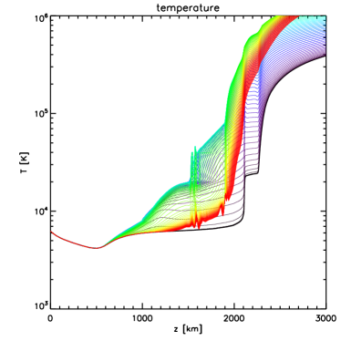
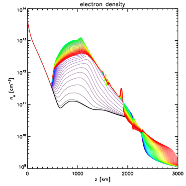
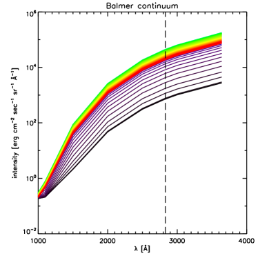
Figure 2: Results of Flarix simulations for the trapezoidal electron beam pulse described in Section 3. The three panels show, respectively, the time evolution of temperature (top left), electron density (top right), and the hydrogen Balmer-continuum spectrum (bottom). In the latter panel we indicate the wavelength used by IRIS to detect this continuum (see the vertical dashed line). The gray-scale coding represents the time evolution from initial stages (black) through the flare maximum (light gray) up to the end of simulation (dark gray). In the online version of the paper the time evolution is color coded – for increasing time the colors change from black to blue-green-yellow-red.

Figure 3: Simulated time evolution (light-curve) of the hydrogen Balmer continuum intensity at the wavelength selected for IRIS detection in the NUV channel (dashed vertical line in Fig. 2).

5 Discusion and conclusions

Our first Flarix simulations of time evolution of the hydrogen Balmer-continuum emission are qualitatively consistent with the IRIS NUV light curves obtained by [Heinzel & Kleint (2014)] and [Kleint et al. (2016)]. They show impulsive intensity rise followed by a gradual decrease. Rather slow non-equilibrium hydrogen recombination is perceptible in the light curve as expected but a more detailed analysis of this behavior is needed. However, for the present short trapezoidal electron-beam pulse lasting only a few seconds (Fig. 1), the synthetic intensity is lower in comparison with observations from [Heinzel & Kleint (2014)] or [Kleint et al. (2016)]. This can be due to several reasons. First, the electron-beam flux used in this particular simulation is almost an order of magnitude lower than that derived from RHESSI spectra in [Kleint et al. (2016)]. Second, the Balmer-continuum intensity was found to be increasing with the boundary pressure at $T$=10⁵ K (see Table 1 in [Kleint et al. (2016)]) and the pressure in this simulation is low due to insufficient evaporation. The beam duration is short and we may expect that a long-duration pulse or series of beam pulses will lead to stronger Balmer continuum, more consistent with the IRIS observations. Finally, for stronger beams one should not neglect the return currents which will modify the non-thermal hydrogen excitation and ionization ([Karlický et al. (1992), Karlický et al. 2004]). Study of all these aspects is now in progress. We have also found that the chromospheric radiative cooling at the pulse maximum is dominated by the hydrogen subordinate continua and namely by the Balmer continuum – for static flare models this was already demonstrated by [Avrett et al. (1986)]. Therefore, this continuum plays a critical role in the energy balance of the flaring chromosphere, the site where most of the electron-beam energy is deposited. Since the Balmer continuum is mostly optically thin in the flaring chromosphere, the total radiative losses integrated along the relevant formation heights are directly related to the observed Balmer-continuum spectral intensity. The IRIS observations thus provide an extremely important constraint on the flare energetics. Moreover, accepting the idea of backwarming of the flare photosphere, one gets directly the amount of radiative energy which should heat the lower atmospheric layers. This issue is discussed in [Kleint et al. (2016)] using the IRIS and optical/infrared continuum observations. We conclude that the Flarix simulations coupled to broad-band continuum observations should provide a clue to the long-lasting mystery of the white-light flares.

This project was supported by the EC Program FP7/2007-2013 under the F-CHROMA agreement No. 606862 and by the grant P209/12/0103 of the Czech Funding Agency (GACR).

References

- [Allred et al. (2015)] Allred, J.C., Kowalski, A.F., Abbett, & Carlsson, M. 2015, ApJ, 809, 104
- [Allred et al. (2005)] Allred, J.C., Hawley, S.L., Abbett, W.P., & Carlsson, M. 2005, ApJ, 630, 573
- [Avrett et al. (1986)] Avrett, E.H., Machado, M.E., & Kurucz, R.L. 1986, in The lower atmosphere of solar flares, ed. D.F. Neidig, Sunspot (NSO), New Mexico, 216
- [Bai (1982)] Bai, T. 1982, ApJ, 259, 341
- [Brown et al. (2009)] Brown, J.C., Turkmani, R., Kontar, E.P., MacKinnon, A.L., & Vlahos, L. 2009, A&A, 508, 993
- [De Pontieu et al. (2014)] De Pontieu, B., Title, A.M., Lemen, J.R., et al. 2014, Sol. Phys., 289, 2733
- [Gordovskyy & Browning (2012)] Gordovskyy, M. & Browning, P.K. 2012, Sol. Phys., 277, 299
- [Heinzel & Kleint (2014)] Heinzel, P. & Kleint, L. 2014, ApJ, 794:L23
- [Karlický & Hénoux (1992)] Karlický, M. & Hénoux, J.C. 1992, A&A, 264, 679
- [Karlický et al. (1992)] Karlický, M., Kašparová), J., & Heinzel, P. 2004, A&A, 416, L13
- [Kašparová et al. (2009)] Kašparová, J., Varady, M., Heinzel, P., Karlický, M., & Moravec, Z. 2009, A&A, 499, 923
- [Kleint et al. (2016)] Kleint, L., Heinzel, P., Judge, P., & Krucker, S. 2016, ApJ, in press (arXiv:1511.04161v1)
- [Lin et al. (2002)] Lin, R.P., Dennis, B.R., Hurford, G.J., et al. 2002, Sol. Phys., 210, 3
- [MacKinnon & Craig (1991)] MacKinnon, A.L. & Craig, I.J.D. 1991, A&A, 251, 693
- [Moravec et al. (2013)] Moravec, Z., Varady, M., Karlický, M., & Kašparová, J. 2013, Central European Astrophys. Bull., 37, 535
- [Moravec et al. (2016)] Moravec, Z., Varady, M., Kašparová, J., & Kramoliš, D., 2016, AN, in press
- [van den Oord (1990)] van den Oord, G.H.J. 1990, A&A, 234, 496
- [Peres et al. (1982)] Peres, G., Serio, S., Vaiana, G.S., & Rosner, R. 1982, ApJ, 252, 791
- [Rybicki & Hummer (1991)] Rybicki, G.B. & Hummer, D.G. 1991, ApJ, 245, 171
- [Rosner et al. (1978)] Rosner, R., Tucker, W.H., & Vaiana, G.S. 1978, ApJ, 220, 643
- [Turkmani et al. (2006)] Turkmani, R., Cargill, P.J., Galsgaard, K., Vlahos, L., & Isliker, H. 2006, A&A, 449, 749
- [Varady et al. (2010)] Varady, M., Kašparová, J., Moravec, Z., Heinzel, P., & Karlický, M. 2010, in IEEE Transactions on Plasma Science, 38, 2249
- [Varady et al. (2014)] Varady, M., Karlický, M., Moravec, Z., & Kašparová, J. 2014, A&A, 563, A51
- [Vernazza et al. (1981)] Vernazza, J.E., Avrett, E.H., & Loeser, R. 1981, ApJS, 45, 635