New calibrations for abundance determinations in H ii regions

Abstract

Simple relations for deriving the oxygen abundance in H ii regions with intensities of the three strong emission lines $R_{2}$, $R_{3}$, and $N_{2}$ ($R$ calibration) or $S_{2}$, $R_{3}$, and $N_{2}$ ($S$ calibration) in their spectra are suggested. A sample of 313 reference H ii regions of the counterpart method ($C$ method) is used as calibrating data points. Relations for the determination of nitrogen abundances, the $R$ calibration, are also constructed. We find that the oxygen and nitrogen abundances in high-metallicity H ii regions can be estimated using the intensities of the two strong lines $R_{2}$ and $N_{2}$ (or $S_{2}$ and $N_{2}$ for oxygen) only. The corresponding two-dimensional relations are provided. There are considerable advantages of the suggested calibration relations as compared to the existing ones. First, the oxygen and nitrogen abundances estimated through the suggested calibrations agree with the $T_{e}$-based abundances within $\sim 0.1$ dex over the whole metallicity range, i.e., the relative accuracy of the calibration-based abundances is 0.1 dex. Although we constructed distinct relations for high- and low-metallicity objects, the separation between these two can be simply obtained from the intensity of the $N_{2}$ line. Moreover, the applicability ranges of the high- and low-metallicity relations overlap for adjacent metallicities, i.e., the transition zone disappears. Second, the oxygen abundances produced by the two suggested calibrations are in remarkable agreement with each other. In fact, the $R$-based and $S$-based oxygen abundances agree within $\sim$0.05 dex in the majority of cases for more than three thousand H ii region spectra.

1 Introduction

Reliable chemical abundance determinations are essential for a wide variety of investigations of galaxies and their evolution. For example, on global scales they are one of the key parameters in the study of the luminosity-metallicity and mass-metallicity relations of galaxies, their evolution with time, and their dependence on environment or star formation rate (e.g., Lequeux et al., 1979; Grebel et al., 2003; Tremonti et al., 2004; Erb et al., 2006; Panter et al., 2008; Zahid et al., 2012; Sánchez et al., 2013; Peng & Maiolino, 2014; Zahid et al., 2014; Izotov et al., 2015, to just name a few of the many studies). Local measurements within galaxies reveal the position-dependent metallicity of the chosen tracer population and may show abundance gradients, which in turn hold clues about galaxy evolution (e.g., Searle, 1971; Janes, 1979; Maciel & Quireza, 1999; Harbeck et al., 2001; Andrievsky et al., 2002; Chen et al., 2003; Mehlert et al., 2003; Cioni, 2009; Haschke et al., 2012; Boeche et al., 2013, 2014; Pilyugin et al., 2014, 2015).

The metallicity of star-forming galaxies at the present epoch can be estimated from the emission-line spectra of H ii regions, which are easily obtained even over greater distances. It is believed that the direct $T_{e}$ method (e.g., Dinerstein, 1990) provides the most reliable abundance determinations in H ii regions. Abundance determinations through the direct $T_{e}$ method require high-precision spectroscopy of H ii regions in order to detect the weak auroral lines such as [O iii]$\lambda$4363 or/and [N ii]$\lambda$5755. Unfortunately, these auroral lines are often rather faint and thus may be detected only in the spectra of a limited number of H ii regions. The abundances in other H ii regions are then usually estimated through the method suggested by Pagel et al. (1979) and Alloin et al. (1979). The idea of this method (traditionally called the strong-line method) is to establish the relation between the (oxygen) abundance in an H ii region and some combination of the intensities of strong emission lines in its spectrum, i.e., the combination of the intensities of these strong lines is calibrated in terms of the metallicity of the H ii region. Therefore, such a relation is usually called a “calibration” and serves to convert metallicity-sensitive emission-line combinations into metallicity estimations.

Numerous calibrations based on the emission lines of different elements were suggested (Edmunds & Pagel, 1984; Dopita & Evans, 1986; McGaugh, 1991; Zaritsky, Kennicutt & Huchra, 1994; Pilyugin, 2000, 2001a; Kewley & Dopita, 2002; Pettini & Pagel, 2004; Tremonti et al., 2004; Pilyugin & Thuan, 2005; Stasínska, 2006; Pilyugin et al., 2010; Marino et al., 2013; Morales-Luis et al., 2014, among many others). A prominent characteristic of all the calibrations is that there is no unique relation that is applicable across the whole range of metallicities of H ii regions. Instead, a calibration relation for a limited range of metallicities or distinct calibration relations for different intervals of metallicities (usually at high or at low metallicities) are constructed. One has to know a priori to which interval of metallicity the H ii region belongs in order to choose the relevant calibration relation (e.g., Kewley & Dopita, 2002; Blanc et al., 2015). This can result in a wrong choice of the calibration relation and, as a consequence, in large uncertainties in the abundances of the H ii regions. This problem is particularly difficult for H ii regions that lie near the boundary of the applicability of the calibration relation.

The most important characteristic of the calibration is a sample of calibrating data points to be used in the construction of the calibration relation. Grids of photoionization models of H ii regions can be used to establish a relation between strong-line intensities and oxygen abundances (e.g., McCall, Rybski & Shields, 1985; Dopita & Evans, 1986; McGaugh, 1991; Kewley & Dopita, 2002; Dopita et al., 2013). Such calibrations are usually referred to as theoretical or model calibrations. On the other hand, a sample of H ii regions in which the oxygen abundances are determined through the direct $T_{e}$ method can serve as basis of a calibration (e.g., Pilyugin, 2000, 2001a; Pilyugin et al., 2010; Marino et al., 2013). Such calibrations are usually called empirical calibrations. There are also a hybrid calibrations where both the H ii regions with directly measured abundances and the photoionization models of H ii regions are used (e.g., Pettini & Pagel, 2004).

There are large systematic discrepancies between the abundance values produced by different published calibrations. The theoretical (or model) calibrations generally produce oxygen abundances that are by factors of 1.5 to 5 higher than those derived through the direct $T_{e}$ method or through empirical calibrations (e.g., Kennicutt, Bresolin & Garnett, 2003; Pilyugin, 2003; Kewley & Ellison, 2008; Bresolin et al., 2009; Moustakas et al., 2010; López-Sánchez & Esteban, 2010; López-Sánchez et al., 2012). Thus, at the present time there is no absolute scale for metallicities of H ii regions. The empirical calibrations have advantages as compared to the theoretical calibrations. The empirical metallicity scale is well defined in terms of the abundances in H ii regions derived through the direct $T_{e}$ method, i.e., in that sense the empirical metallicity scale is absolute. The abundances in H ii regions obtained through the different empirical calibrations are compatible with each other as well as with the direct $T_{e}$-based abundances. The empirical metallicity scale is likely the preferable metallicity scale at present.

The construction of an empirical calibration encounters the following difficulty. Not all direct abundances are of high precision since the measurements of the weak auroral lines can involve considerable errors. Therefore the choice of a sample of H ii regions with reliable abundances is not a trivial task. We recently suggested a new method (the “C method”) for abundance determinations in H ii regions, which can be used over the whole range of metallicities of H ii regions and which provides oxygen and nitrogen abundances on the same metallicity scale as the classical $T_{e}$ method (Pilyugin et al., 2012). It is important that the $C$ method allows one to choose a sample of H ii regions with reliable $T_{e}$-based abundances (Pilyugin et al., 2012, 2013; Zinchenko et al., 2016).

The goal of the present study is to establish simple calibration relations that provide the oxygen and nitrogen abundance determinations over the whole range of H ii region metallicities with relative errors less than 0.1 dex. The paper is structured as follows. The sample of calibrating data points is reported in Section 2. The calibration relations are constructed in Section 3. The discussion is given in Section 4, followed by a summary (Section 5).

Throughout the paper, we will use the following standard notations for the line intensities:
$R_{2}$ = $I_{\rm[O\,II]\lambda 3727+\lambda 3729}/I_{{\rm H}\beta}$,
$N_{2}$ = $I_{\rm[N\,II]\lambda 6548+\lambda 6584}/I_{{\rm H}\beta}$,
$S_{2}$ = $I_{\rm[S\,II]\lambda 6717+\lambda 6731}/I_{{\rm H}\beta}$,
$R_{3}$ = $I_{{\rm[O\,III]}\lambda 4959+\lambda 5007}/I_{{\rm H}\beta}$.

Based on these definitions, the excitation parameter $P$ is expressed as $P$ = $R_{3}$/$R_{23}$ = $R_{3}$/($R_{2}$ + $R_{3}$). The electron temperatures will be given in units of 10⁴K. The notation (O/H)^∗ = 12 +log(O/H) will be used in order to permit us to write our equations in a compact way.

2 The sample of the calibrating data points

Figure 1: The normalized histograms of the oxygen and nitrogen abundances for our sample of calibrating H ii regions.

It was noted above that the choice of a sample of H ii regions with reliable abundance determinations is not a trivial task. Such a sample was compiled in the framework of the $C$ method for abundance determinations in H ii regions (Pilyugin et al., 2012). This selection of reference H ii regions is based on the idea that if an H ii region belongs to the sequence of photoionized nebulae, and its line intensities are measured accurately, then different methods based on different emission lines should yield similar physical characteristics (such as electron temperatures and abundances) for a given object (Thuan et al., 2010; Pilyugin et al., 2012).

The original compilation of reference H ii region spectra with detected auroral lines (and, consequently, with $T_{e}$-based abundances) that was created in Pilyugin et al. (2012) has been updated by adding more recent measurements of H ii regions. The latest version of the collection includes 965 $T_{e}$-based abundances. Using those data we select a sample of reference H ii regions for which all absolute differences in their oxygen abundances (O/H)${}_{C_{\rm ON}}$ – (O/H)${}_{T_{e}}$ and (O/H)${}_{C_{\rm NS}}$ – (O/H)${}_{T_{e}}$ and nitrogen abundances (N/H)${}_{C_{\rm ON}}$ – (N/H)${}_{T_{e}}$ and (N/H)${}_{C_{\rm NS}}$ – (N/H)${}_{T_{e}}$ are less than 0.1 dex. This sample of reference H ii regions contains 313 objects (Zinchenko et al., 2016) and will be used as calibrating data set in the present study. Hence, here we use the empirical metallicity scale defined by H ii regions with abundances derived through the direct method ($T_{e}$ method).

Fig. 1 shows the normalized histograms of the oxygen and nitrogen abundances for the H ii regions of our reference sample.

3 Calibration relations

3.1 Approach

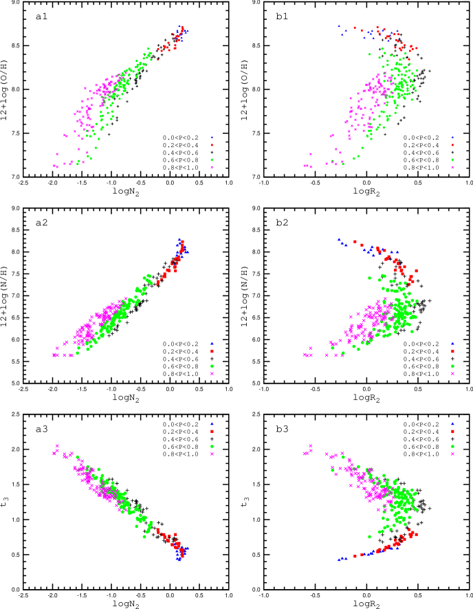
Figure 2: Oxygen abundances (panel $a1$), nitrogen abundances (panel $a2$), and electron temperatures $t_{3}$ (panel $a3$) as a function of the nitrogen line $N_{2}$ intensity for our sample of H ii regions used as calibrating data points. H ii regions with different values of the excitation parameter $P$ are plotted with different symbols as explained in the legend. The panels $b1,b2,b3$ show the same as the panels $a1,a2,a3$ but as a function of the oxygen line $R_{2}$ intensity.

The panels in the left column of Fig. 2 show the oxygen abundances (panel $a1$), nitrogen abundances (panel $a2$), and electron temperatures $t_{3}$ (panel $a3$) as a function of the nitrogen line N₂ intensity for our sample of reference H ii regions. H ii regions with different values of the excitation parameter $P$ are plotted with different symbols. It should be noted that the electron temperature $t_{3}$ within the zone O⁺⁺ was not measured in some of the H ii regions used as calibrating data points. Instead, the electron temperature $t_{2}$ within the zone N⁺ or the electron temperature $t_{3,S}$ within the zone S⁺⁺ was measured. In those cases, the electron temperature $t_{3}$ was derived from the electron temperature $t_{2}$ adopting the commonly used relation between $t_{3}$ and $t_{2}$ (Campbell, Terlevich & Melnick, 1986; Garnett, 1992) or from the electron temperature $t_{3,S}$ through the $t_{3}$ – $t_{3,S}$ relation from Garnett (1992).

Panel $a3$ of Fig. 2 suggests that the nitrogen line $N_{2}$ intensity can be used as an indicator of the electron temperature in an H ii region. The electron temperature $t_{3}$ is a monotonic function of logN₂ across the whole range of electron temperatures in H ii regions. However, there is an appreciable difference in this relation at high and low temperatures. There is a distinct dependence of the $t$ – $N_{2}$ relation on the value of the excitation parameter $P$ at high electron temperatures and this dependence disappears at low temperatures. The transition between the two regimes happens at log$N_{2}\approx-0.6$. The nitrogen and oxygen abundances are also a monotonic functions of the nitrogen line N₂ intensity as can be seen in panels $a2$ and $a1$ of Fig. 2. The N/H – $N_{2}$ (or O/H – $N_{2}$) relation depends also on the value of the excitation parameter $P$ at low metallicities (high electron temperatures) and this dependence disappears at high metallicities (low electron temperatures).

The variation of the $t$ – $N_{2}$ and the X/H – $N_{2}$ relations with the value of the excitation parameter $P$ seems to reflect the change of the contribution of the emission of the low ionization zone to the total emission of an H ii region. If this is the case then the difference in the dependence of the $t$ – $N_{2}$ and the X/H – $N_{2}$ relations on the value of the excitation parameter $P$ at high and low electron temperatures can be interpreted in the following way. Hot H ii regions have usually a high excitation level while cool H ii regions are areas of low excitation. A similar change of the value of the excitation parameter $P$ (say, by 0.1) corresponds to different changes of the low ionization zone contribution to the total emission in hot and cool H ii regions. Indeed, the variation of $P$ from 0.8 to 0.9 in hot H ii regions corresponds to the change of the low ionization zone contribution by a factor of 2 (from 20 to 10%) while the similar variation of $P$ from 0.1 to 0.2 in cool H ii regions corresponds to the change of the low ionization zone contribution by a factor of only $\approx 1.12$ (from 90 to 80%).

The panels in the right column of Fig. 2 show the oxygen abundance (panel $b1$), the nitrogen abundance (panel $b2$), and the electron temperature $t_{3}$ (panel $b3$) as a function of oxygen line R₂ intensity for our calibration sample. H ii regions with different values of the excitation parameter $P$ are shown by different symbols. It is well known that the relation between the oxygen abundance and the strong oxygen line intensities is double-valued with two distinct parts traditionally labeled as the upper (high-metallicity) and lower (low-metallicity) branch. The panels $b2$ and $b3$ of Fig. 2 show that the general behaviour of the N/H – $R_{2}$ and the $t$ – $R_{2}$ diagrams are similar to that of the O/H – $R_{2}$ diagram, i.e., they are also double-valued. Again the $t$ – $R_{2}$ (and X/H – $R_{2}$) relation depends on the value of the excitation parameter $P$ at low metallicities (high electron temperatures). This dependence disappears at high metallicities (low electron temperatures).

Thus, the examination of Fig. 2 suggests that different O/H – $R_{2}$ (and N/H – $R_{2}$) relations should be constructed for the upper and lower branches. The transition from the upper to lower branch occurs at log$N_{2}\sim-0.6$. It should be noted that the use of the fixed value of $N_{2}$ as a dividing criterion between the H ii regions of the upper and lower branches may be an oversimplification. A more sophisticated condition such as a fixed electron temperature or/and a fixed oxygen abundance may provide a more reliable boundary criterion between objects on the lower and upper branches.

In general, the relation between the oxygen abundance in an H ii region on the upper (lower) branch and the oxygen $R_{2}$ line intensity in its spectrum depends on two parameters: the electron temperature and the level of excitation. We consider the simplest linear expression

$$12+\log({\rm O/H})=a(t,P)+b(t,P)\,\log R_{2}$$ (1)

where the coefficients $a$ and $b$ depend on the electron temperature and the excitation parameter. In this study we will use the value of log($R_{3}/R_{2}$) as an indicator of the excitation level of an H ii region and the value of the log$N_{2}$ as an index of its electron temperature. Under the assumption that the coefficients $a$ and $b$ depend linearly on the electron temperature $t$ and the excitation parameter $P$, Eq. 1 can be rewritten as

$$\begin{array}[]{lll}{\rm(O/H)}^{*}&=&a_{1}+a_{2}\,\log(R_{3}/R_{2})+a_{3}\,\log N_{2}\\ &+&(a_{4}+a_{5}\,\log(R_{3}/R_{2})+a_{6}\,\log N_{2})\times\log R_{2}\\ \end{array}$$ (4)

where the notation (O/H)${}^{*}\equiv$ 12 +log(O/H) is used for the sake of the compact writing of the equation. We adopt an expression of this form as the calibration relation for the oxygen abundance determinations. Thus, we consider the three-dimensional relation O/H=$f$($R_{2}$,$R_{3}$,$N_{2}$). A comparison between the panels $b1$ and $b2$ of Fig. 2 suggests that an expression of similar form can also be used as a calibration relation for the nitrogen abundance determinations.

3.2 Calibration relations for determinations of the oxygen abundance

3.2.1 R calibrations

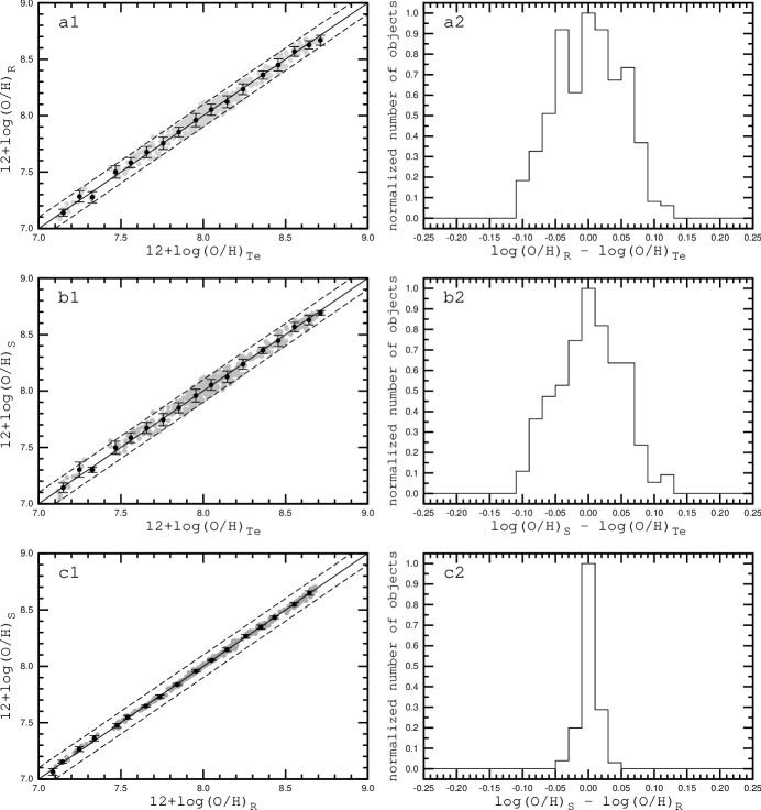
Figure 3: Panel $a1$ shows the oxygen abundance (O/H)_R as a function of oxygen abundance (O/H)${}_{T_{e}}$ for the calibrating H ii regions (313 data points). The grey points stand for individual H ii regions. The dark points represent the mean values of the abundances in bins of 0.1 dex in (O/H)${}_{T_{e}}$. The bars are the mean values of the differences of the oxygen abundances (O/H)_R and (O/H)${}_{T_{e}}$ of our H ii regions in bins. The solid line is that of equal values; the dashed lines show the $\pm 0.1$ dex deviations from unity. Panel $a2$ shows the normalized histogram of the differences between the (O/H)_R and (O/H)${}_{T_{e}}$ abundances. The panels $b1$ and $b2$ are the same as the panels $a1$ and $a2$ but for the abundances (O/H)_S and (O/H)${}_{T_{e}}$. The panels $c1$ and $c2$ are the same as the panels $a$ and $a2$ but for the abundances (O/H)_S and (O/H)_R.

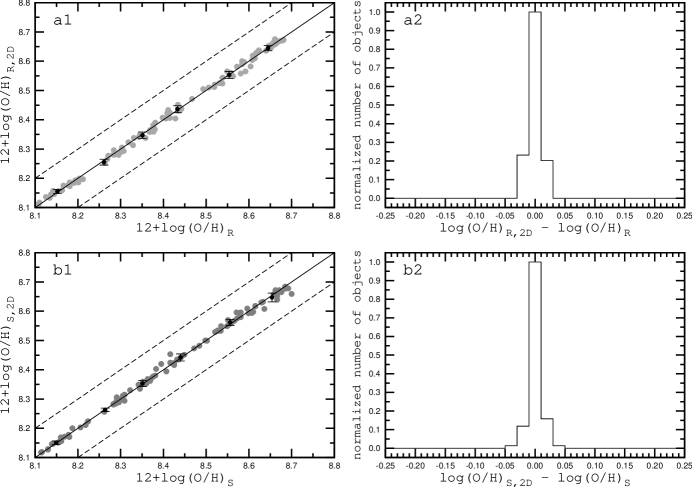
Figure 4: Panel $a1$ shows the oxygen abundance (O/H)_R,2D as a function of the oxygen abundance (O/H)_R for the calibrating H ii regions. The grey points depict the individual H ii regions. The dark points represent the mean values of the oxygen abundances in bins of 0.1 dex in (O/H)_R. The bars are the mean values of the differences between the oxygen abundances (O/H)_R,2D and (O/H)_R of our H ii regions in bins. The solid line that of equal values. The dashed lines show the $\pm$0.1 dex deviation represents equality. Panel $a2$ shows the normalized histogram of the differences between the (O/H)_R,2D and (O/H)_R abundances. The panels $b1$ and $b2$ show the same as the panels $a1$ and $a2$ but for the abundances (O/H)_S,2D and (O/H)_S.

First we consider the calibration for abundance determinations in H ii regions for the case when the $R_{2}$ line is available. A calibration of this type will be referred to as $R$ calibration. The oxygen abundance determined using such a calibration will be labeled as (O/H)_R.

The set of coefficients $a_{j}$ in Eq. 4 can be derived by imposing the condition that the average value of the differences between the oxygen abundances determined through the calibration and the original ones,

$$[(O/H)^{*}_{R}-(O/H)_{T_{e}}^{*}]^{mean}=\left(\frac{1}{n}\sum_{j=1}^{n}[(O/H)^{*}_{R,j}-(O/H)^{*}_{T_{e},j}]^{2}\right)^{1/2}$$ (5)

is minimzed for our sample of calibrating data points. The notation (O/H)^∗ $\equiv$ 12 +log(O/H) is used to allow us to write the equation in a more compact manner.

For H ii regions with log$N_{2}\geq-0.6$ (the upper branch), the following values of the coefficients were obtained: $a_{1}=8.589$, $a_{2}=0.022$, $a_{3}=0.399$, $a_{4}=-0.137$, $a_{5}=0.164$, $a_{6}=0.589$. This then results in

$$\begin{array}[]{lll}{\rm(O/H)}^{*}_{R,U}&=&8.589+0.022\,\log(R_{3}/R_{2})+0.399\,\log N_{2}\\ &+&(-0.137+0.164\,\log(R_{3}/R_{2})+0.589\log N_{2})\\ &\times&\log R_{2}\\ \end{array}$$ (9)

where (O/H)${}^{*}_{R,U}$ = 12 +log(O/H)_R,U.

For H ii regions with log$N_{2}<-0.6$ (the lower branch), the obtained values of the coefficients are: $a_{1}=7.932$, $a_{2}=0.944$, $a_{3}=0.695$, $a_{4}=0.970$, $a_{5}=-0.291$, $a_{6}=-0.019$, and

$$\begin{array}[]{lll}{\rm(O/H)}^{*}_{R,L}&=&7.932+0.944\,\log(R_{3}/R_{2})+0.695\,\log N_{2}\\ &+&(0.970-0.291\,\log(R_{3}/R_{2})-0.019\log N_{2})\\ &\times&\log R_{2}\\ \end{array}$$ (13)

where (O/H)${}^{*}_{R,L}$ = 12 +log(O/H)_R,L.

Panel $a1$ of Fig. 3 shows the oxygen abundance (O/H)_R as a function of the oxygen abundance (O/H)${}_{T_{e}}$ for the calibrating data points. The grey points mark individual H ii regions. We split our sample of H ii regions into bins of 0.1 dex in the (O/H)${}_{T_{e}}$ abundance. The mean oxygen abundances (O/H)${}_{T_{e}}^{mean}$ and (O/H)${}_{R}^{mean}$ for the H ii regions in each bin were determined. The absolute values of the mean difference between (O/H)_R and (O/H)${}_{T_{e}}$ were estimated for each bin using Eq. 5. The mean values of (O/H)${}_{T_{e}}^{mean}$ and (O/H)${}_{R}^{mean}$ are shown in panel $a1$ of Fig. 3 as dark points while the bars show the absolute values of the mean difference between the oxygen abundances (O/H)_R and (O/H)${}_{T_{e}}$ for each bin. The solid line is that of equal values; the dashed lines show the $\pm 0.1$ dex deviations from the unity line.

Panel $a2$ of Fig. 3 shows the normalized histogram of the differences between the calibration-based oxygen abundances (O/H)_R inferred here and the directly measured (O/H)${}_{T_{e}}$ values.

The examination of panels $a1$ and $a2$ of Fig. 3 shows that the oxygen abundances (O/H)_R and (O/H)${}_{T_{e}}$ agree usually within 0.1 dex. The mean difference for the 313 calibrating H ii regions is 0.049 dex. On the one hand, this suggests that our reference sample does indeed contain H ii regions with reliable oxygen abundances (O/H)${}_{T_{e}}$. On the other hand, this indicates that the chosen form of the calibration relations, Eq. 4, allows us to reproduce the relation between the oxygen abundances in an H ii region and the intensities of the strong emission lines in its spectrum rather well.

3.2.2 S calibrations

There are many measurements of H ii regions where the line $R_{2}$ is not available, for instance in the spectra of nearby galaxies in the Sloan Digital Sky Survey (SDSS). It has been argued that the oxygen abundance in an H ii region can be estimated even if the line $R_{2}$ is not available (Pilyugin & Mattsson, 2011). Now we consider the calibration for such a case. We will use the sulphur line $S_{2}$ intensity instead of the oxygen $R_{2}$ line intensity. A calibration of this type will be referred to as $S$ calibration, and the oxygen abundance determined using this kind of calibration will be labeled (O/H)_S. The same form of the calibration relation as in Eq. 4 is adopted.

Using the calibrating H ii regions of the upper branch (log$N_{2}\geq-0.6$), the following values of the coefficients $a_{j}$ were obtained: $a_{1}=8.424$, $a_{2}=0.030$, $a_{3}=0.751$, $a_{4}=-0.349$, $a_{5}=0.182$, $a_{6}=0.508$. The corresponding calibration relation is

$$\begin{array}[]{lll}{\rm(O/H)}^{*}_{S,U}&=&8.424+0.030\,\log(R_{3}/S_{2})+0.751\,\log N_{2}\\ &+&(-0.349+0.182\,\log(R_{3}/S_{2})+0.508\log N_{2})\\ &\times&\log S_{2}\\ \end{array}$$ (17)

where (O/H)${}^{*}_{S,U}$ = 12 +log(O/H)_S,U. Using the calibrating H ii regions of the lower branch (log$N_{2}<-0.6$), we obtained the following values for the coefficients $a_{j}$: $a_{1}=8.072$, $a_{2}=0.789$, $a_{3}=0.726$, $a_{4}=1.069$, $a_{5}=-0.170$, $a_{6}=0.022$. Then

$$\begin{array}[]{lll}{\rm(O/H)}^{*}_{S,L}&=&8.072+0.789\,\log(R_{3}/S_{2})+0.726\,\log N_{2}\\ &+&(1.069-0.170\,\log(R_{3}/S_{2})+0.022\log N_{2})\\ &\times&\log S_{2}\\ \end{array}$$ (21)

where (O/H)${}^{*}_{S,L}$ = 12 +log(O/H)_S,L.

Panel $b1$ of Fig. 3 shows the comparison between the oxygen abundances (O/H)_S and (O/H)${}_{T_{e}}$ for our sample of reference H ii regions. The grey points denote the values for the individual H ii regions. The dark points represent the mean oxygen abundances (O/H)${}_{T_{e}}^{mean}$ and (O/H)${}_{S}^{mean}$ for the H ii regions in bins of 0.1 dex in (O/H)${}_{T_{e}}$. The bars show the absolute values of the mean difference between the oxygen abundances (O/H)_S and (O/H)${}_{T_{e}}$ for each bin. The solid line indicates equality. The dashed lines show the $\pm$0.1 dex deviation from these equal values. In panel $b2$ of Fig. 3 we plot the normalized histogram of the differences between the calibration-based oxygen abundances (O/H)_S and the directly measued (O/H)${}_{T_{e}}$ values. Inspection of panels $b1$ and $b2$ of Fig. 3 shows that the difference between the oxygen abundances (O/H)_S and (O/H)${}_{T_{e}}$ is usually less than 0.1 dex. The mean difference for our 313 calibrating H ii regions is 0.048 dex.

Panel $c1$ of Fig. 3 shows the comparison between the oxygen abundances (O/H)_S and (O/H)_R for our calibrating data points. Panel $c2$ of Fig. 3 shows the normalized histogram of the differences between the oxygen abundances (O/H)_S and (O/H)_R. The panels $c1$ and $c2$ of Fig. 3 demonstrate that the $R$ and $S$ calibrations produce oxygen abundance values that are very close to each other. The mean difference for the 313 calibrating H ii regions amounts to only 0.013 dex.

3.2.3 Two-dimensional $R$ and $S$ calibrations for the upper branch

The calibration relations suggested above are three-dimensional, i.e., the calibration for the oxygen abundance determination involves three parameters: log($R_{3}/R_{2}$), log$N_{2}$, and log$R_{2}$, or log($R_{3}/S_{2}$), log$N_{2}$, and log$S_{2}$. It was noted above (see Fig. 2) that there is a distinct dependence of the oxygen abundance on the value of the excitation parameter $P$ at high electron temperatures (lower branch) and this dependence disappears at low temperatures (upper branch). Hence one may expect that the dependence of the oxygen abundance on the value of the excitation parameter $P$ can be neglected and two-dimensional calibrations can be determined for the upper branch.

The obtained two-dimensional $R$ relation for the upper branch is

$$\begin{array}[]{lll}12+{\rm(O/H)}_{R,2D}&=&8.589+0.329\,\log N_{2}\\ &+&(-0.205+0.549\,\log N_{2})\times\log R_{2}\\ \end{array}$$ (24)

The inferred two-dimensional $S$ relation for the upper branch is

$$\begin{array}[]{lll}12+{\rm(O/H)}_{S,2D}&=&8.445+0.699\,\log N_{2}\\ &+&(-0.253+0.217\,\log N_{2})\times\log S_{2}\\ \end{array}$$ (27)

Panel $a1$ of Fig. 4 shows the comparison between oxygen abundances for the calibrating H ii regions obtained through the three-dimensional calibration (O/H)_R and through the two-dimensional calibration (O/H)_R,2D. Panel $a2$ of Fig. 4 displays the normalized histogram of the differences between the oxygen abundances (O/H)_R,2D and (O/H)_R. The panels $b1$ and $b2$ of Fig. 4 show a similar comparison between the oxygen abundances (O/H)_S and (O/H)_S,2D. Fig. 4 demonstrates that the two-dimensional and three-dimensional $R$ and $S$ calibrations produce oxygen abundances for H ii regions of the upper branch that are in very good agreement with one another.

Thus, the oxygen abundances in high-metallicity H ii regions (the upper branch) can be estimated using the intensities of only two lines, namely $R_{2}$ and $N_{2}$ (or $S_{2}$ and $N_{2}$).

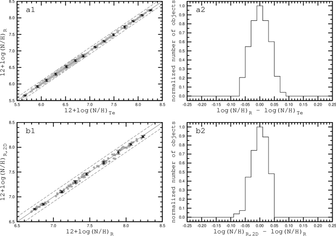
Figure 5: Panel $a1$ shows the nitrogen abundance (N/H)_R as a function of the nitrogen abundance (N/H)${}_{T_{e}}$ for the calibrating H ii regions. The grey points mark individual H ii regions. The dark points represent the mean values of the abundances in bins of 0.1 dex in (N/H)${}_{T_{e}}$. The bars denote the mean values of the differences of the oxygen abundances (N/H)_R and (N/H)${}_{T_{e}}$ of the H ii regions in bins. The solid line indicates equal values; the dashed lines show the $\pm$0.1 dex deviation from unity. Panel $a2$ contains the normalized histogram of the differences between the (N/H)_R and (N/H)${}_{T_{e}}$ abundances. The panels $b1$ and $b2$ are the same as the panels $a1$ and $a2$ but for the abundances (N/H)_R,2D and (N/H)_R.

3.3 Calibration relations for determinations of the nitrogen abundance

Here we establish calibration relations for nitrogen abundance determinations in H ii regions. Fig. 2 shows that the general behaviour of the nitrogen abundances in the considered diagrams is similar to that of the oxygen abundances. This suggests that an expression of the same form as Eq. 4 can be adopted for the calibration relation for the nitrogen abundance determinations.

Based on the H ii regions of the upper branch (log$N_{2}\geq-0.6$), the following values of the coefficients $a_{j}$ were obtained: $a_{1}=7.939$, $a_{2}=0.135$, $a_{3}=1.217$, $a_{4}=-0.765$, $a_{5}=0.166$, $a_{6}=0.449$. The resulting calibration relation for the nitrogen abundance determination is

$$\begin{array}[]{lll}{\rm(N/H)}^{*}_{R,U}&=&7.939+0.135\,\log(R_{3}/R_{2})+1.217\,\log N_{2}\\ &+&(-0.765+0.166\,\log(R_{3}/R_{2})+0.449\log N_{2})\\ &\times&\log R_{2}\\ \end{array}$$ (31)

where (N/H)${}^{*}_{R,U}$ = 12 +log(N/H)_R,U.

For the H ii regions on the lower branch (log$N_{2}<-0.6$), the values of the coefficients are: $a_{1}=7.476$, $a_{2}=0.879$, $a_{3}=1.451$, $a_{4}=-0.011$, $a_{5}=-0.327$, $a_{6}=-0.064$, and the calibration relation is

$$\begin{array}[]{lll}{\rm(N/H)}^{*}_{R,L}&=&7.476+0.879\,\log(R_{3}/R_{2})+1.451\,\log N_{2}\\ &+&(-0.011-0.327\,\log(R_{3}/R_{2})-0.064\log N_{2})\\ &\times&\log R_{2}\\ \end{array}$$ (35)

where (N/H)${}^{*}_{R,L}$ = 12 +log(N/H)_R,L.

Panel $a1$ of Fig. 5 shows the comparison between the nitrogen abundances (N/H)_R and (N/H)${}_{T_{e}}$ for our sample of calibrating H ii regions. The grey points denote the values for the individual H ii regions. The dark points represent the mean nitrogen abundances (N/H)${}_{T_{e}}^{mean}$ and (N/H)${}_{R}^{mean}$ for the H ii regions in bins of 0.2 dex in (N/H)${}_{T_{e}}$. The bars show the absolute values of the mean difference between the nitrogen abundances (N/H)_R and (N/H)${}_{T_{e}}$ for each bin. The solid line is that of equal values; the dashed lines delineate the $\pm$0.1 dex deviation from equality. Panel $a2$ of Fig. 5 shows the normalized histogram of the differences between the calibration-based nitrogen abundances (N/H)_R and the directly measured (N/H)${}_{T_{e}}$ values. The panels $a1$ and $a2$ of Fig. 5 demonstrate that the difference between the nitrogen abundances (N/H)_R and (N/H)${}_{T_{e}}$ is usually less than 0.1 dex. The mean difference for the 313 calibrating H ii regions is 0.031 dex.

A comparison of the panels $a1$ and $a2$ of Fig. 3 with the panels $a1$ and $a2$ of Fig. 5 shows that the agreement between the $R$-calibration-based and the $T_{e}$-based nitrogen abundances is better than that for the oxygen abundances. Indeed, the mean difference (N/H)_R – (N/H)${}_{T_{e}}$ is 0.031 dex while the mean difference (O/H)_R – (O/H)${}_{T_{e}}$ is 0.049 dex.

We also constructed the $S$ calibration for the determination of the nitrogen abundances. However, the nitrogen abundances estimated with the $S$ calibration are much more uncertain those produced by the $R$ calibration. Therefore we do not discuss the $S$ calibration for nitrogen abundance determinations here.

As in the case of oxygen, the two-dimensional $R$ calibration was constructed for the high-metallicity H ii regions (upper branch). We obtained the relation

$$\begin{array}[]{lll}12+{\rm(N/H)}_{R,2D}&=&7.903+0.927\,\log N_{2}\\ &+&(-0.819+0.686\,\log N_{2})\times\log(R_{2})\\ \end{array}$$ (38)

Panel $b1$ of Fig. 5 shows the comparison between the nitrogen abundances of the calibrating H ii regions obtained through the three-dimensional calibration (N/H)_R and through the two-dimensional calibration (N/H)_R,2D. Panel $b2$ of Fig. 5 displays the normalized histogram of the differences between the nitrogen abundances (N/H)_R,2D and (N/H)_R. The comparison of the panels $a1$ and $a2$ of Fig. 4 with the panels $b1$ and $b2$ of Fig. 5 shows that the abundances produced by the three- and two-dimensional $R$ calibrations agree better for oxygen than for nitrogen.

Thus, the nitrogen abundance in an H ii region can be obtained from the intensities of the strong emission lines $R_{2}$, $R_{3}$, and $N_{2}$ in its spectrum. Those abundances agree with the directly measured nitrogen abundances within $\sim 0.1$ dex. The nitrogen abundances in high-metallicity H ii regions (the upper branch) can also be estimated using the intensities of the two strong lines $R_{2}$ and $N_{2}$ only.

3.4 Calibration relation for determinations of the N/O ratio

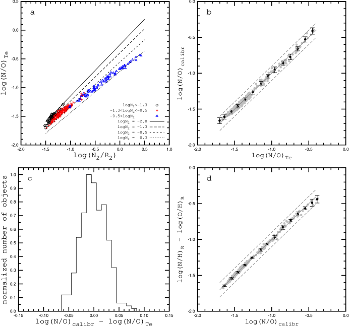
Figure 6: Panel $a$. The nitrogen-to-oxygen abundance ratio N/O as a function of the line intensity ratio N₂/R₂ for the calibrating H ii regions. H ii regions with $N_{2}$ intensities in three different intervals are shown by different symbols. The solid, dashed, and dotted lines show the calibration relation for different values of the intensity of the line $N_{2}$. Panel $b$. The nitrogen-to-oxygen abundance ratio (N/O)_calibr derived from the calibration relation (Eq. 41) as a function of nitrogen-to-oxygen abundance ratio (N/O)${}_{T_{e}}$ for the calibrating H ii regions (313 data points). The grey points stand for individual H ii regions. The dark points represent the mean values of the nitrogen-to-oxygen abundance ratios in bins of 0.1 dex in (N/O)${}_{T_{e}}$. The bars are mean values of the differences of abundance ratios (N/O)_calibr and (N/O)${}_{T_{e}}$ of our H ii regions in bins. The solid line is that of equal values; the dashed lines show the $\pm$0.1 dex deviations from unity. Panel $c$. Normalized histogram of the differences between N/O ratios derived from the calibration relation (Eq. 41) and through the $T_{e}$ method. Panel $d$. The same as the panel $b$ but for nitrogen-to-oxygen abundance ratios (N/O)_calibr derived from the NO calibration relation (Eq. 41) and nitrogen-to-oxygen abundance ratios determined as log(N/O)_R = log(N/H)_R – log(O/H)_R where nitrogen (N/H)_R and oxygen (O/H)_R abundances are determined separately from the corresponding calibration relations (Eqs. 9, 13, 31, 35).

It is interesting to also establish the expression that relates the nitrogen-to-oxygen abundance ratio N/O in an H ii region with the intensities of the strong lines in its spectrum. Panel $a$ of Fig. 6 shows the N/O ratio as a function of the line intensity ratio N₂/R₂ for our sample of reference H ii regions. The H ii regions were subdivided into three subsamples according to the intensity of the $N_{2}$ line. Those subsamples are plotted using different symbols. Panel $a$ of Fig. 6 suggests that the relation between the abundance ratio N/O and the line intensity ratio N₂/R₂ can be fitted by a linear expression for each subsample of H ii regions. The N/O – $N_{2}/R_{2}$ relations for different subsamples are shifted relative each to other and have different slopes. We derived the following calibration relation for the total sample:

$$\begin{array}[]{lll}\log{\rm(N/O)}&=&-0.657-0.201\,\log N_{2}\\ &+&(0.742-0.075\,\log N_{2})\times\log(N_{2}/R_{2})\\ \end{array}$$ (41)

The lines in panel $a$ of Fig. 6 show the calibration relation for different values of the intensity of the $N_{2}$ line.

Panel $b$ of Fig. 6 shows the nitrogen-to-oxygen abundance ratio (N/O)_calibr derived from the calibration relation (Eq. 41) as a function of the nitrogen-to-oxygen abundance ratio (N/O)${}_{T_{e}}$ for the calibrating H ii regions. The grey points mark individual H ii regions. We again split our sample of H ii regions into bins of 0.1 dex in the (N/O)${}_{T_{e}}$ abundance ratio. We determined the mean nitrogen-to-oxygen abundance ratios (N/O)${}_{T_{e}}^{mean}$ and (N/O)${}_{calibr}^{mean}$ for the H ii regions in each bin. The absolute values of the mean difference between (N/O)_calibr and (N/O)${}_{T_{e}}$ were estimated for each bin using Eq. 5. Those mean values are shown in the panel $b$ of Fig. 6 by the dark points while the bars show the absolute values of the mean difference between the nitrogen-to-oxygen abundance ratios (N/O)_calibr and (N/O)${}_{T_{e}}$ for each bin. The solid line is that of equal values, the dashed lines show the $\pm$0.1 dex deviations from the unity line.

Panel $c$ of Fig. 6 shows the normalized histogram of the differences between the N/O ratios derived from the calibration relation (Eq. 41) and through the $T_{e}$ method for our calibrating H ii regions.

Above, we constructed the calibration relations for the determination of the nitrogen and oxygen abundances. If the nitrogen and oxygen abundances are estimated separately then the nitrogen-to-oxygen abundance ratio can be easily obtained. Let us compare the nitrogen-to-oxygen abundance ratio (N/O)_calibr determined immediately from the corresponding calibration relation (Eq. 41) and the nitrogen-to-oxygen abundance ratio (N/O)_R obtained from the nitrogen (N/H)_R and oxygen (O/H)_R abundances determined separately from the corresponding relations (Eqs. 9, 13 for the oxygen abundances and Eqs. 31, 35 for the nitrogen abundances). Panel $d$ of Fig. 6 shows the comparison between the nitrogen-to-oxygen abundance ratio (N/O)_calibr and (N/O)_R.

Inspection of Fig. 6 suggests that the N/O abundance ratio in an H ii region estimated from the intensities of the two strong emission lines $N_{2}$ and $R_{2}$ agrees with the directly measured N/O abundance ratio within $\sim$0.05 dex for the bulk of our reference H ii regions. The mean difference between the N/O abundance ratios obtained from Eq. 41 and through the $T_{e}$ method is 0.026 dex for our 313 calibrating data points. The values of the nitrogen-to-oxygen abundance ratio (N/O)_calibr determined directly from the corresponding calibration relation and the nitrogen-to-oxygen abundance ratio (N/O)_R obtained from nitrogen (N/H)_R and oxygen (O/H)_R abundances determined separately are also close to each other. This suggests that our calibration relations are self-consistent.

4 Discussion and conclusions

In this study, we derived simple relations (calibrations) between the oxygen (nitrogen) abundance in H ii regions using the intensities of the strong lines in their spectra. These relations can be applied to derive nebular abundances from spectroscopic measurements that do not permit the use of the direct method for abundance determinations. The choice of more sophisticated expressions may result in an even better agreement between the calibration-based and the directly measured abundances. However, the abundances produced by the suggested calibrations agree with the measured abundances to within about 0.1 dex, which is comparable with the expected range of uncertainties in the directly measured abundances of the calibrating H ii regions. Therefore, one can expect that a significant increase of the precision of the calibration-based abundances can only be provided by a calibration based on a sample of reference H ii regions that is larger in quantity and/or higher in the quality of the abundance determinations through the direct $T_{e}$-based method as compared to the sample used here. For that purpose, new high precision measurements of H ii regions would be needed.

In the following we discuss the properties and validity of the suggested calibrations.

4.1 The transition between the upper and lower branches

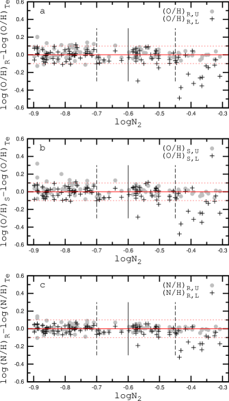
Figure 7: Comparison of the abundances in H ii regions with log$N_{2}$ near the boundary value obtained through the calibration relations for the upper and lower branches. Panel $a$. The differences between oxygen abundances estimated from the $R$ calibration for the upper branch and the direct $T_{e}$-based oxygen abundance (O/H)_R,U – (O/H)${}_{T_{e}}$ (circles) and the difference (O/H)_R,L – (O/H)${}_{T_{e}}$ (plus signs) as a function of the nitrogen line $N_{2}$ intensity. The solid vertical line marks the adopted boundary dividing the ranges of the applicability of the lower and upper branch calibration relations. The dashed vertical lines show the interval in log$N_{2}$ where both relations produce abundances that are in close agreement. Panel $b$. The same as panel $a$ but for the $S$ calibration. Panel $c$. The same as panel $a$ but for nitrogen abundances.

We constructed different calibration relations for the abundance determinations in H ii regions of the upper and lower branches. A value of log$N_{2}=-0.6$ was adopted as the condition separating the ranges of applicability of the calibration relations. H ii regions with log$N_{2}\geq-0.6$ are assumed to belong to the upper branch and objects with log$N_{2}<-0.6$ to the lower branch. This separation criterium was inferred from the examination of Fig. 2 and is somewhat arbitrary. It is important that the abundances produced by the calibrations for the lower and upper branches are compatible with each other in the boundary region separating the ranges of their applicability. Indeed, two H ii regions located close to the dividing line on both sides have similar abundances. Therefore, the abundance resulting from the lower branch calibration in an H ii region located on the one side of the boundary line should be close to the abundance produced by the upper branch calibration in an H ii region located on the other side of the dividing line. Is this the case?

We now consider H ii regions with nitrogen line $N_{2}$ intensities near the adopted boundary value, with intensities from log$N_{2}=-0.9$ to $-0.3$. As a test, the abundances in those H ii regions were obtained both with the calibration relations for the upper branch and for the lower branch. The filled grey circles in panel $a$ of Fig. 7 show the differences between the oxygen abundance estimated from the $R$ calibration for the upper branch and the direct $T_{e}$-based oxygen abundance (O/H)_R,U – (O/H)${}_{T_{e}}$ as a function of the nitrogen line $N_{2}$ intensity. The plus signs show the differences between the oxygen abundance estimated from the $R$ calibration for the lower branch and the direct $T_{e}$-based oxygen abundance (O/H)_R,L – (O/H)${}_{T_{e}}$ for the same objects. The solid vertical line shows the adopted boundary dividing the ranges of the applicability of the lower and upper branch calibration relations. The dashed vertical lines indicate the interval in log$N_{2}$ where both relations produce rather close abundances. Panel $a$ of Fig. 7 shows that the $R$ calibration for the upper branch provides rather accurate oxygen abundances for objects with log$N_{2}$ below the adopted limit, up to log$N_{2}\sim-0.7$. In turn, the $R$ calibration for the lower branch results in fairly accurate oxygen abundances for objects with log$N_{2}$ higher than the adopted limit, up to log$N_{2}\sim-0.45$, with a few exceptions. The ranges of applicability of the $R$ calibration relations for the oxygen abundance determinations overlap in the range from log$N_{2}\sim-0.7$ to $-0.45$. The dashed vertical lines show the interval in log$N_{2}$ where both relations produce abundances that are in close agreement.

Panel $b$ of Fig. 7 shows the difference (O/H)_S,U – (O/H)${}_{T_{e}}$ and (O/H)_S,L – (O/H)${}_{T_{e}}$ as a function of the $N_{2}$ nitrogen line intensity. The ranges of applicability of the $S$ calibration relations for the oxygen abundance determinations also overlap. Panel $c$ of Fig. 7 shows the difference (N/H)_R,U – (N/H)${}_{T_{e}}$ and (N/H)_R,L – (N/H)${}_{T_{e}}$ as a function of the $N_{2}$ nitrogen line intensity. Again, the ranges of applicability of the $R$ calibration relations for the nitrogen abundance determinations overlap.

Thus, the calibrations for the lower and upper branches are compatible with each other in the boundary regime dividing the ranges of their applicability. Moreover, the ranges of their applicability overlap. In practice, H ii regions with $N_{2}$ nitrogen line intensities near the adopted boundary value can be misclassified due to errors in the $N_{2}$ measurements. The H ii regions that truly belong to the upper branch with underestimated $N_{2}$ nitrogen line intensities can be classified as objects of the lower branch and vice versa. However, since the ranges of the applicability of the lower and upper branch calibration relations overlap the error in the abundance due to the misclassification of H ii regions is not large.

4.2 Verification of the calibrations: abundances in a large sample of H ii regions

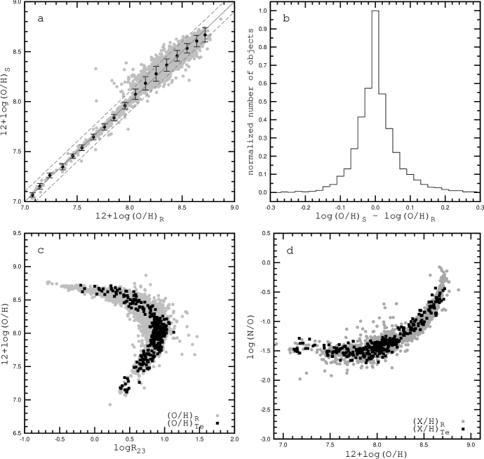
Figure 8: The application of the suggested calibrations to a large sample of 3454 spectra of H ii regions in spiral and irregular galaxies. Panel $a$. Oxygen abundance (O/H)_S vs. oxygen abundance (O/H)_R. The grey points denote individual H ii regions. The dark points represent mean abundances for objects in bins with a size of 0.1 dex in (O/H)_R. The error bars show the mean value of the differences between (O/H)_S and (O/H)_R. The solid diagonal line indicates equality; the dashed lines show the $\pm$0.1 dex offsets from equal values. Panel $b$. The normalized histogram of the differences between (O/H)_S and (O/H)_R. Panel $c$. The O/H – $R_{23}$ diagram. The grey points are the (O/H)_R abundances for the compiled sample of H ii regions. The dark squares mark the (O/H)${}_{T_{e}}$ abundances for the calibrating data points. Panel $d$. The N/O – O/H diagram. The grey points are the (X/H)_R abundances for the compiled sample. The dark squares are the (X/H)${}_{T_{e}}$ abundances for the calibrating data points.

We have compiled a large number of spectra of H ii regions in spiral and irregular galaxies in our previous studies Pilyugin et al. (2012, 2014). The $R_{2}$, $R_{3}$, $N_{2}$, and $S_{2}$ line intensity measurements are available in 3454 spectra of H ii regions. Those data provide an additional possibility to test the validity of the abundances produced by the suggested calibrations.

Panel $a$ of Fig. 8 shows the $S$-calibration-based oxygen abundances (O/H)_S as a function of $R$-calibration-based oxygen abundances (O/H)_R for the compiled sample of H ii regions. The grey points stand for individual H ii regions. The dark points represent the mean abundances for objects in bins with sizes of 0.1 dex in (O/H)_R. The error bars show the mean value of the differences between (O/H)_S and (O/H)_R in the H ii regions within each bin. Objects with large absolute values of the difference between (O/H)_S and (O/H)_R abundances (i.e., larger than 0.2 dex) were excluded in the determinations of the mean values of the abundance and mean values of the abundance differences. The solid diagonal line represents equality; the dashed lines show $\pm$0.1 dex offsets from equal values. Panel $b$ of Fig. 8 displays the normalized histogram of the differences between the (O/H)_S and (O/H)_R abundances. The panels $a$ and $b$ of Fig. 8 demonstrate that the (O/H)_S and the (O/H)_R abundances agree with each other within $\sim 0.05$ dex for the majority of the H ii regions. It should be emphasized the value of 0.05 dex cannot be interpreted as the precision of the abundance determinations with our calibration relations. The uncertainties in the $R_{3}$ and $N_{2}$ line measurements can introduce similar errors in the (O/H)_R and (O/H)_S abundances. Therefore, this abundance uncertainty cannot be revealed through the comparison between (O/H)_R and (O/H)_S abundances.

The O/H vs. $R_{23}$ diagram is a well-studied diagnostic diagram. This diagram was used to construct calibrations for oxygen abundance determinations by numerous investigators (e.g., Edmunds & Pagel, 1984; Dopita & Evans, 1986; McGaugh, 1991; Zaritsky, Kennicutt & Huchra, 1994; Pilyugin, 2000, 2001a; Pilyugin & Thuan, 2005). Panel $c$ of Fig. 8 shows the O/H – $R_{23}$ diagram. The grey points indicate the (O/H)_R abundances for our sample of compiled H ii regions. The dark squares mark the (O/H)${}_{T_{e}}$ abundances for the calibrating data points. The objects with calibration-based (O/H)_R abundances follow closely the trend traced by objects with direct (O/H)${}_{T_{e}}$ abundances.

The N/O vs. O/H diagram can be also used to test the validity of the oxygen and nitrogen abundances produced by the suggested calibrations. Many studies are devoted to the investigation of the N/O – O/H diagram (Edmunds & Pagel, 1978; Izotov & Thuan, 1999; Henry et al, 2000; Pilyugin et al., 2003, 2004; Berg et al., 2012; Annibali et al., 2015, among many others). Panel $d$ of Fig. 8 shows the N/O – O/H diagram. The grey points mark the (X/H)_R abundances for our compiled sample. The dark squares show the (X/H)${}_{T_{e}}$ abundances for the calibrating data points. Again, the objects with $R$-based abundances follow closely the trend traced by objects with direct $T_{e}$-based abundances. It is commonly accepted that the break in the N/O – O/H diagram is caused by fact that since 12 +log(O/H) $\ga 8.2$, secondary nitrogen becomes dominant and the nitrogen abundance increases at a faster rate than the oxygen abundance (Henry et al, 2000). The scatter in the N/O – O/H diagram can be caused by the time delay between nitrogen and oxygen enrichment, the local enrichment in nitrogen by Wolf-Rayet stars, and by enriched galactic winds (e.g. Edmunds & Pagel, 1978; Pilyugin, 1992, 1993; Henry et al, 2000; López-Sánchez & Esteban, 2010; Pilyugin & Thuan, 2011; Tsujimoto & Bekki, 2013; Miralles-Caballero et al., 2014).

4.3 Verification of the calibrations: abundance gradients in the galaxy M 101

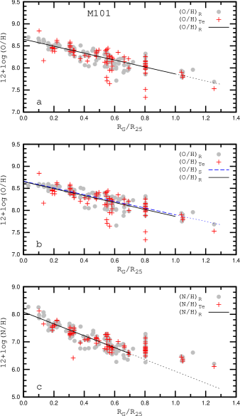
Figure 9: Panel $a$. The radial distributions of the oxygen (O/H)_R (circles) and (O/H)${}_{T_{e}}$ abundances (plus signs) across the disk of the galaxy M 101. The X-axis shows the galactocentric radius $R_{G}$ along M 101’s disk normalized by the the optical $R_{25}$ radius. The solid line indicates the linear best fit (O/H)_R = $f$($R_{G}$) to objects within the optical radius $R_{25}$. The dotted line is the extrapolation of the best fit beyond the optical radius. Panel $b$. The radial distributions of the oxygen (O/H)_S (circles) and (O/H)${}_{T_{e}}$ (plus signs) abundances. The grey (blue) dashed line shows the linear best fit (O/H)_S = $f$($R_{G}$) to the objects within the optical radius $R_{25}$, and the dotted line is its extrapolation beyond the optical radius. The solid line comes from panel $a$. Panel $c$. The radial distributions of the nitrogen (N/H)_R (circles) and (N/H)${}_{T_{e}}$ abundances (plus signs). The solid line is the linear best fit (N/H)_R = $f$($R_{G}$) to the objects with galactocentric distances less than $0.7R_{25}$, and the dotted line is its extrapolation beyond this radius.

The oxygen abundance distribution across the disk of the galaxy M 101 ($\equiv$ NGC 5457) is considered in a number of investigations (e.g., Garnett & Kennicutt, 1994; Kennicutt & Garnett, 1996; Pilyugin, 2001b; Li, Bresolin & Kennicutt, 2013). The galaxy M 101 is an attractive object to test the validity of different calibrations for two reasons. First, the auroral lines were measured in the spectra of a number of its H ii regions and, consequently, the abundances in those H ii regions could be derived through the direct $T_{e}$ method. This provides a possibility to compare the abundances produced by empirical calibrations with these direct abundances, i.e., in some sense the galaxy M 101 can be considered as a “Rosetta stone”. Second, the oxygen abundances of the H ii regions of M 101 cover a large range of abundances spanning approximately an order of magnitude. This provides a possibility to test the validity of our calibrations over the large range of abundances. Here we use emission-line measurements in 142 spectra of H ii regions in M 101 taken from Hawley (1978); Sedwick & Aller (1981); Rayo, Peimbert & Torres-Peimbert (1982); Skillman (1985); Torres-Peimbert, Peimbert & Fierro (1989); Kinkel & Rosa (1994); Garnett & Kennicutt (1994); Kennicutt & Garnett (1996); van Zee et al. (1998); Luridiana et al. (2002); Kennicutt, Bresolin & Garnett (2003); Bresolin (2007); Esteban et al. (2009); Li, Bresolin & Kennicutt (2013). It should be noted that the number of spectra is larger than the number of measured H ii regions because some H ii regions were measured several times.

Panel $a$ of Fig. 9 shows the radial distributions of the $T_{e}$-based (plus signs) and $R$-calibration-based (circles) oxygen abundances across the disk of the galaxy M 101. The solid line shows the linear best fit (O/H)_R = $f$($R_{G}$) to the objects within the optical radius $R_{25}$. The dotted line is the extrapolation of the best fit beyond the optical radius. Panel $a$ of Fig. 9 shows that the radial distribution of the $R$-calibration-based oxygen abundances follows that of the $T_{e}$-based abundances very well. The radial distributions of the oxygen abundances within and beyond the optical radius (up to $\sim 1.3R_{25}$) can be described by the unique (O/H)_R – $R_{G}$ relation.

Panel $b$ of Fig. 9 shows the radial distributions of the oxygen (O/H)_S (circles) and (O/H)${}_{T_{e}}$ (plus signs) abundances. The grey (blue) dashed line is the linear best fit (O/H)_S = $f$($R_{G}$) to the objects within the optical radius $R_{25}$, and the dotted line is its extrapolation beyond the optical radius. For comparison, the best fit to the (O/H)_R abundances is also shown by the solid line (from panel $a$). The (O/H)_S – $R_{G}$ relation is very close to the (O/H)_R – $R_{G}$ relation; in fact they coincide with each other.

Panel $c$ of Fig. 9 shows the radial distributions of the nitrogen (N/H)_R (circles) and (N/H)${}_{T_{e}}$ (plus signs) abundances. The solid line is the linear best fit (N/H)${}_{R}=f(R_{G}$) to the objects with galactocentric distances less than $0.7R_{25}$, and the dotted line is its extrapolation beyond this radius. As in the case of the oxygen abundances, the radial distribution of the $R$-calibration-based nitrogen abundances follows those of the $T_{e}$-based nitrogen abundances well. In contrast to the oxygen abundance, however, the radial distribution of the nitrogen abundances shows a break at $\sim$0.7$R_{25}$ (it is difficult to derive the exact value of the break radius because of the scatter in the nitrogen abundance at a given galactocentric distance). The slope of the radial distribution of the nitrogen abundances beyond this radius becomes shallower. This is not surprising. As we noted above, since 12 +log(O/H) $\ga 8.2$, secondary nitrogen becomes dominant and the nitrogen abundance increases at a faster rate than the oxygen abundance.

4.4 On the metallicity scale for H ii regions

For the sake of clarity we will briefly discuss the validity and reliability of the oxygen abundances. The validity and reliability of the calibration-based abundances can be addressed on three levels. Firstly, the accuracy of the calibration relations depend on the number and quality of the calibrating data points. Fig. 1 shows that the number of the reference H ii regions at high metallicities is relatively small. As was noted earlier, new high precision measurements of H ii regions, especially at high metallicities, would be desirable to increase the reliability of the calibration-based abundances. The abundances in H ii regions provided by the suggested calibration relations are in agreement with the $T_{e}$-based abundances within 0.1 dex, i.e., the relative accuracy of the calibration-based abundances are within 0.1 dex. There is no systematic discrepancy between calibration-based and $T_{e}$-based abundances. Therefore, the validity of the absolute calibration-based abundances (the potential systematic error) is, in fact, determined by the validity of the $T_{e}$-based metallicity scale for H ii regions.

Secondly, there is a discrepancy between the values of the abundance of a given H ii region derived through the $T_{e}$ method and via the model fitting using the same collisionally excited lines (see references in Section 1). The validity and reliability of abundances obtained both through model fitting as well as through the $T_{e}$ method can be questioned. On the one hand, it is pertinent to quote a passage from a review paper written by an H ii region modeller Stasínska (2004): “A widely spread opinion is that photoionization model fitting provides the most accurate abundances. This would be true if the constraints were sufficiently numerous (not only on emission line ratios, but also on the stellar content and on the nebular gas distribution) and if the model fit were perfect (with a photoionization code treating correctly all the relevant physical processes and using accurate atomic data). These conditions are never met in practice.” On the other hand, there are a number of factors that can affect $T_{e}$-based abundance determinations. It should be stressed that the underlying logic of the classical $T_{e}$ method is irreproachable. However, the practical realization of the $T_{e}$ method relies on some assumptions that can be questioned. Indeed, the equations of the $T_{e}$ method correlate the intensities of the emission lines with the electron temperature and abundances within a volume with constant conditions (electron temperature and chemical composition). In reality, possible spatial variations of the physical conditions inside an H ii region can affect the $T_{e}$-based abundance determinations.

Thirdly, usually collisionally excited lines are used for the determination of the electron temperature and abundance in H ii regions, e.g., in the $T_{e}$ method. The electron temperature of an H ii region can be also derived from the Balmer (or Paschen) jump (Peimbert, 1967), whereas the abundance of an H ii region can also be determined from optical recombination lines. Guseva et al. (2006) and Guseva et al. (2007) determined the Balmer and/or Paschen jump temperatures in a large sample of low-metallicity (12 + log(O/H) $\la 8.36$) H ii regions. They found that the temperatures of the O⁺⁺ zones determined through the equation of the $T_{e}$ method (from collisionally excited lines) do not differ, in a statistical sense, from the temperatures of the H⁺ zones determined from the Balmer and Paschen jumps although small temperature differences of the order of 3%–5% cannot be ruled out. The O⁺⁺ abundances obtained from the optical recombination lines are systematically higher (by a factor of 1.3 – 3) than the ones determined through the equation of the $T_{e}$ method from collisionally excited lines (García-Rojas & Esteban, 2007; Esteban et al., 2014, and references therein).

Different hypotheses were used to explain the discrepancy between the abundances determined from the collisionally excited lines and from the optical recombination lines. Peimbert (1967) assumed that the temperature field within the H ii region is not uniform but that there are instead the small-scale spatial temperature fluctuations inside an H ii region. If they are important then the (O/H)${}_{T_{e}}$ abundance would be a lower limit and the abundances determined from the optical recombination lines remain unaltered. Tsamis & Péquignot (2005) suggest a dual-abundance model incorporating small-scale chemical inhomogeneities in the form of hydrogen-deficient inclusions. Neither abundances determined from the collisionally excited lines nor from the optical recombination lines are reliable in this case. Nicholls, Dopita & Sutherland (2012) and Dopita et al. (2013) argue that the energy distribution of electrons in H ii regions does not follow a Maxwell distribution. In this case, abundances determined from optical recombination lines are more reliable.

Thus, at the present time there is no absolute scale for the metallicities of H ii regions. Until the problem of the discrepancy between the abundances determined in different ways is resolved, doubts about the validity and reliability of the $T_{e}$-based (and any other) metallicity scale will remain. If at some point irrefutable proof will be established that the $T_{e}$-based abundances should be adjusted then our calibration relations should be also reconsidered.

Finally, it should be noted that the $T_{e}$ method (and, consequently, our calibrations) produces the gas-phase oxygen abundance in H ii regions. Some fraction of oxygen may be embedded in dust grains. Peimbert & Peimbert (2010) have concluded that the depletion of the oxygen abundance in H ii regions can be around 0.1 dex increasing from $\sim 0.08$ dex in low-metallicity H ii regions to $\sim 0.12$ dex in high-metallicity H ii regions. When this effect is taken into account the total (gas + dust) oxygen abundance in an H ii region is higher by $\sim 0.1$ dex than the one produced by the $T_{e}$ method and our calibrations.

5 Summary

We derive simple expressions relating the oxygen abundance in H ii regions with the intensities of the three strong lines $R_{2}$, $R_{3}$, and $N_{2}$ ($R$ calibrations) or $S_{2}$, $R_{3}$, and $N_{2}$ ($S$ calibration). We also present the $R$ calibration for nitrogen abundance determinations. We use a sample of 313 reference H ii regions with $T_{e}$-based oxygen abundances obtained originally for the counterpart method ($C$ method) as a sample of calibrating data points.

H ii regions are usually divided in two classes: the high-metallicity objects (the “upper branch”) and low-metallicity objects (the “lower branch”). We adopt a value of log$N_{2}=-0.6$ as boundary between the upper and lower branches. In other words, H ii regions with log$N_{2}\geq-0.6$ belong to the upper branch and H ii regions with log$N_{2}<-0.6$ are lower branch objects. We derive different calibration relations for the abundance determinations in H ii regions on the lower and upper branches. The ranges of the applicability of the calibration relations for the upper and lower branches overlap in the boundary region within a range of $-0.7\la$ log$N_{2}\la-0.45$.

The oxygen and nitrogen abundances estimated through the calibrations agree with the $T_{e}$-based abundances within $\sim 0.1$ dex over the whole metallicity range of H ii regions, i.e., the relative accuracy of the calibration-based abundances is 0.1 dex. The oxygen and nitrogen abundances in the high-metallicity H ii regions (upper branch) can be estimated using only the intensities of the two strong lines $R_{2}$ and $N_{2}$ (or $S_{2}$ and $N_{2}$ for oxygen).

The validity of the suggested calibrations was tested using a compilation of more than three thousand spectra of H ii regions. The locations of the calibration-based abundances in those H ii regions in the $R_{23}$ – O/H and the N/O – O/H digrams follow well the general trends traced by H ii regions with $T_{e}$-based abundances. Also, the radial distributions of the calibration-based oxygen and nitrogen abundances across the disk of the well-studied galaxy M 101 follow those of the $T_{e}$-based abundances.

We emphasize that there are two important advantages of our new calibrations in comparison to the existing ones. Firstly, in our approach, the oxygen abundances (O/H)_R and (O/H)_S – produced by two different calibrations (based on different sets of strong emission lines) – agree within $\sim 0.05$ dex for the majority of the H ii regions. It should be noted that the value of 0.05 dex cannot be interpreted as the accuracy of the abundance determinations through our calibration relations. Uncertainties in the $R_{3}$ and $N_{2}$ line measurements can introduce similar errors in the (O/H)_R and (O/H)_S abundances. Therefore, such uncertainties in the abundance cannot be revealed through the comparison between (O/H)_R and (O/H)_S abundances. Secondly, since the ranges applicability of the calibration relations for the upper and lower branches overlap the problem with the abundance determinations in the “transition” zone does not appear.

References

- Alloin et al. (1979) Alloin D., Collin-Souffrin S., Joly M., Vigroux L., 1979, A&A, 78, 200
- Andrievsky et al. (2002) Andrievsky S. M., Kovtyukh V. V., Luck R. E., Lépine J.R.D., Maciel W.J., Beletsky Y.V., 2002, A&A, 392, 491 Andrievsky, S. M.; Kovtyukh, V. V.; Luck, R. E.; Lépine, J. R. D.; Maciel, W. J.; Beletsky, Yu. V.
- Annibali et al. (2015) Annibali F., Tosi M., Pasquali A., Aloisi A., Mignoli M., Romano D., 2015, AJ, 150, 143
- Berg et al. (2012) Berg D.A., Skillman E.D., Marble A.R., et al., 2012, ApJ, 754, 98
- Blanc et al. (2015) Blanc G.A., Kewley L., Vogt F.P.A., Dopita M.A., 2015, ApJ, 798, 99
- Boeche et al. (2013) Boeche C., Siebert A., Piffl T., et al. 2013, A&A, 559, A59
- Boeche et al. (2014) Boeche C., Siebert A., Piffl T., et al. 2014, A&A, 568, A71
- Bresolin (2007) Bresolin F., 2007, ApJ, 656, 186
- Bresolin et al. (2009) Bresolin F., Gieren W., Kudritzki R.-P., Pietrzyński G., Urbaneja M.A., Carraro G., 2009, ApJ, 700, 309
- Campbell, Terlevich & Melnick (1986) Campbell A., Terlevich R., Melnick J., 1986, MNRAS, 223, 811
- Chen et al. (2003) Chen L., Hou J. L., Wang J. J. 2003, AJ, 125, 1397
- Cioni (2009) Cioni M.-R. L. 2009, A&A, 506, 1137
- Dinerstein (1990) Dinerstein H. L. 1990, in The Interstellar Medium in Galaxies, ed. H. A Thronson Jr. & J. M. Shull (Astrophysics and Space Science Library, Vol. 161; Dordrecht: Kluwer), 257
- Dopita & Evans (1986) Dopita M.A., Evans I.N., 1986, ApJ, 307, 431
- Dopita et al. (2013) Dopita M.A., Sutherland R.S., Nicholls D.C., Kewley L.J., Vogt F.P.A., 2013, ApJS, 208, 10
- Edmunds & Pagel (1978) Edmunds M.G., Pagel B.E.J., 1978, MNRAS, 185, 77
- Edmunds & Pagel (1984) Edmunds M.G., Pagel B.E.J., 1984, MNRAS, 211, 507
- Erb et al. (2006) Erb D. K., Shapley A. E., Pettini M., Steidel C. C., Reddy N. A., Adelberger K. L., 2006, ApJ, 644, 813
- Esteban et al. (2009) Esteban C., Bresolin F., Peimbert M., García-Rojas J., Peimbert A., Mesa-Delgado A., 2009, ApJ, 700, 654
- Esteban et al. (2014) Esteban C., García-Rojas J., Carigi L., Peimbert M., Bresolin F., López-Sánchez A.R., Mesa-Delgado A., 2014, MNRAS, 443, 624
- García-Rojas & Esteban (2007) García-Rojas J., Esteban C., 2007, ApJ, 670, 457
- Garnett (1992) Garnett D.R., 1992, AJ, 103, 1330
- Garnett & Kennicutt (1994) Garnett D.R., Kennicutt R.C., 1994, ApJ, 426, 123
- Grebel et al. (2003) Grebel E. K., Gallagher J. S., III, Harbeck D. 2003, AJ, 125, 1926
- Guseva et al. (2006) Guseva N.G., Izotov Y.I., Thuan T.X., 2006, ApJ, 644, 890
- Guseva et al. (2007) Guseva N.G., Izotov Y.I., Papaderos P., Fricke K.J., 2007, A&A, 464, 885
- Harbeck et al. (2001) Harbeck D., Grebel E. K., Holtzman J., et al. 2001, AJ, 122, 3092
- Haschke et al. (2012) Haschke R., Grebel E. K., Duffau S., Jin S. 2012, AJ, 143, 48
- Hawley (1978) Hawley S.A., 1978, ApJ, 224, 417
- Henry et al (2000) Henry R.B.C., Edmunds M.G., Köppen J., 2000, ApJ, 541, 660
- Izotov & Thuan (1999) Izotov Y.I., Thuan T.X., 1999, ApJ, 511, 639
- Izotov et al. (2015) Izotov Y. I., Guseva N. G., Fricke K. J., Henkel C. 2015, MNRAS, 451, 2251
- Janes (1979) Janes K. A. 1979, ApJS, 39, 135
- Kennicutt & Garnett (1996) Kennicutt R.C., Garnett D.R., 1996, ApJ, 456, 504
- Kennicutt, Bresolin & Garnett (2003) Kennicutt R.C., Bresolin F., Garnett D.R., 2003, ApJ, 591, 801
- Kewley & Dopita (2002) Kewley L.J., Dopita M.A., 2002, ApJS, 142, 35
- Kewley & Ellison (2008) Kewley L.J., Ellison S.L., 2008, ApJ, 681, 1183
- Kinkel & Rosa (1994) Kinkel U., Rosa M.R., 1994, A&A, 282, L37
- Lequeux et al. (1979) Lequeux J., Peimbert M., Rayo J. F., Serrano A., Torres-Peimbert S. 1979, A&A, 80, 155
- Li, Bresolin & Kennicutt (2013) Li Y., Bresolin F., Kennicutt R.C., 2013, ApJ, 766, 17
- López-Sánchez & Esteban (2010) López-Sánchez Á.R., Esteban C., 2010, A&A, 517, A85
- López-Sánchez et al. (2012) López-Sánchez Á.R., Dopita M.A., Kewley L.J., Zahid H.J., Nicholls D.C., Scharwächter J. 2012, MNRAS, 426, 2630
- Luridiana et al. (2002) Luridiana V., Esteban C., Peimbert M., Peimbert A., 2002, Rev. Mex. A.A., 38, 97
- Maciel & Quireza (1999) Maciel W. J., & Quireza C. 1999, A&A, 345, 629
- Marino et al. (2013) Marino R.A., Rosales-Ortega F.F., Sánchez S.F., et al., 2013, A&A, 559, A114
- McCall, Rybski & Shields (1985) McCall M.L., Rybski P.M., Shields G.A., 1985, ApJS, 57, 1
- McGaugh (1991) McGaugh S.S., 1991, 380, 140
- Mehlert et al. (2003) Mehlert D., Thomas D., Saglia R. P., Bender R., Wegner G. 2003, A&A, 407, 423
- Miralles-Caballero et al. (2014) Miralles-Caballero D., Rosales-Ortega F.F., Díaz A.I., Otí-Floranes H., Pérez-Montero E., Sánchez S.F., 2014, MNRAS, 445, 3803
- Morales-Luis et al. (2014) Morales-Luis A.B., Pérez-Montero E., Sánchez A.J., Muñoz-Muñón C., 2014, ApJ, 797, 81
- Moustakas et al. (2010) Moustakas J., Kennicutt R.C., Tremonti C.A., Dale D.A., Smith J.-D.T., Calzetti D., 2010. ApJS, 190, 233
- Nicholls, Dopita & Sutherland (2012) Nicholls D.C., Dopita M.A., Sutherland R.S., 2012, ApJ, 752, 148
- Pagel et al. (1979) Pagel B.E.J., Edmunds M.G., Blackwell D.E., Chun M.S., Smith G., 1979, MNRAS, 189, 95
- Panter et al. (2008) Panter B., Jimenez R., Heavens A. F., Charlot S. 2008, MNRAS, 391, 1117
- Peimbert (1967) Peimbert M., 1967, ApJ, 150, 825
- Peimbert & Peimbert (2010) Peimbert A., Peimbert M., 2010, ApJ, 724, 791
- Peng & Maiolino (2014) Peng Y.-J., & Maiolino R. 2014, MNRAS, 438, 262
- Pettini & Pagel (2004) Pettini M., Pagel B.E.J., 2004, MNRAS, 348, L59
- Pilyugin (1992) Pilyugin L.S., 1992, A&A, 260, 58
- Pilyugin (1993) Pilyugin L.S., 1993, A&A, 277, 42
- Pilyugin (2000) Pilyugin L.S., 2000, A&A, 362, 325
- Pilyugin (2001a) Pilyugin L.S., 2001a, A&A, 369, 594
- Pilyugin (2001b) Pilyugin L.S., 2001b, A&A, 373, 56
- Pilyugin (2003) Pilyugin L.S., 2003, A&A, 399, 1003
- Pilyugin et al. (2003) Pilyugin L.S., Thuan T.X., Vílchez J.M., 2003, A&A, 397, 487
- Pilyugin et al. (2004) Pilyugin L.S., Contini T., Vílchez J.M., 2004, A&A, 423, 427
- Pilyugin & Thuan (2005) Pilyugin L.S., Thuan T.X., 2005, ApJ, 631, 231
- Pilyugin et al. (2010) Pilyugin L.S., Vílchez J.M., Thuan T.X., 2010, ApJ, 720, 1738
- Pilyugin & Mattsson (2011) Pilyugin L.S., Mattsson L., 2011, MNRAS, 412, 1145
- Pilyugin & Thuan (2011) Pilyugin L.S., Thuan T.X., 2011, ApJ, 726, 23P
- Pilyugin et al. (2012) Pilyugin L.S., Grebel E.K., Mattsson L., 2012, MNRAS, 424, 2316
- Pilyugin et al. (2013) Pilyugin L.S., Lara-López M.A., Grebel E.K., Kehrig C., Zinchenko I.A., López-Sánchez Á.R., Vílchez J.M., Mattsson L., 2013, MNRAS, 432, 1217
- Pilyugin et al. (2014) Pilyugin L.S., Grebel E.K., Kniazev A.Y., 2014, AJ, 147, 131
- Pilyugin et al. (2015) Pilyugin, L. S., Grebel, E. K., & Zinchenko, I. A. 2015, MNRAS, 450, 3254
- Rayo, Peimbert & Torres-Peimbert (1982) Rayo J.F., Peimbert M., Torres-Peimbert S., 1982, ApJ, 255, 1
- Sánchez et al. (2013) Sánchez S. F., Rosales-Ortega F. F., Jungwiert B., et al. 2013, A&A, 554, A58
- Searle (1971) Searle L. 1971, ApJ, 168, 327
- Sedwick & Aller (1981) Sedwick K.E., Aller L.H., 1981, Proc. Nat. Acad. Sci. USA., 78, 1994
- Skillman (1985) Skillman E.D., 1985, ApJ, 290, 449
- Stasínska (2004) Stasinska G., 2004, in Cosmochemistry: The Melting Pot of the Elements, ed. C.Esteban, R.J. García López, A.Herrero and F.Sánchez (Cambridge: Cambridge Univ. Pres), 115
- Stasínska (2006) Stasinska G., 2006, A&A, 454, L127
- Thuan et al. (2010) Thuan T.X., Pilyugin L.S., Zinchenko I.A., 2010, ApJ, 712, 1029
- Torres-Peimbert, Peimbert & Fierro (1989) Torres-Peimbert S., Peimbert M., Fierro J., 1989, ApJ, 345, 186
- Tremonti et al. (2004) Tremonti C.A., et al., 2004, ApJ, 613, 898
- Tsamis & Péquignot (2005) Tsamis Y.G., Péquignot D., 2005, MNRAS, 364, 687
- Tsujimoto & Bekki (2013) Tsujimoto T., Bekki K., 2013, MNRAS, 436, 1191
- van Zee et al. (1998) van Zee L., Salzer J.J., Haynes M.P., O‘Donoghue A.A., Balonek T.J., 1998, AJ, 116, 2805
- Zahid et al. (2012) Zahid H. J., Bresolin F., Kewley L. J., Coil A. L., Davé, R. 2012, ApJ, 750, 120
- Zahid et al. (2014) Zahid H. J., Dima G. I., Kudritzki R.-P., Kewley L. J., Geller M. J., Hwang H. S., Silverman J. D., Kashino D., 2014, ApJ, 791, 130
- Zaritsky, Kennicutt & Huchra (1994) Zaritsky D., Kennicutt R.C., Huchra, J.P., 1994, ApJ, 420, 87
- Zinchenko et al. (2016) Zinchenko I.A., Pilyugin L.S., Grebel E.K., Sánchez S.F., Vílchez J.M., 2016, MNRAS, submitted