Finding Outliers in Surface Data and Video

Abstract

Surface, image and video data can be considered as functional data with a bivariate domain. To detect outlying surfaces or images, a new method is proposed based on the mean and the variability of the degree of outlyingness at each grid point. A rule is constructed to flag the outliers in the resulting functional outlier map. Heatmaps of their outlyingness indicate the regions which are most deviating from the regular surfaces. The method is applied to fluorescence excitation-emission spectra after fitting a PARAFAC model, to MRI image data which are augmented with their gradients, and to video surveillance data.

Keywords: Adjusted outlyingness, Functional data, Image data, Multiway, Robustness.

1 Introduction

The most common type of functional data are curves, typically measured over time. Also spectral data, measured over a range of wavelengths, can be considered as functional data and can be analyzed as such (Saeys et al.,, 2008). When several measurements are taken at each time point, we obtain multivariate functional data. Bivariate examples are height and weight curves of children, temperature and dewpoint temperature at several weather stations during several days, or measurements of the human heart activity at two different places on the body (Claeskens et al.,, 2014). Whereas the domain of these data is always univariate, the response can thus be multivariate.

Surface data are an increasingly common data type in several fields of research. In chemistry for example, fluorescence spectroscopy is a well known technique that yields surface data with an excitation and an emission dimension. In geography, surface data is obtained by measuring characteristics such as daily precipitation on a certain area of land. Also digital image and video data are represented by a grid of pixels and typically contain grayscale values or three-dimensional RGB values that define the color intensities. All these advanced data types can thus be seen as multivariate functional data with a bivariate domain.

To detect outlying surfaces or to flag outlying parts of a surface, it is well known that classical statistical techniques are not trustworthy as the analysis itself may be distorted by the outliers. Outlier detection for multivariate functional data with a univariate domain has been studied in depth in Hubert et al., 2015a . In that paper a taxonomy of outlying curves was proposed, and distribution-free statistical methods were introduced to measure their degree of outlyingness. Hubert et al., 2015b illustrated this on a raw excitation-emission fluorescence dataset, and proposed the functional outlier map (FOM) as a graphical display to visualize the functions according to their degree and type of outlyingness.

In this paper, we build on these methods with a threefold objective. First, we propose a cutoff to distinguish between the outlying and the regular surfaces, which makes the FOM more informative. Secondly, we improve the outlier detection ability for surface data by first modeling the data according to a multiway model and applying the FOM to the residuals instead of the raw data. Finally, we illustrate the extension of these techniques to multivariate image and video data.

The next section introduces the methodology behind the FOM as well as our new outlier detection rule. In Section 3 we apply the new rule to excitation-emission matrices before and after fitting a PARAFAC model to them. Section 4 demonstrates the performance of our method on MRI image data and introduces the idea of including gradients in the analysis. In Section 5 we apply the methodology to a video consisting of 633 color images.

2 Methodology

2.1 Functional Adjusted Outlyingness

The main concept for measuring the degree of outlyingness is the adjusted outlyingness (AO) of Brys et al., (2005). Its construction is recalled in the Appendix. For univariate data, the AO is a robust version of the absolute $z$-score as it measures an observation’s deviation from the median. It allows for skewness in the data by estimating scale separately on either side of the median. For multivariate data, the AO of a point is defined as its maximal univariate AO when projecting the data on many directions.

To extend the AO to multivariate functional data, Hubert et al., 2015a defined the functional adjusted outlyingness (fAO) of a $p$-dimensional curve $X$ as the (weighted) average of its AO values over all points of its domain. More precisely, let$\bm{Y}=\{Y_{1},Y_{2},\ldots,Y_{n}\}$ be a sample of $p$-dimensional curves, recorded at time points $\{t_{1},\ldots,t_{T}\}$. The fAO of $X$ with respect to $\bm{Y}$ is then defined as

$$\text{fAO}(X;\bm{Y})=\sum_{j=1}^{T}{\text{AO}(X(t_{j});\bm{Y}(t_{j}))\;W(t_{j})}$$ (1)

where $\bm{Y}(t_{j})$ is a sample in $p$ dimensions and $W(.)$ is a weight function for which $\sum_{j=1}^{T}{W(t_{j})}=1$. This weight function allows to assign a different importance to the outlyingness of a curve at different time points. One could for example downweight time points near the boundaries if measurements are recorded less precisely at the beginning and the end of the process.

Definition (1) for functional data with a univariate domain can easily be extended to functions with a bivariate domain such as surfaces and images. We then assume that the outcome of the experiment is recorded at a grid of discrete points, e.g. discrete excitation and emission wavelengths. Therefore, it is convenient to use two indices $j=1,\ldots,J$ and $k=1,\ldots,K$, one for each dimension of the grid, to characterize these points. A surface or image can then be represented by a $J\times K$ matrix where each cell $(j,k)$ contains the height of the surface or the color intensity at that grid point. We then define the functional adjusted outlyingness of a multivariate function $X$ with bivariate domain relative to a dataset $\bm{Y}$ of functions recorded at grid points $\{(j,k);j=1,\ldots,J\mbox{ and }k=1,\ldots,K\}$ as

$$\text{fAO}(X;\bm{Y})=\sum_{j=1}^{J}{\sum_{k=1}^{K}{\text{AO}(X(j,k);\bm{Y}(j,k))\;W_{jk}}}$$ (2)

with $\sum_{j=1}^{J}\sum_{k=1}^{K}W_{jk}=1$. For illustrative purposes we will use a uniform weight function throughout this paper, i.e. $W_{jk}=1/(JK)$ for all $j=1,\ldots,J$ and $k=1,\ldots,K$. Definition (2) can trivially be extended to functions with a multivariate domain of dimension $d>2$, such as three-dimensional images consisting of voxels.

The fAO can be applied to raw data, but in other applications it might be interesting to first fit a parametric model to the data, after which the fAO can be computed on the residuals. For multiway data, PARAFAC is a commonly used method to fit a trilinear model. The concept of applying fAO to the residuals of a PARAFAC model is illustrated on a real data example in Section 3.

When analyzing curves, it is often informative to consider the derivative of the curves as well. In particular, this is helpful when the goal is to detect curves with a deviating shape, see Hubert et al., 2015a for some examples. For surfaces or images, we can augment the available raw data by including gradients instead. This idea will be illustrated in Section 4.

2.2 Functional outlier map

The functional outlier map (FOM) was introduced in (Hubert et al., 2015b, ) as a graphical tool to visualize the degree of outlyingness of curves. A similar definition can be applied to surfaces or images. The FOM is a scatter plot which displays each function’s fAO on the horizontal axis and vAO, a measure of the variability of its AO over all points of the domain, on the vertical axis. More precisely, for each $Y_{i}$ the vAO is defined as

$$\text{vAO}(Y_{i};\bm{Y})=\text{stdev}_{j,k}(\text{AO}(Y_{i}(j,k);\bm{Y}(j,k)))/(1+\text{fAO}(Y_{i};\bm{Y}))$$ (3)

so the FOM is a scatter plot of the points

$$\left(\;\text{fAO}(Y_{i};\bm{Y}),\text{vAO}(Y_{i};\bm{Y})\;\right)$$ (4)

for $i=1,\ldots,n$. We divide by fAO in Equation (3) in order to measure relative instead of absolute variability. This can be understood as follows. Suppose that the functions are centered around zero and that $Y_{l}(j,k)=2\;Y_{i}(j,k)$ for all $j$ and $k$. Then $\text{stdev}_{j,k}(\text{AO}(Y_{l}(j,k);\bm{Y}(j,k)))=2\;\text{stdev}_{j,k}(\text{AO}(Y_{i}(j,k);\bm{Y}(j,k)))$ but their relative variability is the same. Because $\text{fAO}(Y_{l};\bm{Y})=2\;\text{fAO}(Y_{i};\bm{Y})$, dividing by fAO solves this problem.

The objective of the FOM is to reveal outliers in the data, and its interpretation is fairly straightforward. We use the taxonomy of functional outliers presented by Hubert et al., 2015a to distinguish between different types of outliers. Points in the lower left part of the FOM represent regular surfaces which hold a central position in the dataset. Points in the lower right part are surfaces with a high fAO but a low variability of their AO values. This happens for shift outliers, i.e. surfaces which have the same shape as the majority but are shifted on the whole domain. Points in the upper left part have a low fAO but a high vAO. Typical examples are isolated outliers, i.e. surfaces which only display outlyingness over a small part of their domain. The points in the upper right part of the FOM have both a high fAO and a high vAO. These correspond to surfaces which are strongly outlying on a substantial part of their domain.

In this paper we add an additional feature to the FOM, namely a rule to flag the outliers. For this purpose we define a summary measure, the combined functional outlyingness (CFO) of a surface $Y_{i}$ as

$$\text{CFO}_{i}=\text{CFO}(Y_{i};\bm{Y})=\sqrt{(\text{fAO}_{i}/\mathop{\mbox{med}}(\text{fAO}))^{2}+(\text{vAO}_{i}/\mathop{\mbox{med}}(\text{vAO}))^{2}}$$ (5)

where $\text{fAO}_{i}=\text{fAO}(Y_{i};\bm{Y})$, $\mathop{\mbox{med}}(\text{fAO})=\text{median}(\text{fAO}_{1},\ldots,\text{fAO}_{n})$ and similarly forvAO. Note that the CFO characterizes the points on the FOM through their Euclidean distance to the origin, after scaling. We expect outliers to have a large CFO. In general, the distribution of the CFO is unknown but skewed to the right. To define a cutoff, we first symmetrize the CFO by the logarithmic transformation. Then we center and scale the resulting values in a robust way and compare them with a high quantile of the gaussian distribution. More precisely, let $\text{LCFO}_{i}=\log(0.1+\text{CFO}_{i})$ for all $i=1,\ldots,n$. Then we flag function $Y_{i}$ as an outlier if

$$\frac{\text{LCFO}_{i}-\mathop{\mbox{med}}(\text{LCFO})}{\text{MAD}(\text{LCFO})}>\Phi^{-1}(0.995)\,.$$ (6)

In the denominator, MAD denotes the median absolute deviation defined as$\text{MAD}(\text{LCFO})=1.4826\;\mathop{\mbox{med}}(|\;\text{LCFO}-\mathop{\mbox{med}}(\text{LCFO})|)$.

In addition to the FOM, it is often instructive to plot the AO values themselves over their domain. For a function with a bivariate domain, this yields a two-dimensional heatmap. These plots can reveal particularly outlying regions and provide more insight into why certain surfaces are flagged as outliers by the FOM. This will be illustrated in the following sections.

3 Surface data

The Dorrit dataset contains excitation-emission landscapes of 27 mixtures of 4 fluorophores in an aqueous solution and has been studied extensively by Engelen et al., (2007), Engelen and Hubert, (2011) and Hubert et al., (2012). Such landscapes are typically stored in excitation-emission matrices (EEM). These matrices contain measurements of fluorescence intensity for 116 emission spectra ranging from 250 to 482 nm at 18 excitation wavelengths ranging from 230 to 315 nm. This yields 27 samples $Y_{i}$, each containing measurements $Y_{i}(j,k)$ for $j=1,\ldots,J=18$ and $k=1,\ldots,K=116$. Raman and Rayleigh scattering, showing up in Figure 1(a) as two diagonal ridges in landscape 8, are a common problem in this type of experiment and can severely distort the analysis. To resolve this we used the method of Engelen et al., (2007) which automatically identifies the scattering. After setting the scattering to missing values, we imputed them by interpolating each excitation profile. The result of this process is illustrated in Figure 1(b).

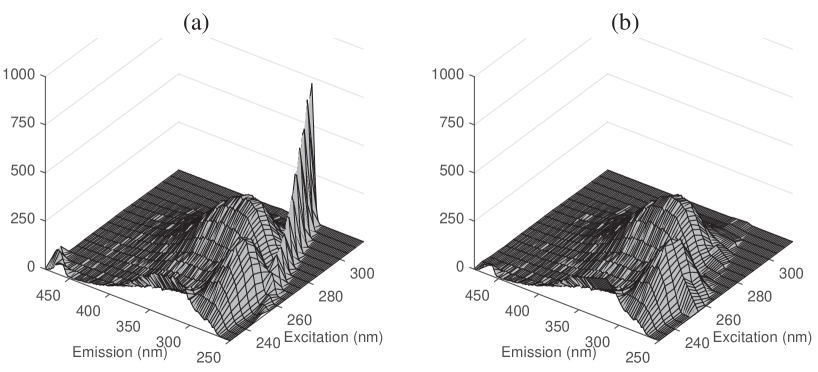
Figure 1: (a) Original landscape 8 with scatter and (b) with scatter removed.

Using Definition (2) with a uniform weight function, we obtain the functional outlier map depicted in Figure 2. The dashed black line is determined by the cutoff value (6) and shows the boundary between the regular data and the outliers. The outliers, plotted as red squares, are landscapes 3 and 5.

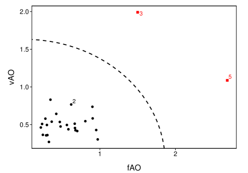
Figure 2: FOM of the raw Dorrit data.

We can improve our analysis by incorporating more information, for example by applying parallel factor analysis (PARAFAC) to the data. PARAFAC is known to be a powerful tool for analyzing multiway data and can in particular be used to decompose three-way EEM data into a trilinear model. This trilinear model states that the value of a landscape $Y_{i}$ at EE-point $(j,k)$ can be written as the product of three corresponding values of the score matrix $A$ and the loading matrices $B$ and $C$, plus an error term:

$$Y_{i}(j,k)=\sum_{f=1}^{F}{a_{if}b_{jf}c_{kf}}+e_{ijk}\;.$$ (7)

Here $F$ denotes the number of components which we take as $F=4$, corresponding to the 4 known fluorophores present in the mixtures. Applying PARAFAC to the data results in 27 residual landscapes $\widetilde{Y}_{i}(j,k)=e_{ijk}$. With the objective of outlier detection in mind, it is important to use a robust PARAFAC algorithm as it is well known that the presence of outliers can severely impact the PARAFAC decomposition. We have used the robust PARAFAC algorithm proposed by Engelen and Hubert, (2011) in which we set the robustness parameter $h=0.75$. This parameter indicates that the PARAFAC model is based on the $75\%$ of surfaces which yield the smallest residuals.

By computing the fAO on the residuals instead of the original data, the trilinear structure of the dataset is taken into account. The resulting functional outlier map is shown in Figure 3 and flags landscapes 2, 3 and 5. These outliers were also detected in Engelen and Hubert, (2011). Note that points 3 and 5 lie much further from the boundary (the dashed black curve) than in the FOM of Figure 2. This indicates that surfaces 3 and 5 have outlying values but mostly expose an outlying structure. Landscape 2 barely contains abnormally low or high values but has large residuals with respect to the PARAFAC model fitted to the majority of EEM landscapes.

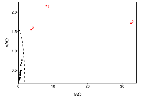
Figure 3: FOM of the residuals of the Dorrit data.

A heatmap of the AO values over the domain allows us to inspect surface 2 in more detail. Figure 4(a) plots the AOs of the original landscape 2, whereas Figure 4(b) shows the AOs of its PARAFAC residuals. To improve visibility, all AO values of 15 or higher received the darkest color. The left plot indicates that landscape 2 indeed does not have large outlying regions, as the vast majority of its cells are light-colored. However, the right plot shows that its residuals are significantly outlying in the emission spectra between 275 and 350 nm. This indicates that the shape of landscape 2 differs strongly from the shape predicted by the PARAFAC model. Therefore, this landscape can be classified as a shape outlier.

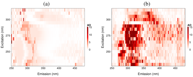
Figure 4: Heatmap of the AO values of landscape 2 for (a) the raw values, (b) the residuals after a robust PARAFAC fit.

4 Image data

The MRI dataset contains brain imaging data of 416 persons, aged between 18 and 96 years (Marcus et al.,, 2007) and can be freely accessed at www.oasis-brains.org. For each person, multiple MRI scans are available including 3 to 4 raw MRI images and several processed scans such as an averaged image of the raw scans, the atlas-registered gain field-corrected image and a masked version of the latter scan resampled to 1mm isotropic pixels. Masking sets all non-brain pixels to an intensity value of zero. Moreover these images are normalized, meaning that the size of the head is exactly the same in each image. The masked images have 176 by 208 pixels with grayscale values between 0 and 255. All together we thus have 416 observed images $Y_{i}$ containing univariate intensity values $Y_{i}(j,k)$, where $j=1,\ldots,J=176$ and $k=1,\ldots,K=208$.

There is more information in the image than just the raw values. We can incorporate part of the shape information by computing the gradient in every pixel of the image. This gradient is composed of the derivatives in the horizontal and the vertical direction. More precisely, the gradient in pixel $(j,k)$ is defined as the 2-dimensional vector $\nabla Y_{i}(j,k)=\left(\frac{\delta Y_{i}(j,k)}{\delta j},\frac{\delta Y_{i}(j,k)}{\delta k}\right)$. In practice we do not have the exact derivatives of the image at the recorded pixels, so we have to rely on numerical approximations. We use forward and backward finite differences to approximate the derivatives in the pixels at the boundary of the brain. For the other pixels, we have used central differences. In the horizontal direction these are given by

$$\frac{\delta Y_{i}(j,k)}{\delta j}\approx \frac{-3\,Y_{i}(j,k)+4\,Y_{i}(j+1,k)-Y_{i}(j+2,k)}{2} (\text{forward difference})$$

$$\frac{\delta Y_{i}(j,k)}{\delta j}\approx \frac{Y_{i}(j+1,k)-Y_{i}(j-1,k)}{2} (\text{central difference})$$

$$\frac{\delta Y_{i}(j,k)}{\delta j}\approx \frac{Y_{i}(j-2,k)-4\,Y_{i}(j-1,k)+3\,Y_{i}(j,k)}{2} (\text{backward difference}).$$

The derivatives in the vertical direction are computed analogously.

Adding these derivatives to the data yields a multiway dataset of dimensions $416\times 176\times 208\times 3$, so each $Y_{i}(j,k)$ is trivariate. For each person we thus have three data matrices which represent the original MRI image and its derivatives in both directions. Figure 5 represents these three matrices for person 144.

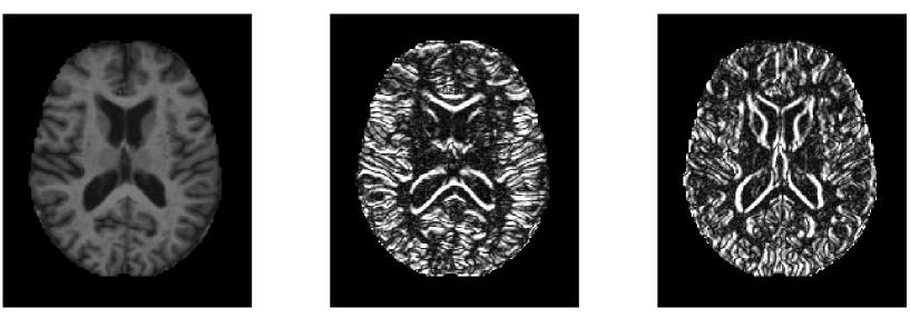
Figure 5: Original MRI image of person 144 and its derivatives in the horizontal and vertical direction.

The functional adjusted outlyingness of an MRI image $Y_{i}$ relative to the sample $\bm{Y}$ is given by (2) :

$$\text{fAO}(Y_{i};\bm{Y})=\frac{1}{176\times 208}\sum_{j=1}^{176}\sum_{k=1}^{208}\text{AO}(Y_{i}(j,k);\bm{Y}(j,k))\;,$$ (8)

where $\text{AO}(Y_{i}(j,k);\bm{Y}(j,k))$ is the adjusted outlyingness of the trivariate pixel $(j,k)$. The resulting FOM is presented in Figure 6.

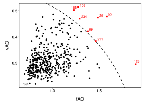
Figure 6: FOM of the MRI images dataset.

This plot indicates the presence of 8 outliers of several types. Image 126 has a remarkably high fAO combined with a relatively low vAO. This suggests a shift outlier, i.e. a function whose values are all shifted relative to the majority of the data. Images 29 and 92 have a large fAO in combination with a high vAO, indicating that they have strongly outlying subdomains. Images 108, 188 and 234 have an fAO which is on the high end relative to the dataset but which by itself does not make them outlying. Only in combination with their large vAO are they flagged as outliers. Images 69 and 211 have a CFO value just slightly above the cutoff, meaning they are borderline cases.

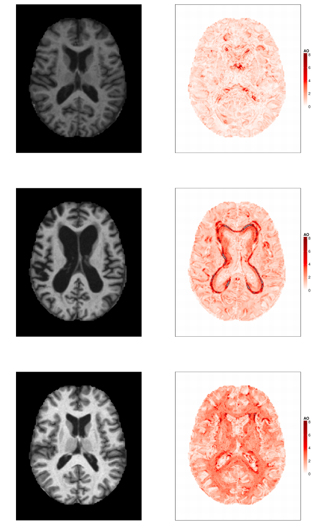
Figure 7: MRI image (left) and AO heatmap (right) of persons 144 (top), 92 (middle) and 126 (bottom).

A heatmap of the AO values can help to understand the root cause of an image’s outlyingness. In Figure 7 we compare the MRI images (left) and the AO maps (right) of persons 144, 92, and 126. (AO values of 8 or higher received the darkest color.) Image 144 has the smallest CFO value, and as such can be thought of as the least outlying image in the dataset. As expected, the AO heatmap of image 144 shows very few outlying pixels. For person 92, the AO heatmap nicely marks the region in which the MRI image deviates most from the majority of the images. Note that the boundaries of this region have the highest outlyingness. This is the result of including the derivatives in the analysis, as they emphasize the pixels at which the grayscale intensity changes. The AO heatmap of person 126 does not show any extremely outlying region but a rather high outlyingness over the whole domain, which explains its large fAO and regular vAO value. The actual MRI image to its left is globally lighter than the others, which confirms that it is a shift outlier.

5 Video data

This dataset consists of 633 images which together form a surveillance video of a beach, filmed with a static camera (Li et al.,, 2004). The data and the original video can be found at http://perception.i2r.a-star.edu.sg/bk_model/bk_index.html. The video first shows a beach with a tree during 8 seconds, shown in the leftmost frame of Figure 8. Then a man enters the screen from the left (second frame), disappears behind the tree (third frame), and then reappears again on the right side of the tree and stays on screen until the end of the video. The aim of applying our method to this dataset is to detect the man in this video. The images have $160\times 128$ pixels and are stored using the RGB (Red, Green and Blue) color model, so each image corresponds to three matrices, each of dimensions $160\times 128$. Overall we have 633 images $Y_{i}$ containing trivariate $Y_{i}(j,k)$ for $j=1,\ldots,J=160$ and $k=1,\ldots,K=128$.

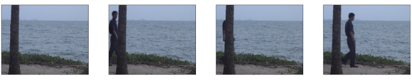
Figure 8: Frames number 100, 487, 491 and 500 from the video dataset.

Computing the fAO according to (2) yields the FOM in Figure 9. It is very instructive as the path of the man in the video can be traced in it. The first 480 images, which depict the beach and the tree and where only the water surface causes slight variations, are found on the bottom left side of the FOM inside the dashed curve that separates the regular frames from the outliers. Around frame 483 the man enters and as a result the standard deviation of the adjusted outlyingness rises slightly. The fAO itself increases more slowly as the fraction of the pixels covered by the man is still low. These frames can thus be classified as isolated outliers. Their CFO barely exceeds the cutoff (6) so on the FOM they are still close to the dashed line. Frames 484–487 have a very high fAO and vAO. In these images, the man is clearly visible between the left border of the frame and the tree. Consequently these images have outlying pixels in a substantial part of their domain. Frames 488–491 see the man disappear behind the tree. In these frames the fAO goes down as the fraction of outlying pixels decreases. From frame 492 onward the man reappears on the right side of the tree and stays in the screen until the end, as is reflected in the FOM since these frames contain many outlying pixels.

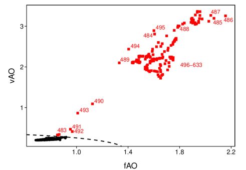
Figure 9: FOM of the video dataset.

In addition to the FOM we can construct AO heatmaps of individual frames. For frames 100, 487, 491 and 500, Figure 10 shows the raw image on the left, the AO heatmap in the middle and the FOM on the right. On the FOM we have drawn a blue circle around the relevant frame to indicate its location. This sequence of plots clearly shows that the proposed method works very well for this surveillance video data: not only can the man’s path be followed on the FOM, it is also clear from the AO heatmaps where exactly the man is in those frames. We have created a video in which the raw image, the AO heatmap and the FOM evolve over time alongside each other. It can be downloaded from http://wis.kuleuven.be/stat/robust/publ.

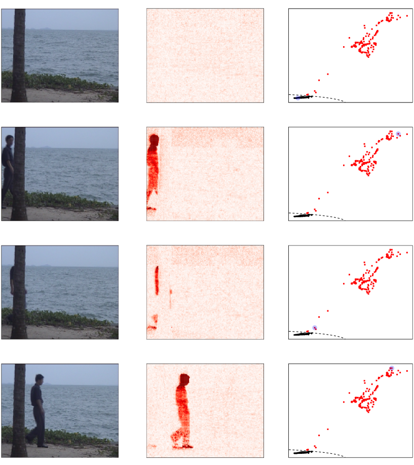
Figure 10: Frames 100, 487, 491 and 500 from the video dataset (left), the corresponding AO heatmaps (middle), and the FOM with marker on the position of the corresponding frame (right).

Appendix

The adjusted outlyingness of multivariate data has been introduced by Brys et al., (2005) and was studied in detail by Hubert and Van der Veeken, (2008). We first recall the adjusted outlyingness of a point $x$ relative to a univariate dataset $Y=\{y_{1},\ldots,y_{n}\}$. It can be seen as a robust version of the absolute $z$-score since it uses robust measures of location and scale (instead of the usual mean and standard deviation). It also accounts for skewness by computing the scale on each side of the median separately.

As a robust measure of location we take the median of $Y$. The robust estimates of scale are based on the adjusted boxplot (Hubert and Vandervieren,, 2008). This modified boxplot is well-suited for skewed distributions. First, an interval called the fence is computed. For right-skewed data it is given by

$$[Q_{1}(Y)-1.5\,e^{-4\text{MC}(Y)}\,\mbox{IQR}(Y)\;,\;Q_{3}(Y)+1.5\,e^{+3\text{MC}(Y)}\,\mbox{IQR}(Y)]$$

with $Q_{1}(Y)$ and $Q_{3}(Y)$ the first and third quartile of $Y$, $\mbox{IQR}(Y)=Q_{3}(Y)-Q_{1}(Y)$ and $\text{MC}(Y)$ the medcouple, a robust measure of skewness (Brys et al.,, 2004). For left-skewed data a similar definition holds. Note that for perfectly symmetric data the medcouple is zero, and then the fence is identical to that of the standard boxplot. The whiskers of the adjusted boxplot are lines from the box to the most remote data points inside the fence.

Figure 11 shows the adjusted boxplot of a right-skewed dataset $Y$. The points $x_{1}$ and $x_{2}$ have the same distance $d_{1}=d_{2}$ to the median of $Y$, but $x_{1}$ lies outside the lower whisker $w_{1}$ whereas $x_{2}$ lies inside the upper whisker. The adjusted outlyingness of $x_{1}<\mathop{\mbox{med}}(Y)$ is now defined as $d_{1}/s_{1}$ with $d_{1}=\mathop{\mbox{med}}(Y)-x_{1}$ and $s_{1}=\mathop{\mbox{med}}(Y)-w_{1}$. For $x_{2}>\mathop{\mbox{med}}(Y)$ the AO is given by $d_{2}/s_{2}$ with $d_{2}=x_{2}-\mathop{\mbox{med}}(Y)$ and $s_{2}=w_{2}-\mathop{\mbox{med}}(Y)$. In this example $\text{AO}(x_{1})>\text{AO}(x_{2})$.

Figure 11: Adjusted outlyingness based on the adjusted boxplot.

Formally, the univariate adjusted outlyingness AO of a point $x$ relative to a sample $Y$ is given by:

$$\mbox{AO}(x;Y)=\left\{\begin{array}[]{ll}\frac{x-\text{med}(Y)}{w_{2}(Y)-\text{med}(Y)}&\;\;\mbox{ if }x>\mathop{\mbox{med}}(Y)\\ \frac{\text{med}(Y)-x}{\text{med}(Y)-w_{1}(Y)}&\;\;\mbox{ if }x<\mathop{\mbox{med}}(Y)\;\;.\end{array}\right.$$ (9)

To compute the AO of a $p$-dimensional point $x$ relative to an $n\times p$ data matrix $Y$, the following projection pursuit procedure is applied. The point $x$ and all data points are projected on a direction $v$, and we compute the univariate AO of the projected point $x^{\prime}v$ relative to the projected dataset $Yv$ as in (9). This is repeated for many directions $v$, and the multivariate AO is defined as the maximum over all corresponding univariate AO’s:

$$\mbox{AO}(x;Y)=\sup_{||v||=1}\;\mbox{AO}(x^{\prime}v;Yv)\;\;.$$ (10)

This definition is based on the principle that a multivariate point is outlying with respect to a dataset if it is outlying in at least one direction of the multivariate space. Note that this outlying direction does not have to correspond to one of the coordinate axes.

To compute the multivariate AO we have to rely on approximate algorithms, as it is impossible to consider the projections on all directions $v$ in $p$-dimensional space. Hubert and Van der Veeken, (2008) suggest using $250p$ directions. A possible procedure to generate a direction is to randomly draw $p$ data points, compute the hyperplane passing through them, and then to take the direction orthogonal to it. This approach guarantees that the multivariate AO is affine invariant. This means that the AO does not change when we add a constant vector to the data, or multiply the data by a nonsingular $p\times p$ matrix.

References

- Brys et al., (2005) Brys, G., Hubert, M., and Rousseeuw, P. J. (2005). A robustification of Independent Component Analysis. Journal of Chemometrics, 19:364–375.
- Brys et al., (2004) Brys, G., Hubert, M., and Struyf, A. (2004). A robust measure of skewness. Journal of Computational and Graphical Statistics, 13:996–1017.
- Claeskens et al., (2014) Claeskens, G., Hubert, M., Slaets, L., and Vakili, K. (2014). Multivariate functional halfspace depth. Journal of the American Statistical Association, 109(505):411–423.
- Engelen et al., (2007) Engelen, S., Frosch Møller, S., and Hubert, M. (2007). Automatically identifying scatter in fluorescence data using robust techniques. Chemometrics and Intelligent Laboratory Systems, 86:35–51.
- Engelen and Hubert, (2011) Engelen, S. and Hubert, M. (2011). Detecting outlying samples in a parallel factor analysis model. Analytica Chimica Acta, 705:155–165.
- (6) Hubert, M., Rousseeuw, P. J., and Segaert, P. (2015a). Multivariate functional outlier detection. Statistical Methods & Applications, 24:177–202.
- (7) Hubert, M., Rousseeuw, P. J., and Segaert, P. (2015b). Rejoinder to ‘Multivariate functional outlier detection’. Statistical Methods & Applications, 24(2):269–277.
- Hubert and Van der Veeken, (2008) Hubert, M. and Van der Veeken, S. (2008). Outlier detection for skewed data. Journal of Chemometrics, 22:235–246.
- Hubert et al., (2012) Hubert, M., Van Kerckhoven, J., and Verdonck, T. (2012). Robust PARAFAC for incomplete data. Journal of Chemometrics, 26:290–298.
- Hubert and Vandervieren, (2008) Hubert, M. and Vandervieren, E. (2008). An adjusted boxplot for skewed distributions. Computational Statistics & Data Analysis, 52(12):5186–5201.
- Li et al., (2004) Li, L., Huang, W., Gu, I. Y.-H., and Tian, Q. (2004). Statistical modeling of complex backgrounds for foreground object detection. IEEE Transactions on Image Processing, 13:1459–1472.
- Marcus et al., (2007) Marcus, D., Wang, T., Parker, J., Csernansky, J., Morris, J., and Buckner, R. (2007). Open Access Series of Imaging Studies (OASIS): Cross-sectional MRI data in young, middle aged, nondemented, and demented older adults. Journal of Cognitive Neuroscience, 19:1498–1507.
- Saeys et al., (2008) Saeys, W., de Ketelaere, B., and Darius, P. (2008). Potential applications of functional data analysis in chemometrics. Journal of Chemometrics, 22:335–344.