Interference Management in Heterogeneous Networks with Blind Transmitters

Abstract

Future multi-tier communication networks will require enhanced network capacity and reduced overhead. In the absence of Channel State Information (CSI) at the transmitters, Blind Interference Alignment (BIA) and Topological Interference Management (TIM) can achieve optimal Degrees of Freedom (DoF), minimizing network’s overhead. In addition, Non-Orthogonal Multiple Access (NOMA) can increase the sum rate of the network, compared to orthogonal radio access techniques currently adopted by 4G networks. Our contribution is two interference management schemes, BIA and a hybrid TIM-NOMA scheme, employed in heterogeneous networks by applying user-pairing and Kornecker Product representation. BIA manages inter- and intra-cell interference by antenna selection and appropriate message scheduling. The hybrid scheme manages intra-cell interference based on NOMA and inter-cell interference based on TIM. We show that both schemes achieve at least double the rate of TDMA. The hybrid scheme always outperforms TDMA and BIA in terms of Degrees of Freedom (DoF). Comparing the two proposed schemes, BIA achieves more DoF than TDMA under certain restrictions, and provides better Bit-Error-Rate (BER) and sum rate perfomance to macrocell users, whereas the hybrid scheme improves the performance of femtocell users.

i Introduction

Over the past few years, cellular and wireless networks have been challenged by the increasing number of mobile Internet services and the constant growth of mobile data traffic. Future radio access networks should provide reduced latency, improved energy efficiency, and high user data rates in dense and high mobility network environments. The architecture of future communication networks will be heterogeneous in nature, i.e. macrocell with many small cells. The great challenge will be the employment of novel interference management strategies that will manage interference, without increasing the system’s overhead, and provide high data rates and reliable transmissions.

Interference Alignment (IA) was introduced by Maddah-Ali et al. in [1], and Jafar and Shamai in [4] for the MIMO X channels, and by Cadambe and Jafar in [7] for the $K$-user interference channel, where $K/2$ Degrees of Freedom (DoF) can be achieved. IA aligns the interfering signals present at each receiver into a low dimensional subspace, by linearly encoding signals in multiple dimensions, resulting in the desired signal being in a dimension unoccupied by interference links. Initially, IA required global Channel State Information (CSI) and was computationally complex.

Further work on IA led to the scheme of Blind IA, presented by Wang, Gou and Jafar in [10] and Jafar in [13], for certain network scenarios, which can achieve full DoF in the absence of CSI at the transmitters (CSIT), thus reducing the system overhead. Furthermore, Blind IA was introduced, by Jafar in [16], for cellular and heterogeneous networks, by “seeing” frequency reuse (i.e. orthogonal allocation of signaling dimensions) as a simple form of interference alignment. Blind IA in heterogeneous networks was generalized in [19] for the case of $K$ users in the macrocell and $K$ femtocells with one user each, introducing Kronecker (Tensor) Product representation and a variation of model parameters to optimize the sum rate performance. A special case of Blind IA, known as Topological Interference Management (TIM), was introduced by Jafar in [22]. TIM takes into consideration the position of every user in the cell(s), and based on their channel strength, weak interference links are ignored, resulting in $1/2$ DoF achieved for every user in the SISO Broadcast Channel (BC). In [25], Sun and Jafar research the scheme of TIM for the case of multiple receive and transmit antennas, concluding that only the former can provide more DoF in the network.

Unlike Orthogonal Frequency Division Multiple Access (OFDMA) and Single-Carrier Frequency Division Multiple Access (SC-FDMA) currently employed in 4G mobile networks, the scheme of Non-Orthogonal Multiple Access (NOMA), proposed in [28] by Saito et al., is based on a non-orthogonal approach to future radio access. According to NOMA, multiple users are superimposed in the power domain at the transmitters, and Successive Interference Cancellation (SIC) is performed at the receivers, improving capacity and throughput performance.

Power allocation and Quality-of-Service (QoS) for edge-cell users, has been a major issue to tackle in systems employing NOMA. It has been shown, in [31], that for the BC, if NOMA is employed with the aid of Coordinated Multiple Point (CoMP) and Alamouti Code, satisfactory rates for edge-cell users can be achieved without degrading the performance of users’ closer to the base station. Moreover, with an adaptive power and frequency resource allocation algorithm, as proposed in [34], targeting inter-cell interference, in order to boost the total throughput, reliable transmissions to edge-cell users can be obtained. Furthermore, in [37], authors study two different power allocation schemes, a fixed one and a cognitive radio inspired one, in a MIMO-NOMA model by using signal alignment and stochastic geometry.

Recently, research on NOMA has been focusing on user pairing to reduce complexity and improve efficiency. Cooperative NOMA schemes, where users with higher channel gains have prior information about other users’ messages, have been developed [40]. User pairing has been introduced in two NOMA schemes, discussed in [43], with one scheme employing fixed power allocation (F-NOMA) and another one inspired by cognitive radio (CR-NOMA), with users grouped differently in each one of the two NOMA schemes. In addition, user pairing has been studied in conjunction with the problem of power allocation, in [49], based on a new design of precoding and detection matrices. User pairing and the performance of NOMA have been also studied from an information theory perspective, as discussed in [46], researching the relationship between the rate region achieved by NOMA and the capacity region of the BC, observing that different power allocation to users corresponds to different points on the rate region graph, and showing that NOMA can outperform TDMA not only in terms of the sum rate, but for every users’s rate as well.

From the schemes of TIM and NOMA, a hybrid TIM-NOMA scheme emerged, introduced in [52] for the SISO BC and in [55] for the MIMO BC. The hybrid TIM-NOMA scheme divides users into groups, and manages “inter-group” interference based on the principles of TIM, and “intra-group” interference based on NOMA. The hybrid scheme can achieve double the sum rate of TDMA for high SNR values.

In this paper, based on [19, 52, 55], we introduce two interference management schemes employed in heterogeneous networks. For both schemes, we consider a $K$-user macrocell and $KL$ femtocells with one user each, taking into consideration the position of every user in the cell. The first scheme is a hybrid TIM-NOMA scheme based on [52, 55]. The novelty of this scheme is the fact that it changes the way user-grouping is performed compared to [52, 55]. Users in the macrocell belong to one group and then there exist $L$ groups of femtocells. Inter-cell interference is managed based on TIM and intra-cell interference based on NOMA. The second scheme is Blind IA in heterogeneous networks, which constitutes further work on [19]. Our contribution is the additional consideration of interference caused to femtocells by transmissions in the macrocell, and the existence of more than one femtocells around a macrocell user. The algorithms of both schemes are described by using Kronecker (Tensor) product representation. Based on our results, the hybrid scheme can achieve more total DoF compared to TDMA, whereas Blind IA outperforms TDMA in terms of DoF in most cases. We show that both schemes achieve higher sum rates than TDMA, as depicted in Figure 1. Finally, comparing the two schemes, Blind IA provides better sum-rate and BER performance to macrocell users, whereas the hybrid scheme results in better performance for the users in the femtocells, and based on its power allocation scheme provides QoS to edge cell users.

The rest of the paper is organized as follows. Section 2 describes the general network architecture, and the example-model which is used to describe the two schemes. Sections 3 and 4 present the model description and achievable sum rate of the hybrid and Blind IA schemes respectively. Section 5 describes the special case of Blind IA when $L=1$, i.e. only one femtocell interferes with every user in the macrocell. Section 6 discusses our results and the performance of the two schemes in terms of DoF, BER and sum rate. Finally, Section 7 summarizes the main findings of our work and discusses further developments.

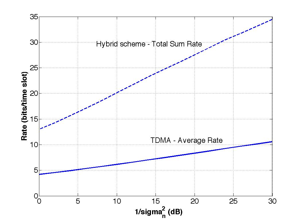
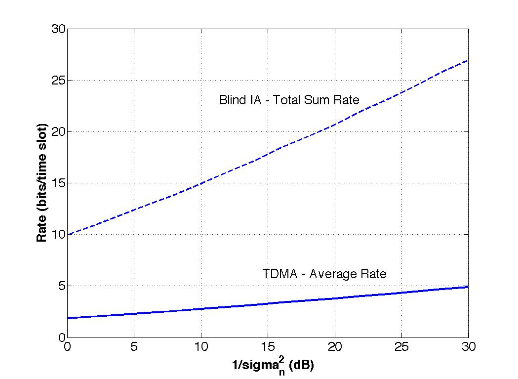
Figure 1: Sum Rate Performance: (left) Hybrid vs. TDMA, (right) Blind IA vs. TDMA. Both schemes achieve higher sum rates than TDMA

ii System Model

Consider the Broadcast Channel of a heterogeneous network, as shown in Figure 2, with 1 macrocell and $KL$ femtocells. At the $N\times N$ MIMO BC of the macrocell, there is one transmitter $T_{xA}$ with $N$ antennas, and $K$ users equipped with $N$ antennas each. Transmitter $T_{xA}$ has $N$ messages to send to every user, and when it transmits to user $a_{k}$, where $k\in\left\{1,2,...,K\right\}$, it causes interference to the other $K-1$ users in the macrocell and all the femtocell users $f_{kl}$. $L$ femtocells are considered to interfere with every macrocell user. At the $N\times N$ MIMO BC of each femtocell, there is one transmitter $T_{xkl}$ with $N$ antennas, and one user $f_{kl}$ equipped with $N$ antennas. When transmitter $T_{xkl}$ transmits to user $f_{kl}$, it causes interference to the macrocell user $a_{k}$ and to all or some (depending on the scheme we use) of the remaining $L-1$ neighbouring femtocell users $f_{kl}$. We consider that all channels remain constant over $T$ time slots (i.e. supersymbol) and we take into consideration the position of users in the cells, as summarized in Table I.

In the hybrid TIM-NOMA scheme, users are divided into $G=T=L+1$ groups. In the macrocell, all users belong to the same group $G_{0}$. In addition, there are $L$ different groups of femtocell users, with $G_{l}=\left\{f_{1l},f_{2l},...,f_{Kl}\right\}$ for $l\in\left\{1,2,...,L\right\}$. Moreover, $N$ messages are transmitted to every user in the femtocells.

In the Blind IA scheme, the number of neighbouring femtocells cannot be greater than 3, i.e. $L\leqslant 3$, with $L\leqslant N$. There is no grouping in the macrocell. Every macrocell user receives interference from $L$ femtocells. Thus, for all $k$, with $k\in\left\{1,2,...,K\right\}$, femtocell users are divided into two groups: Group $G_{1}$ consists of $(L-1)$ femtocell users $f_{kl}$, i.e. $G_{1}=\left\{f_{1l},f_{2l},...,f_{Kl}\right\}$, where $l\in\left\{1,...,L\right\}$ and $l\neq 2$. Group $G_{2}$ consists of femtocell users $f_{kl}$, i.e. $G_{2}=\left\{f_{1l},f_{2l},...,f_{Kl}\right\}$, where $l=2$. Femtocells in $G_{1}$ do not interfere with each other. Femtocells in $G_{2}$ interfere with all femtocells in $G_{1}$. In addition, $\mathcal{M}_{1}=\left(K-1\right)\left(N-\left(L-1\right)\right)$ messages are sent to users in $G_{1}$, and $\mathcal{M}_{2}=1$ messages are sent to users in $G_{2}$.

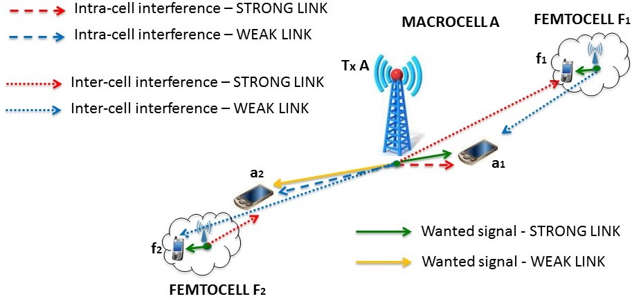
Figure 2: Heterogeneous network: $K=2$ users in macrocell and $KL=2$ femtocell ($L=1$) with 1 user each ($N=2$ transmit and receive antennas).

In this paper, we consider the following example model: In the macrocell, there are $K=2$ users, $N=2$ messages intended for every user, and $N=2$ transmit and receive antennas. Additionally there are $KL=2$ femtocells (note that $L=1$), with $N=2$ transmit and receive antennas each. For the hybrid scheme, we consider $N=2$ messages sent to every femtocell user, $T=2$ time slots and $G=2$ groups ($\left\{G_{0},G_{1}\right\}$), and for the Blind IA scheme, $\mathcal{M}_{1}=2$ messages sent to users in $G_{1}$, $T=3$ time slots and $G=1$ groups ($\left\{G_{1}\right\}$).

Description	Value
Macrocell Radius	$5\,km$
Femtocell Radius	$0.2\,km$
Reuse Distance Macrocell-Femtocell $F_{1}$	$5\,km$
Reuse Distance Macrocell-Femtocell $F_{2}$	$5.2\,km$
Distance of $a_{1}$ from $T_{x_{A}}$	$0.5\,km$
Distance of $a_{2}$ from $T_{x_{A}}$	$4.5\,km$
Distance of $f_{1}$ from $T_{x_{F1}}$	$0.2\,km$
Distance of $f_{2}$ from $T_{x_{F2}}$	$0.2\,km$

Table I: Distance metrics for the example model heterogeneous network.

iii Hybrid TIM-NOMA scheme

In the macrocell, the $TN\times 1$ signal at receiver $a_{k}$, considering slow fading (i.e. channels are fixed through transmission time), is given by:

$$\mathbf{y}_{a_{k}}=\mathbf{H}_{a_{k}}\mathbf{x}_{A}+\sum_{l=1}^{L}\mathbf{H}_{f_{kl}a_{k}}\mathbf{x}_{kl}+\mathbf{z}_{a_{k}},$$ (1)

where $\mathbf{H}_{a_{k}}\in\mathbb{C}^{(TN\times TN)}$ is the channel transfer matrix from $T_{x_{A}}$ to receiver $a_{k}$ and is given by $\mathbf{H}_{a_{k}}=\sqrt{\gamma_{a_{k}}}(\mathbf{I}_{T}\otimes\mathbf{h}_{a_{k}})$ (here and throughout $\mathbf{H}_{k}=\sqrt{\gamma_{k}}(\mathbf{I}_{T}\otimes\mathbf{h}_{k})$ with $\mathbf{h}_{k}$ denoting the channel coefficients from $T_{x_{K}}$ to $k$ for one time slot, $\gamma_{k}=1/d_{k}^{n}$ the path loss of user $k$ with $n$ denoting the path loss exponent considered for an urban environment ($n=3$), and $\otimes$ the Kronecker (Tensor) product). $\mathbf{H}_{f_{kl}a_{k}}\in\mathbb{C}^{(TN\times TN)}$ is the interference channel transfer matrix from $T_{x_{kl}}$ to receiver $a_{k}$ (here and throughout $\mathbf{H}_{xk}=\sqrt{\gamma_{xk}}(\mathbf{I}_{T}\otimes\mathbf{h}_{xk})$ with $\mathbf{h}_{xk}$ denoting the interference channel coefficients from $T_{x_{K}}$ to $k$ for one time slot). Due to the users’ different locations, channel coefficients are statistically independent, and follow an i.i.d. Gaussian distribution $\mathcal{CN}(0,1)$. Finally, $\mathbf{z}_{a_{k}}\sim\mathcal{CN}(0,\text{\leavevmode{sv}}_{n}^{2}\mathbf{I}_{TN})$ denotes the independent Additive White Gaussian Noise (AWGN) at the input of receiver $a_{k}$.

Taking into consideration the position of each user $a_{k}$ in the macrocell, users are ordered increasingly, in increasing order of path loss $\gamma_{a_{k}}$.

Example 1.

For the example model, assuming both macrocell users have the same received noise power $\text{\leavevmode{sv}}_{n}^{2}$, it follows:

$$\gamma_{1}>\gamma_{2},$$ (2)

with user 1 being very close to the base station and user $2$ at the edge of the cell. Weaker channels, of users’ being far from the base station, need to be boosted, such that for the transmit power $P_{k}$ of every user it holds that $P_{2}>P_{1}$. For every user $a_{k}$ in the macrocell, we choose to take their transmitted power, as initially suggested in [52], given by:

$$P_{a_{k}}=\frac{a^{2}}{N}\frac{d_{a_{k}}^{2}}{\sum_{j=1}^{K}d_{a_{j}}^{2}},$$ (3)

where $a\in\mathbb{R}$ is a constant determined by power considerations (see (4)). The total transmit power in the macrocell is given by the power constraint:

$$P_{macrocell}=\sum_{j=1}^{K}d_{a_{j}}^{2}P_{a_{j}}\mathrm{norm}(\mathbf{u}_{a_{j}})=a^{2}.$$ (4)

Then, the $T\times 1$ transmitted vector $\mathbf{x}_{A}$ is given by:

$$\mathbf{x}_{A}=\left(\mathbf{v}_{0}\otimes\mathbf{I}_{N}\right)\sum_{k=1}^{K}\sqrt{P_{a_{k}}}\mathbf{u}_{a_{k}},$$ (5)

with $\mathbf{v}_{0}$ denoting the $T\times 1$ precoding vector corresponding to group $G_{0}$ that macrocell users belong to, and should be orthogonal to all the remaining $T-1$ precoding vectors (corresponding to $T-1$ groups).

In each femtocell, the $TN\times 1$ signal at receiver $f_{kl}$ is given by:

$$\mathbf{y}_{f_{kl}}=\mathbf{H}_{f_{kl}}\mathbf{x}_{f_{kl}}+\mathbf{H}_{Af_{kl}}\mathbf{x}_{A}+\sum_{\overset{j=1}{j\neq l}}^{L}\mathbf{H}_{f_{kj}f_{kl}}\mathbf{x}_{kj}+\mathbf{z}_{f_{kl}},$$ (6)

where $\mathbf{H}_{f_{kl}}\in\mathbb{C}^{(TN\times TN)}$ is the channel transfer matrix from $T_{xkl}$ to receiver $f_{kl}$, $\mathbf{H}_{Af_{kl}}\in\mathbb{C}^{(TN\times TN)}$ is the channel transfer matrix from $T_{x_{A}}$ to receiver $f_{kl}$, and $\mathbf{H}_{f_{kj}f_{kl}}\in\mathbb{C}^{(TN\times TN)}$ is the channel transfer matrix from $T_{xkj}$ to receiver $f_{kl}$. Finally, $\mathbf{z}_{f_{kl}}\sim\mathcal{CN}(0,\text{\leavevmode{sv}}_{n}^{2}\mathbf{I}_{TN})$ denotes the independent AWGN at the input of receiver $f_{kl}$.

For user $f_{kl}$ in every femtocell, their transmitted power is given by $P_{f_{kl}}=b^{2}/N$, where $b\in\mathbb{R}$ is a constant determined by power considerations (see (7)), and the total transmit power in the femtocell is given by:

$$P_{f_{emtocell}}=b^{2}.$$ (7)

Then, the $T\times 1$ transmitted vector $\mathbf{x}_{f_{kl}}$ is given by:

$$\mathbf{x}_{f_{kl}}=\left(\mathbf{v}_{l}\otimes\mathbf{I}_{N}\right)\sqrt{P_{f_{kl}}}\mathbf{u}_{f_{kl}},$$ (8)

with $\mathbf{v}_{l}$ denoting the $T\times 1$ precoding unit vector corresponding to group $G_{l}$ that user $f_{kl}$ belongs to, and should be orthonormal to all the remaining $T-1$ precoding vectors.

Example 2.

For the example model, we choose the precoding vectors $\mathbf{v}_{0}$ and $\mathbf{v}_{1}$, for groups $G_{0}$ and $G_{1}$ respectively, as $\mathbf{v}_{0}=\begin{bmatrix}1/2&\sqrt{3}/2\end{bmatrix}^{T}$,$\mathbf{v}_{1}=\begin{bmatrix}-\sqrt{3}/2&1/2\end{bmatrix}^{T}$, where $G_{0}=\left\{a_{1},a_{2}\right\}$ and $G_{1}=\left\{f_{\text{11}},f_{21}\right\}$.

iii-A Inter-cell Interference Management

In the network, there will be one $T\times 1$ unit precoding vector $\mathbf{v}_{0}$ for the macrocell and ($T-1$) $T\times 1$ unit precoding vectors $\mathbf{v}_{l}$, where $l\in\left\{1,2,...,L\right\}$, for the femtocells, with all precoding vectors being orthogonal to each other.

Theorem 3.

In the macrocell, multiplying the received signal $\mathbf{y}_{a_{k}}$ with $\mathbf{v}_{0}{}^{T}\otimes\mathbf{I}_{N}$, the resulting signal at every receiver $a_{k}$, is given by:

$$\widetilde{\mathbf{y}}_{a_{k}}=\left(\sum_{j=1}^{K}\sqrt{P_{a_{j}}}\sqrt{\gamma_{a_{k}}}\mathbf{h}_{a_{k}}\mathbf{u}_{a_{j}}\right)+\widetilde{\mathbf{z}_{a_{k}}},$$ (9)

where $\widetilde{\mathbf{z}_{a_{k}}}=\left(\mathbf{v}_{0}{}^{T}\otimes\mathbf{I}_{N}\right)\mathbf{z}_{a_{k}}$ remains white noise with the same variance.

Proof:

We show that $\left(\mathbf{v}_{0}{}^{T}\otimes\mathbf{I}_{N}\right)$ removes inter-cell interference at the $k$th receiver $a_{k}$:

$$\left(\mathbf{v}_{0}^{T}\otimes\mathbf{I}_{N}\right)\mathbf{y}_{a_{k}} =\left(\mathbf{v}_{0}^{T}\otimes\mathbf{I}_{N}\right)\left(\sqrt{\gamma_{a_{k}}}(\mathbf{I}_{T}\otimes\mathbf{h}_{a_{k}})\left(\mathbf{v}_{0}\otimes\mathbf{I}_{N}\right)\sum_{k=1}^{K}\sqrt{P_{a_{k}}}\mathbf{u}_{a_{k}}\right)$$

$$+\left(\mathbf{v}_{0}^{T}\otimes\mathbf{I}_{N}\right)\left(\sum_{l=1}^{L}\sqrt{\gamma_{f_{kl}a_{k}}}(\mathbf{I}_{T}\otimes\mathbf{h}_{f_{kl}a_{k}})\left(\mathbf{v}_{l}\otimes\mathbf{I}_{N}\right)\sqrt{P_{f_{kl}}}\mathbf{u}_{f_{kl}}\right)+\widetilde{\mathbf{z}_{a_{k}}}$$

$$=\sum_{j=1}^{K}\sqrt{P_{a_{j}}}\sqrt{\gamma_{a_{k}}}\mathbf{h}_{a_{k}}\mathbf{u}_{a_{j}}+\sum_{l=1}^{L}\sqrt{\gamma_{f_{kl}a_{k}}}\left(\mathbf{v}_{0}^{T}\mathbf{v}_{l}\otimes\mathbf{h}_{f_{kl}a_{k}}\right)\sqrt{P_{f_{kl}}}\mathbf{u}_{f_{kl}}+\widetilde{\mathbf{z}_{a_{k}}},$$ (10)

where by definition, for $l=1,\ldots,L$, $\mathbf{v}_{0}{}^{T}\mathbf{v}_{l}=0$. ∎

Theorem 4.

In the femtocell, multiplying the received signal $\mathbf{y}_{f_{kl}}$ with $\mathbf{v}_{l}{}^{T}\otimes\mathbf{I}_{N}$, the resulting signal at every receiver $f_{kl}$, is given by:

$$\widetilde{\mathbf{y}}_{f_{kl}}=\sqrt{\gamma_{f_{kl}}}\sqrt{P_{f_{kl}}}\mathbf{h}_{f_{kl}}\mathbf{u}_{f_{kl}}+\widetilde{\mathbf{z}_{f_{kl}}},$$ (11)

where $\widetilde{\mathbf{z}_{f_{kl}}}=\left(\mathbf{v}_{l}{}^{T}\otimes\mathbf{I}_{N}\right)\mathbf{z}_{f_{kl}}$ remains white noise with the same variance.

Proof:

We show that $\left(\mathbf{v}_{l}{}^{T}\otimes\mathbf{I}_{N}\right)$ removes inter-cell interference at the $kl$th receiver $f_{kl}$:

$$\left(\mathbf{v}_{l}^{T}\otimes\mathbf{I}_{N}\right)\mathbf{y}_{f_{kl}} =\sqrt{\gamma_{f_{kl}}}\sqrt{P_{f_{kl}}}\mathbf{h}_{f_{kl}}\mathbf{u}_{f_{kl}}+\sqrt{\gamma_{Af_{kl}}}\left(\mathbf{v}_{l}{}^{T}\mathbf{v}_{0}\otimes\mathbf{h}_{Af_{kl}}\right)\sum_{j=1}^{K}\sqrt{P_{a_{j}}}\mathbf{u}_{a_{j}}$$

$$+\sum_{\overset{j=1}{j\neq l}}^{L}\sqrt{\gamma_{f_{kj}f_{kl}}}\left(\mathbf{v}_{l}^{T}\mathbf{v}_{j}\otimes\mathbf{h}_{f_{kj}f_{kl}}\right)\sqrt{P_{f_{kj}}}\mathbf{u}_{f_{kj}}+\widetilde{\mathbf{z}_{f_{kl}}},$$ (12)

where by definition, for $l=1,\ldots,L$, $\mathbf{v}_{0}{}^{T}\mathbf{v}_{l}=0$, and for $j=1,\ldots,L$ and $j\neq l$, $\mathbf{v}_{l}{}^{T}\mathbf{v}_{j}=0$.∎

Example 5.

For the example model, for groups $G_{0}$ and $G_{1}$, the post-processed signals at receivers $a_{1}$ and $f_{1}$ are:

$$\widetilde{\mathbf{y}_{a_{1}}}=\sum_{j=1}^{2}\sqrt{P_{a_{j}}}\sqrt{\gamma_{a_{1}}}\mathbf{h}_{a_{1}}\mathbf{u}_{a_{j}}+\widetilde{\mathbf{z}_{a_{1}}},$$

$$\widetilde{\mathbf{y}_{f_{1}}}=\sqrt{\gamma_{f_{1}}}\sqrt{P_{f_{1}}}\mathbf{h}_{f_{1}}\mathbf{u}_{f_{1}}+\widetilde{\mathbf{z}_{f_{1}}}.$$

iii-B Intra-cell Interference Management

The concept of NOMA will be only applied to group $G_{0}$ since only users in the macrocell experience intra-cell interference. Users are ordered in increasing order of their path loss $\gamma_{a_{k}}$ and SIC is performed at every receiver. Each user $a_{k}$ can correctly decode the signals of users whose path loss is smaller than theirs by considering their own signal as noise. In the case that $a_{k}$ receives interference from transmissions to users in the macrocell that have a larger path loss than they do, then $a_{k}$ decodes their own signal considering interference as noise. Maximum Likelihood (ML) reception is performed every time a user decodes its own or another user’s signal.

Example 6.

The decoding order for the macrocell users is given in (2). Receiver $a_{2}$ decodes their own signal, considering interference from transmissions to user $a_{1}$ as noise. Receiver $a_{1}$ decodes first signal $\mathbf{u}_{a_{2}}$ (finding $\widetilde{\mathbf{u}_{a_{2}}}$), considering their own signal as noise, and subtracts the estimate $\widetilde{\mathbf{u}_{a_{2}}}$ from their post-processed signal $\widetilde{\mathbf{y}_{a_{1}}}$. Then, they decode their own signal as $\widetilde{\widetilde{\mathbf{y}_{a_{1}}}}=\widetilde{\mathbf{y}_{a_{1}}}-\sqrt{\gamma_{a_{1}}}\sqrt{P_{a_{1}}}\mathbf{h}_{a_{1}}\widetilde{\mathbf{u}_{a_{2}}}$, which if $\widetilde{\mathbf{u}_{a_{2}}}=\mathbf{u}_{a_{2}}$ reduces to the interference-free channel.

iii-C Achievable Sum Rate

In the macrocell, the total rate for each user $a_{k}$ per time slot, setting $S=\left({\displaystyle\sum_{\overset{j\in G_{0}}{j<k}}}\left|\mathbf{h}_{a_{k}}\right|^{2}P_{a_{j}}+\sigma_{n}^{2}\right)$, is given by:

$$R_{a_{k}}=\frac{1}{T}\mathbb{E}\left[\log\det\left(\mathbf{I}_{N}+\frac{P_{macrocell}}{NS}\frac{d_{a_{k}}^{2}}{{\displaystyle\sum_{j=1}^{K}}d_{a_{j}}^{2}}\gamma_{a_{k}}\mathbf{h}_{a_{k}}\mathbf{h}_{a_{k}}^{T}\right)\right],$$ (13)

where $a_{k}\in G_{0}$.

In every femtocell, the total rate for each user $f_{kl}$, per time slot is given by:

$$R_{f_{kl}}=\frac{1}{T}\mathbb{E}\left[\log\det\left(\mathbf{I}_{N}+\frac{P_{femtocell}}{N\sigma_{n}^{2}}\gamma_{f_{kl}}\mathbf{h}_{f_{kl}}\mathbf{h}_{f_{kl}}^{T}\right),\right]$$ (14)

where $f_{kl}\in G_{l}$.

iv Blind Interference Alignment

In the macrocell, The $NT\times 1$ signal at receiver $a_{k}$, for the supersymbol, is given by (1).

The total transmit power, as initially presented in [19], is given by the power constraint:

$$P_{\mathrm{macrocell}}=\mathbb{E}[\mathrm{tr}(\mathbf{x}_{A}\mathbf{x}_{A}^{T})]=KNa^{2}.$$ (15)

Then, the $NT\times 1$ transmitted vector $\mathbf{x}_{A}$ is given by:

$$\mathbf{x}_{A}=\sum_{i=1}^{K}\mathbf{V}^{[a_{i}]}\mathbf{u}^{[a_{i}]},$$ (16)

where $\mathbf{u}^{[a_{k}]}$ is the $N\times 1$ data stream vector of each user $a_{k}$, and $\mathbf{V}^{[a_{k}]}$ is the $NT\times N$ beamforming matrix of user $a_{k}$. As mentioned in [19], the choice of the $NT\times N$ beamforming matrices $\mathbf{V}^{[a_{k}]}$ carrying messages to users in the macrocell is not unique and should lie in a space that is orthogonal to the channels of the other $K-1$ macrocell users. The beamforming matrix for user $a_{k}$ is given by ([19], (2)):

$$\mathbf{V}^{[a_{k}]}=\frac{a}{\sqrt{N}}(\mathbf{v}^{[a_{k}]}\otimes\mathbf{I}_{N}),$$ (17)

where $a\in\mathrm{\mathfrak{\boldsymbol{\mathfrak{\mathcal{\mathbb{R}}}}}}$ is a constant determined by power considerations (see (15)), and $T\times 1$ $\mathbf{v}^{[a_{k}]}$ should be a unit vector with entries equal to $c$, $\sqrt{1-c^{2}}$ (for $c\in\mathrm{\mathfrak{\boldsymbol{\mathfrak{\mathcal{\mathbb{R}}}}}}$ and $c\neq 0,\pm 1$) or $0$, with a different combination for every $a_{k}$. For every macrocell user, there will be one time slot in which only they will be receiving messages. Also, there will be another time slot (time slot 1 in Figure 2) over which $T_{xA}$ will transmit to all users.

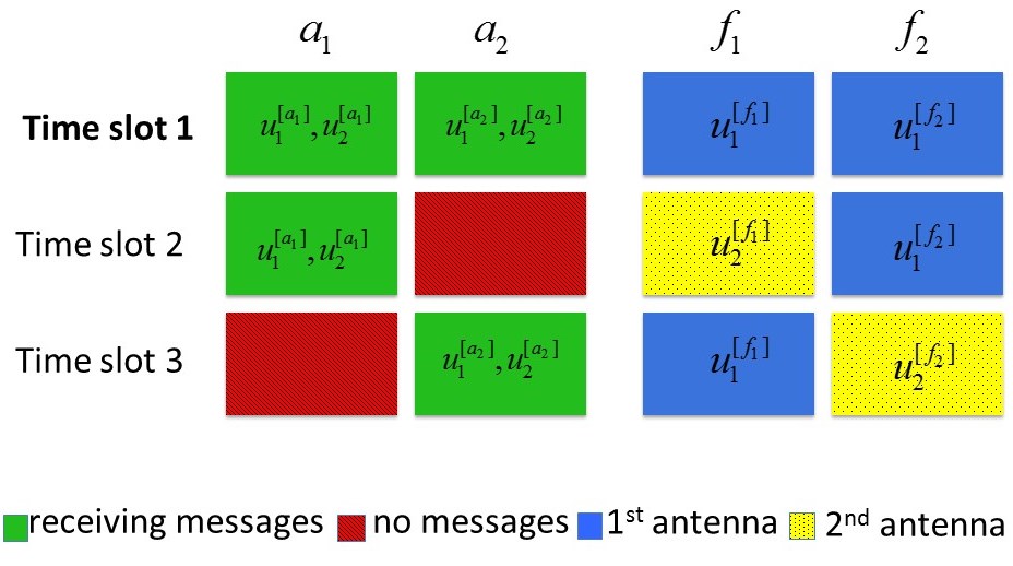
Figure 3: Beamforming in the macrocell and femtocells.

Example 7.

The beamforming matrices, as shown in Figure 2, are given by:

$$\mathbf{V}^{[a_{1}]}=\frac{a}{\sqrt{N}}(\mathbf{v}^{[a_{1}]}\otimes\mathbf{I}_{2})=\frac{a}{\sqrt{2}}\left(\begin{bmatrix}c&\sqrt{1-c^{2}}&0\end{bmatrix}^{T}\otimes\mathbf{I}_{2}\right),$$

$$\mathbf{V}^{[a_{2}]}=\frac{a}{\sqrt{N}}(\mathbf{v}^{[a_{2}]}\otimes\mathbf{I}_{2})=\left(\frac{a}{\sqrt{2}}\begin{bmatrix}c&0&\sqrt{1-c^{2}}\end{bmatrix}^{T}\otimes\mathbf{I}_{2}\right).$$

At each femtocell, for Group $G_{1}$, the $NT\times 1$ signal at receiver $f_{kl}$, for the supersymbol, is given by:

$$\mathbf{y}_{f_{kl}}=\mathbf{H}_{f_{kl}}\mathbf{x}{}_{f_{kl}}+\mathbf{H}_{Af_{kl}}\mathbf{x}_{A}+\mathbf{H}_{f_{k2}f_{kl}}\mathbf{x}_{f_{k2}}+\mathbf{Z}f_{kl},$$ (18)

and for Group $G_{2}$, the $NT\times 1$ signal at receiver $f_{k2}$, for the supersymbol, is given by:

$$\mathbf{y}_{f_{k2}}=\mathbf{H}_{f_{k2}}\mathbf{x}{}_{f_{k2}}+\mathbf{H}_{Af_{k2}}\mathbf{x}_{A}+{\displaystyle\sum_{\underset{l\neq 2}{l=1,...,L}}}\mathbf{H}_{f_{kl}f_{k2}}\mathbf{x}_{f_{kl}}+\mathbf{Z}_{f_{k2}}.$$ (19)

For Group $G_{1}$, the total transmit power is given by the power constraint:

$$P_{femtocell_{1}}=\mathcal{M}_{1}\frac{b_{1}^{2}}{N},$$ (20)

and the $NT\times 1$ vector, transmitted by $T_{x_{fl}}$ is given by:

$$\mathbf{x}{}_{f_{kl}}=\mathbf{V}^{[f_{kl}]}\mathbf{U}^{[f_{kl}]},$$ (21)

where $\mathbf{U}^{[f_{kl}]}$ is the $\mathcal{M}_{1}\times 1$ data stream vector of each user $f_{kl}$, and $\mathbf{V}^{[f_{kl}]}$ the $NT\times\mathcal{M}_{1}$ beamforming matrix given by:

$$\mathbf{V}^{[f_{kl}]}=\frac{b_{1}}{\sqrt{N}}\left(\sum_{i=1}^{T-1}\left(\mathbf{\xi}_{i}^{[f_{kl}]^{T}}\otimes\left(\mathbf{r}\mathbf{q}_{i}^{[f_{kl}]}\right)\right)\right),$$ (22)

where $b_{1}\in\mathrm{\mathfrak{\boldsymbol{\mathfrak{\mathcal{\mathbb{R}}}}}}$ is a constant determined by power considerations (see (20)), and $\mathbf{v}^{[f_{kl}]}=\sum_{i=1}^{T-1}\mathbf{\xi}_{i}^{[f_{kl}]}$ is an $1\times T$ vector, and for $i=1,...,T-1$, $\mathbf{\xi}_{i}^{[f_{kl}]}$ has one entry equal to $d$ or $\sqrt{1-(T-2)(N-(L-1))d^{2}}$ (for $d\in\mathrm{\mathfrak{\boldsymbol{\mathfrak{\mathcal{\mathbb{R}}}}}}$ and $d\neq 0,\pm\sqrt{\frac{1}{(T-2)(N-L+1)}}$), and the rest of its entries equal to $0$, such that $\mathbf{v}^{[f_{kl}]}=\sum_{i=1}^{T-1}\mathbf{\xi}_{i}^{[f_{kl}]}$ has one entry equal to $0$, one entry equal to $\sqrt{1-(T-2)d^{2}}$, and the rest of its entries equal to $d$. Moreover, we set $\mathbf{r}$ equal to the first $(N-L+1)$ columns of $\mathbf{I}_{N}$ with $\mathbf{e}_{1}$ equal to the sum of the first $(N-1)$ columns of $\mathbf{I}_{N}$. Furthermore, for $i\neq t_{1}$ ($t_{1}$ denoting the time slot that $T_{xA}$ broadcasts to all users in the macrocell), $\mathbf{q}_{i}^{[f_{kl}]}$ is equal to the submatrix of $\mathbf{I}_{\mathcal{M}_{1}}$ consisting of rows $((N-2)(i-1)+1,(N-2)i),$ and for $i=t_{1}$ $\mathbf{q}_{i}^{[f_{kl}]}$ is equal to any one of $\mathbf{q}_{i}^{[f_{kl}]}$ for $i\neq t_{1}$. The $t$th component of $\mathbf{\xi}_{i}^{[f_{k}]}$ being 1 means that in the $kl$th femtocell, the antennas determined by $\mathbf{r}$ are in use at time $t$ and the messages determined by $\mathbf{q}_{i}^{[f_{kl}]}$ are transmitted.

For Group $G_{2}$, the total transmit power is given by the power constraint:

$$P_{femtocell_{2}}=\mathcal{M}_{2}\frac{b_{2}^{2}}{N},$$ (23)

and the $NT\times\mathcal{M}_{2}$ beamforming matrix $\mathbf{V}^{[f_{kl}]}$ is given by:

$$\mathbf{V}^{[f_{kl}]}=\frac{b_{2}}{\sqrt{N}}\left(\mathbf{v}^{[f_{kl}]^{T}}\otimes\mathbf{e}_{2}\right),$$ (24)

where $b_{2}\in\mathrm{\mathfrak{\boldsymbol{\mathfrak{\mathcal{\mathbb{R}}}}}}$ is a constant determined by power considerations (see (23)), and $\mathbf{v}^{[f_{kl}]}$ is an $1\times T$ unit vector with its $t_{2}$th entry ($t_{2}$ denoting the time slot that $a_{k}$ receives no interference) equal to 1 and the rest of its entries equal to 0. Vector $\mathbf{e}_{2}$ is equal to the last column of $\mathbf{I}_{N}$.

iv-A Interference Management

In the macrocell, in order remove inter- and intra-cell interference, the received signal should be projected to a subspace orthogonal to the subspace that interference lies in.

Definition 8.

The rows of the $N\times NT$ projection matrix $\mathbf{P}^{[a_{k}]}={\displaystyle\sum_{s=1}^{2}}\left(\mathbf{w}_{s}^{[a_{k}]}\otimes\left(\mathbf{D}_{s}^{[a_{k}]}\widetilde{\mathbf{h}}^{[f_{k}a_{k}]}\right)\right)$, form an orthonormal basis of this subspace, where

1. for all s, the $1\times T$ $\mathbf{w}_{s}^{[a_{k}]}$ is a unit vector orthogonal to $\mathbf{v}^{[a_{i}]}$ for $i\neq k$,

2. $\mathbf{w}_{s}^{[a_{k}]}$ has coefficients equal to zero on the non-zero values of $\mathbf{\xi}_{i}^{[f_{kl}]^{T}}$ for $i=1,2,...,T-1$, $s=2$, $l=1,...,L$ and $l\neq 2$, and $\mathbf{\mathbf{v}}^{[f_{kl}]^{T}}$for $s=1$ and $l=2$,

3. $\mathbf{D}_{1}^{[a_{k}]}=\mathrm{diag}(\mathbf{e}_{2})$ and $\mathbf{D}_{2}^{[a_{k}]}=\mathrm{diag}(\mathbf{e}_{1})$,

4. $\mathbf{\widetilde{h}}^{[f_{k}a_{k}]}$ is an $N\times N$ matrix, whose rows are unit vectors, with the $N$th row orthogonal to all the columns of $\left(\mathbf{h}^{[f_{kl}a_{k}]}\mathbf{r}\right)$ for all $l=1,...,L$ and $l\neq 2$, and the remaining $(N-1)$ rows orthogonal to the columns $\left(\mathbf{h}^{[f_{kl}a_{k}]}\mathbf{\mathbf{e}}_{2}\right)$ for $l=2$.

Theorem 9.

Multiplying the received signal by projection matrix $\mathbf{P}^{[a_{k}]}$:

$$\mathbf{\widetilde{y}}^{[a_{k}]}=\mathcal{\mathbf{P}}^{[a_{k}]}\mathbf{y}^{[a_{k}]}=\mathcal{\mathbf{\mathcal{H}}}^{[a_{k}]}\mathbf{U}^{[a_{k}]}+\mathbf{\widetilde{Z}}^{[a_{k}]},$$ (25)

where

$$\mathcal{\mathbf{\mathcal{H}}}^{[a_{k}]}=\frac{a}{\sqrt{N}}\mathcal{D}^{[a_{k}]}\mathcal{K}^{[a_{k}]},$$ (26)

with diagonal matrix

$$\mathcal{D}^{[a_{k}]}={\displaystyle\sum_{s=1}^{2}}\mathbf{w}_{s}^{[a_{k}]}\mathbf{v}^{[a_{k}]}\mathbf{D}_{s}^{[a_{k}]}=\mathrm{diag}\left(\mathbf{w}_{s}^{[a_{k}]}\mathbf{v}^{[a_{k}]}\right),$$ (27)

and

$$\mathcal{K}^{[a_{k}]}=\sqrt{\gamma_{a_{k}}}\mathbf{\widetilde{h}}^{[f_{k}a_{k}]}\mathbf{h}^{[a_{k}]},$$ (28)

and $\mathbf{\widetilde{Z}}^{[a_{k}]}=\mathcal{\mathbf{P}}^{[a_{k}]}\mathbf{Z}^{[a_{k}]}$ remains white noise with the same variance (since $\mathbf{w}_{s}^{[a_{k}]}$ is a unit vector).

In the femtocells and for Group $G_{1}$, in order remove inter- and intra-cell interference, the received signal should be projected to a subspace orthogonal to the subspace that interference lies in.

Definition 10.

For Group $G_{1}$, the rows of the $\mathcal{M}_{1}\times NT$ projection matrix $\mathbf{P}^{[f_{kl}]}=\mathbf{w}\otimes\mathbf{W}^{[f_{kl}]}$ , form an orthonormal basis of this subspace, where

1. the $1\times T$ $\mathbf{w}$ is a unit vector orthogonal to $\mathbf{v}^{[a_{i}]}$ for all $i$,

2. and $\mathbf{W}^{[f_{kl}]}$ is an $\mathcal{M}_{1}\times N$ matrix whose rows are orthogonal to the columns of $\left(\mathbf{h}^{[f_{k2}f_{kl}]}\mathbf{e}_{2}\right)$.

Theorem 11.

Multiplying the received signal by projection matrix $\mathbf{P}^{[f_{kl}]}$:

$$\mathbf{\widetilde{y}}^{[f_{kl}]}=\mathcal{\mathbf{P}}^{[f_{kl}]}\mathbf{y}^{[f_{kl}]}=\mathcal{\mathbf{\mathcal{H}}}^{[f_{kl}]}\mathbf{U}^{[f_{kl}]}+\mathbf{\widetilde{Z}}^{[f_{kl}]},$$ (29)

where the $\mathcal{M}_{1}\times\mathcal{M}_{1}$ effective channel matrix is given by:

$$\mathcal{\mathbf{\mathcal{H}}}^{[f_{kl}]}=\frac{b_{1}}{\sqrt{N}}\mathcal{K}^{[f_{kl}]}\mathcal{D}^{[f_{kl}]},$$ (30)

where

$$\mathcal{K}^{[f_{kl}]}=\sqrt{\gamma_{f_{kl}}}\mathbf{W}^{[f_{kl}]}\mathbf{h}^{[f_{kl}]}\mathbf{r},\;\mathcal{D}^{[f_{kl}]}={\displaystyle\sum_{s=1}^{T-1}}\mathbf{w}\xi_{i}^{[f_{kl}]^{T}}\mathbf{q}_{i}^{[f_{kl}]},$$ (31)

and $\mathbf{\widetilde{Z}}^{[f_{kl}]}=\mathcal{\mathbf{P}}^{[f_{kl}]}\mathbf{Z}^{[f_{kl}]}$ remains white noise with the same variance (since $\mathbf{w}$ is a unit vector).

Definition 12.

For Group $G_{2}$, the rows of the $\mathcal{M}_{2}\times NT$ projection matrix $\mathbf{P}^{[f_{kl}]}=\mathbf{w}\otimes\mathbf{W}^{[f_{kl}]},$ , form an orthonormal basis of this subspace, where

1. the $1\times T$ $\mathbf{w}$ is a unit vector orthogonal to $\mathbf{v}^{[a_{i}]}$ for all $i$,

2. and $\mathbf{W}^{[f_{kl}]}$ is an $\mathcal{M}_{2}\times N$ vector orthogonal to the columns of $\left(\mathbf{h}^{[f_{kl}f_{k2}]}\mathbf{r}\right)$ for $l=1,...,L$ and $l\neq 2$.

Theorem 13.

Multiplying the received signal by projection matrix $\mathbf{P}^{[f_{kl}]}$:

$$\mathbf{\widetilde{y}}^{[f_{kl}]}=\mathcal{\mathbf{P}}^{[f_{kl}]}\mathbf{y}^{[f_{kl}]}=\mathcal{\mathbf{\mathcal{H}}}^{[f_{kl}]}\mathbf{U}^{[f_{kl}]}+\mathbf{\widetilde{Z}}^{[f_{kl}]},,$$ (32)

where the $\mathcal{M}_{2}\times\mathcal{M}_{2}$ effective channel matrix (actually a number), is given by:

$$\mathcal{\mathbf{\mathcal{H}}}^{[f_{kl}]}=\frac{b_{B}}{\sqrt{N}}\mathcal{\delta}^{[f_{kl}]}\mathcal{K}^{[f_{kl}]},$$ (33)

where

$$\mathcal{\delta}^{[f_{kl}]}=\mathbf{w}\mathbf{v}^{[f_{kl}]^{T}},\;\mathcal{K}^{[f_{kl}]}=\sqrt{\gamma_{f_{kl}}}\mathbf{W}^{[f_{kl}]}\mathbf{h}^{[f_{kl}]}\mathbf{e}_{2}$$ (34)

and $\mathbf{\widetilde{Z}}^{[f_{kl}]}=\mathcal{\mathbf{P}}^{[f_{kl}]}\mathbf{Z}^{[f_{kl}]}$ remains white noise with the same variance (since $\mathbf{w}$ is a unit vector).

iv-B Achievable Sum Rate

In the macrocell, since there is no CSIT, the total rate for each user for ONE time slot, is given by:

$$R^{[a_{k}]}=\frac{1}{T}\mathrm{\mathtt{\mathbb{E}}}\left[\log\det\left(\mathbf{I}_{N}+\frac{P_{\mathrm{macrocell}}}{KN^{2}\sigma_{n}^{2}}\mathcal{D}^{[a_{k}]}\mathcal{K}^{[a_{k}]}\mathcal{K}^{[a_{k}]^{*}}\mathcal{D}^{[a_{k}]^{*}}\right)\right].$$ (35)

For any channel realization, in the high SNR limit, the rate is maximized by maximizing the value of

$$\mathrm{det}\mathcal{D}^{[a_{k}]}=\prod_{s=1}^{2}\left(\mathbf{w}_{s}^{[a_{k}]}\mathbf{v}^{[a_{k}]^{T}}\right).$$ (36)

For Group $G_{1}$, in each femtocell, since there is no CSIT, the rate for each user, for ONE time slot, is given by:

$$R^{[f_{kl}]}=\frac{1}{T}\mathcal{\mathbb{E}}\left[\log\det\left(\mathbf{I}_{\mathcal{M}_{1}}+\frac{P_{\mathrm{femtocell}}}{\mathcal{M}_{1}\sigma_{n}^{2}}\mathcal{K}^{[f_{kl}]}\mathcal{D}^{[f_{kl}]}\mathcal{D}^{[f_{kl}]^{*}}\mathcal{K}^{[f_{kl}]^{*}}\right)\right].$$ (37)

For Group $G_{2}$, in each femtocell, since there is no CSIT, the rate for each user, for ONE time slot, is given by:

$$R^{[f_{kl}]}=\frac{1}{T}\mathcal{\mathbb{E}}\left[\log\det\left(1+\frac{P_{\mathrm{femtocell}}}{\sigma_{n}^{2}}\mathcal{\delta}^{[f_{kl}]}\mathcal{K}^{[f_{kl}]}\mathcal{K}^{[f_{kl}]^{*}}\right)\right].$$ (38)

v Special Case of Blind Interference Alignment: $L=1$

For the special case of $L=1$ (i.e. only one femtocell interfering with every user in the macrocell), which is the case considered in this paper, only one group $G_{1}$ exists, and the $M_{r}$ receive antennas in the femtocells can be equal to $N$ or $N-1$. Furthermore, the $NT\times\mathcal{M}_{1}$ beamforming matrix $\mathbf{V}^{[f_{k}]}$ is given by:

$$\mathbf{V}^{[f_{k}]}=\frac{b_{1}}{\sqrt{N}}\left(\sum_{i=1}^{T}\mathbf{\mathbf{\xi}}_{i}^{[f_{k}]^{T}}\otimes\mathbf{r}_{i}\mathbf{q}_{i}\right),$$ (39)

where $\mathbf{v}_{1}^{[f_{k}]}=\sum_{i=1}^{T-1}\mathbf{\xi}_{i}^{[f_{k}]}$ and $\mathbf{v}_{2}^{[f_{k}]}=\mathbf{\xi}_{T}^{[f_{k}]}$ are $1\times T$ vectors. For $i=1,...,T-1$, $\mathbf{\xi}_{i}^{[f_{k}]}$ has one entry equal to $d$ (for $d\in\mathrm{\mathfrak{\boldsymbol{\mathfrak{\mathcal{\mathbb{R}}}}}}$ and $d\neq 0,\pm\sqrt{\frac{1}{(T-1)(M_{r}-1)}}$), and $T-1$ entries equal to $0$, such that $\mathbf{v}_{1}^{[f_{k}]}=\sum_{i=1}^{T-1}\mathbf{\xi}_{i}^{[f_{k}]}$ has $T-1$ entries equal to $d$ and one entry equal to $0$. Vector $\mathbf{v}_{2}^{[f_{k}]}$ has only its $t_{1}$th entry ($t_{1}$ denoting the time slot that $a_{k}$ receives no interference) equal to $\sqrt{1-(T-1)(M_{r}-1)d^{2}}$ and all the rest equal to 0, such that $\sum_{j=1}^{2}\mathbf{v}_{j}^{[f_{k}]}$ has no zero elements for every $k$.

• If $M_{r}=N$, for $i=1,...,T-1$, we set $\mathbf{r}_{i}$ equal to the first $N-1$ columns of $\mathbf{I}_{N}$ with $\mathbf{e}_{1}$ equal to the sum of the columns of $\mathbf{r}_{i}$, and $\mathbf{e}_{2}=\mathbf{r}_{T}$ equal to the last column of $\mathbf{I}_{N}$ (see Figure 4 (left)).

• If $M_{r}=N-1$, for $i=1,...,T-1$, we set $\mathbf{r}_{i}$ equal to the sum of the first $M_{r}$ columns of $\mathbf{I}_{N}$ with $\mathbf{\mathbf{e}}_{\mathbf{1}}=\mathbf{r_{i}}$ for any $i$, and $\mathbf{e}_{2}=\mathbf{r}_{T}$ equal to the last column of $\mathbf{I}_{N}$ (see Figure 4 (right)).

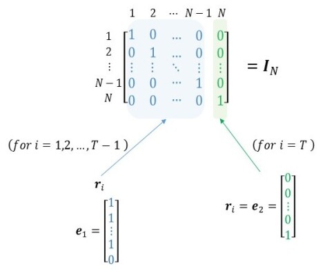
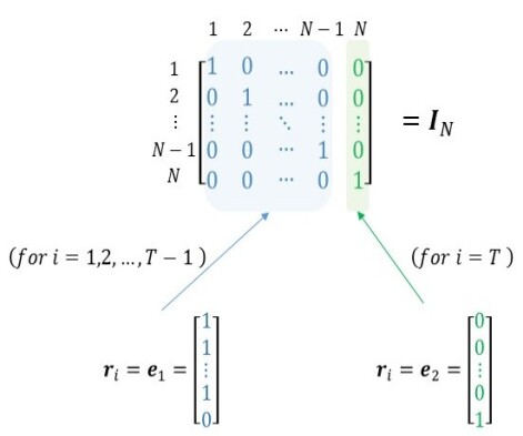
Figure 4: Design of $r_{i}$ and $e_{i}$: (left) for $M_{r}=N$, and (right) for r $M_{r}=N-1$.

Furthermore, for $i=1,...,T-1$ and $i\neq t_{2}$ ($t_{2}$ denoting the time slot that $T_{xA}$ broadcasts to all users in the macrocell), $\mathbf{q}_{i}$ is equal to the submatrix of $\mathbf{I}_{\mathcal{M}_{1}}$ consisting of rows $(M_{r}(i-1)+1,M_{r}i),$ $\mathbf{q}_{T}$ is equal to the submatrix of $\mathbf{I}_{\mathcal{M}}$ consisting of row $\mathcal{M}_{1}$, and $\mathbf{q}_{t_{2}}$ is equal to any one of $\mathbf{q}_{i}$ for $i=1,...,T-1$ and $i\neq t_{2}$. The $t$th component of $\mathbf{\xi}_{i}^{[f_{k}]}$ being 1 means that in the $k$th femtocell, the antennas determined by $\mathbf{r}_{i}$ are in use at time $t$, and the messages determined by $\mathbf{q}_{i}$ are transmitted.

Example 14.

The beamforming matrix for user $f_{1}$, as depicted in Figure 2, is given by:

$$\mathbf{V}_{f_{1}}=\frac{b}{\sqrt{2}}\left(\sum_{i=1}^{3}\mathbf{\mathbf{\xi}}_{i}^{[f_{1}]^{T}}\otimes\mathbf{r}_{i}\mathbf{q}_{i}\right),$$

with

$$\sum_{i=1}^{2}\mathbf{\xi}_{i}^{[f_{1}]}=\mathbf{v}_{1}^{[f_{1}]}=\begin{bmatrix}d&0&d\end{bmatrix},$$

$$\xi_{3}^{[f_{1}]}=\mathbf{v}_{2}^{[f_{1}]}=\begin{bmatrix}0&\sqrt{1-2d^{2}}&0\end{bmatrix}$$

For $i=1,2:$

$$\mathbf{r}_{i}=\mathbf{e}_{1}=\begin{bmatrix}1&0\end{bmatrix}^{T},\;\mathbf{r}_{3}=\mathbf{e}_{2}=\begin{bmatrix}0&1\end{bmatrix}^{T},$$

and $\mathbf{q}_{i}$ the ith unit basis vector where

$$\mathbf{q}_{1}=\mathbf{q}_{2}=\begin{bmatrix}1&0\end{bmatrix},\;\mathbf{q}_{3}=\begin{bmatrix}0&1\end{bmatrix}.$$

v-A Interference Management

In the macrocell projection matrix $\mathbf{P}^{[a_{k}]}$ is given by (40). In each femtocell, in order remove inter-cell interference, the received signal should be projected to a subspace orthogonal to the subspace that inter-cell interference lies in.

Example 15.

For the example model, setting $A=\sqrt{\left(h_{22}^{[f_{1}a_{1}]}\right)^{2}+\left(h_{12}^{[f_{1}a_{1}]}\right)}$ , $B=\sqrt{\left(h_{21}^{[f_{1}a_{1}]}\right)^{2}+\left(h_{11}^{[f_{1}a_{1}]}\right)}$, $\mathbf{P}^{[a_{1}]}$ is given by:

$$\mathbf{P}^{[a_{1}]}={\displaystyle\sum_{s=1}^{2}}\left(\mathbf{w}_{s}^{[a_{k}]}\otimes\left(\mathbf{D}_{s}^{[a_{k}]}\widetilde{\mathbf{h}}^{[f_{k}a_{k}]}\right)\right)$$

where

$$\mathbf{w}_{1}^{[a_{1}]}=\begin{bmatrix}-\sqrt{1-c^{2}}&0&c\end{bmatrix},\;\mathbf{w}_{2}^{[a_{1}]}=\begin{bmatrix}0&1&0\end{bmatrix},$$

$$\mathbf{D}_{1}^{[a_{1}]}=\mathrm{diag}(\begin{bmatrix}0&1\end{bmatrix}^{T}),\;\mathbf{D}_{2}^{[a_{1}]}=\mathrm{diag}(\begin{bmatrix}1&0\end{bmatrix}^{T}),$$ (40)

$$\widetilde{\mathbf{h}}^{[f_{1}a_{1}]}=\begin{bmatrix}\frac{-h_{22}^{[f_{1}a_{1}]}}{A}&\frac{h_{12}^{[f_{1}a_{1}]}}{A}\\ \frac{-h_{21}^{[f_{1}a_{1}]}}{B}&\frac{h_{11}^{[f_{1}a_{1}]}}{B}\end{bmatrix}.$$ (41)

Definition 16.

The rows of the $\mathcal{M}_{1}\times M_{r}T$ projection matrix $\mathbf{P}^{[f_{k}]}$, which is the same for all femtocell users $f_{k}$, form an orthonormal basis of this subspace:

$$\mathbf{P}^{[f_{k}]}=\mathbf{w}\otimes\mathbf{W},$$ (42)

where

1. the $1\times T$ $\mathbf{w}$ is a unit vector orthogonal to $\mathbf{v}^{[a_{i}]}$ for all $i$,

2. and $\mathbf{W}$ is an $\mathcal{M}_{1}\times M_{r}$ all-ones matrix.

Example 17.

For the toy-model, $P^{[f_{1}]}$ is given by:

$$\mathbf{P}^{[f_{1}]}=\mathbf{w}\otimes\mathbf{W}=\left[\frac{1}{\sqrt{1+2c^{2}}}\begin{bmatrix}c&-\sqrt{1-c^{2}}&c&c\end{bmatrix}\otimes\left(\begin{bmatrix}1&1&1\\ 1&1&1\end{bmatrix}^{T}\right)\right],$$

where

$$\mathbf{w}=\frac{1}{\sqrt{1+2c^{2}}}\begin{bmatrix}c&-\sqrt{1-c^{2}}&c&c\end{bmatrix},\;\mathbf{W}=\begin{bmatrix}1&1&1\\ 1&1&1\end{bmatrix}^{T}.$$

Theorem 18.

Multiplying the received signal by projection matrix $\mathbf{P}^{[f_{k}]}$:

$$\mathbf{\widetilde{y}}^{[f_{k}]}=\mathcal{\mathbf{P}}^{[f_{k}]}\mathbf{y}^{[f_{k}]}=\mathcal{\mathbf{\mathcal{H}}}^{[f_{k}]}\mathbf{U}^{[f_{k}]}+\mathbf{\widetilde{Z}}^{[f_{k}]},$$ (43)

where the $\mathcal{M}_{1}\times\mathcal{M}_{1}$ effective channel matrix is given by:

$$\mathcal{\mathbf{\mathcal{H}}}^{[f_{k}]}=\frac{b}{\sqrt{N}}\mathcal{K}^{[f_{k}]}\mathcal{D}^{[f_{k}]},$$ (44)

where

$$\mathcal{K}^{[f_{k}]}=\sqrt{\gamma_{f_{k}}}\mathbf{W}\mathbf{h}^{[f_{k}]},\;\mathcal{D}^{[f_{k}]}={\displaystyle\sum_{i=1}^{T}}\mathbf{w}\xi_{i}^{[f_{k}]^{T}}\mathbf{r}_{i}\mathbf{q}_{i},$$ (45)

and $\mathbf{\widetilde{Z}}^{[f_{k}]}=\mathcal{\mathbf{P}}^{[f_{k}]}\mathbf{Z}^{[f_{k}]}$ remains white noise with the same variance (since $\mathbf{w}$ is a unit vector).

Proof:

We show that $P^{[f_{k}]}$ removes inter-cell interference at the $k$th receiver. Substituting, (18) and (21) in (43), and using $\left(A\otimes B\right)\left(C\otimes D\right)=\left(AC\right)\otimes\left(BD\right)$, the coefficient of $\mathbf{U}^{[a_{i}]}$, for all $i$, becomes:

$$\mathbf{P}^{[f_{k}]}\mathbf{H}^{[Af_{k}]}\mathbf{V}^{[a_{i}]} =\frac{a}{\sqrt{N}}\left(\mathbf{w}\otimes\mathbf{W}\right)\sqrt{\gamma_{a_{1}}}\left(\mathbf{I}_{T}\otimes\mathbf{h}^{[a_{i}]}\right)\left(\mathbf{v}^{[a_{i}]}\otimes\mathbf{I}_{N}\right)$$

$$=\frac{a}{\sqrt{N}}\sqrt{\gamma_{a_{1}}}\left(\mathbf{w}\mathbf{v}^{[a_{i}]}\right)\otimes\left(\mathbf{W}\mathbf{h}^{[a_{i}]}\right),$$ (46)

where by 1) in Definition 16, for all i, $\mathbf{w}\mathbf{v}^{[a_{i}]}=0$, i.e. $\mathbf{w}$ is orthogonal to $\mathbf{v}^{[a_{i}]}$ for all $i$. ∎

v-B Achievable Sum Rate

In the macrocell, the total rate for each user is given by (35). For any channel realization, in the high SNR limit, the rate is maximized for $c=\pm-1/\sqrt{3},$ by maximizing (36).

In each femtocell, since there is no CSIT, the rate for each user, for ONE time slot, is given by:

$$R^{[f_{k}]}=\frac{1}{T}\mathcal{\mathbb{E}}\left[\log\det\left(\mathbf{I}_{\mathcal{M}}+\frac{P_{\mathrm{femtocell}}}{\mathcal{M}\sigma_{n}^{2}}\mathcal{K}^{[f_{k}]}\mathcal{D}^{[f_{k}]}\mathcal{D}^{[f_{k}]^{*}}\mathcal{K}^{[f_{k}]^{*}}\right)\right],$$ (47)

where by taking $\mathrm{det}(\mathcal{D}^{[f_{k}]}\mathcal{D}^{[f_{k}]*})$, the optimal value of $d$ was calculated as $d=\pm 0.5$.

vi Performance Results

Our simulations were based on the example model described and were performed in Matlab. The statistical model chosen was i.i.d. Rayleigh and our input symbols were Quadrature Phase Shift Keying (QPSK) modulated. Maximum-Likelihood (ML) detection was performed in the end of the decoding stage. The total transmit power in the macrocell was considered as $40$W and in the femtocells as $5$W (typical values for transmit power in macrocells for 4G systems), and therefore $a$ and $b$, constants determined by power considerations in (4) and (7) for the hybrid scheme, and (15) and (20) for the Blind IA scheme respectively, are given by $a=\sqrt{40}$ and $b=\sqrt{5}$. Moreover, simulations were performed for $100-500$ frames, with each frame consisting of $6144$ bits.

vi-A Degrees of Freedom

Theorem 19.

For the hybrid scheme, in a heterogeneous network, the total DoF achieved are given by $DoF_{Hybrid}=\frac{KN}{T}(1+L),$ where $K/T$ is the average number of users per group, showing that the less the number of groups is, the more DoF are provided.

Scheme	Macrocell	KL Femtocells	Total Network
Hybrid	$\frac{KN}{T}$	$\frac{KLN}{T}$	$\frac{KN}{T}\left(1+L\right)$
TDMA	$\frac{\left(T-x\right)N}{T}$	$\frac{xKN}{T}$	$\frac{xN\left(K-1\right)+TN}{T}$

Table II: DoF of Hybrid scheme and TDMA.

Theorem 20.

For TDMA, setting $x\in\mathbb{Z}$ and $x<T$, the total DoF achieved are given by $DoF_{TDMA}=\frac{xN\left(K-1\right)+TN}{T}$, where considering a fair time slot allocation to all cells, the DoF will be a function of $x$ which denotes how many time slots will be given to each cell.

Table II presents a comparison between the the hybrid and the TDMA scheme.

Theorem 21.

In a heterogeneous network, as defined in this paper, the hybrid scheme outperforms TDMA in terms of total DoF, as shown in Figure 5 (left). The total DoF gain achieved by the hybrid scheme is given by $DoF_{Hybrid}-DoF_{TDMA}=\frac{N\left(K-1\right)\left(T-x\right)}{T}$.

Proof:

We show that $DoF_{Hybrid}>DoF_{TDMA}$, using $T=L+1$:

$$\frac{KN(1+L)}{T} >\frac{xN\left(K-1\right)+N\left(K-1\right)}{T}$$

$$NT\left(K-1\right) >xN\left(K-1\right)$$

$$T >x,$$ (48)

which is true based on the definition that $x<T$. ∎

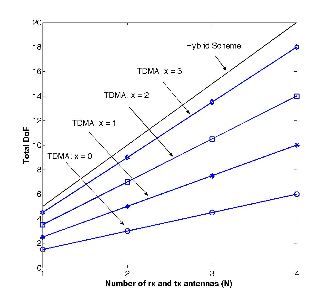
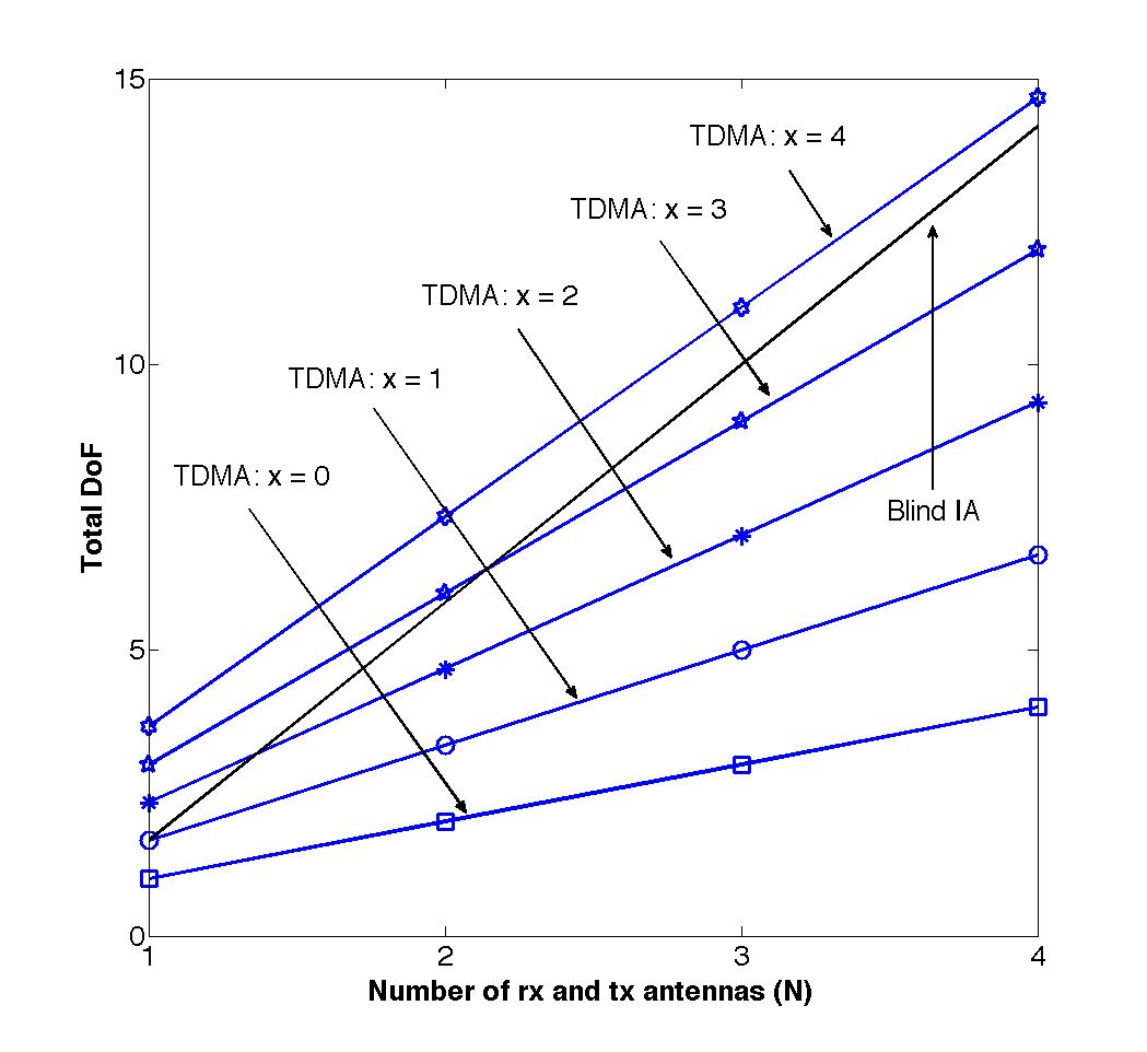
Figure 5: (left) Hybrid Scheme vs. TDMA - Total DoF for $K=5$, $L=3$, $N=\left\{1,2,3,4\right\}$, $x=\left\{0,1,2,3\right\}$ . The hybrid scheme always provides more total DoF. (right) Blind IA vs. TDMA ($L=1$) - Total DoF for $K=5$, $N=M_{r}=\left\{1,2,3,4\right\}$, $x=\left\{0,1,2,3,4\right\}$ . TDMA can outperform Blind IA if more time slots are given to the femtocells.

Theorem 22.

For the Blind IA scheme, in a heterogeneous network, the total DoF achieved are given by $DoF_{Blind\,IA}=K\frac{(N+(K-1)(L-1)(N-L+1)+1)}{T}$, and for the special case $L=1$ where $M_{r}=\left\{N-1,N\right\}$ by $DoF_{Blind\,IA\,L=1}=K\frac{(N+(K-1)(M_{r}-1)+1)}{T}$.

	Scheme	Macrocell	K Femtocells	Total Network
$1<L\leqslant 3$	Blind IA	$\frac{KN}{T}$	$K\frac{((K-1)(L-1)(N-L+1)+1)}{T}$	$K\frac{(N+(K-1)(L-1)(N-L+1)+1)}{T}$
	TDMA $x$ odd	$\frac{\left(T-x\right)N}{T}$	$\frac{\left(\frac{x-1}{2}\right)KNL+K\left(L-1\right)N}{T}$	$\frac{N\left(KL+1\right)+\left(\frac{x-1}{2}\right)KNL-xN}{T}$
	$x$ even		$\frac{\frac{x}{2}KNL}{T}$	$\frac{K\left(N+1\right)+\frac{x}{2}KNL-xN}{T}$
$L=1$	Blind IA	$\frac{KN}{T}$	$K\frac{(K-1)(M_{r}-1)+1}{T}$	$\frac{K(N+(K-1)(M_{r}-1)+1)}{T}$
	TDMA	$\frac{\left(T-x\right)N}{T}$	$\frac{xKM_{r}}{T}$	$\frac{x\left(M_{r}K-N\right)+NT}{T}$

Table III: DoF of Blind IA and TDMA (Scheme B - $L=1$).

Theorem 23.

For TDMA, setting $x\in\mathbb{Z}$ and $x<T$, the total DoF achieved, for $x$ odd and even, are given by $DoF_{TDMA-x\,odd}=\frac{N\left(KL+1\right)+\left(\frac{x-1}{2}\right)KNL-xN}{T}$ and $DoF_{TDMA-x\,even}=\frac{K\left(N+1\right)+\frac{x}{2}KNL-xN}{T}$ respectively, considering a relatively fair time slot allocation to all cells. For the special case $L=1$ where $M_{r}=\left\{N-1,N\right\}$, the DoF are given by $DoF_{TDMA-L=1}=x\left(M_{r}K-N\right)+NT$.

Table III presents a comparison between Blind IA and TDMA.

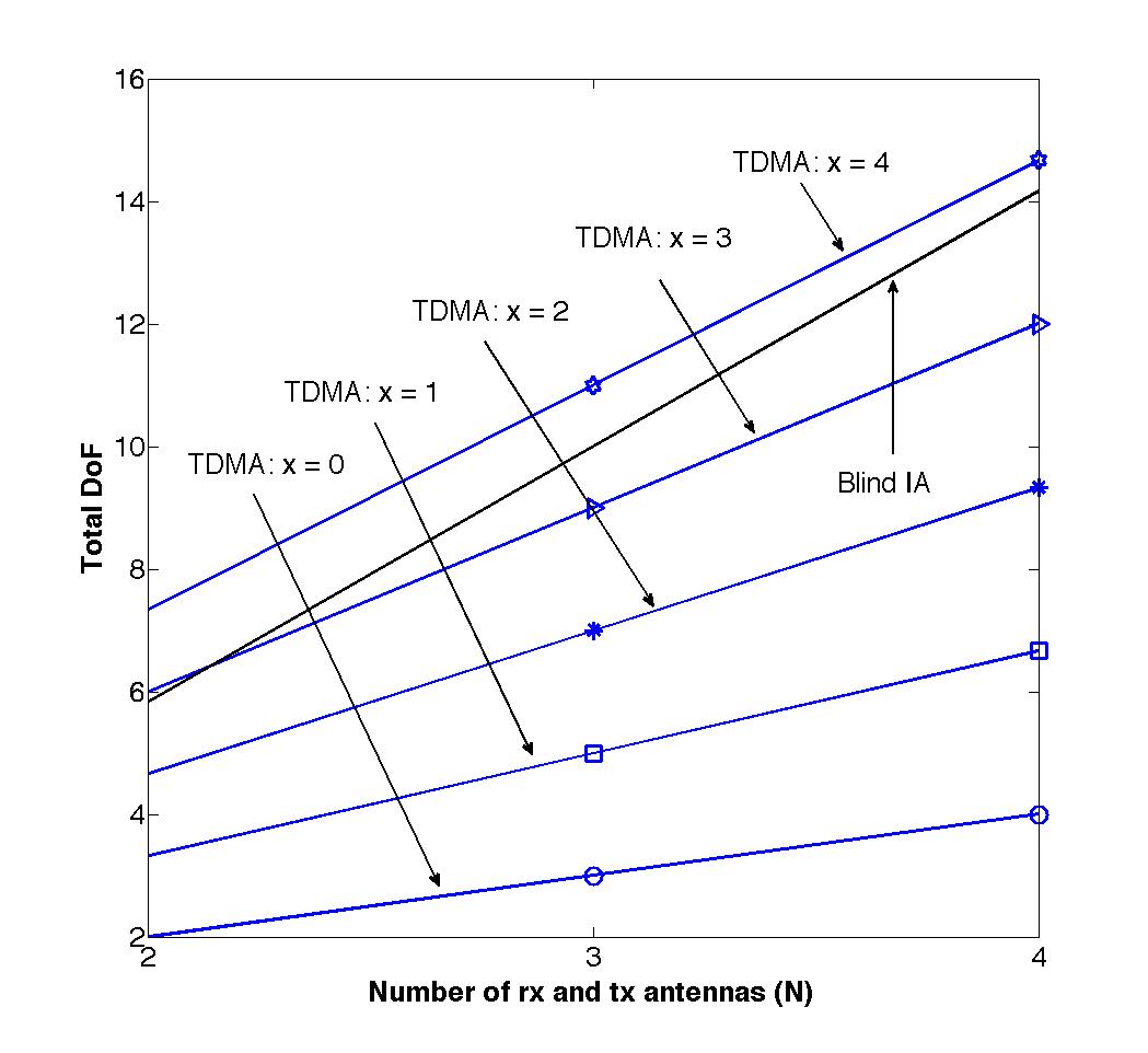
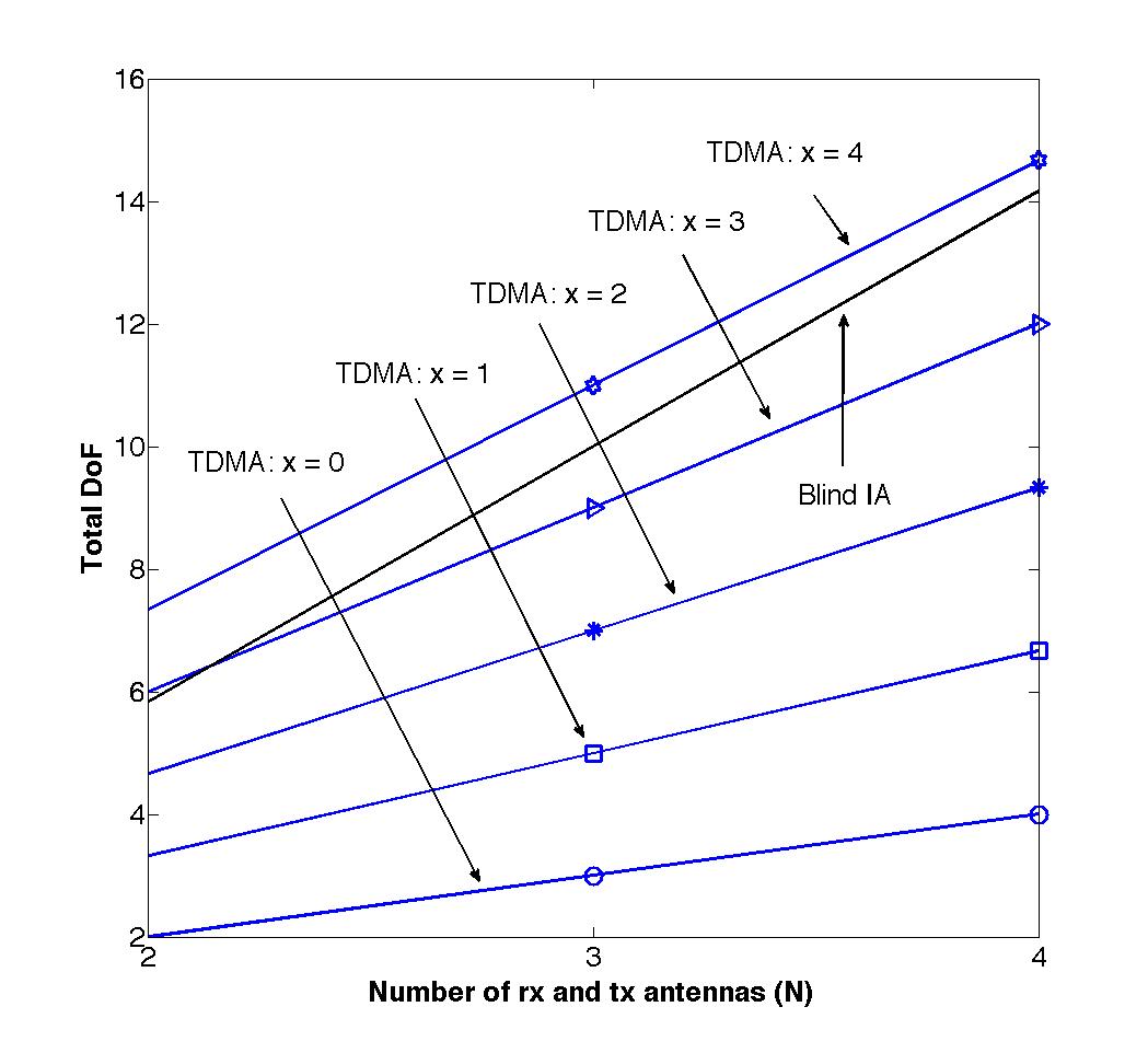
Figure 6: Blind IA vs. TDMA - Total DoF for $K=5$, $L=2$, $N=\left\{2,3,4\right\}$, $x=\left\{0,1,2,3,4\right\}$ for $x$ odd (left) and $x$ even (right). TDMA outperforms Blind IA as more time slots are dedicated to femtocells.

Theorem 24.

For the case that $x$ is odd, the gain of Blind IA to TDMA is given by $DoF_{Blind\,IA}-DoF_{TDMA-x\,odd}=\frac{2K(N+\mathcal{M}_{1}(L-1)+1)-2N(KL+1)-KNL+xN(KL-2)}{2T}$ only when $\frac{2K(N+\mathcal{M}_{1}(L-1)+1)-2N(KL+1)+KNL}{N(KL-2)}>x$. For the case that $x$ is even, the gain of Blind IA is given by $DoF_{Blind\,IA}-DoF_{TDMA-x\,even}=\frac{2K(N+(L-1)\mathcal{M}_{1}+1)-2K(N+1)+xN(KL-2)}{2T}$ only when $\frac{2K(N+\mathcal{M}_{1}(L-1)+1)-2K(N+1)}{N(KL-2)}>x$. For the special case of $L=1$ where $M_{r}=\left\{N-1,N\right\}$, the gain of Blind IA is given by $DoF_{Blind\,IA}-DoF_{TDMA-L=1}=\frac{K(N+(K-1)(M_{r}-1)+1)-NT+x\left(N-M_{r}K\right)}{T}$ only when $\frac{K(N+(K-1)(M_{r}-1)+1)-NT}{M_{r}K-N}>x$.

As shown in Figures 5 (right) and 6, Blind IA outperforms TDMA in the case that we provide more time slots to the macrocell, whereas as the number of time slots dedicated to the femtocells increases, TDMA can achieve more total DoF.

Table IV presents a comparison between the hybrid scheme and the Blind IA. The hybrid scheme outperforms the Blind IA mainly due to the fact that less time slots are required to send the same number of messages. Figure 7 (left) shows that as the number of transmit and receive antennas increases the benefit we get from the hybrid scheme gets smaller, resulting in the Blind IA scheme outperforming the hybrid one for $N>4$. Finally, in Figure 7 (right) it can be seen that as the number of femtocells that interfere with every macrocell user increases, again the benefit we get from the hybrid schemes decreases. However, in general the main advantage of the hybrid scheme is that it overcomes the limitation of the Blind IA scheme that it is valid only for $L\leqslant 3$.

DoF	Total	Example ($L=1$)
Hybrid	$\frac{KN}{T}\left(1+L\right)$	$\mathbf{\frac{8}{2}}$
Blind IA	$K\frac{(N+(K-1)(L-1)(N-L+1)+1)}{T}$	-
Case of $L=1$	$\frac{K(N+(K-1)(M_{r}-1)+1)}{T}$	$\mathbf{\frac{8}{3}}$

Table IV: Comparison of the hybrid scheme and Blind IA Scheme B (Special case: $L=1$). More DoF are provided with the hybrid scheme.

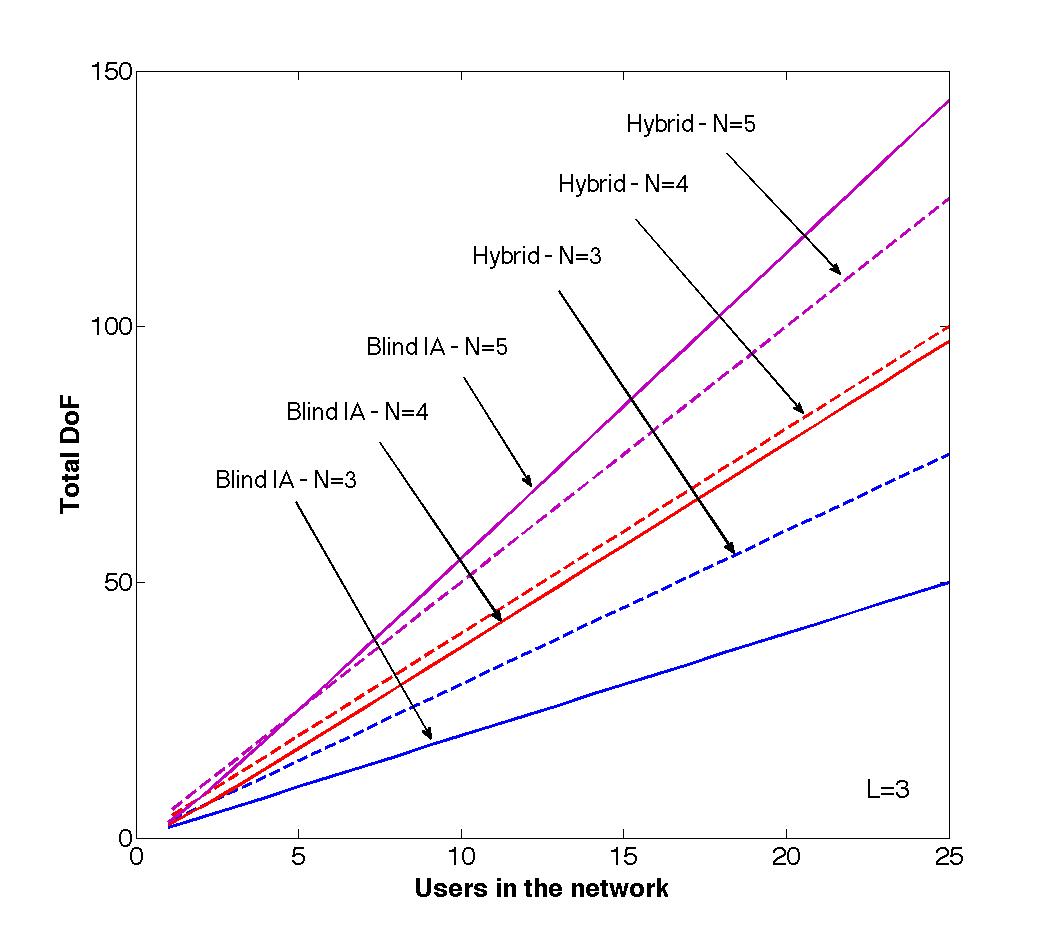
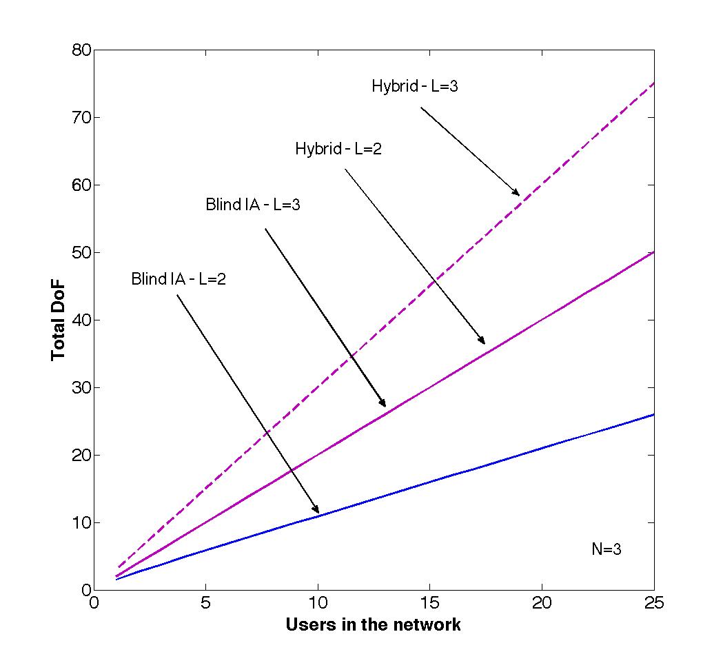
Figure 7: Hybrid Scheme vs. Blind IA - Total DoF for $N=\left\{3,4,5\right\}$, $L=3$ (left) and $L=\left\{2,3\right\}$, $N=3$ (right).

vi-B Bit Error Rate (BER) Performance

First of all, the BER performance of our example model was investigated. In general, since we are considering the distance of every user from the transmitter, users closer to the base station will achieve a better performance than those at the edge of the cell.

Both schemes were first compared to the case where only one user is active in the heterogeneous network (TDMA). Therefore, the BER of every user, both in the macrocell and femtocells, was simulated assuming that only them will receive message over $T=2$ and $T=3$ time slots for the hybrid scheme and Blind IA respectively. Figure 8 (left) depicts the BER for every user separately, for both the hybrid and the TDMA schemes. Note that the BER for users $a_{1}$, $f_{1}$ and $f_{2}$ is 0 for the range of SNR values. Focusing on the total network BER for the hybrid scheme and the average BER for the case of only one user in the network being active, we can observe that both schemes offer similar overall BER performances, with the average TDMA BER slightly outperforming the hybrid scheme for high SNR values. Figure 8 (right) depicts the BER for every user separately, for both the hybrid and the TDMA schemes. Focusing on the total network BER for the hybrid scheme and the average BER for the case of only one user in network being active, we can observe that both schemes offer similar overall BER performances.

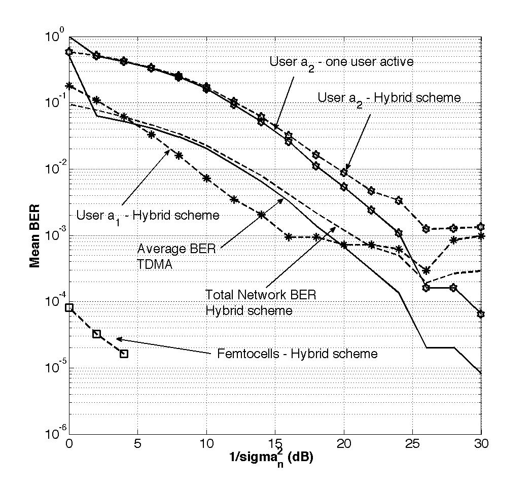
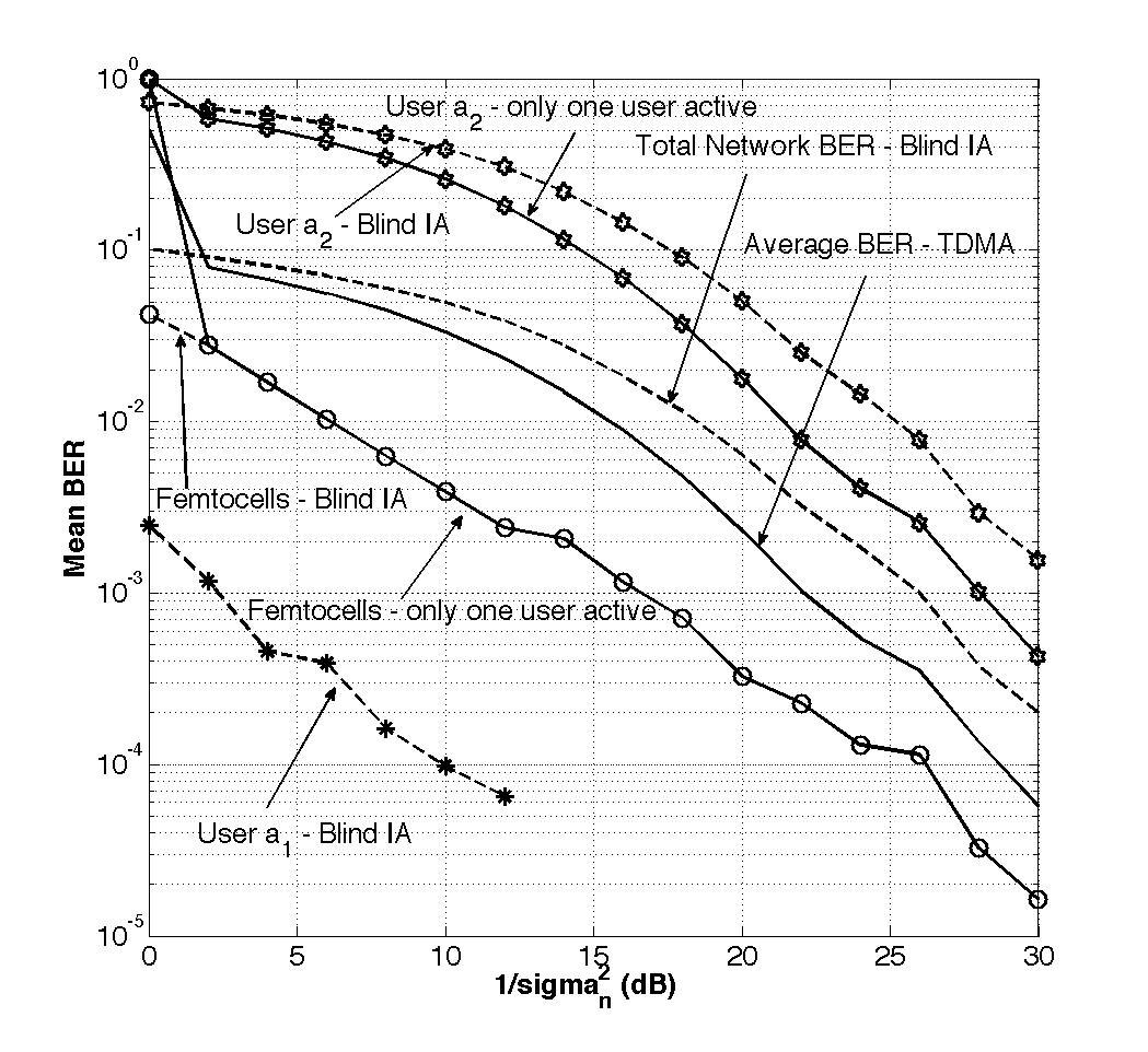
Figure 8: BER Performance: (left) Hybrid vs. TDMA - Total DoF for $K=5$, $L=2$, $N=\left\{2,3,4\right\}$, $x=\left\{0,1,2,3,4\right\}$ for $x$ odd (left) and $x$ even (right) Blind IA vs. TDMA. TDMA outperforms Blind IA as more time slots are dedicated to femtocells

The hybrid scheme was compared to the Blind IA scheme, although a completely fair comparison is not possible, since Blind IA requires $T=3$ time slots and the hybrid scheme $T=2$ time slots (the noise was not the same for the two models), and power allocation is different. However, path loss and channel gains were considered the same. Figure 9 (left) depicts the BER performance of the two schemes, showing that the BER for the macrocell users is better with the scheme of Blind IA, whereas the BER performance in the femtocells, which is 0 for the range of SNR values, is improved with the hybrid scheme. Moreover, in the case of the hybrid scheme, for high SNR values the BER performance of the two users in the macrocell is almost the same, offering fairness and QoS to the edge-cell users. Overall, looking at the total mean BER, the hybrid scheme outperforms Blind IA.

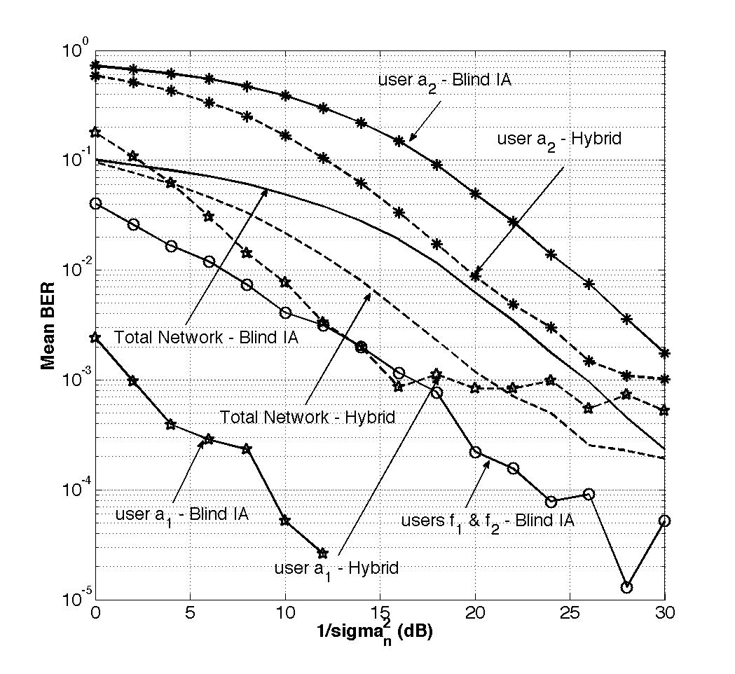
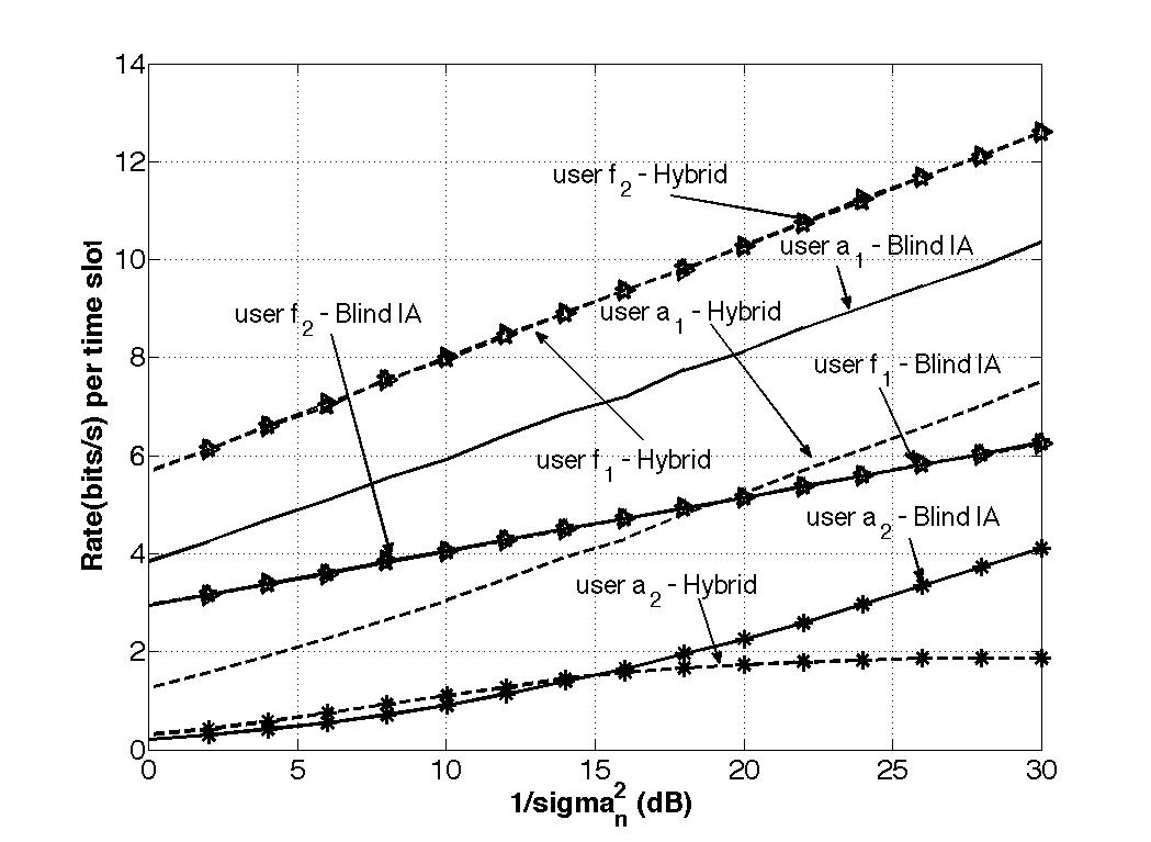
Figure 9: Hybrid Scheme vs. Blind IA - (left) BER Performance, (right) Sum rate Performance. Users in the macrocell can achieve better performance with Blind IA. Users in femtocells achieve better performance with the hybrid scheme

vi-C Rate Performance

The rate of the network will be a function of the user’s distance from the base station and the amount of interference considered as noise (in the case of the hybrid scheme). Again, users closer to the transmitter can achieve higher rates compared to users at the edge of the cell.

Initially both schemes were compared to the case where only one user is active (TDMA) using the following formulas for TDMA:

$$R_{TDMA\,hybrid}^{[a_{k}]}=\frac{1}{T}\mathrm{\mathtt{\mathbb{E}}}\left[\log\det\left(\mathbf{I}_{N}+\frac{P_{\mathrm{macrocell}}}{N\sigma_{n}^{2}}\gamma_{a_{k}}\mathbf{h}_{a_{k}}\mathbf{h}_{a_{k}}^{T}\right)\right].$$ (49)

$$R_{TDMA\,hybrid}^{[f_{kl}]}=\frac{1}{T}\mathcal{\mathbb{E}}\left[\log\det\left(\mathbf{I}_{\mathcal{M}_{1}}+\frac{P_{\mathrm{femtocell}}}{N\sigma_{n}^{2}}\gamma_{f_{kl}}\mathbf{h}_{f_{kl}}\mathbf{h}_{f_{kl}}^{T}\right)\right].$$ (50)

$$R_{TDMA\,BlindIA}^{[a_{k}]}=\frac{1}{T}\mathrm{\mathtt{\mathbb{E}}}\left[\log\det\left(\mathbf{I}_{N}+\frac{P_{\mathrm{macrocell}}}{N^{2}\sigma_{n}^{2}}\mathcal{D}^{[a_{k}]}\mathcal{K}^{[a_{k}]}\mathcal{K}^{[a_{k}]^{*}}\mathcal{D}^{[a_{k}]^{*}}\right)\right].$$ (51)

$$R_{TDMA\,BlindIA}^{[f_{kl}]}=\frac{1}{T}\mathcal{\mathbb{E}}\left[\log\det\left(\mathbf{I}_{\mathcal{M}_{1}}+\frac{P_{\mathrm{femtocell}}}{\mathcal{M}_{1}\sigma_{n}^{2}}\mathcal{K}^{[f_{kl}]}\mathcal{D}^{[f_{kl}]}\mathcal{D}^{[f_{kl}]^{*}}\mathcal{K}^{[f_{kl}]^{*}}\right)\right].$$ (52)

Figure 10 (left) depicts the BER for every user separately, for both the hybrid and the TDMA schemes. Note that the BER for users $a_{1}$, $f_{1}$ and $f_{2}$ is 0 for the range of SNR values. Focusing on the total network BER for the hybrid scheme and the average BER for the case of only one user in the network being active, we can observe that both schemes offer similar overall BER performances, with the average TDMA BER slightly outperforming the hybrid scheme for high SNR values. Figure 10 (right) depicts the BER for every user separately, for both the hybrid and the TDMA schemes. Focusing on the total network BER for the hybrid scheme and the average BER for the case of only one user in network being active, we can observe that both schemes offer similar overall BER performances.

Figure 9 (right) depicts the comparison, in terms of every user’s rate, between Blind IA and the hybrid scheme. The rate of the macrocell users is better in the Blind IA case, however femtocell users in the case of the hybrid scheme achieve higher rates.

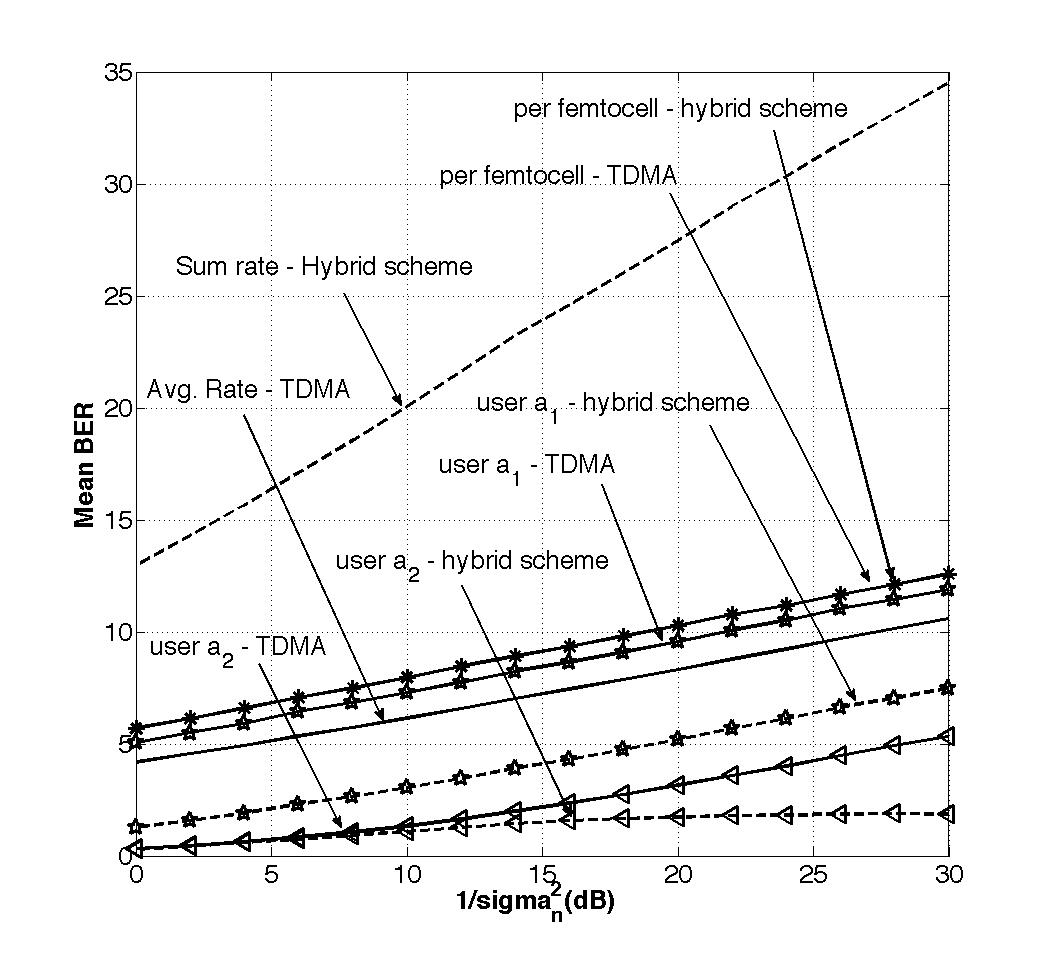
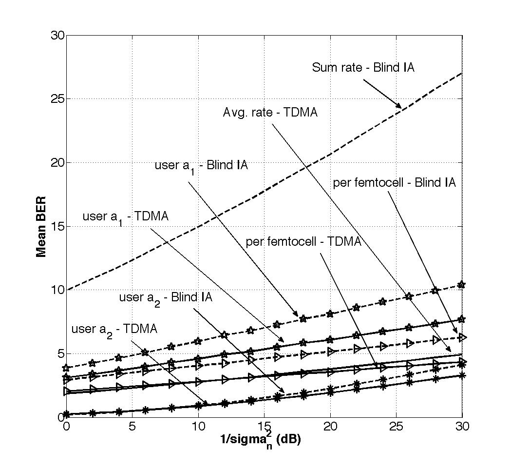
Figure 10: Sum Rate Performance: (left) Hybrid vs. TDMA, (right) Blind IA vs. TDMA. Both schemes achieve higher sum rates than TDMA

vii Summary

Overall, this paper introduces two novel management schemes for a heterogeneous networks with $K$-users in the macrocell, and $KL$ femtocells, with $L$ femtocells interfering with every user in the macrocell. The hybrid scheme provides power allocation fairness and QoS to edge cell users, more DoF, and better performance to the femtocell users, whereas Blind IA achieves considerably higher rates and lower BERs for the users in the macrocell. Most importantly, both schemes can achieve at least double the sum rate of TDMA, with the hybrid scheme always achieving more DoF than TDMA. Due to the low system overhead, high data rates, fair power allocation scheme and the heterogeneous nature of both models, both schemes can be considered as candidates for managing interference in 5G multi-tier communication networks, depending on their requirements and architecture. Future work will focus on wireless energy transfer and physical layer security, two key aspects of future mobile networks, in network architectures that employ the two proposed schemes.

viii Acknowledgements

This work was supported by NEC; the Engineering and Physical Sciences Research Council [EP/I028153/1]; and the University of Bristol.

Appendix

Proof:

(Theorem 9) We show that $P^{[a_{k}]}$ removes intra- and inter- cell interference at the $k$th receiver. Substituting, (1) and (16) in (25), we consider coefficients of $\mathbf{U}^{[a_{i}]}$ and $\mathbf{U}^{[f_{kl}]}$ separately. For $i\neq k$, using $\left(A\otimes B\right)\left(C\otimes D\right)=\left(AC\right)\otimes\left(BD\right)$, for intra-cell interference, coefficient of $\mathbf{U}^{[a_{i}]}$ becomes:

$$\mathbf{P}^{[a_{k}]}\mathbf{H}^{[a_{k}]}\mathbf{V}^{[a_{i}]} =\frac{a}{\sqrt{N}}{\displaystyle\sum_{s=1}^{2}}\left(\mathbf{w}_{s}^{[a_{k}]}\otimes\mathbf{D}_{s}^{[a_{k}]}\mathbf{\widetilde{h}}^{[f_{k}a_{k}]}\right)\sqrt{\gamma_{a_{k}}}(\mathbf{I}_{T}\otimes\mathbf{h}^{[a_{k}]})(\mathbf{v}^{[a_{i}]}\otimes\mathbf{I}_{N})$$

$$=\frac{a}{\sqrt{N}}\sqrt{\gamma_{a_{k}}}{\displaystyle\sum_{s=1}^{2}}\left(\mathbf{w}_{s}^{[a_{k}]}\mathbf{v}^{[a_{i}]}\right)\otimes\left(\mathbf{D}_{s}^{[a_{k}]}\mathbf{\widetilde{h}}^{[f_{k}a_{k}]}\mathbf{h}^{[a_{k}]}\right),$$ (53)

where by 1) in Definition 8, for all s, $\mathbf{w}_{s}^{[a_{k}]}\mathbf{v}^{[a_{i}]}=0$, i.e. $\mathbf{w}_{s}^{[a_{k}]}$ is orthogonal to $\mathbf{v}^{[a_{i}]}$ if $i\neq k$. For $i=k$ the remaining term is (27). For inter-cell interference from Group $G_{1}$, coefficient of $\mathbf{U}^{[f_{kl}]}$:

$$\mathbf{P}^{[a_{k}]}\mathbf{H}^{[f_{kl}a_{k}]}\mathbf{V}^{[f_{kl}]} =\frac{b_{A}}{\sqrt{N}}{\displaystyle\sum_{s=1}^{2}}\left(\mathbf{w}_{s}^{[a_{k}]}\otimes\mathbf{D}_{s}^{[a_{k}]}\mathbf{\widetilde{h}}^{[f_{k}a_{k}]}\right)\sqrt{\gamma_{f_{kl}a_{k}}}\left(\mathbf{I}_{T}\otimes\mathbf{h}^{[f_{kl}a_{k}]}\right)\left(\sum_{i=1}^{T-1}\mathbf{\mathbf{\xi}}_{i}^{[f_{k}]^{T}}\otimes\mathbf{r}\mathbf{q}_{i}^{[f_{kl}]}\right)$$

$$=\frac{b_{A}}{\sqrt{N}}\sqrt{\gamma_{f_{kl}a_{k}}}{\displaystyle\sum_{s=1}^{2}{\displaystyle\sum_{i=1}^{T-1}\mathbf{w}_{s}^{[a_{k}]}}}\mathbf{\xi}_{i}^{[f_{k}]^{T}}\otimes\mathbf{D}_{s}^{[a_{k}]}\mathbf{\widetilde{h}}^{[f_{k}a_{k}]}\mathbf{h}^{[f_{kl}a_{k}]}\mathbf{r}\mathbf{q}_{i}^{[f_{kl}]},$$ (54)

where for $\mathbf{s=1}$: the $(\mathbf{D}_{s}^{[a_{k}]}\mathbf{\widetilde{h}}^{[f_{k}a_{k}]}\mathbf{h}^{[f_{kl}a_{k}]}\mathbf{r})=0$. Premultiplying by $\mathbf{D}_{s}^{[a_{k}]}$ selects a row of $\mathbf{\widetilde{h}}^{[f_{k}a_{k}]}$ and post multiplying by $\mathbf{r}$ selects a column of $\mathbf{\widetilde{h}}^{[f_{k}a_{k}]}$, with the resulting row and column being orthogonal by 4) in Definition 8). For $\mathbf{s=2}$: the $(\mathbf{w}_{s}^{[a_{k}]}\mathbf{\xi}_{i}^{[f_{kl}]^{T}})=0$ by 2) in Definition 8. For inter-cell interference from Group $G_{2}$, coefficient of $\mathbf{U}^{[f_{kl}]}$:

$$\mathbf{P}^{[a_{k}]}\mathbf{H}^{[f_{kl}a_{k}]}\mathbf{V}^{[f_{kl}]} =\frac{b_{B}}{\sqrt{N}}{\displaystyle\sum_{s=1}^{2}}\left(\mathbf{w}_{s}^{[a_{k}]}\otimes\mathbf{D}_{s}^{[a_{k}]}\mathbf{\widetilde{h}}^{[f_{k}a_{k}]}\right)\sqrt{\gamma_{f_{kl}a_{k}}}\left(\mathbf{I}_{T}\otimes\mathbf{h}^{[f_{kl}a_{k}]}\right)\left(\mathbf{v}^{[f_{kl}]T}\otimes\mathbf{e}_{2}\right)$$

$$=\frac{b_{B}}{\sqrt{N}}\sqrt{\gamma_{f_{kl}a_{k}}}{\displaystyle\sum_{s=1}^{2}{\displaystyle\mathbf{w}_{s}^{[a_{k}]}}}\mathbf{v}^{[f_{kl}]T}\otimes\mathbf{D}_{s}^{[a_{k}]}\mathbf{\widetilde{h}}^{[f_{k}a_{k}]}\mathbf{h}^{[f_{kl}a_{k}]}\mathbf{e}_{2},$$ (55)

where for $\mathbf{s=1}$: the $(\mathbf{w}_{s}^{[a_{k}]}\mathbf{v}^{[f_{kl}]T})=0$ by 2) in Definition 8. For $\mathbf{s=2}$: the $(\mathbf{D}_{s}^{[a_{k}]}\mathbf{\widetilde{h}}^{[f_{k}a_{k}]}\mathbf{h}^{[f_{kl}a_{k}]}\mathbf{e}_{2})=0$. Premultiplying by $\mathbf{D}_{s}^{[a_{k}]}$ selects a row of $\mathbf{\widetilde{h}}^{[f_{k}a_{k}]}$ and post multiplying by $\mathbf{e}_{2}$ selects a column of $\mathbf{\widetilde{h}}^{[f_{k}a_{k}]}$, with the resulting row and column being orthogonal by 4) in Definition 8). ∎

Proof:

(Theorem 11) We show that $P^{[f_{kl}]}$ removes inter-cell interference at the $kl$th receiver, so coefficient of $\mathbf{U}^{[a_{i}]}$ for all $i$, becomes:

$$\mathbf{P}^{[f_{kl}]}\mathbf{H}^{[Af_{kl}]}\sum_{i=1}^{K}\mathbf{V}^{[a_{i}]} =\frac{a}{\sqrt{N}}\left(\mathbf{w}\otimes\mathbf{W}^{[f_{kl}]}\right)\sqrt{\gamma_{Af_{kl}}}\left(\mathbf{I}_{T}\otimes\mathbf{h}^{[Af_{kl}]}\right)\left(\sum_{i=1}^{K}\mathbf{v}^{[a_{i}]}\otimes\mathbf{I}_{N}\right)$$

$$=\frac{a}{\sqrt{N}}\sqrt{\gamma_{Af_{kl}}}\sum_{i=1}^{K}\left(\mathbf{w}\mathbf{v}^{[a_{i}]}\otimes\mathbf{W}^{[f_{kl}]}\mathbf{h}^{[Af_{kl}]}\right),$$ (56)

where by 1) in Definition 10, for all i, $\mathbf{w}\mathbf{v}^{[a_{i}]}=0$, i.e. $\mathbf{w}$ is orthogonal to $\mathbf{v}^{[a_{i}]}$ for all $i$. Coefficient of $\mathbf{U}^{[f_{kl}]}$ for $l=2$, becomes:

$$\mathbf{P}^{[f_{kl}]}\mathbf{H}^{[f_{k2}f_{kl}]}\mathbf{V}^{[f_{k2}]} =\frac{b_{B}}{\sqrt{N}}\left(\mathbf{w}\otimes\mathbf{W}^{[f_{kl}]}\right)\sqrt{\gamma_{f_{k2}f_{kl}}}\left(\mathbf{I}_{T}\otimes\mathbf{h}^{[f_{k2}f_{kl}]}\right)\left(\mathbf{v}^{[f_{kl}]^{T}}\otimes\mathbf{e}_{2}\right)$$

$$=\frac{b_{B}}{\sqrt{N}}\sqrt{\gamma_{f_{k2}f_{kl}}}\left(\mathbf{w}\mathbf{v}^{[f_{kl}]^{T}}\otimes\mathbf{W^{[f_{kl}]}}\mathbf{h}^{[f_{k2}f_{kl}]}\mathbf{e}_{2}\right),$$ (57)

where by 2) in Definition 10, $\mathbf{W}^{[f_{kl}]}\mathbf{h}^{[f_{k2}f_{kl}]}\mathbf{e}_{2}=0$. ∎

Proof:

(Theorem 13) We show that $P^{[f_{kl}]}$ removes inter-cell interference at the $kl$th receiver, so coefficient of $\mathbf{U}^{[a_{i}]}$ for all $i$, becomes:

$$\mathbf{P}^{[f_{kl}]}\mathbf{H}^{[Af_{kl}]}\sum_{i=1}^{K}\mathbf{V}^{[a_{i}]} =\frac{a}{\sqrt{N}}\left(\mathbf{w}\otimes\mathbf{W}^{[f_{kl}]}\right)\sqrt{\gamma_{Af_{kl}}}\left(\mathbf{I}_{T}\otimes\mathbf{h}^{[Af_{kl}]}\right)\left(\sum_{i=1}^{K}\mathbf{v}^{[a_{i}]}\otimes\mathbf{I}_{N}\right)$$

$$=\frac{a}{\sqrt{N}}\sqrt{\gamma_{Af_{kl}}}\sum_{i=1}^{K}\left(\mathbf{w}\mathbf{v}^{[a_{i}]}\otimes\mathbf{W}^{[f_{kl}]}\mathbf{h}^{[Af_{kl}]}\right),$$ (58)

where by 1) in Definition 12, for all i, $\mathbf{w}\mathbf{v}^{[a_{i}]}=0$, i.e. $\mathbf{w}$ is orthogonal to $\mathbf{v}^{[a_{i}]}$ for all $i$. Coefficient of $\mathbf{U}^{[f_{kl}]}$ for $l=1,...,L$ and $l\neq 2$, becomes.

$$\mathbf{P}^{[f_{kl}]}\mathbf{H}^{[f_{kl}f_{k2}]}\mathbf{V}^{[f_{kl}]} =\frac{b_{B}}{\sqrt{N}}\left(\mathbf{w}\otimes\mathbf{W}^{[f_{kl}]}\right)\sqrt{\gamma_{f_{kl}f_{k2}}}\left(\mathbf{I}_{T}\otimes\mathbf{h}^{[f_{kl}f_{k2}]}\right)\left(\sum_{i=1}^{T-1}\mathbf{\mathbf{\xi}}_{i}^{[f_{k}]^{T}}\otimes\mathbf{r}\mathbf{q}_{i}^{[f_{kl}]}\right)$$

$$=\frac{b_{B}}{\sqrt{N}}\sqrt{\gamma_{f_{kl}f_{k2}}}\left(\sum_{i=1}^{T-1}\mathbf{w}\mathbf{\xi}^{[f_{kl}]^{T}}\otimes\mathbf{W^{[f_{kl}]}}\mathbf{h}^{[f_{kl}f_{k2}]}\mathbf{r}\mathbf{q}_{i}^{[f_{kl}]}\right),$$ (59)

where by 2) in Definition 12, $\mathbf{W}^{[f_{kl}]}\mathbf{h}^{[f_{kl}f_{k2}]}\mathbf{r}=0$ for $l=1,...,L$ and $l\neq 2$.∎