Initial value problem for the time-dependent linear Schrödinger equation with a point singular potential by the unified transform method

Abstract

We study an initial value problem for the one-dimensional non-stationary linear Schrödinger equation with a point singular potential. In our approach, the problem is considered as a system of coupled initial-boundary value (IBV) problems on two half-lines, to which we apply the unified approach to IBV problems for linear and integrable nonlinear equations, also known as the Fokas unified transform method. Following the ideas of this method, we obtain the integral representation of the solution of the initial value problem.

1 Introduction

The nonlinear Schrödinger (NLS) equation with an external potential $V(x)$ (the so-called Gross-Pitaevskii (GP) equation)

$$iu_{t}+V(x)u+\bigtriangleup u+2\kappa u|u|^{2}=0,\qquad\kappa=\pm 1$$ (1)

is used to describe a lot of phenomena in physics. In particular, it describes the static and dynamical properties of Bose-Einstein condensates, which attracts considerable interest of the researchers after it was experimentally observed in 1995 (see e.g. [19] and the references therein). Also the GP equation is widely used for modelling of superconductors, for describing optical vortices that resemble small twisters in a superfluid, and it appears in the studies of laser beams in Kerr media and focusing nonlinearity [24]. For applications it is desirable to get exact solution of the initial value (IV) problem for equation (1), because it is helpful for describing detailed aspects of a particular physical system, when the approximate methods could be inadequate. But even in one dimension, it is hard to obtain such solutions of the original nonlinear problem.

A reduction of (1) related to short-range interactions consists in replacing $V(x)$ by a point singular potential, which, in the one-dimensional case, is given by $V(x)=q\delta(x)$, $q\in\mathbb{R}$. Assuming that the initial data $u(x,0)=u_{0}(x)$ is an even function, the solution is even for all $t$, and the IV problem

$$\left\{\begin{array}[]{lcl}iu_{t}+u_{xx}+q\delta(x)u+2u|u|^{2}=0,&x>0,\ t>0,\\ u(x,0)=u_{0}(x),&x\geq 0.\\ \end{array}\right.$$ (2)

can be reduced to the initial-boundary value (IBV) problem for the NLS equation without the singular term, with the Robin homogeneous boundary condition, see [10]:

$$\left\{\begin{array}[]{lcl}iu_{t}+u_{xx}+2u|u|^{2}=0,&x>0,\ t>0,\\ u_{x}(0,t)+qu(0,t)=0,&t\geq 0,\\ u(x,0)=u_{0}(x),&x\geq 0.\\ \end{array}\right.$$ (3)

In the latter problem, the boundary conditions are called linearizable, because in this case there exists an adaptation of the Inverse Scattering Transform (IST) method, which turns to be as efficient as the IST method for the initial value problem (on the whole line) (see e.g. [16, 18]). In other words, an initial boundary value problem with linearizable boundary conditions is integrable: the appropriate version of the IST method reduces it to a series of linear problems in a way similar to the problems on the whole line, which in turn allows obtaining detailed information about properties of the solution, e.g., its the long-time behavior.

Particularly, in [10] (see also [17]) the authors have studied in details the long-time behavior of the solution of (3) by applying the nonlinear steepest-descent method for Riemann–Hilbert problems (originally introduced for the whole line problem [9, 11]).

However, if $u_{0}(x)$ is not assumed to be even, (2) does not reduce to (3) and thus the approach of [10] cannot be applied directly.

When analyzing a nonlinear problem, it is natural to solve, first, the associated linearized problem:

$$\left\{\begin{array}[]{lcl}iu_{t}+q\delta(x-a)u+u_{xx}=0,&x\in\mathbb{R},\ t>0,\\ u(x,0)=u_{0}(x),&x\in\mathbb{R}.\\ \end{array}\right.$$ (4)

Problem (4) is the main object of study in the present paper. When trying to reduce (4) to a problem on a half-line, we arrive, instead of (3), at a system of two coupled half-line problems, see (11a) and (11b) below. In other words, we treat the problem (4) as a so-called interface problem, with one interface between two infinite domains. Recall that the interface problems are initial-boundary value problems, for which the boundary conditions depend on the solution of the problems in adjacent domains [8]. These problems have recently attracted considerable attention, see, e.g., [4, 5, 6, 8], where the authors obtained explicit solutions of the original problems by applying the approach known as the Fokas unified transform method (initiated by A.Fokas [12] and successfully developed in the further works, see, e.g., [7, 13, 15]).

The unified transform method is based on the so-called Lax pair representation of an equation in question. Recall that the Lax pair of a given (partial differential) equation is a system of linear ordinary differential equations involving an additional (spectral) parameter, such that the given equation is the compatibly condition of this system. Originally, the Lax pair representation was introduced for certain nonlinear evolution equations, called integrable (see e.g. [1]). This representation plays a key role in solving initial value problems for such equations by the inverse scattering transform (IST) method, where one (spatial) equation from the pair establishes a change of variables, passing from functions of the spatial variable to functions of the spectral parameter, whereas the evolution in time turns out to be, due to the other (temporal) equation from the Lax pair, linear. The Lax pair representation also plays a crucial role in studying initial boundary value problems, where, according to the unified transform method, both equations from the Lax pair are treated in a same manner, as spectral problems.

While only very special (although very important) nonlinear equations have a Lax pair representation (the NLS equation in (3) is one of them), the Lax pair for linear equations with constant coefficients can be constructed algorithmically. Particularly, the Lax pair for the linearized form of the NLS equation, $iu_{t}+u_{xx}=0$, is as follows:

$$\left\{\begin{array}[]{lcl}(\mu e^{-ikx+ik^{2}t})_{x}=ue^{-ikx+ik^{2}t}\\ (\mu e^{-ikx+ik^{2}t})_{t}=(iu_{x}-ku)e^{-ikx+ik^{2}t}\\ \end{array}\right.$$ (5)

Indeed, direct calculations show that the compatibly condition of (5), which is the equality

$$(ue^{-ikx+ik^{2}t})_{t}=((iu_{x}-ku)e^{-ikx+ik^{2}t})_{x}$$

to be satisfied for all $k\in{\mathbb{C}}$, reads $iu_{t}+u_{xx}=0$.

In this paper we obtain an integral representation of the solution of problem (4) using the ideas of the Fokas method (see Theorem 1). Since this method for both linear and integrable nonlinear equations uses the similar ingredients — the Lax pair representation and the analysis of the so-called global relation (see below) — we believe that our results can be useful for studying the initial value problem for the nonlinear Schrödinger equation with a point singular potential.

2 Representation of the solution

In what follows we will consider the initial value problem (4), where $u_{0}(x)$ is a smooth function decaying as $|x|\to\infty$, $a\in\mathbb{R}$ is a parameter, and the solution $u(x,t)$ is assumed to decay to $0$ as $|x|\to\infty$ for all $t>0$ .

First, let us assume that the solution $u(x,t)$ of the problem (4) exists, such that $u(x,t)\in L^{1}({\mathbb{R}})$ and $u_{x}(x,t)\rightarrow 0$ as $|x|\rightarrow\infty$ for all $t$. Our goal is to obtain the (integral) representation for $u(x,t)$ in terms of the given data $u_{0}(x)$.

In order to give exact meaning for (4), we notice that the delta function $2q\delta(x-a)$ is to be understood as introducing the jump condition for the first $x$-derivative:

$$u_{x}(a+0,t)-u_{x}(a-0,t)+2qu(a,t)=0,\qquad t>0$$ (6)

whereas $u(x,t)$ is continuous across $x=a$:

$$u(a+0,t)=u(a-0,t),\qquad t>0.$$ (7)

Thus (4) is to be understood as the following system of equations:

$$\left\{\begin{array}[]{lcl}iu_{t}+u_{xx}=0,&x\in(-\infty,a)\cup(a,\infty),t>0,\\ u(a+0,t)=u(a-0,t),&t>0\\ u_{x}(a+0,t)-u_{x}(a-0,t)+2qu(a,t)=0,&t>0,\\ u(x,0)=u_{0}(x),&x\in(-\infty,\infty)\\ \end{array}\right.$$ (8)

Let’s introduce the notations:

$$\begin{matrix}u^{(1)}(x,t):=\left\{\begin{array}[]{lcl}u(x,t),&x\leq a\\ 0,&x>a\\ \end{array}\right.,&u^{(2)}(x,t):=\left\{\begin{array}[]{lcl}u(x,t),&x\geq a\\ 0,&x<a\\ \end{array}\right.,\end{matrix}$$ (9)

$$\begin{matrix}u^{(1)}_{0}(x):=\left\{\begin{array}[]{lcl}u_{0}(x),&x\leq a\\ 0,&x>a\\ \end{array}\right.,&u^{(2)}_{0}(x):=\left\{\begin{array}[]{lcl}u_{0}(x),&x\geq a\\ 0,&x<a\\ \end{array}\right..\\ \end{matrix}$$ (10)

Then the jump relation can be written as

$$u^{(1)}_{x}(a,t)-qu^{(1)}(a,t)=u^{(2)}_{x}(a,t)+qu^{(2)}(a,t)=:\phi(t),$$

which introduces $\phi(t)$ for $t>0$. On the other hand, the continuity of $u(x,t)$ allows introducing

$$g(t):=u^{(1)}(a,t)=u^{(2)}(a,t).$$

Therefore, the initial value problem (8) can be equivalently written as a pair of coupled initial boundary value problems, with the inhomogeneous boundary conditions:

$$\left\{\begin{array}[]{lcl}iu_{t}^{(1)}+u_{xx}^{(1)}=0,&x<a,\,t>0,\\ u^{(1)}(x,0)=u_{0}^{(1)}(x),&x<a,\\ u_{x}^{(1)}(a,t)-qu^{(1)}(a,t)=\phi(t),&t>0,\\ u^{(1)}(a,t)=g(t),&t>0.\\ \end{array}\right.$$ (11a)

$$\left\{\begin{array}[]{lcl}iu_{t}^{(2)}+u_{xx}^{(2)}=0,&x>a,\,t>0,\\ u^{(2)}(x,0)=u_{0}^{(2)}(x),&x>a,\\ u_{x}^{(2)}(a,t)+qu^{(2)}(a,t)=\phi(t),&t>0,\\ u^{(2)}(a,t)=g(t),&t>0.\\ \end{array}\right.$$ (11b)

We emphasize that neither $\phi(t)$ nor $g(t)$ are given as data for the problems, but (11a) and (11b) are coupled by the condition that these functions are the same for the both problems.

In what follows, we will use the following notations for the direct and inverse Fourier transforms:

$$\mathcal{F}(f)(k)=\hat{f}(k)=\int_{-\infty}^{\infty}e^{-ikx}f(x)\,dx,\,\mathcal{F}^{-1}(\hat{f})(x)=f(x)=\frac{1}{2\pi}\int_{-\infty}^{\infty}e^{ikx}\hat{f}(x)\,dx.$$

With this notations, we define

$$\hat{u}^{(1)}_{0}(k):=\mathcal{F}(u^{(1)}_{0})(x)=\int_{-\infty}^{a}e^{-ikx}u_{0}(x)dx,\qquad\hat{u}^{(2)}_{0}(k):=\mathcal{F}(u^{(2)}_{0})(x)=\int_{a}^{\infty}e^{-ikx}u_{0}(x)dx.$$ (12)

Now, let us assume for a moment that the functions $g(t)$ and $\phi(t)$ are given. Then, using the Lax pair representation separately for the both equations $iu^{(i)}_{t}+u^{(i)}_{xx}=0$, $i=1,2$, we can obtain explicitly the solutions of (11a) and (11b).

Introduce the Fourier-type transforms for the “boundary values” $g(t)$ and $\phi(t)$:

$$\begin{array}[]{lcl}h_{1}(k,t):=\int_{0}^{t}e^{ik^{2}(\tau-t)}g(\tau)\,d\tau,\qquad h_{2}(k,t):=\int_{0}^{t}e^{ik^{2}(\tau-t)}\phi(\tau)\,d\tau.\end{array}$$ (13)

Proposition 1.

The solutions $u^{(j)}(x,t)$, $j=1,2$ of problems (11a) and (11b) can be obtained in terms of $h_{j}(k,t)$ and $\hat{u}^{(j)}_{0}(k)$, $j=1,2$ as follows:

$$u^{(1)}(x,t)=\mathcal{F}^{-1}\left(e^{-ik^{2}t}\hat{u}^{(1)}_{0}(k)+e^{-ika}(iq-k)h_{1}(k,t)+ie^{-ika}h_{2}(k,t)\right),$$ (14)

$$u^{(2)}(x,t)=\mathcal{F}^{-1}\left(e^{-ik^{2}t}\hat{u}^{(2)}_{0}(k)+e^{-ika}(iq+k)h_{1}(k,t)-ie^{-ika}h_{2}(k,t)\right).$$ (15)

Proof.

Consider the Lax pair for equation $iu^{(1)}_{t}+u^{(1)}_{xx}=0$:

$$\left\{\begin{array}[]{lcl}(\mu e^{-ikx+ik^{2}t})_{x}=u^{(1)}e^{-ikx+ik^{2}t}\\ (\mu e^{-ikx+ik^{2}t})_{t}=(iu^{(1)}_{x}-ku^{(1)})e^{-ikx+ik^{2}t}.\\ \end{array}\right.$$ (16)

According to (16), the 1-form

$$W_{1}(x,t,k):=(u^{(1)}e^{-ikx+ik^{2}t})\,dx+((iu_{x}^{(1)}-ku^{(1)})e^{-ikx+ik^{2}t})dt$$

is exact:

$$W_{1}(x,t,k)=d\left[(\mu e^{-ikx+ik^{2}t})\right],\,\,x\leq a,t\geq 0.$$ (17)

It follows that $\oint_{\Gamma}W_{1}(y,\tau,k)=0$, where $\Gamma$ is the rectangle with the vertices $(-X,0)$, $(a,0)$, $(a,t)$, and $(-X,t)$, with any $X>0$, and thus

$$0 = \int_{\Gamma}W_{1}(y,\tau,k)=\oint_{\Gamma}(u^{(1)}e^{-ikx+ik^{2}\tau})\,dx+((iu_{x}^{(1)}-ku^{(1)})e^{-ikx+ik^{2}\tau})\,d\tau$$

$$= \int_{-X}^{a}e^{-ikx}u^{(1)}_{0}(x)\,dx+\int_{0}^{t}e^{-ika+ik^{2}\tau}(iu^{(1)}_{x}(a,\tau)-ku^{(1)}(a,\tau))\,d\tau$$

$$-\int_{-X}^{a}e^{-ikx+ik^{2}t}u^{(1)}(x,t)\,dx-\int_{0}^{t}e^{ikX+ik^{2}\tau}(iu^{(1)}_{x}(-X,\tau)-ku^{(1)}(-X,\tau))\,d\tau.$$

Letting $X\rightarrow+\infty$ in (2) and taking into account the boundary conditions in (11a) and that the last term decays to 0 as $X\rightarrow+\infty$, equation (2) takes the form

$$\hat{u}^{(1)}_{0}(k)+\int_{0}^{t}e^{-ika+ik^{2}\tau}\left[i(\phi(\tau)+qg(\tau))-kg(\tau)\right]\,d\tau-e^{ik^{2}t}\hat{u}^{(1)}(k,t)=0,$$ (19)

which, due to the first term, is valid for all $k$ with $\Im k\geq 0$. Using the notations (13), the last equation can be written as

$$\hat{u}^{(1)}(k,t)=e^{-ik^{2}t}\hat{u}^{(1)}_{0}(k)+e^{-ika}(iq-k)h_{1}(k,t)+ie^{-ika}h_{2}(k,t),\quad\Im k\geq 0,$$ (20)

which implies (14).

The IBV problem for ${u}^{(2)}(x,t)$ can be solved in a similar way, integrating the form $W_{2}$, which is similar to $W_{1}$ with ${u}^{(1)}$ replaced by ${u}^{(2)}$, along the rectangle with the vertices $(X,0)$, $(a,0)$, $(a,t)$, and $(X,t)$ and passing to the limit $X\rightarrow+\infty$. This gives

$$\hat{u}^{(2)}_{0}(k)-e^{ik^{2}t}\hat{u}^{(2)}(k,t)-\int_{0}^{t}e^{-ika+ik^{2}\tau}\left[i(\phi(\tau)-qg(\tau))-kg(\tau)\right]\,d\tau=0,\quad\Im k\leq 0.$$ (21)

Using (13), the last equation can be written as

$$\hat{u}^{(2)}(k,t)=e^{-ik^{2}t}\hat{u}^{(2)}_{0}(k)+e^{-ika}(iq+k)h_{1}(k,t)-ie^{-ika}h_{2}(k,t),\quad\Im k\leq 0,$$ (22)

which implies (15). ∎

Remark 1.

In the framework of the Fokas method, equations (20) and (22) are called the global relations: they relate the “boundary” values of $u(x,\tau)$, taken at $x=a$, $\tau=0$, and $\tau=t$, in the spectral terms, i.e., in the form of the corresponding Fourier-type transforms. The global relations involves given, for a well posed IBV problem, initial/boundary data (in our case, these are the initial data $u_{0}(x)$) as well as unknown boundary values (in our case, these are $g(t)$ and $\phi(t)$). The central importance of the global relations is that they allow to characterize the unknown boundary values in terms of the known (given) ones [2]. While for the IBV problems for nonlinear PDE with non-linearizable boundary conditions, this characterization can be effectively used for studying various aspects of the problem [3, 14, 16] but does not give a “complete” solution to the problem (the expression of the solution in terms of the data for a well-posed problem), in the case of linear PDE this characterization is expected to help solving the IBV completely [13, 15]. Our goal in this paper is actually to demonstrate the latter for problem (8) (or, equivalently, for the coupled problems (11a) and (11b)).

An important feature of the global relations (20) and (22) is the properties of analyticity and decay of their left-hand sides. For linear problems, the analyticity and decay follow directly from their definitions as the Fourier transforms of functions supported on the associated half-lines, which is summarized in the following

Lemma 1.

The functions $h_{i}(k,t)$, $i=1,2$, defined by (13) are analytic in ${\mathbb{C}}$. The function $\hat{u}^{(1)}(k,t)$ is analytic in ${\mathbb{C}}_{+}$ and $\hat{u}^{(2)}(k,t)$ is analytic in ${\mathbb{C}}_{-}$ for all $t\geq 0$, where

$${\mathbb{C}}_{-}:=\{k\in{\mathbb{C}}:\Im k<0\},\qquad{\mathbb{C}}_{+}=\{k\in{\mathbb{C}}:\Im k>0\}.$$ (23)

Moreover, $e^{-ika}\hat{u}^{(1)}(-k,t)$ and $e^{ika}\hat{u}^{(2)}(k,t)$ decay to 0 as $k\to\infty$ in $\bar{\mathbb{C}}_{-}$ (closure of ${\mathbb{C}}_{-}$).

Now observe that, by definition, $h_{i}(k,t)=h_{i}(-k,t)$, $i=1,2$. This observation and Lemma 1 allow rewriting (20) and (22) as a system of equations

$$\left\{\begin{array}[]{lcl}\hat{u}^{(1)}(-k,t)-e^{-ik^{2}t}\hat{u}^{(1)}_{0}(-k)=e^{ika}(iq+k)h_{1}(k,t)+ie^{ika}h_{2}(k,t),\\ \hat{u}^{(2)}(k,t)-e^{-ik^{2}t}\hat{u}^{(2)}_{0}(k)=e^{-ika}(iq+k)h_{1}(k,t)-ie^{-ika}h_{2}(k,t),\end{array}\right.$$ (24)

which holds for all $k\in\bar{\mathbb{C}}_{-}$.

Now suppose for a moment that the functions $\hat{u}^{(i)}(k,t)$, $i=1,2$ are known. Then (24) can be considered as a system of two algebraic equations for two unknown functions $h_{i}(k,t)$. The solution of this system is given for $k\in\bar{\mathbb{C}}_{-}$ by

$$h_{1}(k,t)=\frac{e^{-ika}\left(\hat{u}^{(1)}(-k,t)-e^{-ik^{2}t}\hat{u}_{0}^{(1)}(-k)\right)+e^{ika}\left(\hat{u}^{(2)}(k,t)-e^{-ik^{2}t}\hat{u}_{0}^{(2)}(k)\right)}{2(iq+k)},$$ (25)

$$h_{2}(k,t)=\frac{e^{-ika}\left(\hat{u}^{(1)}(-k,t)-e^{-ik^{2}t}\hat{u}_{0}^{(1)}(-k)\right)-e^{ika}\left(\hat{u}^{(2)}(k,t)-e^{-ik^{2}t}\hat{u}_{0}^{(2)}(k)\right)}{2i}.$$ (26)

Now we are at a position to formulate and prove the main representation result.

Theorem 1.

The solution $u(x,t)$ of problem (8) is given, in terms of the Fourier transforms of the initial data, as follows:

• if $q<0$, then

  $$u(x,t)=\frac{1}{2\pi}\int_{-\infty}^{\infty}e^{ikx-ik^{2}t}\left(\hat{u}_{0}^{(1)}(k)-\frac{iqe^{-2ika}\hat{u}_{0}^{(1)}(-k)-k\hat{u}^{(2)}_{0}(k)}{iq+k}\right)\,dk,$$ (27a)

  for $x<a$, and

  $$u(x,t)=\frac{1}{2\pi}\int_{-\infty}^{\infty}e^{ikx-ik^{2}t}\left(\hat{u}_{0}^{(2)}(k)-\frac{iqe^{-2ika}\hat{u}_{0}^{(2)}(-k)+k\hat{u}_{0}^{(1)}(k)}{iq-k}\right)\,dk,$$ (27b)

  for $x>a$.

• if $q>0$, then

  $$u(x,t)= \frac{1}{2\pi}\int_{-\infty}^{\infty}e^{ikx-ik^{2}t}\left(\hat{u}_{0}^{(1)}(k)-\frac{iqe^{-2ika}\hat{u}_{0}^{(1)}(-k)-k\hat{u}^{(2)}_{0}(k)}{iq+k}\right)\,dk$$

  $$+qe^{q(x-a)+iq^{2}t}\left(\int_{-\infty}^{a}e^{q(y-a)}u_{0}(y)\,dy+\int_{a}^{\infty}e^{-q(y-a)}u_{0}(y)\,dy\right),$$ (27c)

  for $x<a$, and
  

  $$u(x,t)= \frac{1}{2\pi}\int_{-\infty}^{\infty}e^{ikx-ik^{2}t}\left(\hat{u}_{0}^{(2)}(k)-\frac{iqe^{-2ika}\hat{u}_{0}^{(2)}(-k)+k\hat{u}_{0}^{(1)}(k)}{iq-k}\right)\,dk$$

  $$+qe^{-q(x-a)+iq^{2}t}\left(\int_{-\infty}^{a}e^{q(y-a)}u_{0}(y)\,dy+\int_{a}^{\infty}e^{-q(y-a)}u_{0}(y)\,dy\right),$$ (27d)

  for $x>a$.

Remark 2.

The difference in the form of the solution in the cases $q>0$ and $q<0$ is related to the fact that the denominator in (25) has a zero (at $k=-iq$) in the domain ${\mathbb{C}}_{-}$ of validity of (25) in the case $q>0$ only.

Proof.

Since $h_{i}(k,t)=h_{i}(-k,t)$, the first equation in (24) gives the system

$$\left\{\begin{array}[]{lcl}e^{-ika}\left(\hat{u}^{(1)}(-k,t)-e^{-ik^{2}t}\hat{u}^{(1)}_{0}(-k)\right)=(iq+k)h_{1}(k,t)+ih_{2}(k,t),\\ e^{ika}\left(\hat{u}^{(1)}(k,t)-e^{-ik^{2}t}\hat{u}^{(1)}_{0}(k)\right)=(iq-k)h_{1}(k,t)+ih_{2}(k,t),\\ \end{array}\right.$$ (28)

that holds for $k\in\mathbb{R}$, which, getting rid of $h_{2}(k,t)$, leads to the equation

$$e^{-ika}\hat{u}^{(1)}(-k,t)-e^{ika}\hat{u}^{(1)}(k,t)+e^{ika-ik^{2}t}\hat{u}^{(1)}_{0}(k)-e^{-ika-ik^{2}t}\hat{u}^{(1)}_{0}(-k)=2kh_{1}(k,t),\quad k\in\mathbb{R}.$$ (29)

Multiply (29) by $\frac{1}{2\pi}e^{ik(x-a)}$, integrate over $k$ from $-N$ to $N$, and pass to the limit $N\to\infty$. Then for $x<a$, the first terms vanishes due to Lemma 1 and Jordan’s lemma (related to a half-circle in the lower half-plane of $k$) whereas the second term becomes $-u^{(1)}(x,t)$ (as the result of the inverse Fourier transform), and thus the resulting equation is

$$-u^{(1)}(x,t)+\frac{1}{2\pi}\int_{-\infty}^{\infty}e^{ikx-ik^{2}t}\hat{u}^{(1)}_{0}(k)\,dk-\frac{1}{2\pi}\int_{-\infty}^{\infty}e^{ik(x-2a)-ik^{2}t}\hat{u}^{(1)}_{0}(-k)\,dk$$

$$=\frac{1}{2\pi}\int_{-\infty}^{\infty}e^{ik(x-a)}2kh_{1}(k,t)\,dk,\,\,x<a.$$ (30)

Now, in order to obtain $u^{(1)}(x,t)$ in terms of the given (initial) data, we have to express $I_{1}(x,t):=\frac{1}{2\pi}\int_{-\infty}^{\infty}e^{ik(x-a)}2kh_{1}(k,t)\,dk$ for $x<a$ in terms of $u_{0}^{(i)}(x)$. First, we notice that $h_{1}(k,t)$ decays to 0 as $k\to\infty$ in the quadrant $\Re k>0$, $\Im k<0$. Thus, by Jordan’s lemma related to a part of large circle in this quadrant, the integral over the real axis can be deformed to that over the contour $\gamma$, which is shown in Fig. 1:

$$I_{1}(x,t)=\frac{1}{2\pi}\int_{\gamma}e^{ik(x-a)}2kh_{1}(k,t)\,dk,$$ (31)

Substituting (25) into the r.h.s. of (31), we have

$$I_{1}(x,t)=I_{2}(x,t)-I_{3}(x,t),$$

where

$$I_{2}(x,t)=\frac{1}{2\pi}\int_{\gamma}e^{ik(x-a)}k\frac{e^{-ika}\hat{u}^{(1)}(-k,t)+e^{ika}\hat{u}^{(2)}(k,t)}{iq+k}\,dk,$$

and

$$I_{3}(x,t)=\frac{1}{2\pi}\int_{\gamma}e^{ik(x-a)-ik^{2}t}k\frac{e^{-ika}\hat{u}_{0}^{(1)}(-k)+e^{ika}\hat{u}_{0}^{(2)}(k)}{iq+k}\,dk.$$ (32)

Then Lemma 1 and Jordan’s lemma related to a part of big circle in the quadrant $\Re k<0$, $\Im k<0$ implies that $I_{2}(x,t)=0$.

The integral in the r.h.s. of (32) already gives $I_{3}$ (and thus $I_{1}$) in terms of the initial data only. But now we can deform back the integration pass, from $\gamma$ to the real axis, again using Lemma 1 and Jordan’s lemma related to a part of big circle in the quadrant $\Re k>0$, $\Im k<0$, which gives:

• if $q<0$, then

  $$I_{3}(x,t)=\frac{1}{2\pi}\int_{-\infty}^{\infty}e^{ik(x-a)-ik^{2}t}k\frac{e^{-ika}\hat{u}_{0}^{(1)}(-k)+e^{ika}\hat{u}_{0}^{(2)}(k)}{iq+k}\,dk.$$

• if $q>0$, then

  $$I_{3}(x,t)=I_{31}(x,t)+I_{32}(x,t),$$

  where

  $$I_{31}(x,t) =i\underset{k=-iq}{\operatorname{Res}}e^{ik(x-a)-ik^{2}t}k\frac{e^{-ika}\hat{u}_{0}^{(1)}(-k)+e^{ika}\hat{u}_{0}^{(2)}(k)}{iq+k}$$

  $$=qe^{q(x-a)+iq^{2}t}\left(\int_{-\infty}^{a}e^{q(y-a)}u_{0}^{(1)}(y)\,dy+\int_{a}^{\infty}e^{-q(y-a)}u_{0}^{(2)}(y)\,dy\right),$$

  and

  $$I_{32}(x,t)=\frac{1}{2\pi}\int_{-\infty}^{\infty}e^{ik(x-a)-ik^{2}t}k\frac{e^{-ika}\hat{u}_{0}^{(1)}(-k)+e^{ika}\hat{u}_{0}^{(2)}(k)}{iq+k}\,dk.$$

Substituting this into (2) we arrive at the statements of Theorem 1 concerning $u(x,t)$ for $x<a$.

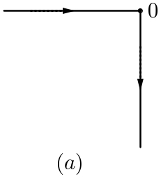
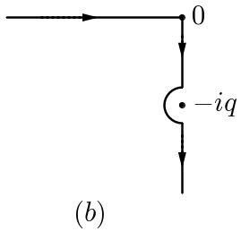
Figure 1: Contour $\gamma$: $(a)$ in the case $q<0$; $(b)$ in the case $q>0$.

To find $u^{(2)}(x,t)$, we proceed in the similar way, with the starting point being the equation (cf. (29)), which follows from the second equation in (24):

$$e^{ika}\hat{u}^{(2)}(k,t)-e^{-ika}\hat{u}^{(2)}(-k,t)+e^{-ika-ik^{2}t}\hat{u}^{(2)}_{0}(-k)-e^{ika-ik^{2}t}\hat{u}^{(2)}_{0}(k)=2kh_{1}(k,t),\quad k\in\mathbb{R}.$$ (33)

Multiply (33) by $\frac{1}{2\pi}e^{ikx}$, integrate over $k$ from $-N$ to $N$, and pass to the limit $N\to\infty$. Then for $x<0$, the first terms vanishes due to Lemma 1 and Jordan’s lemma (related to a half-circle in the lower half-plane of $k$) whereas the second term becomes $-u^{(2)}(a-x,t)$ (again as the result of the inverse Fourier transform):

$$-u^{(2)}(a-x,t)+\frac{1}{2\pi}\int_{-\infty}^{\infty}e^{ik(x-a)-ik^{2}t}\hat{u}^{(2)}_{0}(-k)\,dk-\frac{1}{2\pi}\int_{-\infty}^{\infty}e^{ik(x+a)-ik^{2}t}\hat{u}^{(2)}_{0}(k)\,dk$$

$$=\frac{1}{2\pi}\int_{-\infty}^{\infty}e^{ikx}2kh_{1}(k,t)\,dk,\quad x<0,$$

or

$$-u^{(2)}(x,t)+\frac{1}{2\pi}\int_{-\infty}^{\infty}e^{-ikx-ik^{2}t}\hat{u}^{(2)}_{0}(-k)\,dk-\frac{1}{2\pi}\int_{-\infty}^{\infty}e^{-ik(x-2a)-ik^{2}t}\hat{u}^{(2)}_{0}(k)\,dk$$

$$=\frac{1}{2\pi}\int_{-\infty}^{\infty}e^{-ik(x-a)}2kh_{1}(k,t)\,dk,\quad x>a.$$ (34)

Taking into account that the last term in (2) has already been calculated above, from (2) we obtain

$$u^{(2)}(x,t)=\frac{1}{2\pi}\int_{-\infty}^{\infty}e^{-ikx-ik^{2}t}\hat{u}^{(2)}_{0}(-k)\,dk-\frac{1}{2\pi}\int_{-\infty}^{\infty}e^{-ikx-ik^{2}t}\frac{iqe^{2ika}\hat{u}^{(2)}_{0}(k)-k\hat{u}^{(1)}_{0}(-k)}{iq+k}\,dk,$$ (35)

in the case $q<0$ and

$$u^{(2)}(x,t) = \frac{1}{2\pi}\int_{-\infty}^{\infty}e^{-ikx-ik^{2}t}\hat{u}^{(2)}_{0}(-k)\,dk-\frac{1}{2\pi}\int_{-\infty}^{\infty}e^{-ikx-ik^{2}t}\frac{iqe^{2ika}\hat{u}^{(2)}_{0}(k)-k\hat{u}^{(1)}_{0}(-k)}{iq+k}\,dk$$ (36)

$$+qe^{-q(x-a)+iq^{2}t}\left(\int_{-\infty}^{a}e^{q(y-a)}u_{0}^{(1)}(y)\,dy+\int_{a}^{\infty}e^{-q(y-a)}u_{0}^{(2)}(y)\,dy\right),$$

in the case $q>0$. Substituting $k$ by $-k$ in (35) and (36) we arrive at the statements of the Theorem 1 concerning $u(x,t)$ for $x>a$. ∎

Remark 3.

Setting $x=a$ in (27) gives one part of the “generalized Dirichlet-to-Neumann map”, which has to give unknown boundary values (in the case of problems (11a) and (11b), they are $g(t)$ and $\phi(t)$) in terms of the given data (in our case, they are the initial data $u_{0}(x)$):

$$g(t)=\frac{1}{2\pi}\int_{-\infty}^{\infty}e^{-ik^{2}t}k\frac{e^{-ika}\hat{u}_{0}^{(1)}(-k)+e^{ika}\hat{u}^{(2)}_{0}(k)}{iq+k}\,dk,$$ (37a)

for $$q<0$$, and

$$g(t)= \frac{1}{2\pi}\int_{-\infty}^{\infty}e^{-ik^{2}t}k\frac{e^{-ika}\hat{u}_{0}^{(1)}(-k)+e^{ika}\hat{u}^{(2)}_{0}(k)}{iq+k}\,dk$$

$$+qe^{iq^{2}t}\left(\int_{-\infty}^{a}e^{q(y-a)}u_{0}(y)\,dy+\int_{a}^{\infty}e^{-q(y-a)}u_{0}(y)\,dy\right),$$ (37b)

for $$q>0$$.

In order to obtain the second part of this map, i.e., $\phi(t)$ in terms of $u_{0}(x)$, one can use equation (26) directly following from the global relations. Indeed, multiply (26) by $\frac{k}{\pi}e^{-ik^{2}t^{\prime}}$ with $t^{\prime}<t$, integrate along $\gamma$ and take $t^{\prime}\to t$. Then the l.h.s. gives $\phi(t)$ whereas in the r.h.s, integrating by parts, interchanging the integrals and calculating explicitly the integral $\int_{\gamma}e^{-ikx-ik^{2}t}dk$, one arrives at the representation

$$\phi(t)=\frac{e^{-i\frac{\pi}{4}}}{2\sqrt{\pi t}}\left(\int_{-\infty}^{a}+\int_{a}^{\infty}\right)e^{\frac{i(x-a)^{2}}{4t}}u_{0}^{\prime}(x)\,dx,\quad q\in\mathbb{R}.$$ (38)

for all $q\in\mathbb{R}$.

Remark 4.

Assuming that the initial data $u_{0}(x)$ is a smooth function for $x\in(-\infty,a)\cup(a,\infty)$ decaying fast as $|x|\to\infty$ and matching well the “inner” conditions (6) and (7), i.e.,

$$u_{0}(a-0)=u_{0}(a+0),\quad u^{\prime}_{0}(a+0)-u^{\prime}_{0}(a-0)+2qu_{0}(a)=0,\quad u^{\prime\prime}_{0}(a+0)=u^{\prime\prime}_{0}(a-0)$$ (39)

(the latter condition is suggested by (7) and the equation $iu_{t}+u_{xx}=0$ considered at $x=a\pm 0$) formulas (27) in Theorem 1 give a classical solution to (8).

Indeed, assume that $u_{0}(x)\in C^{4}({\mathbb{R}}\backslash\{a\})\cap C(\mathbb{R})$, $\frac{d^{p}}{dx^{p}}u_{0}(x)\in L^{1}({\mathbb{R}}\setminus\{a\})$ ($p=0,\dots,4$), $x^{j}\frac{d^{4}}{dx^{4}}u_{0}(x)\in L^{1}(\mathbb{R}\setminus\{a\})$ ($j=1,2$), and $u_{0}(x)$ satisfies (39). Then, integrating by parts the definitions (12) of $\hat{u}_{0}^{(j)}(k)$ and taking into account (39), one finds that the integrands in (27) are $O(\frac{1}{k^{4}})$ as $k\to\infty$. It follows that $u(x,t)$ defined by (27) has partial derivatives $u_{t}(x,t)$ and $u_{xx}(x,t)$ in the domains $x<a,t>0$ and $x>a,t>0$ continuous up to the boundaries and satisfying the equation $iu_{t}+u_{xx}=0$. Now, integrating (27) by parts, it follows that $u(x,t)=O\left(\frac{1}{x^{2}}\right)$ and $u_{x}(x,t)=O\left(\frac{1}{x}\right)$ as $|x|\to\infty$. Particularly, $u(x,t)\in L^{1}(\mathbb{R})$ and $u_{x}(x,t)\to 0$ as $|x|\to\infty$.

In order to prove that $u(x,t)$ satisfies the initial condition in (8), we notice that $u(x,0)$ reduces to $\frac{1}{2\pi}\int_{-\infty}^{\infty}e^{ikx}\hat{u}_{0}^{(1)}(k)dk$ for $x<a$ and to $\frac{1}{2\pi}\int_{-\infty}^{\infty}e^{ikx}\hat{u}_{0}^{(2)}(k)dk$ for $x>a$, again applying Lemma 1 and Jordan’s lemma for a circle in ${\mathbb{C}}_{-}$.

Finally, the jump condition in (8) can be proven directly, starting from (27) and using the expressions (37) for $u(a,t)$.

3 The long-time asymptotics

The IST method, particularly, its realization as a Riemann–Hilbert problem method, has proven its high efficiency for studying asymptotic regimes of nonlinear integrable equations, particularly, the long-time behavior of solutions of initial value problems [9, 11] as well as initial boundary value problems (see, e.g., [10]), where the result can be obtained by applying the so-called nonlinear steepest descent method for oscillatory Riemann–Hilbert problems. For linear equations, as far as the solution is given in terms of contour integrals, it is the standard steepest descent method that allows obtaining the asymptotic results. For problem (8), its application leads to the following

Proposition 2.

Let $u_{0}(x)\in L^{1}({\mathbb{R}})$. Then the long-time asymptotics of the solution $u(x,t)$ of problem (8) along any ray $\frac{x}{2t}=\xi$ is as follows:

• if $q<0$, then, as $t\to\infty$,

  $$u(x,t)=\frac{e^{it\xi^{2}-i\frac{\pi}{4}}}{2\sqrt{\pi t}}\left(\hat{u}_{0}^{(1)}(\xi)-\frac{iqe^{-2i\xi a}\hat{u}_{0}^{(1)}(-\xi)-\xi\hat{u}_{0}^{(2)}(\xi)}{iq+\xi}\right)(1+o(1)),$$

  for $x<a$ and

  $$u(x,t)=\frac{e^{it\xi^{2}-i\frac{\pi}{4}}}{2\sqrt{\pi t}}\left(\hat{u}_{0}^{(2)}(\xi)-\frac{iqe^{-2i\xi a}\hat{u}_{0}^{(2)}(-\xi)+\xi\hat{u}_{0}^{(1)}(\xi)}{iq-\xi}\right)(1+o(1)),$$

  for $x>a$.

• if $q>0$, then as $t\to\infty$

  $$u(x,t) =qe^{q(x-a)+iq^{2}t}\left(\int_{-\infty}^{a}e^{q(y-a)}u_{0}(y)\,dy+\int_{a}^{\infty}e^{-q(y-a)}u_{0}(y)\,dy\right)$$

  $$+\frac{e^{it\xi^{2}-i\frac{\pi}{4}}}{2\sqrt{\pi t}}\left(\hat{u}_{0}^{(1)}(\xi)-\frac{iqe^{-2i\xi a}\hat{u}_{0}^{(1)}(-\xi)-\xi\hat{u}_{0}^{(2)}(\xi)}{iq+\xi}\right)(1+o(1)),$$

  for $x<a$ and

  $$u(x,t) =qe^{-q(x-a)+iq^{2}t}\left(\int_{-\infty}^{a}e^{q(y-a)}u_{0}(y)\,dy+\int_{a}^{\infty}e^{-q(y-a)}u_{0}(y)\,dy\right)$$

  $$+\frac{e^{it\xi^{2}-i\frac{\pi}{4}}}{2\sqrt{\pi t}}\left(\hat{u}_{0}^{(2)}(\xi)-\frac{iqe^{-2i\xi a}\hat{u}_{0}^{(2)}(-\xi)+\xi\hat{u}_{0}^{(1)}(\xi)}{iq-\xi}\right)(1+o(1)),$$

  for $x>a$.

4 Concluding remark

In the present paper we have solved the IV problem for the linear Schrödinger equation with a point singular potential by the Fokas unified transform method. Although the initial and initial-boundary value problems for linear equations in $1+1$ dimension could be, in principle, treated by the classical methods (particularly, for the second-order equations), it is important to solve the original problem by the unified transform method, since it is known as providing effective solutions to both linear and nonlinear integrable equations [12, 14, 23]. Therefore, the present paper can be viewed as a step in attacking (particularly, in a perturbative sense [21, 22]) the much more complicated initial value problem for the nonlinear Schrödinger equation with a point singular potential

$$iu_{t}+u_{xx}+q\delta(x)u+2u|u|^{2}=0,$$

in the case of general initial data $u_{0}(x)$ (not assuming it to be an even function). Moreover, the Fokas method is proved to be highly efficient for finding explicit solutions of some interface problems [4, 6, 7, 8]. Therefore, in our paper we have established the applicability of the method for our particular interface problem.

5 Acknowledgments

The author would like to thank D. Shepelsky for many useful conversations and helpful suggestions. The partial support from the Akhiezer Foundation is gratefully acknowledged.

References

[1]
M. J. Ablowitz and H. Segur, Solitons and Inverse Scattering Transform. SIAM Studies
in Applied Mathematics 4. Philadelphia, PA: Society for Industrial and Applied Mathematics
(SIAM), 1981.
[2]
A. Boutet de Monvel, A. S. Fokas, and D.Shepelsky,
Analysis of the global relation for the nonlinear
Schrödinger equation on the half-line,
Lett. Math. Phys. 65, no.3 (2003), 199–212.
[3]
A. Boutet de Monvel, A. S. Fokas, and D.Shepelsky,
Integrable nonlinear evolution equations on a finite interval,
Commun. Math. Phys. 263 (2006), 133–172.
[4]
B. Deconinck and N. Sheils, Interface problems for dispersive equations, Studies in Applied Mathematics, 134(3), (2015), 253-275.
[5]
B. Deconinck and N. Sheils, Initial-to-Interface maps for the heat equation on composite
domains, Studies in Applied Mathematics, 137(1), (2016), 140–154.
[6]
B. Deconinck, N. Sheils, D. Smith, The linear KdV equation with an interface, Communications in Mathematical Physics 347 2 (2016).
[7]
B. Deconinck, T. Trogdon, and V. Vasan, The method of Fokas for solving linear partial
differential equations, SIAM Review , 56(1), (2014), 159–186.
[8]
B. Deconinck, B. Pelloni, and N. Sheils, Non-steady-state heat conduction in composite walls,
Proceedings of the Royal Society A, 470(2165), (2014).
[9]
P. A. Deift, A.R.Its and X. Zhou,
Long-Time asymptotics
for integrable nonlinear wave equations,
in: Important Developments in Soliton Theory, eds. A.S.Fokas and V.E.Zakharov,
Springer, 1993, pp. 181–204.
[10]
P. Deift and J. Park, Long-time asymptotics
for solutions of the NLS equation,
International Mathematics Research Notices (2011), 120 pp.
[11]
P. A. Deift and X. Zhou, A steepest descent method for oscillatory Riemann–Hilbert problems. Asymptotics for the MKdV equation,
Annals of Mathematics 137, no. 2 (1993),
295–368.
[12]
A. S. Fokas, A unified transform method for solving linear and certain
nonlinear PDE’s, Proceedings of the Royal Society A 453 (1997), 1411-1443 .
[13]
A. S. Fokas, A Unified approach to boundary value problems. SIAM, Philadelphia, 2007.
[14]
A. S. Fokas, Integrable nonlinear evolution equations on the half-line,
Communications in Mathematical Physics 230 (2002), 1-39.
[15]
A. Fokas and B. Pelloni. A transform method for linear evolution PDEs on a finite interval.
IMA Journal of Applied Mathematics, 70(4), (2005), 564-587.
[16]
A. S. Fokas, A. R. Its and L. Y. Sung, The nonlinear Schrödinger equation on the half-line.
Nonlinearity 18 (2005), 1771–1822.
[17]
J. Holmer and M. Zvorski, Breathing pattern in nonlinear relaxation, Nonlinearity 22 (2009),
1259–1301.
[18]
A. Its and D. Shepelsky,
Initial boundary value problem for the focusing nonlinear Schrödinger equation with Robin boundary condition: half-line approach,
Proceedings of the Royal Society A 469 (2013), 20120199.
[19]
P. G. Kevrekidis, D. J. Frantzeskakis, R. Carretero-González (eds) Emergent nonlinear phenomena in Bose-Einstein condensates. Atomic, Optical, and Plasma Physics. vol 45. Springer, Berlin, Heidelberg.
[20]
P. D. Lax, Integrals of nonlinear equations of evolution and solitary Waves, Communications on Pure and Applied Mathematics 21 (1968),
467.
[21]
J. Lenells and A. S. Fokas, The unified method: II NLS on the half-line with t-periodic
boundary conditions,
J. Phys. A: Math. Theor. 45 (2012), 195202.
[22]
J. Lenells and A. S. Fokas, The nonlinear Schrödinger equation with t-periodic data: II.
Perturbative results,
Proc. Roy. Soc. A 471 (2015), 20140926.
[23]
B. Pelloni, Advances in the study of boundary value problems for nonlinear integrable PDEs,
Nonlinearity, 28(2) (2015).
[24]
J. Rogel-Salazar, The Gross–Pitaevskii equation and Bose–Einstein condensates, European Journal of Physics 34 (2013).