subref subname = section  thmref thmname = theorem  lemref lemname = lemma 

UWThPh-2015-36

Lukas Schneiderbauer, Harold C. Steinacker

Faculty of Physics, University of Vienna
Boltzmanngasse 5, A-1090 Vienna, Austria

Abstract

We develop a systematic approach to determine and measure numerically the geometry of generic quantum or “fuzzy” geometries realized by a set of finite-dimensional hermitian matrices. The method is designed to recover the semi-classical limit of quantized symplectic spaces embedded in ${\mathds{R}}^{d}$ including the well-known examples of fuzzy spaces, but it applies much more generally. The central tool is provided by quasi-coherent states, which are defined as ground states of Laplace- or Dirac operators corresponding to localized point branes in target space. The displacement energy of these quasi-coherent states is used to extract the local dimension and tangent space of the semi-classical geometry, and provides a measure for the quality and self-consistency of the semi-classical approximation. The method is discussed and tested with various examples, and implemented in an open-source Mathematica package.

1 Introduction

It is generally expected that space-time should have some kind of quantum structure at very short distances. The nature of this quantum structure is not known, and there are many possibilities. One interesting possibility is given by the “matrix” or “quantum” geometry realized by non-trivial solutions of Yang-Mills matrix models, such as the IKKT and BFSS model [1, 2]. These configurations are defined by a set of matrices $X^{a},\ a=1,...,d$, which are interpreted as quantized coordinates in a target space ${\mathds{R}}^{d}$, equipped with the Euclidean metric $\delta_{ab}$ (or $\eta_{ab}$ in the Minkowski case). Prominent examples are the fuzzy sphere $S^{2}_{N}$ [3, 4], fuzzy tori $T^{2}_{N}$, and a wide range of similar spaces which go under the name of “fuzzy spaces”. However this setting is not restricted to group-theoretical spaces, and the general concept is that of quantized symplectic spaces embedded in target space $\mathds{R}^{d}$ [5]. If the underlying manifold is compact, then the $X^{a}$ are realized by finite-dimensional matrices acting on an underlying Hilbert space ${\cal H}\cong{\mathds{C}}^{N}$. These spaces inherit an effective metric structure from their embedding in target space, and they are sufficiently general to realize rather generic 4-dimensional geometries, at least locally.

The main appeal of this matrix model approach is that it provides a natural notion of a “path” integral over the space of geometries, given by the integral over the space of hermitian matrices, with measure defined by the matrix model action. A discussion of some of these aspects can be found in [5].

The aim of the present paper is to use (suitably generalized) coherent states as a tool to understand the quantum geometry defined by such matrix configurations $X^{a},\ a=1,...,d$. We propose a method which allows to distinguish “non-geometric” from “geometric” configurations, and to measure this geometry in some approximate sense. The idea is to look for “optimally localized states” with small dispersion; then the $X^{a}$ can “almost” be simultaneously measured, and their expectation values provide the location of some variety $\mathscr{M}$ embedded in target space $\mathds{R}^{d}$. This allows to assign an approximate notion of geometry even to finite-dimensional matrices, which is meaningful at low energy scales, in a distinctly Wilsonian sense.

Coherent states are well-known for many examples of fuzzy geometries. For quantized coadjoint orbits of compact Lie groups, the basic concept goes back to Perelomov [7], and was reinvented in the specific context of fuzzy spaces [8], cf. [9]. For generic matrix geometries however, the issue of coherent states is less clear. In [10], a concept of coherent states was proposed for geometries realized as a series of matrix algebras, which in the limit recovers the classical space. However, we would like to deal with some fixed, given background geometry, without appealing to some limit. From a physical point of view, this is very natural: the concepts of classical geometry need to emerge only in the low-energy limit, for distances much larger than the scale of noncommutativity (i.e. the Planck scale, presumably). This is all we should expect in physics.

In the present paper, we propose a notion of quasi-coherent states, which is applicable to generic, finite backgrounds. Adapting and generalizing ideas in Berenstein [11] and similar to [10], we define quasi-coherent states as ground states of a matrix Laplacian or a matrix Dirac operator in the presence of a point-like test brane in target space. Their eigenvalues are interpreted as displacement energy $E(\vec{x})$, or as energy of strings stretching between the test brane and the background brane. This string-inspired concept turns out to be very powerful, and independent of more traditional notions in noncommutative geometry such as spectral geometry or differential calculi; it can be seen as a special case of intersecting noncommutative branes [12]. However in contrast to previous work [11, 10], we consider the generic case where this energy is non-vanishing and not constant on the brane. This requires to select a subset of “quasi-minimal” states among all quasi-coherent states, which is achieved by considering the Hessian $H$ of this energy function $E(\vec{x})$. We argue that for matrix backgrounds which define some approximate semi-classical “brane” geometry, the eigenvalues of $H$ must exhibit a clear hierarchy between small eigenvalues $\ll 1$ corresponding to tangential directions, and eigenvalues ${\cal O}(1)$ which correspond to directions transversal to the brane in target space. This hierarchy allows to scan the geometry in a self-consistent way, and to measure the quality of the semi-classical approximation. The resulting quasi-coherent states can then be used to measure the location of the brane in target space, and its geometrical properties similar as in [10, 5].

We discuss two different realizations of this idea, one based on the Laplace operator $\boxempty_{x}$, and one based on a Dirac operator $\not{D}_{x}$. Both arise naturally in the context of Yang-Mills matrix models. The approach based on the Laplace operator is conceptually simpler, but appears less appealing at first because the corresponding ground state energy is strictly positive. Nevertheless, it provides useful information about the local dispersion and geometric uncertainty. The approach using the Dirac operator has the remarkable property that the location of the branes is often recovered from exact zero modes of $\not{D}_{x}$. This property was first pointed out by Berenstein for surfaces in $\mathds{R}^{3}$ [11], but appears to hold much more generally. We discuss this phenomenon in section 7.3, and provide a heuristic argument for the existence of exact zero modes of $\not{D}_{x}$ in a generic setting. On the other hand, this does not provide information about the geometric uncertainty, and we consider both approaches as complementary and equally useful.

The general ideas in this paper are tested and elaborated in detail for the standard examples such as the fuzzy sphere $S^{2}_{N}$, fuzzy torus $T^{2}_{N}$, fuzzy ${\mathds{C}}P^{2}_{N}$, and squashed fuzzy ${\mathds{C}}P^{2}_{N}$. The latter is a very interesting and non-trivial example which arises in ${\cal N}=4$ SYM with a cubic potential [13, 14], and which does not correspond to a Kähler (nor an almost-Kähler) manifold. In particular, we find that the (numerically obtained) quasi-coherent states have smaller dispersion than the Perelomov-type states, and we find strong evidence that the semi-classical geometry is again recovered from exact zero modes of $\not{D}_{x}$. We also find that $\not{D}_{x}$ and $\boxempty_{x}$ lead to slightly different but consistent results for the location of the brane. This can be viewed as a breaking of supersymmetry.

Finally, we provide an implementation of an algorithm in Mathematica, which very nicely reproduces the expected semi-classical geometry of standard examples such as the fuzzy sphere, fuzzy tori, and even degenerate spaces such as squashed fuzzy $\mathds{C}P^{2}$. This algorithm is basically a camera for fuzzy or quantum geometries. It allows to numerically test any given matrix configuration for a possible approximate geometry, to assess the quality of the geometric approximation, and to adjust its “focus” by various parameters. Some pictures taken by this algorithm are reproduced in the paper. We hope that this provides a valuable tool and starting point to explore other unknown quantum geometries, such as those produced by Monte-Carlo simulations of the IIB matrix model [15, 16, 17].

2 Non-commutative (matrix) geometry

Although the methods developed in this paper are more general, we will focus on quantum geometries realized as quantized symplectic manifolds embedded in Euclidean target space. This framework applies to a large class of noncommutative spaces known as fuzzy spaces, which also arise in the matrix-model approach to string theory [1, 2, 18]. Their non-commutative structure can be viewed as quantization of an underlying symplectic manifold, using the same mathematical structures as in quantum mechanics. The metric structure of the geometry is induced by the metric in target space [5].

2.1 Quantization and semi-classical limit

The quantization of a manifold $\mathscr{M}$ with Poisson or symplectic structure amounts to replacing the commutative algebra of functions $\mathscr{C}(\mathscr{M})$ on a manifold with a non-commutative one, and a quantization map $\mathcal{Q}$. For convenience we first recall the concept of a Poisson structure:

Definition 1.

A bilinear map $\{.,.\}:\ \mathscr{C}(\mathscr{M})\times\mathscr{C}(\mathscr{M})\to\mathscr{C}(\mathscr{M})$ which satisfies

• antisymmetry $\{f,g\}=-\{g,f\}$,

• the Leibniz rule $\{f\cdot g,h\}=f\cdot\{g,h\}+\{f,h\}\cdot g$,

• and the Jacobi identity $\{f,\{g,h\}\}+\{g,\{h,f\}\}+\{h,\{f,g\}\}=0$

for all $f,g,h\ \in\mathscr{C}(\mathscr{M})$ is called Poisson structure or Poisson bracket on $\mathscr{M}$. A manifold $\mathscr{M}$ equipped with a Poisson structure is called a Poisson manifold $(\mathscr{M},\{.,.\})$.

For fixed $f\in\mathscr{C}(\mathscr{M})$, the map $\{f,.\}$ is a derivation on $\mathscr{C}(\mathscr{M})$, which defines a (Hamiltonian) vector field on $\mathscr{M}$. We can therefore write the Poisson bracket as bi-vector field in local coordinates,

$$\{f,g\}=\Theta^{\mu\nu}(\partial_{\mu}f)(\partial_{\nu}g),$$ (2.1)

with the usual index conventions. Then $\Theta^{\mu\nu}$ is antisymmetric and obeys the relation

$$\Theta^{\mu\sigma}\partial_{\sigma}\Theta^{\nu\eta}+\Theta^{\nu\sigma}\partial_{\sigma}\Theta^{\eta\mu}+\Theta^{\eta\sigma}\partial_{\sigma}\Theta^{\mu\nu}=0$$ (2.2)

due to the Jacobi identity. If $\Theta^{\mu\nu}$ is non-degenerate, its inverse defines a symplectic structure, i.e. a closed 2-form $\omega\in\Omega^{2}(\mathscr{M})$.

The quantization of such a Poisson or symplectic manifold should be defined in terms of a noncommutative operator algebra $End(\mathscr{H})$ with $\mathscr{H}$ being a Hilbert space, and some way of associating observables to classical function such that the Poisson bracket on $\mathscr{M}$ is recovered as “semi-classical limit” of the commutators in $End(\mathscr{H})$. One way to define a quantization map $\mathcal{Q}$ could be as follows:

Definition 2.

Let $\mathscr{M}$ be a Poisson manifold. A linear map

$$\mathcal{Q}:\mathscr{C}(\mathscr{M})\to End(\mathscr{H})$$ (2.3)

satisfying the axioms

1. $Q(\mathbf{1})=\mathds{1}$,

2. $Q(f)^{\dagger}=Q(f^{*})\quad\forall f\in\mathscr{C}(\mathscr{M})$,

3. correspondence principle:

   $$\lim_{\theta\to\text{0}}\frac{1}{\theta}\big{(}[\mathcal{Q}(f),\mathcal{Q}(g)]-i\mathcal{Q}(\{f,g\}\big{)}=0\quad\forall f,g\in\mathscr{C}(\mathscr{M}),$$ (2.4)

   $$\lim_{\theta\to 0}\big{(}\mathcal{Q}(fg)-\mathcal{Q}(f)\mathcal{Q}(g)\big{)}=0\quad\forall f,g\in\mathscr{C}(\mathscr{M}),$$ (2.5)

4. irreducibility: If $\{f_{i},g\}=0\;\forall i\in I$ implies $g\propto\mathbf{1}$ then $[\mathcal{Q}(f_{i}),A]=0\ \forall i\in I$ implies $A\propto\mathbf{1}$

is called a quantization map. Here $\theta$ is a scale parameter of $\Theta^{\mu\nu}=\theta\bar{\Theta}^{\mu\nu}$.

However, this is somewhat unsatisfactory, since there is in general no unique way to define a quantization map. Moreover, this formulation of the correspondence principle requires a family of quantizations for each $\theta$. In physics, the quantization parameter $\theta$ (or $\hbar$) should be a fixed number, and one is actually faced with the opposite problem of extracting the semi-classical Poisson limit from a given quantum system. If we had a quantization map $\mathcal{Q}$, the semi-classical limit would be obtained by $\mathcal{Q}^{-1}$ in the limit $\theta\to 0$; this will be denoted by the symbol $\sim$. However if $\theta$ is fixed, the answer to this problem can only be approximate, and apply in some scale regime where higher-order contributions of $\hbar$ can be neglected. The required scale in quantum mechanics is set by the Hamiltonian, such as $H=P^{2}+X^{2}$.

Here we want to address the analogous problem: Given some “quantum” or matrix geometry in terms of a set of observables $X^{a}\in End(\mathscr{H})$ (with finite-dimensional $\mathscr{H}$), how can we extract an underlying semi-classical Poisson-manifold? Again the answer can only be approximate, and the extra structure which sets the scale is provided by the metric $\delta_{ab}$ on the target space $\mathds{R}^{d}$. This will allow to extract an effective semi-classical (Riemann-Poisson) geometry from suitable background matrices $X^{a}$.

2.2 Embedded non-commutative (fuzzy) branes

We are interested in the quantum geometry defined in terms of a set of finite-dimensional matrices $X^{a},\ a=1,\ldots,d$. For example, consider a given symplectic manifold embedded in target space,

$$x^{a}:\ \ \mathscr{M}\hookrightarrow\mathds{R}^{d},\qquad a=1,\ldots,d$$ (2.6)

and some quantization $\mathcal{Q}$ thereof along the lines of definition 2. Then define $d$ matrices or operators by

$$X^{a}:=\mathcal{Q}(x^{a})\ \in\ End(\mathscr{H})\ .$$ (2.7)

If $\mathscr{M}$ is compact, these will be finite-dimensional matrices. Our aim is to develop a systematic procedure to reverse this, and to recover approximately the underlying Poisson manifold and its embedding from the $d$ matrices $X^{a}$. Clearly, $\mathcal{Q}$ cannot be injective, but this is physically reasonable and corresponds to an UV-cutoff (as well as an IR cutoff). A formal expansions in $\Theta^{\mu\nu}$ obviously does not make sense, and the algebra $End(\mathscr{H})$ itself contains very little information about the underlying manifold. However, it should still be possible to extract the semi-classical limit in some low-energy regime, corresponding to functions with sufficiently long wave-length. We will see that the Euclidean metric $\delta_{ab}$ on target space $\mathds{R}^{d}$ allows to define a matrix Laplacian and a Dirac operator, which encode the crucial metric information. This will allow to obtain a hierarchy of scales, and to extract the approximate semi-classical geometry in some regime.

Of course, not any set of matrices $\{X^{a}|\,a=1,\ldots,d\}$ will admit such a geometric interpretation, and we should be able to distinguish ”geometric“ configurations from non-geometric ones. We will offer at least a partial answer to this problem, by providing some measures for the quality of a semi-classical approximation.

3 Examples

Let us collect various examples of the above type of embedded quantum geometries, which will serve as testing grounds for our procedure to extract the semi-classical geometry.

3.1 The fuzzy sphere $S^{2}_{N}$

One of the simplest examples is the so called fuzzy sphere [3, 4]. Let us begin with the usual two-sphere

$$\mathscr{M}=S^{2}=\{x\in\mathds{R}^{3}|\sum_{i=1}^{3}x_{i}^{2}=1\}.$$ (3.1)

It has a $SO(3)$ symmetry

$$SO(3)\times S^{2} \to S^{2}$$ (3.2)

$$(g,\vec{x}) \mapsto g\cdot\vec{x},$$

which induces an action on its algebra of functions $\mathscr{C}(S^{2})$

$$SO(3)\times\mathscr{C}(S^{2}) \to \mathscr{C}(S^{2})$$ (3.3)

$$(g,f(\vec{x})) \mapsto (g\triangleright f)(\vec{x}):=f(g^{-1}\cdot\vec{x}).$$

We can then decompose the algebra $\mathscr{C}(S^{2})$ into irreducible representations of $SO(3)$, leading to the well known spherical harmonics $Y_{m}^{l}$

$$\mathscr{C}(S^{2})\doteq\bigoplus_{l=0}^{\infty}\langle\{Y_{m}^{l}|m=-l,\ldots,l\}\rangle.$$ (3.4)

Quantization map.

The quantization is defined such that $\mathcal{Q}:\mathscr{C}(S^{2})\to Mat_{n}(\mathds{C})$ respects this symmetry,

$$\mathcal{Q}(g\triangleright f)=g\triangleright\mathcal{Q}(f)\qquad\forall g\in SO(3),\ f\in\mathscr{C}(S^{2})$$ (3.5)

where $Mat_{n}(\mathds{C})$ is equipped with the $SU(2)$ action

$$SU(2)\times Mat_{n}(\mathds{C}) \to Mat_{n}(\mathds{C})$$ (3.6)

$$(g,M) \mapsto \pi({g})\cdot M\cdot\pi({g})^{-1}.$$

Here $\pi$ denotes the $n$-dimensional irreducible representation (irrep) of $SU(2)$. Then $Mat_{n}(\mathds{C})$ is in general a reducible representation. To decompose it, we recall that $Mat_{n}(\mathds{C})\doteq End(\mathscr{H}_{(n)})\doteq\mathscr{H}_{(n)}\otimes\mathscr{H}_{(n)}^{*}$ as a vector space and also as representation with $\mathscr{H}$ carrying the representation $\pi$. This gives

$$Mat_{n}(\mathds{C})\doteq\mathds{C}^{n}\otimes\mathds{C}^{n*}\doteq(1)\oplus(3)\oplus\ldots\oplus(2n-1)$$ (3.7)

with $(d)$ denoting the $d$-dimensional irrep of $SU(2)$. We define the fuzzy spherical harmonics $\hat{Y}_{m}^{l}$ to be the basis compatible with this decomposition, so that $(2l+1)=\langle\{\hat{Y}_{m}^{l}|m=-l,\ldots,l\}\rangle$. Then we can define a quantization map $\mathcal{Q}$ which preserves the $SO(3)$ symmetry:

$$\mathcal{Q}:\mathscr{C}(S^{2}) \to Mat_{n}(\mathds{C})$$ (3.8)

$$Y_{m}^{l} \mapsto \begin{cases}\hat{Y}_{m}^{l}&l<n-1\\ 0&l\geq n-1\end{cases}$$

It is clear that this map is surjective, and there is a natural built-in momentum cutoff at $l=n-1$.

Embedding functions.

As mentioned before, we are especially interested in the quantized embedding functions $X^{a}\sim x^{a}$. To identify them we note that the embedding functions $x^{i}:\ S^{2}\hookrightarrow\mathds{R}^{3}$ can be identified with the spin 1 spherical harmonics, $Y_{\pm 1}^{1}=x^{1}\pm ix^{2}$ and $Y_{0}^{1}=x^{3}$. Hence their quantization are given by $\hat{Y}_{\pm 1}^{1}=X^{1}\pm iX^{2}$ and $\hat{Y}_{0}^{1}=X^{3}$, or equivalently

$$X^{a}:=\mathcal{Q}(x^{a})=C\,\pi_{(n)}(T^{a})\qquad\in End(\mathscr{H}_{(n)})$$ (3.9)

for some constant $C$, where $T^{a}$ are the generators of $\mathfrak{su}(2)$. It follows that they are the generators of the $n$-dimensional irrep of $SU(2)$, and thus satisfy

$$[X^{a},X^{b}]=i\,C\,\varepsilon_{abc}X^{c}$$ (3.10)

here $\varepsilon_{abc}$ is the Levi-Civita symbol. We fix the radius in the semi-classical limit to be $1$,

$$\sum_{a=1}^{3}(X^{a})^{2}=\mathds{1},$$ (3.11)

which implies $C=2/\sqrt{n^{2}-1}$. Comparing  (LABEL:fuzzysphere_emb) with the correspondence principle in definition 2 one can read off the Poisson structure

$$\{x^{a},x^{b}\}_{S^{2}}=\frac{2}{n}\,\varepsilon_{abc}\,x^{c}$$ (3.12)

which is of order $\theta\sim 1/n$. This corresponds to the unique $SU(2)$-invariant symplectic structure on $S^{2}$ with $\int\omega=2\pi n$.

By considering inductive sequences of fuzzy spheres $(S^{2}_{N})_{N\in{\mathds{N}}}$ with appropriate embeddings, it can be shown that the quantization map axioms defined in (2) are satisfied. However we are interested here in a given, fixed space $S^{2}_{N}$. Then the relation with the classical case is only justified for low angular momenta, consistent with a Wilsonian point of view. One should then only ask for estimates for the deviation from the classical case.

3.2 Fuzzy $\mathds{C}P^{2}_{N}$

The sphere $S^{2}$ can be seen as co-adjoint orbit of the Lie group $SU(2)$. This leads to a large class of generalizations given by quantized coadjoint orbits of semi-simple Lie groups $G$, which can be realized in terms of a matrix algebra $End(\mathscr{H})$ as fuzzy branes embedded in $\mathds{R}^{d}=Lie(G)$. Here we discuss in some detail the complex projective space $\mathds{C}P^{2}$ [20, 21], which is a coadjoint orbit of $SU(3)$; for ${\mathds{C}}P^{n}_{N}$ see e.g. [22].

Co-adjoint orbits.

Let $G$ be a Lie group with Lie algebra $\mathfrak{g}=Lie(G)$. Then $G$ has a natural action on $\mathfrak{g}^{*}$ called the co-adjoint action given by $g\triangleright\mu=\mu(g\cdot.\cdot g^{-1})$ for a $g\in G$ and $\mu\in\mathfrak{g}^{*}$. The co-adjoint orbit $\mathcal{O}_{\mu}^{*}$ of the Lie group $G$ through $\mu\in\mathfrak{g}^{*}$ is then defined as

$$\mathcal{O}_{\mu}^{*}:=\{\mu(g\cdot.\cdot g^{-1})\,|\,g\in G\}.$$ (3.13)

By definition, $\mathcal{O}_{\mu}^{*}$ is invariant under the co-adjoint action. Every orbit of $G$ goes through an element of the dual space of the Cartan algebra $\mathfrak{g}_{0}^{*}$. Co-adjoint orbits carry a natural symplectic form (hence a Poisson structure): The tangent space  $T_{\mu}\mathcal{O}_{\mu}^{*}$ can be identified with $\mathfrak{g}/\mathfrak{K}_{\mu}$ where $\mathfrak{K}_{\mu}$ is the Lie algebra of the stabilizer group $K_{\mu}$ of $\mu$. Then the $G$-invariant symplectic form is

$$\omega_{\mu}(\hat{X},\hat{Y}):=\mu([X,Y])$$ (3.14)

where $\hat{X}$ is the vector field on $\mathfrak{g}^{*}$ generated by the action of $G$. This is an antisymmetric, non-degenerate and closed 2-form on $\mathcal{O}_{\mu}^{*}$.

Let us now consider the case $G=SU(3)$. There are two different types of orbits, depending on the rank of the stabilizer of $\mu$. For the 4-dimensional orbit, we can choose $\mu=t_{8}^{*}$ where

$$t_{8}=\frac{1}{2\sqrt{3}}\begin{pmatrix}1&0&0\\ 0&1&0\\ 0&0&-2\end{pmatrix}.$$

The stabilizer group amounts to $K_{t_{8}^{*}}=SU(2)\times U(1)$, so that the orbit $\mathcal{O}_{t_{8}^{*}}^{*}$ can be characterized as

$$\mathcal{O}_{t_{8}^{*}}^{*}\cong SU(3)/(SU(2)\times U(1)).$$ (3.15)

To see the connection to $\mathds{C}P^{2}$, consider $S^{5}\subset\mathds{C}^{3}$. This carries a natural action of $SU(3)$ by matrix multiplication, which is transitive on $S^{5}$. Then the point $(1,0,0)\in\mathds{C}^{3}$ is stabilized by $SU(2)$, so that

$$S^{5}\cong{SU(3)}/{SU(2)}.$$ (3.16)

On the other hand the complex projective space $\mathds{C}P^{2}$ can be defined as

$$S^{5}/U(1)\cong\mathds{C}P^{2}$$ (3.17)

which is isomorphic to $\mathcal{O}_{t_{8}^{*}}^{*}$ due to (3.15), and points in $\mathcal{O}_{t_{8}^{*}}^{*}$ can be related to the rank one projectors.

Embedding map.

Let $T^{a}$ be an orthonormal basis of $\mathfrak{su}(3)$, which satisfy

$$[T^{a},T^{b}]=ic^{abc}T^{c}$$ (3.18)

where $c^{abc}$ are the structure constants. We can consider them as (Cartesian) coordinate functions on $\mathds{R}^{8}\cong\mathfrak{su}(3)^{*}\ni T=x^{a}t_{a}^{*}$, which describe the embedding

$$x^{a}:\ \mathcal{O}\cong{\mathds{C}}P^{2}\hookrightarrow\mathfrak{su}(3)^{*}\cong\mathds{R}^{8}$$ (3.19)

Since $SU(3)$ is a matrix group, the coadjoint orbit can be characterized through a characteristic equation,

$$T^{*}\in\mathcal{O}_{t_{8}^{*}}^{*}\ \iff\ T\cdot T+\frac{1}{2\sqrt{3}}T-\frac{1}{6}=0$$ (3.20)

which follows easily from the explicit form of $t_{8}^{*}$. Expanding $T=x^{a}t_{a}^{*}$, this gives

$$x^{a}x^{b}d^{abc} = -\frac{1}{\sqrt{3}}x^{c}$$ (3.21)

$$x^{a}x^{b}\delta^{ab} = 1$$

where $d^{abc}$ is the totally symmetric invariant tensor of $\mathfrak{su}(3)$. These equations define the embedding of $\mathds{C}P^{2}$ as $4$-dimensional submanifold in $\mathds{R}^{8}$. One can also characterize the decomposition of the algebra of functions $\mathscr{C}(\mathds{C}P^{2})$ into irreps of $SU(3)$:

$$\mathscr{C}(\mathds{C}P^{2})\doteq\bigoplus_{p=0}^{\infty}\mathscr{H}_{(p,p)}.$$ (3.22)

Here $\mathscr{H}_{(p,p)}$ denotes the irrep of $SU(3)$ with highest weight $(p,p)$.

Quantization map.

As for all coadjoint orbits, the quantized algebra of functions is given by a finite matrix algebra $Mat_{m}(\mathds{C})\cong End(\mathscr{H})$, for an appropriate choice of $\mathscr{H}$. The suitable $\mathscr{H}$ are irreps with highest weight $\Lambda$ proportional to the $\mu$ which determines the coadjoint orbit. In the present case of ${\mathds{C}}P^{2}$, this means that $\mathscr{H}=\mathscr{H}_{(0,n)}$. Then the space of quantized functions

$$End(\mathscr{H}_{(0,n)})\doteq\mathscr{H}_{(0,n)}\otimes\mathscr{H}_{(0,n)}^{*}\doteq\bigoplus_{p=0}^{n}\mathscr{H}_{(p,p)}$$ (3.23)

is isomorphic to (3.22) up to the cutoff $n$. This justifies the above choice of $\mathscr{H}$, and it provides us with a quantization map $\mathcal{Q}$ which is compatible with the $SU(3)$ symmetry,

$$\mathcal{Q}:\ \mathscr{C}(\mathds{C}P^{2}) \to Mat_{m}(\mathds{C})$$ (3.24)

$$Y_{(p,p)}^{\Lambda} \mapsto \begin{cases}\hat{Y}_{(p,p)}^{\Lambda}&p\leq n\\ 0&p>n\ .\end{cases}$$

Here $Y_{(p,p)}^{\Lambda}$ respectively $\hat{Y}_{(p,p)}^{\Lambda}$ is an appropriate basis of the particular $\mathscr{H}_{(p,p)}$, see 3.1b.

(a) $(4,0)$ irrep of $SU(3)$. This triangle form is typical for $(n,0)$ representations. Its size increases with $n$.

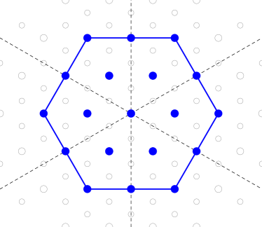
(b) $(2,2)$ irrep of $SU(3)$. All $(n,n)$ representations are of this hexagon form. Its size increases with $n$.

Figure 3.1: Weight space diagrams of $(n,0)$ and $(n,n)$ -type representations of $SU(3)$

Quantized embedding function.

Since the coordinate functions $x^{a}$ transform in the adjoint, the same must hold for the quantized functions $X^{a}$. This means that

$$X^{a}=\mathcal{Q}(x^{a})=C\,\pi_{(0,n)}(T^{a})\qquad\in End(\mathscr{H}_{(0,n)})$$ (3.25)

are nothing but the $\mathfrak{su}(3)$ generators on $\mathscr{H}_{(0,n)}$, which satisfy

$$[X^{a},X^{b}]=i\,C\,c_{abc}X^{c}.$$ (3.26)

Again the constant $C$ will determine the radius of $\mathds{C}P^{2}$ as embedded in ${\mathds{R}}^{8}$. Using the quadratic Casimir operator of $SU(3)$ one sees that setting $C=1/\sqrt{n(1+n/3)}$ yields a $\mathds{C}P^{2}$ with radius $1$ in the semi-classical limit. One can also derive a quantized version of (3.21) [20]. This defines fuzzy $\mathds{C}P_{n}^{2}$ as an embedded fuzzy brane. It is clear that the commutation relations (3.26) should be viewed as quantization of the Poisson bracket $\{x^{a},x^{b}\}=\,C\,c_{abc}x^{c}$ on ${\mathds{C}}P^{2}$, which is precisely the canonical invariant symplectic form discussed above. This concludes for now our brief discussion of fuzzy $\mathds{C}P^{2}$.

The bottom line is that the 8 matrices $X^{a}$ contain enough information to reconstruct the manifold ${\mathds{C}}P^{2}\subset{\mathds{R}}^{8}$ in the semi-classical limit, provided they are interpreted as quantized embedding functions $x^{a}$.

3.3 Squashed $\mathds{C}P^{2}_{N}$

There is a simple modification of $\mathds{C}P_{n}^{2}$, called squashed $\mathds{C}P_{n}^{2}$, which arises as a solution of $\mathcal{N}=4$ supersymmetric Yang-Mills theory with cubic flux term [24]. Recall that fuzzy $\mathds{C}P_{n}^{2}$ is defined by eight matrices $X^{a}=\pi_{(0,n)}(T^{a})$ interpreted as quantized embedding functions $X^{a}\sim x^{a}$, where $T^{a}$ are the generators of $\mathfrak{su}(3)$. Then squashed $\mathds{C}P_{n}^{2}$ is defined by simply dropping two of these matrices corresponding to the Cartan generators, leaving the six matrices $\{X^{a},\,a\in\mathcal{I}=\{1,2,4,5,6,7\}\}$ in the standard Gell-Mann basis. Geometrically, this amounts to a projection in target space

$$\Pi:\ \mathds{R}^{8} \to \mathds{R}^{6}$$ (3.27)

$$(x^{a})_{a=1,\dots,8} \mapsto (x^{a}){}_{a\in\mathcal{I}}$$

resulting in a squashed 4-dimensional variety $\Pi(\mathds{C}P^{2})\hookrightarrow\mathds{R}^{6}$ embedded in $\mathds{R}^{6}$. We will justify below that this interpretation is correct also in the fuzzy case, and we will recover the intricate self-intersecting geometry of squashed $\mathds{C}P^{2}$ in the semiclassical limit both analytically and numerically.

It is worth noting that the Cartan generators $X^{3}$ and $X^{8}$ can be generated by the $X^{a},\,a\in\mathcal{I}$. Therefore the algebra of squashed $\mathds{C}P^{2}_{N}$ is the same matrix algebra as in the non-squashed case.

3.4 Fuzzy torus $T^{2}_{N}$

An example for an embedded brane which does not belong to the class of co-adjoint orbits is the torus $T^{2}=S^{1}\times S^{1}$. It can be embedded in $\mathds{R}^{4}$ via the relations

$$x^{1}+ix^{2}=e^{i\varphi}$$ (3.28)

$$x^{3}+ix^{4}=e^{i\psi}$$

where $\varphi,\psi\in[0,2\pi)$, or more explicitly

$$x:T^{2} \hookrightarrow\mathds{R}^{4}$$ (3.29)

$$(\varphi,\psi) \mapsto\begin{pmatrix}(e^{i\varphi}+e^{-i\varphi})/2\\ -i\,(e^{i\varphi}-e^{-i\varphi})/2\\ (e^{i\psi}+e^{-i\psi})/2\\ -i\,(e^{i\psi}-e^{-i\psi})/2\end{pmatrix}=\begin{pmatrix}\cos(\varphi)\\ \sin(\varphi)\\ \cos(\psi)\\ \sin(\psi)\end{pmatrix}.$$

It is apparent by (LABEL:def_torus) that $T^{2}\subset S^{3}$. Applying a generalized stereographic projection $S^{3}\to\bar{\mathds{R}}^{3}$ (8.15) yields a torus embedded in $\mathds{R}^{3}$ which resembles the usual doughnut form.

It is again useful to identify the symmetry properties of $T^{2}$. The torus carries a $U(1)\times U(1)$ symmetry which acts simply by a multiplication of a phase factor

$$(U(1)\times U(1))\times T^{2} \to T^{2}$$ (3.30)

$$((\Phi,\Psi),(\varphi,\psi)) \mapsto (\varphi+\Phi,\psi+\Psi)$$

which again induces an action on the algebra of functions on the torus $\mathscr{C}(T^{2})$. A basis of $\mathscr{C}(T^{2})$ which respects the symmetry is given by the functions $\phi_{l,k}$:

$$\phi_{l,k}(\varphi,\psi):=e^{il\varphi}e^{ik\psi}.$$ (3.31)

A function $f\in\mathscr{C}(T^{2})$ expanded in this basis, i.e. $f(\varphi,\psi)=\sum_{l,k=-\infty}^{\infty}f_{l,k}\,\phi_{l,k}(\varphi,\psi)$, is nothing but the Fourier series of $f$.

Construction of matrix algebra.

To construct the appropriate quantization in terms of a matrix algebra $Mat_{n}(\mathds{C})$, we introduce the shift matrix $U$ and the clock matrix $V$

$$U=\begin{pmatrix}0&1\\ &0&1\\ &&\ddots&\ddots\\ &&&0&1\\ 1&&&&0\end{pmatrix},\qquad V=\begin{pmatrix}1\\ &q\\ &&q^{2}\\ &&&\ddots\\ &&&&q^{n-1}\end{pmatrix}$$ (3.32)

with $q:=e^{2\pi i/n}$. These are unitary matrices with the property $U^{n}=V^{n}=\mathds{1}$ obeying the commutation relations

$$[U,V]=(q-1)\,VU.$$ (3.33)

It is clear that the set of matrices $\{\mathds{1},U,U^{2},\dots,U^{n}\}$ respectively $\{\mathds{1},V,V^{2},\dots,V^{n}\}$ form a representation of the cyclic group $\mathds{Z}_{n}$. Now define matrices $\Phi_{l,k}$ as

$$\Phi_{l,k}:=U^{l}V^{k}$$ (3.34)

for $l,k\in\{-\frac{n-1}{2},\dots 0,\dots,\frac{n-1}{2}\}$. These are $n^{2}$ linear independent matrices which form a basis of $Mat_{n}(\mathds{C})$. Let us consider now the adjoint action of $\mathds{Z}_{n}\times\mathds{Z}_{n}\subset U(1)\times U(1)$ on $Mat_{n}(\mathds{C})$ given by

$$(\mathds{Z}_{n}\times\mathds{Z}_{n})\times Mat_{n}(\mathds{C}) \to Mat_{n}(\mathds{C})$$ (3.35)

$$((w^{r},w^{s}),M) \mapsto V^{s}\cdot(U^{r}\cdot M\cdot U^{-r})\cdot V^{-s}.$$

We can calculate the action on the basis $\Phi_{l,k}$ using (LABEL:torus_com) and get

$$(w^{r},w^{s})\triangleright\Phi_{l,k}=q^{sl+kr}\,\Phi_{l,k}.$$ (3.36)

Therefore the one-dimensional subspaces spanned by the basis vectors are invariant under the $\mathds{Z}_{n}\times\mathds{Z}_{n}$ action.

Quantization map.

Now it is easy to construct a quantization map $\mathcal{Q}$ which respects the $\mathds{Z}_{n}\times\mathds{Z}_{n}\subset U(1)\times U(1)$ symmetry on our algebras.

$$\mathcal{Q}:\ \mathscr{C}(T^{2}) \to Mat_{n}(\mathds{C})$$ (3.37)

$$\phi_{l,k} \mapsto\begin{cases}q^{-lk/2}\,\Phi_{l,k}&|l|,|k|\leq(n-1)/2\\ 0&\mathrm{otherwise}\end{cases}.$$

The factor $q^{-lk/2}$ is chosen such that $\mathcal{Q}(f^{*})=\mathcal{Q}(f)^{\dagger}$ holds. The appropriate Poisson structure on $\mathscr{C}(T^{2})$ can be guessed from (LABEL:torus_com): Since $[\mathcal{Q}(e^{i\varphi}),\mathcal{Q}(e^{i\psi})]=[U,V]=(q-1)\,UV=(q-1)\,\mathcal{Q}(e^{i\psi})\mathcal{Q}(e^{i\varphi})$ and $q=e^{2\pi i/n}=1+\frac{2\pi i}{n}+\mathcal{O}((\frac{1}{n})^{2})$, the correspondence principle requires that

$$2\pi i\,\mathcal{Q}(e^{i\psi})\mathcal{Q}(e^{i\varphi})=i\lim_{n\to\infty}n\,\mathcal{Q}(\{e^{i\varphi},e^{i\psi}\}),$$ (3.38)

hence $\{e^{i\varphi},e^{i\psi}\}=\frac{2\pi}{n}e^{i\varphi}e^{i\psi}$, and $\mathcal{Q}(fg)\to\mathcal{Q}(f)\mathcal{Q}(g)$ holds as $n\to\infty$. This allows us to conclude

$$\{\varphi,\psi\}_{T^{2}}=-\frac{2\pi}{n}$$ (3.39)

which is obviously $U(1)\times U(1)$ invariant. It is then easy to see that the correspondence principle holds for all quantized functions in the limit $n\to\infty$.

Quantized embedding functions.

We can directly read off the quantized embedding functions $X^{a}=\mathcal{Q}(x^{a})$ from (LABEL:torus_embedding):

$$X^{1} =(U+U^{\dagger})/2$$ (3.40)

$$X^{2} =-i\,(U-U^{\dagger})/2$$

$$X^{3} =(V+V^{\dagger})/2$$

$$X^{4} =-i\,(V-V^{\dagger})/2.$$

3.5 Other types of matrix geometries

The above examples are quantized symplectic spaces with a more-or-less regular immersion in target space. However, there are many interesting examples with degenerate embedding. For example, it turns out that squashed ${\mathds{C}}P^{2}$ has a triple self-intersection at the origin in target space, which leads to interesting physics [13, 14]. A more drastic example is the fuzzy four-sphere $S^{4}_{N}$ [25], which can be interpreted as a twisted $N$-fold degenerate embedding of fuzzy ${\mathds{C}}P^{3}_{N}$ in $\mathds{R}^{5}$ [26, 27]. The considerations in this paper are general enough to capture also such examples, possibly with minor modifications.

4 Perelomov coherent states

So far, we have discussed examples of quantized spaces, viewed as quantizations of symplectic manifolds embedded in $\mathds{R}^{d}$. Now we want to address the opposite problem of “de-quantization”: Given some set of hermitian matrices $\{X^{i},\ i=1,2,...,d\}$ as above (called matrix background henceforth), we want to extract their semi-classical geometry. The key tool towards this goal is provided by coherent states.

Loosely speaking, coherent states are optimal localized states which are closest to the corresponding classical states, i.e. points in classical space. “Optimal localized” typically means having minimum uncertainty. Extensive treatments of coherent states from various points of view can be found e.g. in [7, 28, 29, 30, 31, 32]. We will first describe the group theoretical approach of Perelomov [7], which applies to the basic examples of fuzzy geometries based on group theory. In this approach, coherent states are defined in terms of some algebraic condition, corresponding to highest weight states; cf. [8] for early work in the present context.

However for generic matrix geometries, we will need to relax this algebraic approach and consider a suitable generalization of coherent states. As opposed to previous work in this context such as [10], we do not want to rely on some sort of limit $N\to\infty$; instead we assume some fixed configuration of $N\times N$ matrices. This is essential to extract the geometry of some given matrix configurations, as obtained e.g. in non-perturbative numerical simulations [15] in the matrix-model approach to the theory of space-time and matter.

4.1 Localization and Dispersion

Assume we are given a set of $d$ matrices $\{X^{a},\ a=1,\dots,d\}$, which we want to interpret as quantized embedding functions $X^{a}\sim x^{a}$ of a classical manifold embedded in $\mathds{R}^{d}$. The $X^{a}$ generate a matrix algebra $\mathscr{A}\subset Mat_{N}(\mathds{C})$ acting on a Hilbert space $\mathscr{H}_{N}$. We can associate to any normalized vector $\left|\Psi\right\rangle\in\mathscr{H}_{N}$ the projector $\rho_{\Psi}:=\left|\Psi\right\rangle\left\langle\Psi\right|\in\mathscr{A}$, and calculate the expectation value of $X^{a}$ in this state

$$\vec{\bf x}(\Psi)_{a}:=\langle X^{a}\rangle_{\Psi}=\mathrm{tr}(X^{a}\rho_{\Psi})=\left\langle\Psi\right|X^{a}\left|\Psi\right\rangle,$$ (4.1)

as in quantum mechanics. Similarly we can calculate the square of its standard deviation $\left(\Delta_{\Psi}X^{a}\right)^{2}$ as

$$\left(\Delta_{\Psi}X^{a}\right)^{2}:=\left\langle\Psi\right|(X^{a})^{2}\left|\Psi\right\rangle-\left\langle\Psi\right|X^{a}\left|\Psi\right\rangle^{2}.$$ (4.2)

A good measure for the localization of $\left|\Psi\right\rangle$ is provided by the dispersion $\updelta(\Psi)$

$$\updelta(\Psi):=\sum_{a=1}^{d}\left(\Delta_{\Psi}X^{a}\right)^{2}\geq 0$$ (4.3)

which will be our guideline for the definition of coherent states. It is natural to require coherent states to have minimal dispersion. While this works perfectly well for fuzzy spaces with sufficient symmetry, it will be useful in the following to slightly relax this condition.

4.2 Coherent states on the fuzzy sphere $S_{N}^{2}$

Recall the fuzzy sphere $S_{N}^{2}$ defined in section 3.1. In this case, we can simplify the dispersion (4.3) to

$$0\leq\updelta(\Psi)=\sum_{a=1}^{3}(\Delta_{\Psi}X^{a})^{2}=\left\langle\Psi\right|\sum_{i=1}^{3}(X^{a})^{2}\left|\Psi\right\rangle-\vec{\bf x}(\Psi)^{2}=1-|\vec{\bf x}(\Psi)|^{2},$$ (4.4)

recalling that $\sum_{i=1}^{3}(X^{a})^{2}=\mathds{1}$. Since $\updelta(\Psi)\geq 0$, this relation also shows that $|\vec{\bf x}(\Psi)|\leq 1$. We see explicitly that the dispersion is minimized for states whose expectation value $\vec{\bf x}(\Psi)$ is closest to the unit sphere $S^{2}$.

Since $(X^{a})_{a=1,2,3}$ is a vector operator, $\vec{\bf x}$ also transforms as a vector, i.e. for $g\in SU(2)$ and $\pi_{N}(g)$ its $N$-dimensional representation we have

$${\bf x}^{a}(\pi_{N}(g)\cdot\Psi)=\pi_{3}(g)_{\;b}^{a}\,{\bf x}^{b}(\Psi)\ .$$ (4.5)

Clearly, $\updelta(\Psi)$ is invariant under the $SU(2)$ action. Now let $\Psi_{0}$ be a state with minimal dispersion $\updelta$. Acting with $SU(2)$, we obtain a class of states

$$\mathcal{O}_{\Psi_{0}}:=\{\pi_{N}(g)\cdot\Psi_{0}\,|\,g\in SU(2)\}$$ (4.6)

which are all optimally localized, and the expectation values $\vec{\bf x}(\Psi_{0})$ of this class form a sphere $S^{2}$. Thus after some rotation, we can assume that $\vec{\bf x}(\Psi_{0})\sim(0,0,1)$ is at the “north pole”. Then the dispersion is minimal if and only if $\Psi_{0}$ is an eigenstate of $X^{3}$ with maximal absolute eigenvalue, due to (4.4). Then the stabilizer group $K_{\Psi_{0}}\subset SU(2)$ of $\rho_{\Psi_{0}}$ is $U(1)$, and the space of such optimally localized states $\rho_{\Psi_{0}}$ is given by the coadjoint orbit ${SU(2)}/{U(1)}\cong S^{2}$. Therefore there is precisely one such coherent state for each point on $S^{2}$. Moreover, they are extremal weight states which satisfy an annihilation equation, which for the state at the north pole reads

$$X^{+}\Psi_{0}=0,$$ (4.7)

where $X^{+}$ is the standard $SU(2)$ raising operator. This extremal weight property characterizes the coherent states as defined by Perelomov [7]. In a suitable scaling limit, one recovers the standard coherent states on two-dimensional phase space known from quantum mechanics.

Let us calculate the dispersion and the expectation value for this orbit. Consider the highest weight vector

$$\Psi_{0}=\left|\frac{N-1}{2},\frac{N-1}{2}\right\rangle\in\mathscr{H}_{N},$$

written in standard quantum mechanics notation. One can calculate the expected location of this state and the dispersion using standard $SU(2)$ representation theory, which gives

$$\vec{\bf x}(\Psi_{0})=\begin{pmatrix}0\\ 0\\ \sqrt{\frac{N-1}{N+1}}\end{pmatrix}=\begin{pmatrix}0\\ 0\\ 1\end{pmatrix}+\mathcal{O}(\frac{1}{N}),$$ (4.8)

$$\updelta(\Psi_{0})=1-\frac{N-1}{N+1}=\frac{2}{N+1}=\mathcal{O}(\frac{1}{N}).$$ (4.9)

Together with rotation invariance, we see that the expectation values $\vec{\bf x}(\Psi_{0})$ of the coherent states form a sphere with radius

$$r_{N}=\sqrt{\frac{N-1}{N+1}}=1+\mathcal{O}(\frac{1}{N}).$$ (4.10)

Furthermore, their dispersion $\updelta(\mathcal{O}_{\Psi_{0}})$ goes to zero as $N\to\infty$. Therefore the coherent states are localized at the unit sphere $S^{2}$ in the limit $N\to\infty$. Interpreting them as quantized functions, they become Dirac-$\delta$-functions localized at the unit sphere. Thus, clearly, the geometry of $S^{2}$ is recovered from fuzzy $S_{N}^{2}$ in the limit $N\to\infty$. However, we have seen that the coherent states allow to extract the geometry of a sphere from $S^{2}_{N}$ even for finite $N$, up to the precision set by $\updelta(\Psi_{0})$. This is all we should expect on physical grounds, and this is what we would like to extract from generic matrix geometries.

4.3 Coherent states on fuzzy $\mathds{C}P_{N}^{2}$

Fuzzy $\mathds{C}P_{N}^{2}$ was defined by 8 matrices $X^{a}$ which obey the commutation relation

$$[X^{a},X^{b}]=i\,\frac{1}{\sqrt{N(1+N/3)}}\,c_{abc}X^{c},$$ (4.11)

$c_{abc}$ being the antisymmetric structure constants of $SU(3)$. They generate the matrix algebra $End(\mathscr{H}_{(0,N)})$. Coherent states on $\mathds{C}P_{N}^{2}$ are constructed in complete analogy with the fuzzy sphere $S_{N}^{2}$, and the method applies for all quantized spaces which arise from co-adjoint orbits [7].

The recipe is as follows: Take the highest weight vector $\Psi_{\text{0}}\in\mathscr{H}$ of the given representation. Consider the orbit $\mathcal{O}_{\Psi_{\text{0}}}$ generated by the group action. One easily recognizes that the orbit $\mathcal{O}_{\Psi_{0}}$ is isomorphic to the co-adjoint orbit of $G$ (this is how $\mathscr{H}$ is chosen). Furthermore, $\Psi_{\text{0}}$ minimizes the dispersion $\updelta$ defined in (LABEL:dispersion); for the present case $G=SU(3)$ this follows by the same argument as above. Since $\updelta$ is group invariant, the whole orbit $\mathcal{O}_{\Psi_{0}}$ minimizes the dispersion $\updelta$.

Explicit calculation for $\mathds{C}P_{N}^{2}$.

Let us evaluate the expectation value and the dispersion of the highest weight vector $\Psi_{\text{0}}\in\mathscr{H}_{(0,N)}$ explicitly for $\mathds{C}P_{N}^{2}$. Clearly (4.4) generalizes replacing the $SU(2)$ generators with $SU(3)$ ones:

$$0\leq\updelta(\Psi)=\sum_{a=1}^{8}(\Delta_{\Psi}X^{a})^{2}=1-|\vec{\bf x}(\Psi)|^{2}.$$ (4.12)

For the expectation value we get

$$\vec{\bf x}(\Psi_{0})=\begin{pmatrix}0\\ 0\\ 0\\ 0\\ 0\\ 0\\ 0\\ \sqrt{\frac{N}{3+N}}\end{pmatrix}=\begin{pmatrix}0\\ 0\\ 0\\ 0\\ 0\\ 0\\ 0\\ 1\end{pmatrix}+\mathcal{O}(\frac{1}{N}),$$ (4.13)

and therefore,

$${\bf x}^{a}(\Psi_{0})\,{\bf x}^{b}(\Psi_{0})\,\delta^{ab} =\frac{N}{3+N}=1+\mathcal{O}(\frac{1}{N}),$$ (4.14)

$${\bf x}^{a}(\Psi_{0})\,{\bf x}^{b}(\Psi_{0})\,d^{abc} =-\sqrt{\frac{N}{3(N+3)}}\,{\bf x}^{c}(\Psi_{0})=-\frac{1}{\sqrt{3}}{\bf x^{c}}(\Psi_{0})+\mathcal{O}(\frac{1}{N}),$$

which reproduces the characteristic equations of $\mathds{C}P^{2}$ (LABEL:charasteristic_su3_coords) in the limit $N\to\infty$. The dispersion $\updelta$ is then easily calculated:

$$\updelta(\Psi_{0})=1-\frac{N}{N+3}=\frac{3}{N+3}=\mathcal{O}(\frac{1}{N})$$ (4.15)

which goes to zero as $N\to\infty$ as expected. By $SU(3)$ invariance, this is valid for the entire orbit $\mathcal{O}_{\Psi_{0}}\cong\mathds{C}P^{2}$.

Note that $\mathscr{H}_{(0,N)}$ has three extremal weight vectors (see 3.1a), and we could have used any of them since they lie on the same orbit generated by the $SU(3)$-action.

4.4 Perelomov states on squashed $\mathds{C}P_{N}^{2}$

For the squashed co-adjoint orbit the situation is less obvious, since there is no longer a $SU(3)$ symmetry. Nevertheless, it turns out that explicit calculations are possible even for squashed $\mathds{C}P^{2}$.

The dispersion $\updelta$ still serves as a measure for the localization and is defined as in the general case (4.3)

$$\updelta(\Psi) :=\sum_{a\in\mathcal{I}}(\Delta_{\Psi}X^{a})^{2}=\left\langle\Psi\right|\underbrace{\sum_{a=1}^{8}(X^{a})^{2}}_{\mathds{1}}\left|\Psi\right\rangle-\sum_{i=3,8}\left\langle\Psi\right|(X^{i})^{2}\left|\Psi\right\rangle-\left|\vec{\bf x}(\Psi)\right|^{2}.$$ (4.16)

While this is no longer invariant under $SU(3)$, it is still invariant under the adjoint action of the $U(1)\times U(1)\subset SU(3)$ subgroup generated by $X_{8}$ and $X_{3}$, which are the Cartan generators that have been dropped. The norm $\left|\vec{\bf x}(\Psi)\right|$ is also invariant under this $U(1)\times U(1)$ transformations. Evaluating the expectation value $\vec{\bf x}(\Psi)$ and the dispersion $\updelta(\Psi)$ explicitly for the highest weight state $\left|\Psi_{0}\right\rangle$ yields

$$\vec{\bf x}(\Psi_{0})=0$$ (4.17)

and

$$\updelta(\Psi_{0})=\frac{3}{N+3}=\mathcal{O}(\frac{1}{N}).$$ (4.18)

We see that in the squashed case the extremal weight states are now located at the origin in target space, while the dispersion is the same as in the non-squashed case (cf. (LABEL:disp_extremalsteight_cp2)). Since $\updelta(\Psi_{0})\to 0$ as $N\to\infty$, the highest weight state $\left|\Psi_{0}\right\rangle$ can still be considered as a coherent state. The same is true for the other two extremal states due to the remaining $SU(3)$-Weyl symmetry, which is preserved on squashed $\mathds{C}P_{N}^{2}$.

Rotations of the highest weight state.

Let us investigate how $SU(3)$ rotations of the highest weight state affect the location and the dispersion. First of all, since $T_{3}^{\pm}=T^{1}\pm iT^{2}$ annihilate $\left|\Psi_{0}\right\rangle$ and $T^{3}$, $T^{8}$ only act via a phase shift, we are left with 4 non-trivial directions corresponding to the generators $T^{4},\,T^{5},\,T^{6},\,T^{7}$. Calculating the expectation values $\vec{\bf x}$ of the rotated vectors

$$\left|\boldsymbol{\varphi}\right\rangle:=\exp\left(i\varphi_{1}T^{4}+i\varphi_{2}T^{5}+i\varphi_{3}T^{6}+i\varphi_{4}T^{7}\right)\left|\Psi_{0}\right\rangle$$ (4.19)

with $\boldsymbol{\varphi}=(\varphi_{1},\varphi_{2},\varphi_{3},\varphi_{4})$ yields (see appendix B for details)

$$\vec{\bf x}(\boldsymbol{\varphi}) =c_{N}\frac{N}{2}\frac{1}{|\boldsymbol{\varphi}|}\begin{pmatrix}\frac{(\varphi_{1}\varphi_{3}+\varphi_{2}\varphi_{4})}{|\boldsymbol{\varphi}|}(\cos|\boldsymbol{\varphi}|-1)\\ 2\frac{(\varphi_{1}\varphi_{4}-\varphi_{2}\varphi_{3})}{|\boldsymbol{\varphi}|}\sin^{2}\frac{|\boldsymbol{\varphi}|}{2}\\ \varphi_{2}\,\sin|\boldsymbol{\varphi}|\\ -\varphi_{1}\,\sin|\boldsymbol{\varphi}|\\ \varphi_{4}\,\sin|\boldsymbol{\varphi}|\\ -\varphi_{3}\,\sin|\boldsymbol{\varphi}|\end{pmatrix},$$ (4.20)

where $c_{N}\frac{N}{2}=\frac{1}{2}\sqrt{\frac{N}{1+N/3}}$. For small $\boldsymbol{\varphi}$, this clearly spans a 4-dimensional manifold whose tangent space at the origin is given by the $4567$ plane; globally, it turns out to have a triple self-intersection at the origin. In particular, the norm $|\vec{\bf x}(\boldsymbol{\varphi})|$ is

$$|\vec{\bf x}(\boldsymbol{\varphi})|^{2} =\underbrace{(c_{N}\frac{N}{2})^{2}}_{\frac{3}{4}+\mathcal{O}(\frac{1}{N})}\left(\frac{(\varphi_{1}\varphi_{3}+\varphi_{2}\varphi_{4})^{2}}{|\boldsymbol{\varphi}|^{2}}(\cos|\boldsymbol{\varphi}|-1)^{2}+4\frac{(\varphi_{1}\varphi_{4}-\varphi_{2}\varphi_{3})^{2}}{|\boldsymbol{\varphi}|^{2}}\sin^{4}\frac{|\boldsymbol{\varphi}|}{2}+\sin^{2}|\boldsymbol{\varphi}|\right).$$ (4.21)

To calculate the dispersion $\updelta$ we have to take care of the second term in (4.16). After some computations (see appendix B for more details) we find

$$\updelta(\boldsymbol{\varphi})= \frac{3}{8\,(3+N)}\frac{1}{|\boldsymbol{\varphi}|^{4}}\left\{4(\varphi_{1}^{2}+\varphi_{2}^{2})(\varphi_{3}^{2}+\varphi_{4}^{2})\cos|\boldsymbol{\varphi}|\right.$$

$$+ \left.\left(\varphi_{1}^{4}+\varphi_{2}^{4}+\varphi_{1}^{2}(2\,\varphi_{2}^{2}+\varphi_{3}^{2}+\varphi_{4}^{2})+\varphi_{2}^{2}(\varphi_{3}^{2}+\varphi_{4}^{2})+(\varphi_{3}^{2}+\varphi_{4}^{2})^{2}\right)\cos 2|\boldsymbol{\varphi}|\right.$$

$$+ \left.\left(7\,(\varphi_{1}^{4}+\varphi_{2}^{4})+7\,(\varphi_{3}^{2}+\varphi_{4}^{2})^{2}+11\,\varphi_{2}^{2}(\varphi_{3}^{2}+\varphi_{4}^{2})\right)\right\}.$$ (4.22)

The important point is that the dispersion $\updelta$ vanishes as $N\to\infty$. This means that even after squashing, the rotated highest weight (Perelomov) states can be considered to be coherent, as they become completely localized in the semi-classical limit. This justifies the claim that the semi-classical geometry of squashed $\mathds{C}P_{N}^{2}$ is indeed $\Pi(\mathds{C}P^{2})$. Moreover, one can check that the dispersion (4.22) satisfies the sharp inequality

$$\frac{2}{3+N}\leq\updelta(\boldsymbol{\varphi})\leq\frac{3}{3+N}.$$ (4.23)

Somewhat surprisingly, this means that the highest weight vector $\left|\Psi_{0}\right\rangle$ located at the origin actually has the highest dispersion in this class of states (and not the lowest as one might have guessed).

Let us discuss some limits to check the formulas (4.22) and (4.20).

Limit $|\boldsymbol{\varphi}|\to 0$.

In this limit, the expectation value $\vec{\bf x}(\boldsymbol{\varphi})$ goes to zero as expected. Furthermore,

$$\lim_{|\boldsymbol{\varphi}|\to 0}\updelta(\boldsymbol{\varphi})=\frac{3}{3+N}$$ (4.24)

which correctly reproduces the dispersion of the highest weight state in formula (4.18).

Limit $\varphi_{1},\varphi_{3}\to 0$.

In the limit $\varphi_{1}\to 0$, $\varphi_{3}\to 0$ the expectation values read

$$\lim_{\varphi_{1},\varphi_{3}\to 0}\vec{\bf x}(\boldsymbol{\varphi}) =c_{N}\frac{N}{2}\frac{1}{|\boldsymbol{\varphi}|}\begin{pmatrix}\frac{\varphi_{2}\varphi_{4}}{|\boldsymbol{\varphi}|}(\cos|\boldsymbol{\varphi}|-1)\\ 0\\ \varphi_{2}\,\sin|\boldsymbol{\varphi}|\\ 0\\ \varphi_{4}\,\sin|\boldsymbol{\varphi}|\\ 0\end{pmatrix}.$$ (4.25)

This corresponds to a section of squashed $\mathds{C}P^{2}$ through the $x_{2}=x_{5}=x_{7}=0$ hyperplane. Plotting this 2-dimensional manifold reproduces 4.1 first published in [24].

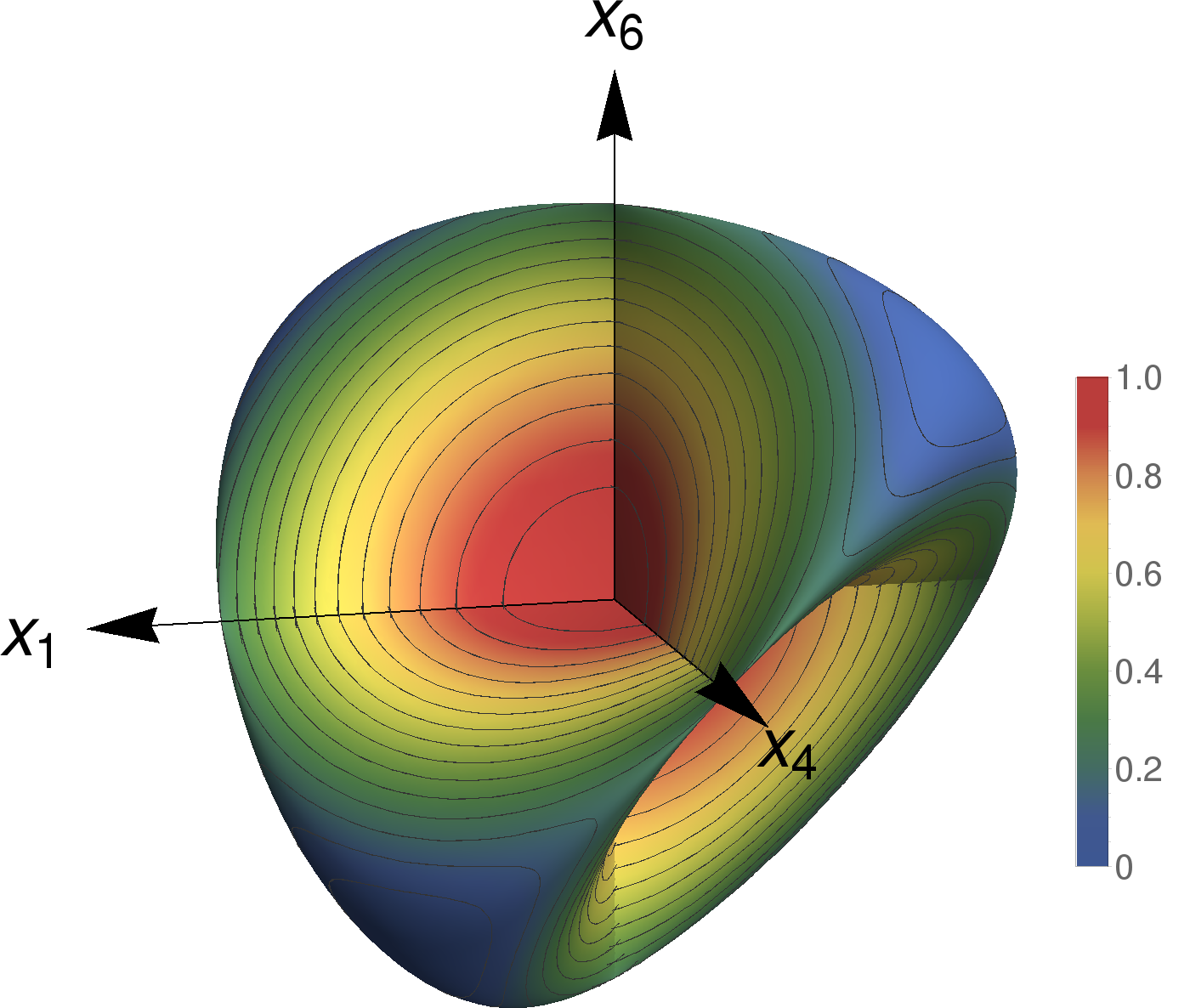
Figure 4.1: A 3-dimensional section of $\Pi(\mathds{C}P^{2})$ through $x_{2}=x_{5}=x_{7}=0$ plane, first printed in [24]. The color indicates the corresponding scaled and shifted dispersion $\bar{\updelta}$, which has its minimum at $0$ ($\triangleq\frac{2}{3+N}$) and maximum at $1$ ($\triangleq\frac{3}{3+N}$). The lines represent contour lines of $\bar{\updelta}$.

The dispersion (4.22) reduces in the limit to

$$\lim_{\varphi_{1},\varphi_{3}\to 0}\updelta(\boldsymbol{\varphi})= \frac{3}{8\,(3+N)}\frac{1}{|\boldsymbol{\varphi}|^{4}}\left\{4\,\varphi_{2}^{2}\,\varphi_{4}^{2}\,\cos|\boldsymbol{\varphi}|\right.$$

$$+ \left.\left(\varphi_{2}^{4}+\varphi_{2}^{2}\,\varphi_{4}^{2}+\varphi_{4}^{4}\right)\cos 2|\boldsymbol{\varphi}|\right.+\left.7\,(\varphi_{2}^{4}+\varphi_{4}^{4})+11\,\varphi_{2}^{2}\,\varphi_{4}^{2}\right\}$$ (4.26)

whose global minima lie at

$$|\varphi_{2}|=|\varphi_{4}|=\sqrt{2}\arctan(\sqrt{2}).$$ (4.27)

This corresponds to 4 points on $\Pi(\mathds{C}P^{2})$, given by

$$c_{N}\frac{N}{3}\begin{pmatrix}-1\\ 0\\ 1\\ 0\\ 1\\ 0\end{pmatrix},\quad c_{N}\frac{N}{3}\begin{pmatrix}1\\ 0\\ 1\\ 0\\ -1\\ 0\end{pmatrix},\quad c_{N}\frac{N}{3}\begin{pmatrix}-1\\ 0\\ -1\\ 0\\ -1\\ 0\end{pmatrix},\quad c_{N}\frac{N}{3}\begin{pmatrix}1\\ 0\\ -1\\ 0\\ 1\\ 0\end{pmatrix},$$

which can be seen in 4.1 as centers of the blue zones.

Limit $\varphi_{3},\varphi_{4}\to 0$.

Another interesting case is the limit $\varphi_{3},\varphi_{4}\to 0$, corresponding to rotations by $T^{4}$ and $T^{5}$. Since $\{T^{4},T^{5},T^{8}\}$ form a $\mathfrak{su}(2)$ subalgebra of $\mathfrak{su}(3)$, this essentially reduces to the squashed fuzzy sphere. Here

$$\lim_{\varphi_{3},\varphi_{4}\to 0}\vec{\bf x}(\boldsymbol{\varphi}) =c_{N}\frac{N}{2}\frac{1}{|\boldsymbol{\varphi}|}\begin{pmatrix}0\\ 0\\ \varphi_{2}\,\sin|\boldsymbol{\varphi}|\\ \varphi_{1}\,\sin|\boldsymbol{\varphi}|\\ 0\\ 0\end{pmatrix},$$ (4.28)

which implies that the image of $\vec{\bf x}$ in this limit is the disk $\mathds{D}_{R}=\{x,y\in\mathds{R},\,x^{2}+y^{2}\leq R^{2}=c_{N}\frac{N}{2}\}$ which is of course simply the ordinary squashed sphere. The dispersion (LABEL:disp_scp2) then reduces to

$$\lim_{\varphi_{3},\varphi_{4}\to 0}\updelta(\boldsymbol{\varphi})= \frac{3}{8\,(3+N)}\left(7+\cos(2|\boldsymbol{\varphi}|)\right).$$ (4.29)

The minima are given by $|\boldsymbol{\varphi}|=\sqrt{\varphi_{1}^{2}+\varphi_{2}^{2}}=\pi/2$, which corresponds to the boundary of the disk $\partial\mathds{D}_{R}$. In 4.2 a picture of the 2-dimensional squashed fuzzy sphere is given indicating the dispersion.

These calculations will be complemented below by a numerical algorithm to determine optimally localized states, which allow to capture the semi-classical limit without relying on any theoretical expectation. This algorithm will not only support the above interpretation for squashed $\mathds{C}P_{N}^{2}$, but is applicable to arbitrary matrix configurations which admit an interpretation in terms of a semi-classical geometry.

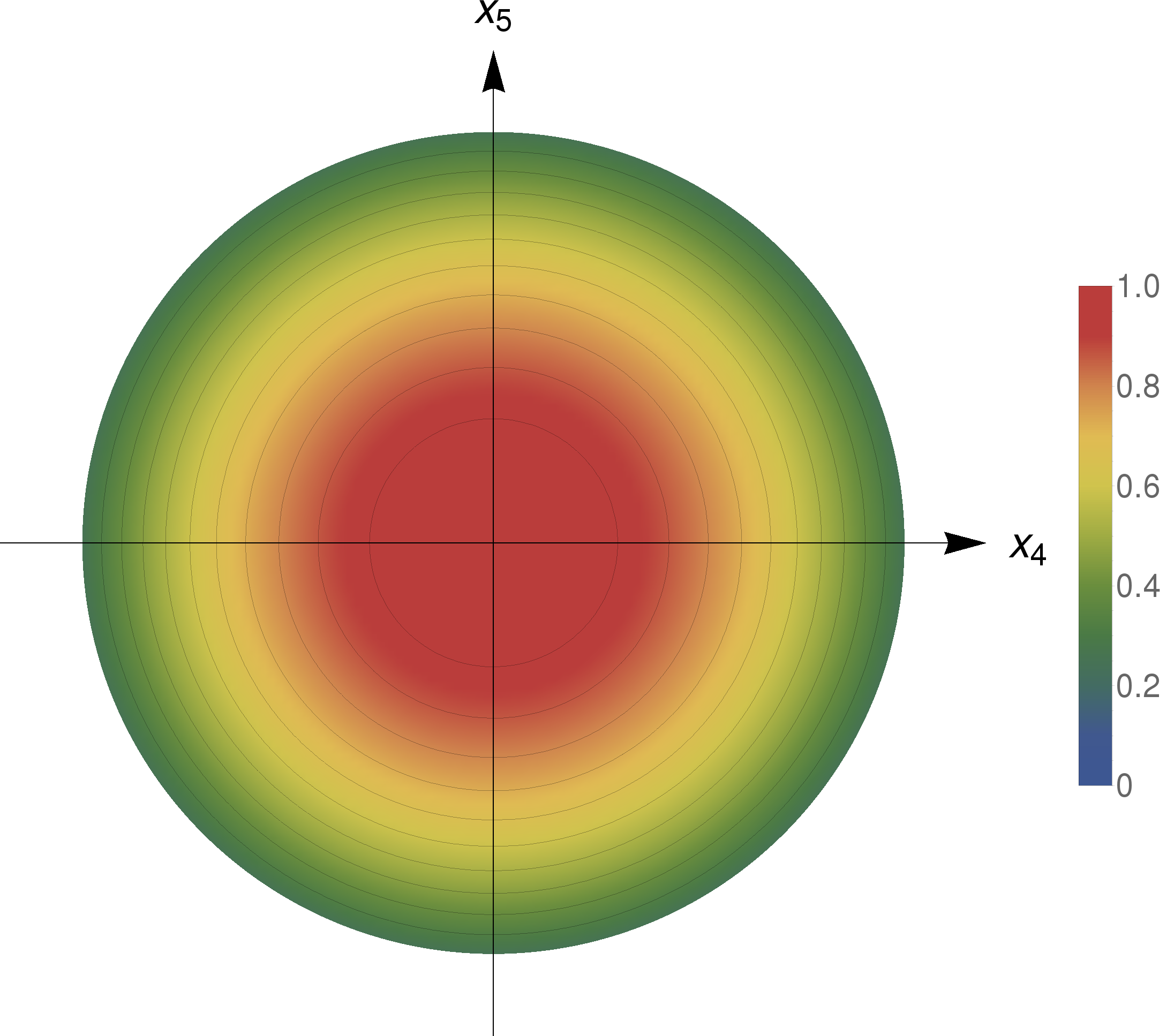
Figure 4.2: Semi-classical limit of the squashed fuzzy sphere. The color indicates the corresponding scaled dispersion $\bar{\updelta}$ which has its minimum at $0$ ($\triangleq\frac{2}{3+N}$) and maximum at $1$ ($\triangleq\frac{3}{3+N}$). The lines represent contour lines of $\bar{\updelta}$.

5 Generalized coherent states

The above definition of Perelomov coherent states is applicable only to very special matrix backgrounds related to Lie groups. Our aim now is to extend the idea of these states to arbitrary matrix configurations, in order to extract some approximate classical geometry from fuzzy spaces described by such matrices.

To this end, we will introduce the concepts of optimal localized states and quasi-coherent states, which are applicable to generic matrix configurations. However, this alone does not quite suffice to extract the classical geometry, since it applies to any point in the embedding space (or target space). Indeed it is clear that not every matrix background will have a geometric interpretation. In section 7 we will then use these quasi-coherent states to single out backgrounds which do define a reasonable approximate geometry, and to to “measure” and characterize this geometry. This will be possible provided the background admits a certain hierarchy, which allows to focus on a suitable subset of quasi-minimal states.

5.1 Optimal localized states and quasi-coherent states

We recall the coherent states on the fuzzy sphere $S^{2}_{N}$: their expectation values $\vec{\bf x}(\Psi_{N})$ are points on a sphere with a certain radius $r_{N}$, and their dispersion is minimal among all states, in particular among all states with the given expectation value. However given some generic matrix background, we do not know a priori any preferred location; this is what we want to extract. Moreover as seen in the example of squashed ${\mathds{C}}P^{2}_{N}$, we should expect that the optimal dispersion of the ”coherent states” depends on the location, as the scale of noncommutativity $|\Theta^{ab}(x)|$ may depend on $x$; hence looking for states with “globally” minimal dispersion is too restrictive. However, what we can do is first fix some point $\vec{x}\in\mathds{R}^{d}$, focus on those states whose expectation value $\vec{\bf x}(\Psi_{N})$ is closest to $\vec{x}$, and choose among those the ones with minimal dispersion. In a next step, the semi-classical location of the matrix background can then be identified as those $\vec{x}\in\mathds{R}^{d}$ where that dispersion is “small”; the latter will be made more precise below, using the concept of a “hierarchy”.

This leads to the following definition of an “optimal localized state”:

Definition 3 (Optimal Localized State).

Let $\vec{x}$ be a point in target space $\mathds{R}^{d}$. A state $\left|\Psi\right\rangle\in\mathscr{H}_{N}$ is called an optimal localized state at $\vec{x}\in\mathds{R}^{d}$, if the following properties hold:

1. The expectation values $\vec{\bf x}(\Psi)$ are optimal, i.e.

   $$\left|\vec{x}-\vec{\bf x}(\Psi)\right|=\min_{\left|\psi\right\rangle\in\mathscr{H}_{N}}\left|\vec{x}-\vec{\bf x}(\psi)\right|.$$ (5.1)

2. Let $\mathscr{L}_{p}\subset\mathscr{H}_{N}$ be the set of states obeying property (1). We demand that the dispersion is minimal with respect to all states in $\mathscr{L}_{p}$, i.e.

   $$\updelta(\Psi)=\min_{\left|\lambda\right\rangle\in\mathscr{L}_{p}}\updelta(\lambda).$$ (5.2)

Since the state space

$$\mathscr{H}_{N}/U(1)\cong{\mathds{C}}P^{M}$$ (5.3)

is compact, the space of optimal localized states is non-empty for each $\vec{x}\in\mathds{R}^{d}$. This definition captures the notion of a state which can be thought of as “the best” approximation of a classical point $\vec{x}\in\mathds{R}^{d}$. However, this definition is rather cumbersome both numerically and analytically. The following alternative definition captures both conditions 1. and 2., but turns out to be much more useful:

Definition 4 (Quasi-coherent states).

Let $\vec{x}$ be a point in target space $\mathds{R}^{d}$. A state $\left|\Psi\right\rangle\in\mathscr{H}_{N}$ is called a quasi-coherent state at $\vec{x}\in\mathds{R}^{d}$, if the following property holds:

$$E(\vec{x}):=\left|\vec{x}-\vec{\bf x}(\Psi)\right|^{2}+\updelta(\Psi)\qquad\mbox{is minimal for given}\ \vec{x}.$$ (5.4)

We will denote $E(\vec{x})$ as displacement energy.

This will be reformulated in terms of an eigenvalue problem in section 6.

To get some insight, consider again the example of the fuzzy sphere $S^{2}_{N}$. Clearly the Perelomov coherent states are both optimally localized and also quasi-coherent states for $\vec{x}=\vec{\bf x}(\psi)$ with $|\vec{x}|=r_{N}$. If we choose $|\vec{x}|>r_{N}$, the corresponding optimally localized state is still a Perelomov state localized at the nearest point $x^{\prime}\in S^{2}_{r_{N}}$. In contrast for $|\vec{x}|<r_{N}$, the states with minimal $\left|\vec{x}-\vec{\bf x}(\Psi)\right|$ are not expected to be the Perelomov states in general, and therefore the optimally localized states will have higher dispersion. Therefore we can choose among all optimally localized states those which have smallest or nearly-smallest dispersion $\updelta$. Their expectation values $\vec{\bf x}(\psi)$ will then reproduce the effective location of $S^{2}$. This can be determined by scanning the state space $\mathscr{H}_{N}/U(1)\cong{\mathds{C}}P^{M}$, as described below.

For the quasi-coherent states, the story is quite different. We will show in section 8.1 that the quasi-coherent states for $S^{2}_{N}$ are always Perelomov states as long as $\vec{x}\neq 0$, located at the point on $S^{2}$ which is closest to $\vec{x}$. In this case, the function $E(\vec{x})$ serves as a measure for the deviation of the quasi-coherent state from $\vec{x}$, and $S^{2}_{r_{N}}$ is recovered as the minimum locus of $E(\vec{x})$. This can be determined by scanning the target space $\mathds{R}^{d}$. Clearly this approach is much more efficient, and will be described in detail in section 7.

Scanning state space.

Let us briefly describe a scanning procedure for optimal localized states. For sufficiently generic matrix backgrounds, we must choose some cutoff $\updelta_{0}$ which selects the near-minimal dispersions $\updelta\leq\updelta_{0}$. Then the (compact) phase space $\mathscr{H}_{N}/U(1)\cong{\mathds{C}}P^{M}$ can be scanned, selecting those states with dispersion $\leq\updelta_{0}$. This is facilitated by equipping ${\mathds{C}}P^{M}$ with the Fubini-Study metric. The selected states $\psi$ with small dispersion will be approximations to the optimally localized states at $\vec{\bf x}(\psi)$, and these expectation values $\vec{\bf x}(\psi)$ define the effective approximate geometry.

Clearly the cutoff $\updelta_{0}$ must be chosen by hand, and there is no global choice of cutoff $\updelta_{0}$ which works for all cases. This is analogous to the process of “focusing” a camera, when trying to take a picture of some object. If the cutoff $\updelta_{0}$ is chosen too small, too few points may be selected; this is easily seen for the fuzzy ellipsoid, where only the two extremal points might survive. On the other hand if $\updelta_{0}$ is chosen too large, we will obtain a very blurred picture.

We implemented this idea numerically, and it turns out to work for simple spaces where a good “hierarchy” exists even for low dimensional matrices. However for more complicated spaces such as squashed $\mathds{C}P^{2}$, the state space becomes very large, requiring an unreasonable computational effort. For this reason, we will present a more efficient procedure in the next section, based on point probes and quasi-coherent states. This is inspired by the ideas of intersecting fuzzy branes and point probes in [12, 11].

6 Point probes and quasi-coherent states

In the present section we develop an efficient approach to optimally localized states, based on the idea of point probes. This can be viewed as a special case of intersecting noncommutative branes discussed in [12], and it was first applied in Berenstein [11] in the present context. Similar ideas are also used by Ishiki in [10] in the large $N$ limit. The idea is to measure the energy of strings connecting the probe with the fuzzy brane, which is minimal at the location $\vec{x}$ of the brane. This energy is defined via certain matrix Laplace of Dirac operators. Quasi-coherent states can then be obtained as ground states of these operators at $\vec{x}$, recovering precisely our previous definition in section 5.

Zero-dimensional (point) brane.

First let us consider the special case of a fuzzy brane defined by $d$ real $1\times 1$ matrices $x^{a}\in Mat_{1}(\mathds{C})\cong\mathds{C},\,a=1,\dots,d$ interpreted as embedding functions of a point in $\mathds{R}^{d}$

$$\vec{x}=(x^{1},\dots,x^{d})\in\mathds{R}^{d}$$ (6.1)

This can also be seen via coherent sates: the elements in this algebra have expectation value $(x^{1},\dots,x^{d})$ and zero dispersion. Hence these numbers $x^{a}$ describe a zero-dimensional point-brane embedded in $\mathds{R}^{d}$.

Stack of branes.

We now return to our original matrix configuration $X^{a}$ which characterizes some fuzzy brane embedded in $\mathds{R}^{d}$ and generates a matrix algebra $\mathscr{A}=Mat_{m}(\mathds{C})$. Adding a second fuzzy brane defined by a set of matrices $Y^{a}$ generating the algebra $\mathscr{B}=Mat_{l}(\mathds{C})$, the two branes in target space $\mathds{R}^{d}$ are described by the direct sum

$$\mbox{$\mathfrak{X}$}^{a}:=X^{a}\oplus Y^{a},\qquad a=1,\dots,d$$ (6.2)

acting on $\mathscr{H}_{m}\oplus\mathscr{H}_{l}$ (see [12]), or explicitly in matrix form

$$\mathfrak{X}^{a}=\begin{pmatrix}X^{a}&0\\ 0&Y^{a}\end{pmatrix},\qquad a=1,\dots,d.$$ (6.3)

They generate the algebra $\mathscr{A}\oplus\mathscr{B}\subset Mat_{m+l}(\mathds{C})$.

This becomes more interesting if we consider not only the algebra $Mat_{m}(\mathds{C})\oplus Mat_{l}(\mathds{C})$ (i.e. matrices in block-diagonal form) but the whole matrix algebra $Mat_{m+l}(\mathds{C})$, including the off-diagonal blocks which are elements of $\mathscr{H}_{m}\otimes\mathscr{H}_{l}^{*}$ respectively $\mathscr{H}_{l}\otimes\mathscr{H}_{m}^{*}$. Since these blocks connect the two branes (which means that the branes “interact” in some way), they can be interpreted as oriented strings connecting the two branes described by the matrices $X^{a}$ and $Y^{a}$.

Point probe.

Now we combine the ideas of the point brane and brane interactions in the following way: Given a fuzzy brane embedded in some target space $\mathds{R}^{d}$ one can place a point brane as a probe at a definite location in this space. Then we are able to measure the energies of the strings connecting the brane and the probe. By varying the position of the probe the energies of the connecting strings will change. In particular, if the brane is not “too fuzzy”, there should be a region in space where the energies are relatively low compared to other regions which then can be regarded as an approximation of the semi-classical limit. This background consisting of a brane described by $X^{a}$ and the point brane at $x^{a}$ is defined by

$$\mathfrak{X}^{a}=\begin{pmatrix}X^{a}&0\\ 0&x^{a}\end{pmatrix},\qquad a=1,\dots,d$$ (6.4)

with $d$ real numbers $x^{a}$.

6.1 Laplace operator

The (matrix) Laplace operator $\boxempty_{\mathfrak{X}}:Mat_{m+1}(\mathds{C})\to Mat_{m+1}(\mathds{C})$ on the above background $\mathfrak{X}^{a}$ is given by

$$\boxempty_{\mathfrak{X}}=\sum_{a=1}^{d}[\mathfrak{X}^{a},[\mathfrak{X}^{a},.]].$$ (6.5)

It acts on the Hilbert space $End(\mathscr{H})=End(\mathscr{H}_{m}\oplus\mathds{C})=End(\mathscr{H}_{m})\oplus\mathscr{H}_{m}\oplus\mathscr{H}_{m}^{T}\oplus\mathds{C}$. It is natural to interpret the two off-diagonal blocks $\mathscr{H}_{m}\oplus\mathscr{H}_{m}^{T}$ as (oriented) strings stretching between the brane described by $X^{a}$ and the point brane at $x^{a}$. We are only interested here in the energies of this string sector, represented by vectors $\Phi\in Mat_{m+1}({\mathds{C}})$ of the form

$$\mbox{$\Phi$}=\begin{pmatrix}\begin{array}[]{ccc}0&\cdots&0\\ \vdots&\ddots&\vdots\\ 0&\cdots&0\end{array}&\left|\phi\right\rangle\\ \left\langle\phi\right|&0\end{pmatrix}\quad\in\mathscr{H}_{m}\oplus\mathscr{H}_{m}^{T}$$ (6.6)

with $\left|\phi\right\rangle\in\mathscr{H}_{m}$. Denoting the restriction of the full matrix Laplacian to $\mathscr{H}_{m}\oplus\mathscr{H}_{m}^{T}$ by $\boxempty_{x}$, this yields

$$\boxempty_{\mathfrak{X}}\Phi = \sum_{a}[\mathfrak{X}^{a},[\mathfrak{X}^{a},\Phi]]=\sum_{a}\left(\mathfrak{X}^{a}\mathfrak{X}^{a}\Phi+\Phi\mathfrak{X}^{a}\mathfrak{X}^{a}-2\mathfrak{X}^{a}\Phi\mathfrak{X}^{a}\right)$$ (6.7)

$$= \begin{pmatrix}\begin{array}[]{ccc}0&\cdots&0\\ \vdots&\ddots&\vdots\\ 0&\cdots&0\end{array}&\sum\limits_{a}(X^{a}-x^{a})^{2}\left|\phi\right\rangle\\ \left\langle\phi\right|\sum\limits_{a}(X^{a}-x^{a})^{2}&0\end{pmatrix}$$

and thus the Laplace operator $\boxempty_{x}$ can be written in terms of

$$\boxempty_{x}=\sum\limits_{a=1}^{d}\left(X^{a}-x^{a}\right)^{2}\$$ (6.8)

acting on $\left|\phi\right\rangle$ and $\left\langle\phi\right|$, respectively.

Let us consider the corresponding quadratic form $\frac{1}{2}\mathrm{tr}(\Phi^{\dagger}\boxempty_{\mathfrak{X}}\Phi)$. It can be written as

$$\frac{1}{2}\mathrm{tr}(\Phi^{\dagger}\boxempty_{\mathfrak{X}}\Phi)=\left\langle\phi\right|\boxempty_{x}\left|\phi\right\rangle =\sum_{a}\left(\Delta_{\phi}X^{a}\right)^{2}+\sum_{a}\left(\left\langle\phi\right|X^{a}\left|\phi\right\rangle-x^{a}\right)^{2}$$

$$=\updelta(\phi)+|\vec{\bf x}(\phi)-\vec{x}|^{2}$$

$$=:E(\vec{x})$$ (6.9)

assuming that $\phi$ is normalized. We will denote this as displacement energy, which coincides with $E(\vec{x})$ in the Definition 4 of quasi-coherent states. In particular, the minimum of $E(\vec{x})$ is precisely the smallest eigenvalue of $\boxempty_{x}$, and the corresponding quasi-coherent state is given by the corresponding eigenvector. We can therefore reformulate the definition (4) of quasi-coherent states as follows:

Definition 5 (Quasi-coherent states II).

Let $\vec{x}$ be a point in target space $\mathds{R}^{d}$. Then the quasi-coherent state(s) at $\vec{x}$ are defined to be the ground state(s) $\Psi$ of $\boxempty_{x}$, and their eigenvalue

$$\boxempty_{x}\Psi=E(\vec{x})\Psi$$ (6.10)

is the displacement energy.

This provides a very efficient and powerful way to obtain quasi-coherent states by solving the eigenvalue problem. It also elucidates the relation with the standard definition in quantum mechanics, interpreting $\boxempty_{x}$ as deformed quantum-mechanical harmonic oscillator centered at $\vec{x}$.

Having solved the problem of finding quasi-coherent states for given $\vec{x}\in\mathds{R}^{d}$, we still have to scan the target space in order to identify the regions with small $E(\vec{x})$; this will be discussed in detail below. In any case, we have reduced the task to a $d$-dimensional problem, independent of the size of the matrices. This is very important, since $N$ should be sufficiently large to obtain a clear hierarchy of energies as discussed below. For example, squashed $\mathds{C}P^{2}$ corresponding to the $SU(3)$-representations $(0,20)$ has a $231$- dimensional state space, while the dimension of the target space in this case is $d=6$.

It is remarkable that these stringy ideas greatly simplify the problem of measuring quantum geometries.

6.2 Dirac operator

Similar ideas also work for the Dirac operator instead of the Laplace operator. The matrix Dirac operator $\not{D}_{\mathfrak{X}}\in End(\mathds{C}^{k}\otimes Mat_{m+1}(\mathds{C}))$, $k=2^{\lfloor\frac{d}{2}\rfloor}$ is defined as

$$\not{D}_{\mathfrak{X}}=\sum_{a=1}^{d}\gamma^{a}\otimes[\mathfrak{X}^{a},.]$$ (6.11)

with $\left\{\gamma^{a},\,a=1,\dots,d\right\}$ forming a representation of the Clifford algebra associated to $\mathds{R}^{d}$. Again we are only interested in the off-diagonal entries of states $\Psi\in\mathds{C}^{k}\otimes Mat_{m+1}(\mathds{C})$ in the presence of a point brane

$$\Psi=\begin{pmatrix}\begin{array}[]{ccc}0&\cdots&0\\ \vdots&\ddots&\vdots\\ 0&\cdots&0\end{array}&\left|\psi\right\rangle\\ \left\langle\psi\right|&0\end{pmatrix}$$ (6.12)

where $\left|\psi\right\rangle\in\mathds{C}^{k}\otimes\mathscr{H}_{m}$ is a spinor-valued state. Then the action of the Dirac operator $\not{D}_{\mathfrak{X}}$ on $\Psi$ is given by

$$\not{D}_{\mathfrak{X}}\Psi = \sum_{a}\gamma^{a}[\mathfrak{X}^{a},\Psi]=\sum_{a}\gamma^{a}(\mathfrak{X}^{a}\Psi-\Psi\mathfrak{X}^{a})$$ (6.13)

$$= \begin{pmatrix}\begin{array}[]{ccc}0&\cdots&0\\ \vdots&\ddots&\vdots\\ 0&\cdots&0\end{array}&\sum\limits_{a}\gamma^{a}(X^{a}-x^{a})\left|\psi\right\rangle\\ \left\langle\psi\right|\sum\limits_{a}\gamma^{a}(X^{a}-x^{a})&0\end{pmatrix}.$$

Restricted to the off-diagonal $\mathds{C}^{k}\otimes\mathscr{H}_{m}$, it reduces to

$$\not{D}_{x}=\sum_{a=1}^{d}\gamma^{a}(X^{a}-x^{a})$$ (6.14)

which is a hermitian operator, with square

$$\not{D}_{x}^{2}=\boxempty_{x}+\Sigma^{ab}[X^{a},X^{b}]$$ (6.15)

where $\Sigma^{ab}:=\frac{1}{4}[\gamma^{a},\gamma^{b}]$. The corresponding quadratic form reads

$$\frac{1}{2}\mathrm{tr}(\Psi^{\dagger}\not{D}_{\mathfrak{X}}^{2}\Psi) =\left\langle\psi\right|\not{D}_{x}^{2}\left|\psi\right\rangle=\left\langle\psi\right|\boxempty_{x}\left|\psi\right\rangle+\sum_{a,b=1}^{d}\left\langle\psi\right|\Sigma^{ab}[X^{a},X^{b}]\left|\psi\right\rangle$$

$$=|\vec{\bf x}(\psi)-\vec{x}|^{2}+\updelta(\psi)+S(\psi),$$ (6.16)

where we define

$$S(\psi) :=\sum_{a,b=1}^{d}\left\langle\psi\right|\Sigma^{ab}[X^{a},X^{b}]\left|\psi\right\rangle$$

$$\vec{\bf x}(\psi) :=\left\langle\psi\right|X^{a}\left|\psi\right\rangle$$ (6.17)

and similarly $\updelta(\psi)$ for spinor-valued states. Since $\not{D}_{x}^{2}$ is positive, we conclude that $\updelta(\psi)+S(\psi)\geq 0$ (because it is independent of $\vec{x}$!), and therefore

$$|\vec{\bf x}(\psi)-\vec{x}|^{2}\leq\left\langle\psi\right|\not{D}_{x}^{2}\left|\psi\right\rangle.$$ (6.18)

Furthermore, the ground state $\left|\psi_{0}\right\rangle$ of $\not{D}_{x}^{2}$ of course satisfies $\left\langle\psi_{0}\right|\not{D}_{x}^{2}\left|\psi_{0}\right\rangle\leq\left\langle\psi\right|\not{D}_{x}^{2}\left|\psi\right\rangle$ for every normalized state $\left|\psi\right\rangle\in{\mathds{C}}^{k}\otimes\mathscr{H}_{m}$. Choosing $\left|\psi\right\rangle=\left|s\right\rangle\otimes\left|\phi\right\rangle$ for some $\left|s\right\rangle\in{\mathds{C}}^{k}$ and for $\left|\phi\right\rangle$ being the ground state of the Laplace operator $\boxempty_{x}$, we have

$$\left\langle\psi_{0}\right|\not{D}_{x}^{2}\left|\psi_{0}\right\rangle\leq E_{L}(\vec{x})+S(s,\phi),$$ (6.19)

where $E_{L}(\vec{x})$ denotes the Laplace displacement energy (6.9). Note that replacing $\left|s\right\rangle\to C\left|s^{*}\right\rangle$ with its charge conjugate yields a sign flip of $S(s,\phi)$. Thus, we can choose $\left|s\right\rangle$ such that $S(s,\phi)$ is negative. We therefore get the following estimate for the groundstate $\left|\psi_{0}\right\rangle$ respectively its eigenvalue:

$$|\vec{\bf x}(\psi_{0})-\vec{x}|^{2}\leq\left\langle\psi_{0}\right|\not{D}_{x}^{2}\left|\psi_{0}\right\rangle\leq E_{L}(\vec{x}).$$ (6.20)

If the ground state happens to be a product state $\left|\psi_{0}\right\rangle=\left|s_{0}\right\rangle\otimes\left|\phi_{0}\right\rangle$, the same arguments provide the estimate

$$|\vec{\bf x}(\psi_{0})-\vec{x}|^{2}\leq\left\langle s_{0},\phi_{0}\right|\not{D}_{x}^{2}\left|s_{0},\phi_{0}\right\rangle\leq|\vec{\bf x}(\psi_{0})-\vec{x}|^{2}+\updelta(\psi_{0}).$$ (6.21)

This leads to the following definition:

Definition 6 (Quasi-coherent spinor states).

Let $\vec{x}$ be a point in target space $\mathds{R}^{d}$. Then the quasi-coherent spinor state(s) at $\vec{x}$ are defined to be the ground state(s) of $\not{D}_{x}^{2}$, and their eigenvalue

$$\not{D}_{x}^{2}\Psi=E(\vec{x})\Psi$$ (6.22)

is the (spinor) displacement energy.

The function $E(\vec{x})$ satisfies the estimate (6.20)

$$|\vec{\bf x}(\psi)-\vec{x}|^{2}\leq E(\vec{x})\leq E_{L}(\vec{x}).$$ (6.23)

It turns out that this $E(\vec{x})$ is very powerful to determine the location of the noncommutative brane: in all cases under consideration, $\not{D}_{x}$ appears to have exact (!) zero modes on the branes. On the other hand, $E(\vec{x})$ does not provide immediate information on the dispersion $\updelta(\Psi)$, hence on the quality of the semi-classical approximation. In the same vein, the ground state(s) $\Psi$ may or may not be product states in $\mathds{C}^{k}\otimes\mathscr{H}_{m}$. This information could be extracted by keeping track of additional information (e.g. the behavior under charge conjugation, possible degeneracies, the dispersion etc.), or simply by taking into account also the Laplace operator. Therefore in the present paper, we will consider both approaches using $\not{D}_{x}$ and $\Box$, and apply the same algorithm in section 7 to extract the location of the brane from quasi-minima of the functions $E(\vec{x})$. This approach applies independently of possible degeneracies of the ground state(s).

7 Measuring the quantum geometry

Having the quasi-coherent states from the lowest eigenvectors of $\boxempty_{x}$ or $\not{D}_{x}^{2}$ at our disposal, we now address the problem of scanning the target space $\mathds{R}^{d}$ to determine a subset $\mathscr{M}_{E}\subset\mathds{R}^{d}$ with quasi-minimal displacement energy $E$, and corresponding quasi-minimal states $\mathscr{S}_{E}\subset\mathds{C}P^{M}$. Their expectation values produce a manifold

$$\mathscr{M}:=\vec{\bf x}(\mathscr{S}_{E})\ \approx\mathscr{M}_{E},$$ (7.1)

which represents the semi-classical limit of the matrix geometry.

7.1 Quasi-minimal energy regions and hierarchy

Assume that we have found (numerically or analytically) the smallest eigenvalue $E(\vec{x})$ of $\boxempty_{x}$ for each $x\in\mathds{R}^{d}$, or the smallest eigenvalue of $\not{D}_{x}^{2}$. This defines the “displacement energy“ function

$$E:\,\mathds{R}^{d} \to\mathds{R}$$ (7.2)

$$\vec{x} \mapsto E(\vec{x})=\min\left({\rm spec}\,\boxempty_{x}\right)$$

for the Laplacian, or similarly

$$E:\,\mathds{R}^{d} \to\mathds{R}$$ (7.3)

$$\vec{x} \mapsto\min\left({\rm spec}\,\not{D}_{x}^{2}\right)$$

for the Dirac operator. Let us focus on the Laplacian for simplicity, and assume that the multiplicity of its lowest eigenspace is one. Then the function $E(\vec{x})=\left|\vec{x}-\vec{\bf x}(\Psi)\right|^{2}+\updelta(\Psi)$ (6.9) can be interpreted as zero point energy of a string stretching from $\vec{x}$ to the fuzzy brane, and thereby encodes its location. $E(\vec{x})$ is differentiable everywhere except on points where the two smallest eigenvalues cross each other; however, we will completely ignore this issue, since for our numerical purpose we will be working with finite differential quotients anyway.

Now assume that the matrix background describes some quantized manifold $\mathscr{M}\subset\mathds{R}^{d}$ of dimension $k<d$. The difficulty in determining $\mathscr{M}$ is that $E(\vec{x})$ is in general not constant on $\mathscr{M}$, hence it is not sufficient to look for minimal surfaces. However, in view of the explicit form (6.9) we expect that $E(\vec{x})$ grows like the square distance in the directions transversal to $\mathscr{M}$, while it should change only slowly in the directions along $\mathscr{M}$. This means that the Hessian

$$H_{\mu\nu}=\nabla_{\mu}\nabla_{\nu}E$$ (7.4)

at $x\in\mathscr{M}$ should have $k$ small eigenvalues which characterize the embedding of $\mathscr{M}\subset\mathds{R}^{d}$, and $d-k$ large eigenvalues of order one. This essential observation will be exploited in the procedure described below.

Quasi-minima of the $E$-function and its hierarchy.

We now describe a scanning procedure which allows to select a set of quasi-minima $\mathscr{M}_{E}$ of $E$, while verifying a manifold-like structure. Again, this is not a universal procedure, and it may require some “focusing” by hand. The quasi-classical nature of $\mathscr{M}_{E}$ is ensured by noting that for each $x\in\mathscr{M}_{E}$ there is a quasi-coherent state $\psi$, which is the corresponding lowest eigenstate of $\boxempty_{x}$ (or $\not{D}_{x}^{2}$). Its expectation value differs from $\vec{x}$ by at most

$$|\vec{\bf x}(\psi)-\vec{x}|\leq E(x)$$ (7.5)

which is small by construction. This subset of quasi-coherent states $\psi$ will be denoted by $\mathscr{S}_{E}$. We could hence consider either $\mathscr{M}_{E}$ or $\mathscr{M}:=\vec{\bf x}(\mathscr{S}_{E})$ as the semi-classical geometry, as long as $E$ is small. However, it turns out that $\mathscr{M}=\vec{\bf x}(\mathscr{S}_{E})$ works much better, because it is remarkably in-sensitive to small perturbations of $\mathscr{M}_{E}$. This will be understood in the example of the fuzzy sphere in section 8.1, where we will show that the states $\mathscr{S}_{E}$ are always Perelomov states on the sphere even if $\mathscr{M}_{E}$ is slightly off.

Now start with a global minimum $x_{0}$ of $E$. The change of the function $E$ in some direction $\varepsilon$ up to second order in $|\varepsilon|$ is given by

$$|E(x_{0})-E(x_{0}+\varepsilon)|=\frac{1}{2}|\varepsilon^{T}H_{x_{0}}\varepsilon|+\mathcal{O}(|\varepsilon|^{3})$$ (7.6)

where $H_{x_{0}}=\nabla\nabla E$ is the Hesse matrix at $x_{0}$. Assuming that the brane has a slowly varying noncommutative structure $|\nabla\nabla\Theta^{\mu\nu}|\ll 1$ (2.1), one should observe a clear hierarchy of “small” and “large” eigenvalues of $H$. Moreover, the eigenvectors corresponding to the small eigenvalues should constitute a basis of the tangent space $T_{x_{0}}\mathscr{M}_{E}$ at $x_{0}$, while the eigenvectors corresponding to the large eigenvalues (of order one) should constitute a basis of the normal space to $\mathscr{M}_{E}$ at $x_{0}$. Hence $x_{0}+\varepsilon$ is approximately an element of $\mathscr{M}$ for $\varepsilon$ being an eigenvector corresponding to a “small” eigenvalue and $|\varepsilon|$ sufficiently small. In particular, the dimension of the manifold $\mathscr{M}$ is obtained as the number $k$ of small eigenvalues of $H$. This characterization of $\mathscr{M}$ is clear-cut as long as there is a clear hierarchy separating the small and the large eigenvalues of $H$.

If $x_{0}$ is not a local minimum of $E$, then the change of $E(x)$ in a direction $\varepsilon$ is given by

$$E(x_{0}+\varepsilon)-E(x_{0})=\varepsilon\cdot\nabla E_{x_{0}}+\frac{1}{2}\varepsilon^{T}H_{x_{0}}\varepsilon+\mathcal{O}(|\varepsilon|^{3})$$ (7.7)

with $\nabla E_{x_{0}}$ denoting the gradient of $E$ at point $x_{0}$. We can separate $\nabla E_{x_{0}}=(\nabla E_{x_{0}})^{\parallel}+(\nabla E_{x_{0}})^{\perp}$ into the tangential and transversal components, as defined by the Hessian. On the quasi-classical manifold $\mathscr{M}$, we expect that $\nabla E$ points in the tangential directions (i.e. in the span of the low eigenvectors of $H$), so that $(\nabla E)^{\perp}\approx 0$. If this is no longer the case, this indicates that we are moving away from $\mathscr{M}$.

This leads to the following strategy:

Given some quasi-minimum $x_{0}\in\mathscr{M}_{E}\subset\mathds{R}^{d}$ of $E$, the Hesse matrix $H=\nabla\nabla E$ at $x_{0}$ should exhibit a clear hierarchy of small and large eigenvalues. 1. We select all small eigenvalues $\lambda_{i}\ll 1$ of $H$. 2. New quasi-minimal points can be obtained as $x_{i}=x_{0}+\varepsilon_{i}$ where $\varepsilon_{i}$ is an eigenvector corresponding to the eigenvalue $\lambda_{i}$ with $\left|\varepsilon_{i}\right|$ being sufficiently small. 3. The points $x_{i}$ are replaced by the expectation values $\vec{\bf x}(\Psi_{x_{i}})$ with $\Psi_{x_{i}}$ being the quasi-coherent state at $x_{i}$. 4. This procedure should be iterated, verifying the hierarchy of $H$ at each step. The collection of these points constitutes our semi-classical approximation $\mathscr{M}:=\vec{\bf x}(\mathscr{S}_{E})$ with $\mathscr{S}_{E}$ being the set of quasi-coherent states corresponding to $\mathscr{M}_{E}$.

This strategy allows to identify a semi-classical approximation for a large class of examples. The procedure is justified as long as there is a clear hierarchy in the eigenvalues of $H$. It needs to be specified by some cutoffs for this hierarchy, and possibly for $E$, $(\nabla E)^{\perp}$ and/or $|\nabla E|$. Since the hierarchy of eigenvalues depends on the example under consideration, there is no universal prescription; the appropriate parameters must be adjusted for each example individually. This can be compared to taking a picture with a camera, where the photographer needs to adjust the focus to get a sharp image.

Clearly the same procedure applies for the (squared) Dirac operator instead of the Laplace operator. It is an interesting question whether the states selected by the Dirac operator yield the same manifold as the Laplacian. We will provide some numerical and analytical examples in sections 8.1 and 8.3, and we will see that this is the case in simple examples, but not always.

If there is no clear hierarchy of eigenvalues of $H$, the matrices simply do not contain enough information to extract a meaningful semi-classical manifold.

7.2 Numerical procedure

The considerations in the previous section provide the basis for an algorithm to rasterize the manifold $\mathscr{M}\approx\mathscr{M}_{E}$. Locally we can find the tangent space $T_{x_{0}}\mathscr{M}_{E}$ by using algorithm 1, written as so-called pseudo-code.

1:function GetDirections(function $f$, point $x_{0}$, dimension $k$)

2:     $H$ $\leftarrow$ HesseMatrix($x_{0}$) $\triangleright$ Calculate Hesse Matrix $H_{x_{0}}$ at point $x_{0}$.

3:     $\{(\lambda,\varepsilon)\}$ $\leftarrow$ Diag(H) $\triangleright$ Diagonalize $H_{x_{0}}$ with eigenvectors $\varepsilon$ corresponding to eigenvalues $\lambda$.

4:return Select($\{(\lambda,\varepsilon)\}$,$k$) $\triangleright$ Return eigenvectors corresponding to the choice of $k$ “small” eigenvalues.

5:end function

Algorithm 1 Select directions corresponding to a “small” change in $f$

On each point obtained by $x=x_{0}+\varepsilon$ as explained above, we can subsequently apply algorithm 1, identify new tangential directions, and gather new points of $\mathscr{M}_{E}$ respectively $\mathscr{M}$. These will sample an open neighborhood $U_{|\varepsilon|}(x)\subset\mathscr{M}$ for each point $x$, and by repeating this procedure the entire manifold should be covered. If this is done blindly, then many areas will be covered more than once. To avoid this redundancy, one can attempt a nearest neighborhood search [35] with respect to the Euclidean metric, to prevent accepting points which are already covered.

One also has to implement some stopping mechanism which prevents points to be accepted when the above criteria for $\mathscr{M}_{E}$ respective $\mathscr{M}$ are no longer satisfied. A local stop can be imposed if

• $E$ exceeds a certain value $E_{\mathrm{crit}}$,

• the norm of the gradient $|\nabla E|$ or of $(\nabla E)^{\perp}$ exceeds a certain value $\left(\nabla E\right)_{\mathrm{crit}}$,

• the hierarchy of eigenvalues of the Hessian matrix $H_{x}$ no longer holds, i.e. the highest “small” eigenvalue $\lambda$ exceeds a certain value $\lambda_{\mathrm{crit}}$.

A simple unoptimized form of an algorithm which provides a complete point cloud of $\mathscr{M}$ is presented by algorithm 2 where standard programming structures are used.

1:function Rasterize(function $f$, startpoint $x_{0}$, dimension $k$)

2:     $pc\leftarrow List$ $\triangleright$ List of points which constitute the point cloud.

3:     $q\leftarrow Queue$ $\triangleright$ FIFO Queue which holds new unchecked points.

4:

5:     add point $x_{0}$ to $pc$

6:     add point $x_{0}$ to $q$

7:

8:     while $q$ not empty do

9:

10:         $x\leftarrow$ take next element from $q$ $\triangleright$ Current point to process.

11:         $\mathrm{dirs}\leftarrow$ GetDirections($f$,$x$,$k$)

12:

13:         for all directions $\varepsilon$ in $\mathrm{dirs}$ do

14:              project $x_{\mathrm{new}}=x+\varepsilon$ to its corresponding expectation value $\bf{x}_{\mathrm{new}}$

15:              if IsLegal($\bf{x}_{\mathrm{new}}$) is true then $\triangleright$ This refers to the considerations above.

16:                  add $\bf{x}_{\mathrm{new}}$ to $pc$

17:                  add $\bf{x}_{\mathrm{new}}$ to $q$

18:              end if

19:         end for

20:

21:     end while

22:

23:return $pc$

24:end function

Algorithm 2 Successively apply alg. 1 to gather a complete point cloud of $\mathscr{M}$.

Furthermore, we clearly have to restrict the search to a compact subset of $\mathds{R}^{d}$. For compact manifolds $\mathscr{M}$ described by finite-dimensional matrices, these bounds can be easily extracted from the spectrum of $X^{a}$. The result is a point cloud which is an approximation of $\mathscr{M}=\vec{\bf x}(\mathscr{S}_{E})$. The quality of the approximation depends on three aspects. Obviously it is determined by the step length $|\varepsilon|$. Furthermore, the separation of the hierarchy plays an important role, and depends on the dimension of the given $M\times M$ matrices. Finally, the approximation is affected by the above mentioned cut-off parameters $E_{\mathrm{crit}}$, $\left(\nabla E\right)_{\mathrm{crit}}$ or $\lambda_{\mathrm{crit}}$.

7.3 Exact zero modes and brane location from $\not{D}_{x}$

Even though the approach using $\boxempty_{x}$ is conceptually simpler at first sight, it turns out that the Dirac operator $\not{D}_{x}$ has typically better properties. In fact for 2-dimensional fuzzy spaces embedded in $\mathds{R}^{3}$, the quasi-classical manifold $\mathscr{M}$ can be obtained from exact zero modes of $\not{D}_{x}$, as shown by Berenstein [11]. The corresponding exact zero modes of $\not{D}_{x}$ deserve the name coherent (spinor) states. Because the argument is so beautiful we shall repeat it here. One defines the index of $\not{D}_{x}$ as difference of positive and negative eigenvalues,

$${\rm ind}(\not{D}_{x})=\frac{1}{2}(n_{+}-n_{-})$$ (7.8)

Clearly this index is locally constant and can only jump by $\pm 1$ at locations $\vec{x}$ where $\not{D}_{x}$ has a zero mode. It is easy to see that for $\vec{x}\to\infty$ this index always vanishes, ${\rm ind}(\not{D}_{\infty})=0$, while for $\vec{x}=0$ it is one for a fuzzy sphere background (and a large class of deformations thereof). This implies that ${\rm ind}(\not{D}_{x})=0$ defines a surface around the origin, which is the location of the fuzzy sphere.

This argument is very compelling, and our numerical studies (see section 8) indicate that $\not{D}_{x}$ has exact zero modes also for many higher-dimensional fuzzy spaces including the fuzzy torus and squashed fuzzy $\mathds{C}P^{2}$, even if there is no well-defined notion of “interior” and “exterior” space. We can provide a heuristic argument why this is the case. Consider the case of a flat $2n$-dimensional quantum plane $\mathds{R}^{2n}_{\theta}$ with commutation relations $[X^{a},X^{b}]=i\Theta^{ab}\mathds{1}$, embedded in target space $\mathds{R}^{2n+1}$ at the $x^{2n+1}=0$ hyperplane. It is then easy to see (cf. [12, 37]) that the minimal eigenvalue $\lambda^{(2n+1)}(\vec{x})$ of the point probe Dirac operator $\not{D}_{x}^{(2n+1)}$ for a test-brane at $x^{2n+1}\neq 0$ is given by the transversal distance, $\lambda^{(2n+1)}(\vec{x})=x^{2n+1}$, with sign set by the orientation form $\omega^{\wedge n}$ on the quantum plane. This function divides target space $\mathds{R}^{2n+1}$ into “left” and “right” half-spaces defined by $\lambda^{(2n+1)}(\vec{x})>0$ and $\lambda^{(2n+1)}(\vec{x})<0$, respectively. Moreover, the corresponding minimal energy state is a product state $\left|s,\psi\right\rangle=\left|s\right\rangle\otimes\left|\psi\right\rangle$ of a coherent state on $\mathds{R}^{2n}_{\theta}$ and a spinor with definite chirality.

Now consider the generic case of a quantized symplectic space $\mathscr{M}^{2n}\hookrightarrow{\mathds{R}}^{d}$ with $d>2n$, and a point probe brane at $\vec{x}\in\mathds{R}^{d}$. Assume that $\mathscr{M}$ is sufficiently flat near $\vec{x}$, and denote with $\vec{x}_{0}$ the closest point on $\mathscr{M}$ to $\vec{x}$. Then $\mathscr{M}$ can be well approximated by a quantum plane $\mathds{R}^{2n}_{\theta}$ through the tangent space $T_{x_{0}}\mathscr{M}$, and we can consider the reduced $2n+1$-dimensional Dirac operator $\not{D}_{x}^{(2n+1)}$ in the reduced target space $T_{x_{0}}\mathscr{M}\oplus\mathds{R}(\vec{x}-\vec{x}_{0})$, with transversal coordinate $x^{2n+1}$. According to the above discussion, that Dirac operator has a minimal energy state with eigenvalue $\lambda^{(2n+1)}(\vec{x})\sim x^{2n+1}$. Now the full Dirac operator $\not{D}_{x}$ can be considered as a small perturbation of $\not{D}_{x}^{2n+1}\otimes\Gamma_{k}$ with $\Gamma_{k}^{2}=\mathds{1}$. Standard arguments in perturbation theory then imply that $\not{D}_{x}$ has $k$ zero modes going from positive to negative $x^{2n+1}$, provided the perturbation is sufficiently small. Here $k\geq 2$ in the case of several transversal dimensions.

This argument already suggests that in the case of several transversal dimensions $d-2n>1$, one should in general not expect that the zero modes of $\not{D}_{x}$ coincide on some lower-dimensional manifold. In some cases of interest, $\not{D}_{x}$ might not even have any exact zero modes. Our general method as explained above does not require the existence of exact zero modes, and it provides more information which allows to measure the quality of the semi-classical approximation, its effective dimension as well as the dispersion.

The localization properties of these coherent spinor states on 2-dimensional surfaces were studied in [38].

8 Applications and examples

We elaborate the above results and apply the numerical scanning algorithm for several examples, starting with the fuzzy sphere.

8.1 Fuzzy sphere revisited

We recall the fuzzy sphere $S^{2}_{N}$, which is defined by the three matrices $X^{a},\,a=1,\dots,3$ which satisfy the commutation relations

$$[X^{a},X^{b}]=i\,\frac{2}{\sqrt{N^{2}-1}}\,\varepsilon_{abc}X^{c}.$$ (8.1)

8.1.1 The point probe Laplacian $\boxempty_{x}$

For the simple case of the fuzzy sphere we can explicitly evaluate the function $E(\vec{x})$  (7.2) exactly, i.e. the minimal eigenvalue of the point probe Laplacian

$$\boxempty_{x}=\sum_{a=1}^{3}\left(X^{a}-x^{a}\right)^{2}=\mathds{1}-2\sum_{a=1}^{3}x^{a}X^{a}+\sum_{a=1}^{3}x^{a}x^{a}.$$ (8.2)

Since this expression is invariant under $SO(3)$-rotations, it suffices to consider the operator at the north pole $\vec{x}=(0,0,x^{3})$ where

$$\boxempty_{x}=\mathds{1}+|\vec{x}|^{2}-2|\vec{x}|\,X^{3}$$ (8.3)

assuming $x^{3}>0$ to be specific. Obviously, eigenvectors of the operator $\boxempty_{x}$ are eigenvectors of $X^{3}$ and vice versa. Since the eigenvalues of $X^{3}$ are smaller than one, it follows that the smallest eigenvalue $E$ of $\boxempty_{x}$ arises for the highest state vectors $\left|\frac{N-1}{2},\frac{N-1}{2}\right\rangle$. Using $X^{3}\left|\frac{N-1}{2},\frac{N-1}{2}\right\rangle=\sqrt{\frac{N-1}{N+1}}\left|\frac{N-1}{2},\frac{N-1}{2}\right\rangle$, we obtain

$$E(\vec{x})=1+|\vec{x}|^{2}-2|\vec{x}|\sqrt{\frac{N-1}{N+1}}$$ (8.4)

whose minima are given by $|\vec{x}_{\min}|=\sqrt{\frac{N-1}{N+1}}=1+\mathcal{O}(\frac{1}{N})$. Hence the quasi-minimal space $\mathscr{M}_{E}$ is sharply defined by

$$\mathscr{M}_{E}=\{\vec{x}\in\mathds{R}^{3}:\,|\vec{x}|=\sqrt{\frac{N-1}{N+1}}=1+\mathcal{O}(\frac{1}{N})\}.$$ (8.5)

It is remarkable that the quasi-coherent states $\mathscr{S}$ as defined by the point probe Laplacian always coincide with the Perelomov coherent states on $S^{2}_{N}$, even if $\vec{x}$ has the wrong length. Therefore the minimal energy manifold coincides precisely with the expectation values of the coherent states $\mathscr{M}_{E}=\vec{\bf x}(\mathscr{S})$, and minimizes the dispersion $\updelta(\Psi)=\sum_{a=1}^{3}(\Delta_{\Psi}X^{a})^{2}$.

A test of the numerical procedure.

Independent of the above exact computations we check the implementation of the numerical algorithm in this well understood case. As input we take three $10\times 10$ matrices $X^{1},\,X^{2},\,X^{3}$ given by the rescaled generators of $SU(2)$ with the correct normalization factor as in  (LABEL:fuzzysphere_emb_2). They are explicitly given by

$$X^{1} =\frac{2}{\sqrt{99}}\times\mathrm{diag}_{2}\left(\frac{3}{2},2,\frac{\sqrt{21}}{2},\sqrt{6},\frac{5}{2},\sqrt{6},\frac{\sqrt{21}}{2},2,\frac{3}{2}\right)+\mathrm{h.c.},$$

$$X^{2} =-\frac{2\,i}{\sqrt{99}}\times\mathrm{diag}_{2}\left(\frac{3}{2},2,\frac{\sqrt{21}}{2},\sqrt{6},\frac{5}{2},\sqrt{6},\frac{\sqrt{21}}{2},2,\frac{3}{2}\right)+\mathrm{h.c.},$$

$$X^{3} =\mathrm{\frac{2}{\sqrt{99}}\times diag}\left(\frac{9}{2},\frac{7}{2},\frac{5}{2},\frac{3}{2},\frac{1}{2},-\frac{1}{2},-\frac{3}{2},-\frac{5}{2},-\frac{7}{2},-\frac{9}{2}\right)$$ (8.6)

where $\mathrm{diag_{2}}(\dots)$ represents a matrix with entries in the second diagonal.

The numerical procedure then picks a global minimum $\vec{x}_{\min}$ of $E$, with corresponding displacement energy

$$E(\vec{x}_{\min})\approx 0.181818$$

which is in perfect agreement with the theoretical minimum $1-\frac{N-1}{N+1}=1-\frac{9}{11}\approx 0.181818$ and the norm $|\vec{x}_{\min}|=\sqrt{\frac{N-1}{N+1}}\approx 0.904534$. The moduli of the eigenvalues of the Hesse matrix at this point $\vec{x}_{\min}$ are given by $\approx(1.1\times 10^{-6},\,2.4\times 10^{-6},\,2.)$, which exhibits a clear hierarchy. Obviously, two directions are classified as “small”, so that the effective dimension is found to be $\dim\mathscr{M}_{E}=2$.

After applying algorithm 2 the result is a point cloud representing the manifold $\mathscr{M}_{E}$. Under the assumption that the point cloud constitutes a two-dimensional manifold, one can build a mesh of polygons connecting these points to create a visualization of $\mathscr{M}_{E}$. A picture is shown in 8.1. As expected one recovers the sphere $S^{2}$ with radius $R=\sqrt{\frac{N-1}{N+1}}$ to a good approximation.

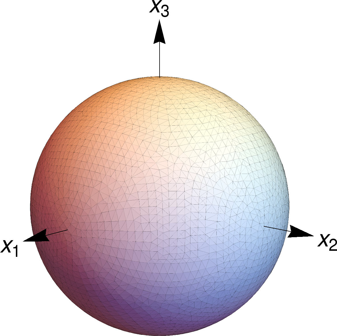
(a) Full picture of $\mathscr{M}=S^{2}_{10}$.

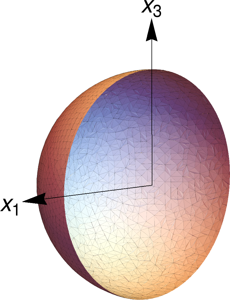
(b) A cut through the $x_{1}-x_{3}$-plane to show that there are no points inside.

Figure 8.1: Visualization of the semi-classical limit of the fuzzy sphere $S_{N}^{2}$ constructed from $S_{10}^{2}$.

8.1.2 The point probe Dirac operator $\not{D}_{x}$

Similar considerations are possible for the Dirac operator

$$\not{D}_{x}=\sum_{a=1}^{3}\sigma^{a}\left(X^{a}-x^{a}\right)$$ (8.7)

with $\sigma^{a}$ being the Pauli matrices

$$\sigma^{1}=\begin{pmatrix}0&1\\ 1&0\end{pmatrix},\qquad\sigma^{2}=\begin{pmatrix}0&-i\\ i&0\end{pmatrix},\qquad\sigma^{3}=\begin{pmatrix}1&0\\ 0&1\end{pmatrix}.$$ (8.8)

Again due to the $SU(2)$ symmetry it is enough to consider points $\vec{x}=(0,0,x^{3})$ on the positive $x^{3}$ axis, so that

$$\not{D}_{x}=\sum_{a=1}^{3}\sigma^{a}X^{a}-\sigma^{3}|\vec{x}|\ .$$ (8.9)

The eigenvector with minimal (absolute) eigenvalue $\left(\sqrt{\frac{N-1}{N+1}}-\left|\vec{x}\right|\right)$ is given by $\left|\uparrow\right\rangle\otimes\left|\frac{N-1}{2},\frac{N-1}{2}\right\rangle$. Thus the minimal energy function $E$ with respect to the squared Dirac operator $\not{D}_{x}^{2}$ is given by

$$E(\vec{x})=\Big{(}\sqrt{\frac{N-1}{N+1}}-|\vec{x}|\Big{)}^{2}.$$ (8.10)

Its minima (which at the same time are roots of $E$) are obviously given by $|\vec{x}_{\min}|=\sqrt{\frac{N-1}{N+1}}$ as in the Laplacian case, which means that we get the same result for the semi-classical limit $\mathscr{M}_{E}$

$$\mathscr{M}_{E}=\{\vec{x}\in\mathds{R}^{3}:\,|\vec{x}|=\sqrt{\frac{N-1}{N+1}}=1+\mathcal{O}(\frac{1}{N})\}.$$ (8.11)

Remarkably, $\not{D}_{x}$ has exact zero modes for $\vec{x}\in\mathscr{M}_{E}\cong S^{2}$, which was first observed in [11] and explained on topological grounds. This interesting phenomenon generalizes to many higher-dimensional cases, including $S^{4}_{N}$ [37, 27] and even squashed ${\mathds{C}}P^{2}$ as discussed below.

We have seen that for the fuzzy sphere, the definition of the coherent states with respect to the Laplacian $\boxempty_{x}$ is essentially equivalent to the definition with respect to the Dirac operator $\not{D}_{x}$. Nevertheless, in a numerical context the method using the Dirac operator has advantages, due to the fact that the minima of $f$ are typically exact roots for all $N$. This leads to a greatly improved precision and hierarchy for small $N$, and quasi- coherent states can be clearly identified even for small $N$. However, we will use the same $10\times 10$ matrices in (8.6) to compare the numerical results with the bosonic approach.

Numerical test.

For the Dirac case our numerical implementation finds a global minimum with

$$E(\vec{x}_{\min})\approx 0,$$

within numerical accuracy. The eigenvalue moduli of the numerical Hesse matrix at point $\vec{x}_{\min}$ are given by $\approx(2.3\times 10^{-6},\,7.3\times 10^{-6},\,2.0)$.

The visual result is the same as in the Laplacian case and is not displayed again.

8.2 Fuzzy torus revisited

Recall, the fuzzy torus $T_{N}^{2}$ is defined by the quantized embedding functions $X^{a}\sim x^{a}$ given by four $N\times N$ matrices

$$X^{1} =(U+U^{\dagger})/2$$ (8.12)

$$X^{2} =-i\,(U-U^{\dagger})/2$$

$$X^{3} =(V+V^{\dagger})/2$$

$$X^{4} =-i\,(V-V^{\dagger})/2$$

with $U$ and $V$ being the shift and clock matrix,

$$U=\begin{pmatrix}0&1\\ &0&1\\ &&\ddots&\ddots\\ &&&0&1\\ 1&&&&0\end{pmatrix},\qquad V=\begin{pmatrix}1\\ &q\\ &&q^{2}\\ &&&\ddots\\ &&&&q^{N-1}\end{pmatrix},$$ (8.13)

and $q=e^{2\pi i/N}$.

8.2.1 The point probe Laplacian $\boxempty_{x}$

The Laplace operator $\boxempty_{x}$ is then defined as

$$\boxempty_{x} =\sum_{a=1}^{4}\left(X^{a}-x^{a}\right)^{2}=\mathds{1}+|\vec{x}|^{2}-2\sum_{a=1}^{4}X^{a}x^{a}$$

$$=\mathds{1}+|\vec{x}|^{2}-U\left(x^{1}-ix^{2}\right)-U^{\dagger}\left(x^{1}+ix^{2}\right)-V\left(x^{3}-ix^{4}\right)-V^{\dagger}\left(x^{3}+ix^{4}\right).$$ (8.14)

In this case we will skip an exact treatment – although possible (cf. [10]) – and turn directly towards the numerical results. To visualize the resulting point cloud which represents a two-dimensional manifold embedded in $\mathscr{M}\subset S^{3}\subset\mathds{R}^{4}$, one can use a generalized stereographic projection $\mathcal{P}:S^{3}\to\bar{\mathds{R}}^{3}$ defined by

$$\mathcal{P}:S^{3}\subset\mathds{R}^{4} \to\bar{\mathds{R}}^{3}$$ (8.15)

$$\begin{pmatrix}x_{1}\\ x_{2}\\ x_{3}\\ x_{4}\end{pmatrix} \mapsto\frac{1}{1-x_{4}}\begin{pmatrix}x_{1}\\ x_{2}\\ x_{3}\end{pmatrix}.$$

The result $\mathcal{P}(\mathscr{M})$ is a two-dimensional manifold embedded in $\mathds{R}^{3}$ which is shown in 8.2.

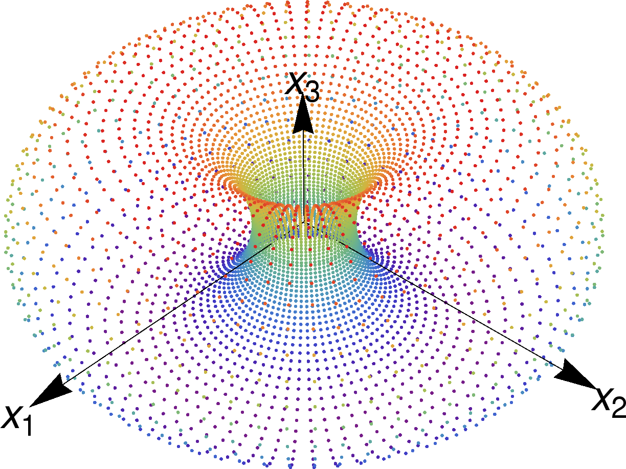
(a) The raw point cloud which is generated by the numerical procedure.

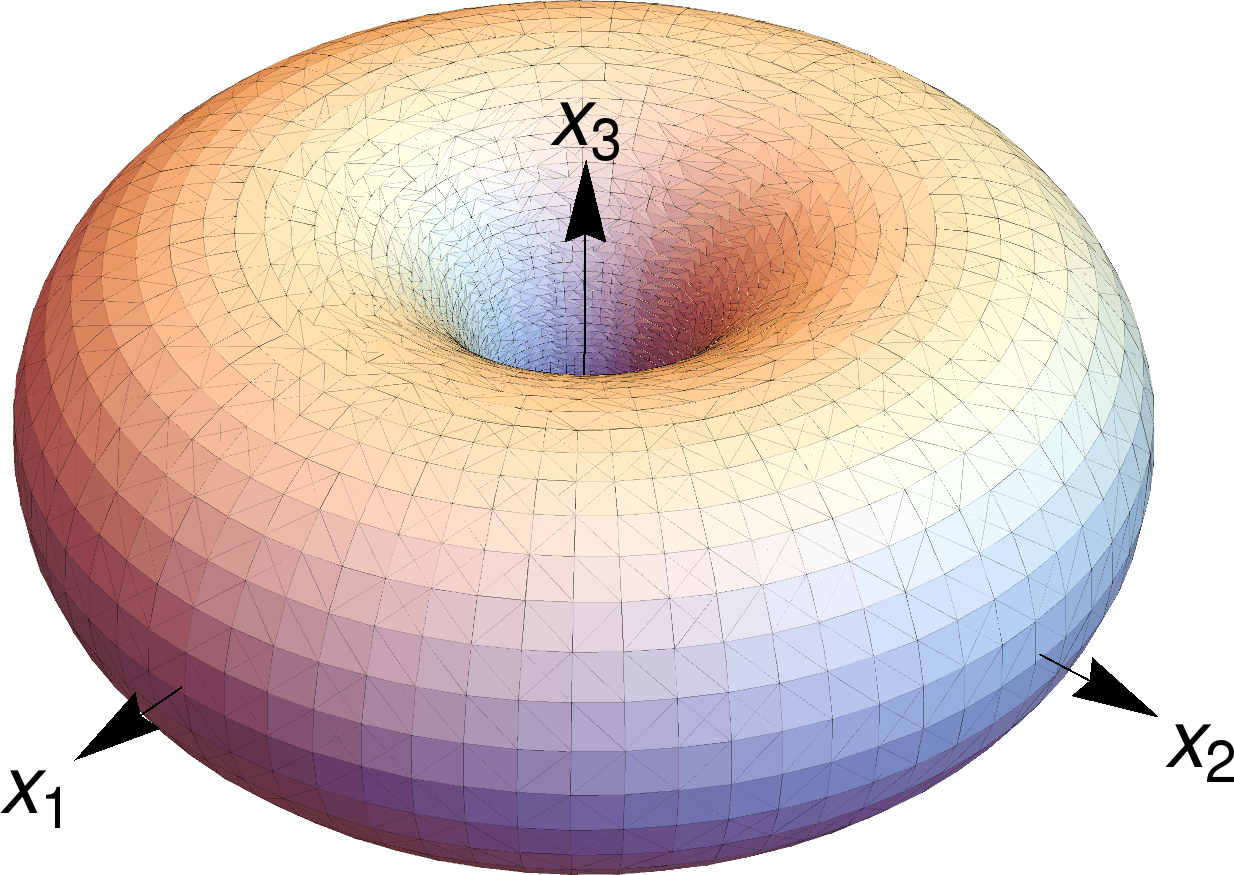
(b) A polygon mesh generated from the point cloud in 8.2a.

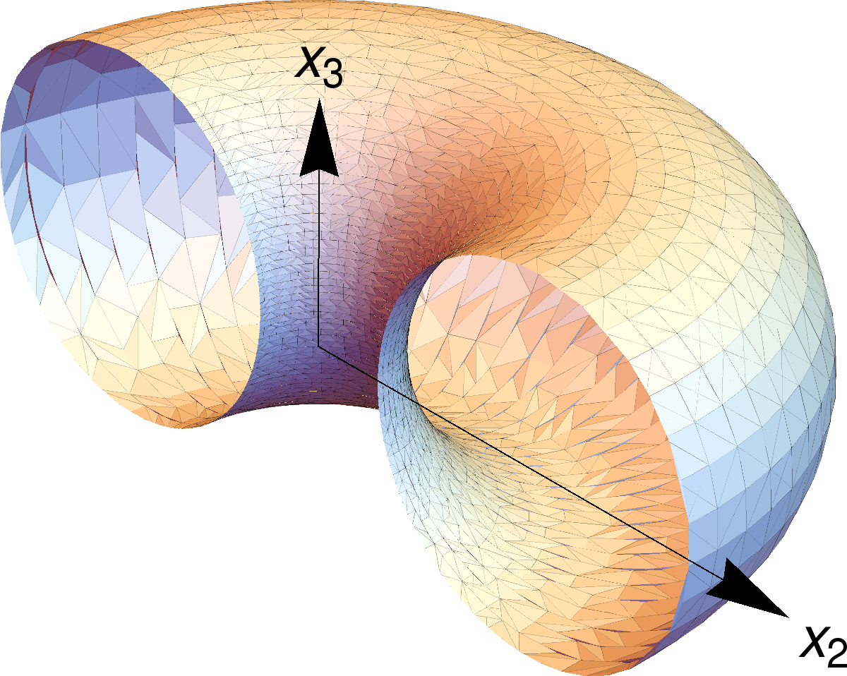
(c) A cut through the torus to show that it is hollow.

Figure 8.2: Visualization of the semi-classical limit of the fuzzy torus $T_{N}^{2}$ constructed from $T_{20}^{2}$.

8.2.2 The point probe Dirac operator $\not{D}_{x}$

The Dirac operator $\not{D}_{x}$ is given by

$$\not{D}_{x}=\sum_{a=1}^{4}\gamma^{a}\left(X^{a}-x^{a}\right)$$ (8.16)

where the following matrices can be used as representation for the Clifford algebra $C\ell_{4}(\mathds{R})$:

$$\gamma^{1} =\left(\begin{array}[]{cccc}0&0&1&0\\ 0&0&0&1\\ 1&0&0&0\\ 0&1&0&0\end{array}\right), \gamma^{2}=\left(\begin{array}[]{cccc}0&0&-i&0\\ 0&0&0&-i\\ i&0&0&0\\ 0&i&0&0\end{array}\right),$$ (8.25)

$$\gamma^{3} =\left(\begin{array}[]{cccc}0&1&0&0\\ 1&0&0&0\\ 0&0&0&-1\\ 0&0&-1&0\end{array}\right),\qquad \gamma^{4}=\left(\begin{array}[]{cccc}0&-i&0&0\\ i&0&0&0\\ 0&0&0&i\\ 0&0&-i&0\end{array}\right).$$ (8.34)

The numerical procedure yields the same point cloud as in 8.2a. Remarkably, even for low dimensional matrices the hierarchy of the Hessian is clearly visible. For $5\times 5$ matrices the Hesse matrix eigenvalues at the determined minimum are $(1.6\times 10^{-5},\,3.5\times 10^{-4},\,1.26,\,1.86)$. The numerically obtained points fulfill

$$E(\vec{x})<8.6\times 10^{-14}$$

which suggests that the Dirac operator $\not{D}_{x}$ has exact zero modes at $T^{2}\subset\mathds{R}^{4}$.

8.3 Squashed $\mathds{C}P_{N}^{2}$ revisited

Now let us turn to squashed fuzzy $\mathds{C}P^{2}$ given by six matrices $X^{a}\sim x^{a},\,a\in\mathcal{I}=\{1,2,4,5,6,7\}$ as explained in section 3.3.

8.3.1 The point probe Laplacian $\boxempty_{x}$

The point probe Laplacian $\boxempty_{x}$ is as always given by

$$\boxempty_{x}=\sum_{a\in\mathcal{I}}\left(X^{a}-x^{a}\right)^{2}.$$ (8.35)

To visualize the numerical result, one can consider the intersection with a 3-dimensional subspace of the target space $\mathds{R}^{6}$. An interesting choice is to consider the limit $x^{2}=x^{5}=x^{7}\to 0$ which can be achieved by simply setting $x^{2}=x^{5}=x^{7}=0$ in (LABEL:scp2_laplc). This corresponds to the limit considered in 4.4. Taking $N=30$, i.e. the representation $(0,30)$, one finds a global minimum at

$$\vec{x}_{\min}\approx\left(0.546391,\,-0.546396,\,0.546392\right)$$

with corresponding energy

$$E(\vec{x}_{\min})\approx 0.052891.$$

The expectation values $\vec{\bf x}(\phi)$ of the coherent state $\phi$ corresponding to this minimum agree with $\vec{x}_{\min}$ for at least $6$ decimal digits. Hence $E(\vec{x}_{\min})\approx\updelta(\phi)$ to a very good approximation.

In 4.4 the Perelomov states were studied and led to a minimal energy value

$$E_{\min}^{\mathrm{th}}=\frac{2}{3+N}\stackrel{{\scriptstyle N=30}}{{\approx}}0.0606061$$

which implies a relative deviation of $\approx 15\%$ from the numerical value. The predicted norm of the expectation values $|\vec{\bf x}(\phi)|$ is

$$|\vec{\bf x}(\phi)|=\sqrt{3}c_{N}N\stackrel{{\scriptstyle N=30}}{{\approx}}0.953463$$

which deviates by $0.7\%$ from the numerically obtained norm.

This numerical evidence suggests that the coherent states for squashed $\mathds{C}P^{2}_{n}$ obtained from $\boxempty_{x}$ are not exactly the Perelomov coherent states but even better ones, if one takes the dispersion $\updelta(\phi)$ as a measure for quality. Nevertheless, the deviations of the expectation values are small, therefore the Perelomov states should suffice as a useful approximation. This can also be seen in 8.3a which approximately looks like 4.1 in 4.4.

8.3.2 The point probe Dirac operator $\not{D}_{x}$ and exact zero modes.

It remains to examine the Dirac operator $\not{D}_{x}$ which in this case is defined as

$$\not{D}_{x}=\sum_{a\in\mathcal{I}}\gamma^{a}\left(X^{a}-x^{a}\right)$$ (8.36)

with the six gamma matrices $\gamma^{a}$ given by

$$\gamma^{1} =\left(\begin{array}[]{cccccccc}0&0&0&0&1&0&0&0\\ 0&0&0&0&0&1&0&0\\ 0&0&0&0&0&0&1&0\\ 0&0&0&0&0&0&0&1\\ 1&0&0&0&0&0&0&0\\ 0&1&0&0&0&0&0&0\\ 0&0&1&0&0&0&0&0\\ 0&0&0&1&0&0&0&0\end{array}\right), \gamma^{2} =\left(\begin{array}[]{cccccccc}0&0&0&0&-i&0&0&0\\ 0&0&0&0&0&-i&0&0\\ 0&0&0&0&0&0&-i&0\\ 0&0&0&0&0&0&0&-i\\ i&0&0&0&0&0&0&0\\ 0&i&0&0&0&0&0&0\\ 0&0&i&0&0&0&0&0\\ 0&0&0&i&0&0&0&0\end{array}\right),$$ (8.53)

$$\gamma^{4} =\left(\begin{array}[]{cccccccc}0&0&1&0&0&0&0&0\\ 0&0&0&1&0&0&0&0\\ 1&0&0&0&0&0&0&0\\ 0&1&0&0&0&0&0&0\\ 0&0&0&0&0&0&-1&0\\ 0&0&0&0&0&0&0&-1\\ 0&0&0&0&-1&0&0&0\\ 0&0&0&0&0&-1&0&0\end{array}\right), \gamma^{5} =\left(\begin{array}[]{cccccccc}0&0&-i&0&0&0&0&0\\ 0&0&0&-i&0&0&0&0\\ i&0&0&0&0&0&0&0\\ 0&i&0&0&0&0&0&0\\ 0&0&0&0&0&0&i&0\\ 0&0&0&0&0&0&0&i\\ 0&0&0&0&-i&0&0&0\\ 0&0&0&0&0&-i&0&0\end{array}\right),$$ (8.70)

$$\gamma^{6} =\left(\begin{array}[]{cccccccc}0&1&0&0&0&0&0&0\\ 1&0&0&0&0&0&0&0\\ 0&0&0&-1&0&0&0&0\\ 0&0&-1&0&0&0&0&0\\ 0&0&0&0&0&-1&0&0\\ 0&0&0&0&-1&0&0&0\\ 0&0&0&0&0&0&0&1\\ 0&0&0&0&0&0&1&0\end{array}\right), \gamma^{7} =\left(\begin{array}[]{cccccccc}0&-i&0&0&0&0&0&0\\ i&0&0&0&0&0&0&0\\ 0&0&0&i&0&0&0&0\\ 0&0&-i&0&0&0&0&0\\ 0&0&0&0&0&i&0&0\\ 0&0&0&0&-i&0&0&0\\ 0&0&0&0&0&0&0&-i\\ 0&0&0&0&0&0&i&0\end{array}\right).$$ (8.87)

In this case we carry out the computations taking $N=3$, which turns out to be sufficient to obtain a clear hierarchy. Searching for a global minimum yields

$$\vec{x}_{\min}\approx\left(-0.0608956,\,-0.582712,\,-0.291495\right)$$

with displacement energy

$$E(\vec{x}_{\min})\approx 0.$$

A visualization of the computation result for Dirac coherent states can be seen in 8.3.

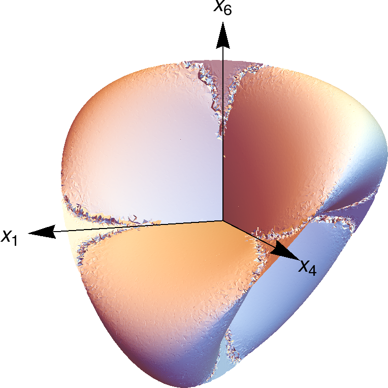
(a) Laplace coherent states of $\Pi(\mathds{C}P^{2}_{30})$.

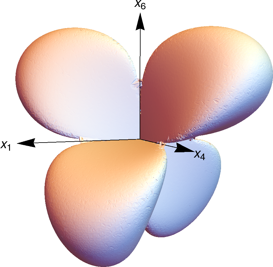
(b) Dirac coherent states of $\Pi(\mathds{C}P_{3}^{2})$.

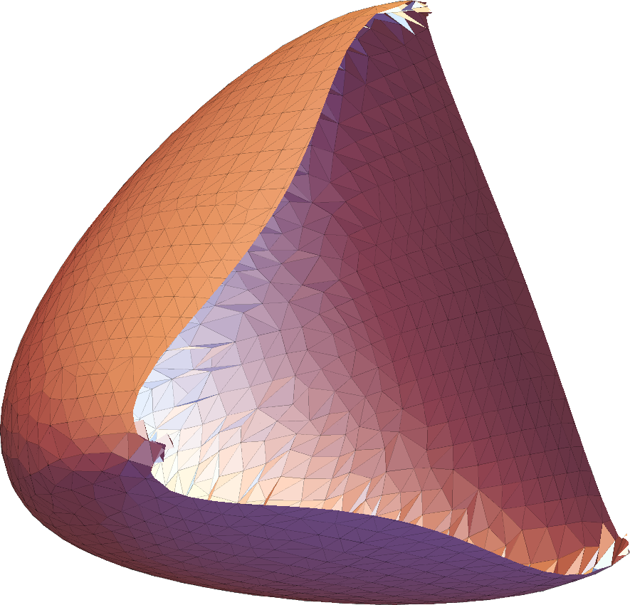
(c) A cut through one of the vaults of 8.3b to show that it is hollow.

Figure 8.3: Visualization of numerically obtained coherent states of squashed $\mathds{C}P_{N}^{2}$.

This is the first example where the Dirac coherent states do not agree with the Laplace coherent states, although some similarity can be recognized. Remarkably, the calculated points satisfy

$$E(\vec{x})<1.14\times 10^{-13}$$

which again suggests that these states are exact zero modes of the Dirac operator $\not{D}_{x}$. Indeed the general argument in section 7.3 strongly suggests that as there are two transversal dimensions, there should be two exact zero modes of $\not{D}_{x}$ at the effective location of the semi-classical 4-dimensional manifold $\mathscr{M}$. Moreover since the target space is even-dimensional, the Dirac operator anti-commutes with the 6-dimensional chirality operator, so that its zero modes must always come in pairs of two. Therefore there should be a 4-dimensional variety of exact zero modes. This is indeed seen numerically. To demonstrate this, let us consider a smooth curve $\gamma:\mathds{R}\to\mathds{R}^{3}_{135}\subset{\mathds{R}}^{6}$ through the $135$-plane, and the corresponding smooth curve of Dirac operators

$$t\mapsto\not{D}_{\gamma(t)}.$$ (8.88)

We are able to numerically generate a smooth functions $t\mapsto\lambda(t)$, where $\lambda(t)$ are eigenvalues of $\not{D}_{\gamma(t)}$, to arbitrary high resolution. Moreover we can follow these smooth functions as they pass through zero, where they cross with their chiral counterparts. This confirms the existence of zero modes on a one parameter curve $\gamma$. Let us choose the curve $\gamma$ as follows

$$\gamma(t)=\frac{1}{\sqrt{3}}\begin{pmatrix}1\\ 1\\ -1\end{pmatrix}t+\begin{pmatrix}0\\ \kappa\\ 0\end{pmatrix}e^{-(t-1/10)^{2}}$$ (8.89)

setting $\kappa=10^{-3}$. The (small) second term is added is to resolve additional degeneracies, which would occur e.g. on $\bar{\gamma}(t)=(1,1,-1)\,t$.

To get an idea of the behavior of the eigenvalues of $\not{D}_{\gamma(t)}$ we track the $12$ lowest eigenvalues on the set $\gamma([-1,1])$. They are visualized in 8.4a, and a more detailed plot of lowest two eigenvalues is given in 8.4b.

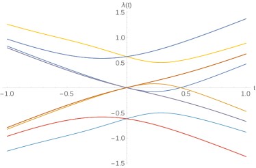
(a) A plot of the $12$ lowest eigenvalues. The highest and the third highest eigenvalues possess a multiplicity of $2$ (which can not be seen in this picture).

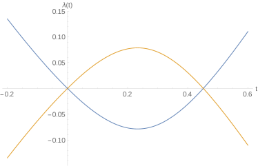
(b) A plot of the two lowest eigenvalues. They clearly exhibit two roots.

Figure 8.4: Visualization of tracked eigenvalues of $\not{D}_{\gamma(t)}$, indicated by differing colors, for $\gamma(\mathds{R})$ approximately being a straight line through the origin and the point $(1,1,-1)$.

One clearly observes the two sign changes: one at the origin and one near $\gamma(t\approx 0.45)$. Having a zero mode at $\gamma(t=0)$ is not surprising. However, the second roots near  $\gamma(t\approx 0.45)$ are not evident a priori, and could only be asserted by numerical means. This nicely confirms the discussion in section 7.3, which strongly suggests the existence of exact zero modes on a semi-classical 4-dimensional variety.

9 Conclusion

In this paper, we introduced generalized coherent states for generic quantum or fuzzy geometries defined by a set of matrices $X^{a},\ a=1,...,d$, and used them to extract the effective geometry of such a configuration. Adapting and generalizing ideas in [12, 11, 10], we propose to define quasi-coherent states as ground states of a matrix Laplacian $\boxempty_{x}$ or a matrix Dirac operator $\not{D}_{x}$ in the presence of a point brane in target space. The eigenvalues of the lowest off-diagonal modes are interpreted as displacement energy, corresponding to the energy of strings stretching between the test brane and the background brane. This string-inspired idea is independent of more traditional notions in noncommutative geometry such as spectral geometry or differential calculi, and turns out to be very powerful. These quasi-coherent states can be obtained numerically by a simple scanning procedure in target space, possibly selected by some cutoff criteria. Since they have good localization properties, the expectation values of the $X^{a}$ with these states provides a natural way to measure the location in target space, leading to an approximate location of some (possibly degenerate) variety embedded in target space. We provide analytical and numerical tests and illustrations of these ideas in various examples of fuzzy geometries.

Although similar ideas how to measure matrix geometries were put forward previously [10], we emphasize that our approach allows to address the case of a single, given matrix background, without relying on the existence of some limit $N\to\infty$. We discuss in particular ways to measure the quality of the geometric approximation, notably in terms of the hierarchy of eigenvalues of a Hessian.

In this paper, only the basic principles of an algorithm to measure such quantum geometries are presented. However, we also provide a full implementation as a Wolfram Mathematica package BProbe [40], which is open to further developments. Both approaches using the Laplacian $\boxempty_{x}$ and the Dirac operator $\not{D}_{x}$ are implemented. This nicely reproduces the expected semi-classical geometry of standard examples such as the fuzzy sphere and fuzzy tori, including the non-trivial case of squashed fuzzy $\mathds{C}P^{2}_{N}$. We hope that this should provide a useful tool to assist further studies in this field.

While our numerical procedure to collect coherent states is mainly used here to visualize the corresponding classical manifolds, they have much broader applications. The quasi-coherent states can be used to compute expectation values of various observables. For example, the observables $[X^{a},X^{b}]$ are expected to approximate a semi-classical Poisson structure, and more complicated observables such as $[X^{a},X^{b}][X_{b},X^{c}]$ are related to the effective “open string” metric as discussed in [5]. Similarly, the full differential geometry of embedded manifolds corresponding to the closed string metric could in principle be extracted [10].

One particularly interesting application of our method would be to measure the geometry of the matrix configurations obtained by numerical simulations of the IIB matrix model [15, 16, 17]. These results suggest that 3+1-dimensional cosmological backgrounds are dynamically generated. The present methods should allow a much more detailed analysis of these geometries, and we hope to be able to carry this out in the future.

Acknowledgements.

This work was supported in part by the Austrian Science Fund (FWF) grants P24713 and P28590 and by the Action MP1405 QSPACE from the European Cooperation in Science and Technology (COST). H.S. would like to thank D. Berenstein, D. O’Connor, H. Grosse, J. Karczmarek, J. Madore and A. Tsuchiya for related discussions and correspondence, and J. Zahn for related collaboration.

Appendix A Conventions for $SU(3)$

A standard orthonormal basis of $\mathfrak{su}(3)$ is given by the Gell-Mann matrices:

$$\lambda_{1}=\begin{pmatrix}0&1&0\\ 1&0&0\\ 0&0&0\end{pmatrix},\quad \lambda_{2}=\begin{pmatrix}0&-i&0\\ i&0&0\\ 0&0&0\end{pmatrix},\quad \lambda_{3}=\begin{pmatrix}1&0&0\\ 0&-1&0\\ 0&0&0\end{pmatrix},$$

$$\lambda_{4}=\begin{pmatrix}0&0&1\\ 0&0&0\\ 1&0&0\end{pmatrix},\quad \lambda_{5}=\begin{pmatrix}0&0&-i\\ 0&0&0\\ i&0&0\end{pmatrix},\quad \lambda_{6}=\begin{pmatrix}0&0&0\\ 0&0&1\\ 0&1&0\end{pmatrix},$$

$$\lambda_{7}=\begin{pmatrix}0&0&0\\ 0&0&-i\\ 0&i&0\end{pmatrix},\quad \lambda_{8}=\frac{1}{\sqrt{3}}\begin{pmatrix}1&0&0\\ 0&1&0\\ 0&0&-2\end{pmatrix}$$

We use the rescaled basis $t_{a}:=\lambda_{a}/2$, which satisfy the commutation relations

$$[t_{a},t_{b}]=i\,c_{abc}\,t_{c}$$ (A.1)

where $c_{abc}$ are the so called antisymmetric structure constants of $\mathfrak{su}(3)$ given by

$$c_{123} = 1$$ (A.2)

$$c_{147}=c_{165}=c_{246}=c_{257}=c_{345}=c_{376} = 1/2$$

$$c_{458}=c_{678} = \sqrt{3}/2,$$

while all the others vanish. They determine the structure of the Lie algebra respectively Lie group, and obey the relations

$$\sum_{a,b=1}^{8}c_{abi}c_{abj}=3\,\delta_{ij}.$$

Then the totally symmetric tensor $d_{abc}$ of $\mathfrak{su}(3)$ can be defined by the relation

$$[t_{a},t_{b}]_{+}=\frac{1}{3}\delta_{ab}+d_{abc}\,t_{c}$$ (A.3)

where $[a,b]_{+}$ is the anti-commutator. They are given by

$$d_{118}=d_{228}=d_{338}=-d_{888} = 1/\sqrt{3}$$ (A.4)

$$d_{448}=d_{558}=d_{668}=d_{778} = -1/(2\sqrt{3})$$

$$d_{146}=d_{157}=-d_{247}=d_{256}=d_{344}=d_{355}=-d_{366}=-d_{377} = 1/2.$$

The root generators (or ladder operators)

$$t_{1}^{\pm} :=t_{4}\pm it_{5},$$ (A.5)

$$t_{2}^{\pm} :=t_{6}\pm it_{7},$$

$$t_{3}^{\pm} :=t_{1}\pm it_{2}=\pm[t_{1}^{\pm},t_{2}^{\mp}].$$

together with the Cartan generators $t_{3}$ and $t_{8}$ form a Cartan-Weyl basis of $\mathfrak{su}(3)$ .

Appendix B Calculations for Coherent States of Squashed $\mathds{C}P^{2}$

B.1 Expectation values

Let the rotation $U(\boldsymbol{\varphi})$ with $\boldsymbol{\varphi}=(\varphi_{1},\varphi_{2},\varphi_{3},\varphi_{4})$ be defined as

$$U(\boldsymbol{\varphi})=e^{i\varphi_{1}T^{4}+i\varphi_{2}T^{5}+i\varphi_{3}T^{6}+i\varphi_{4}T^{7}}$$ (B.1)

with $T^{a}=\pi_{(0,N)}(t^{a})$. Additionally, let us define the rotated vector $\left|\boldsymbol{\varphi}\right\rangle$ as

$$\left|\boldsymbol{\varphi}\right\rangle:=U(\boldsymbol{\varphi})\left|\Psi_{0}\right\rangle,$$ (B.2)

where $\left|\Psi_{0}\right\rangle$ is the highest weight vector of a $(0,N)$ representation. We want to calculate the quantity

$$\vec{\bf x}(\boldsymbol{\varphi})_{a}=\left\langle\boldsymbol{\varphi}\right|X^{a}\left|\boldsymbol{\varphi}\right\rangle.$$ (B.3)

To this end consider the adjoint action of $SU(3)$ on $Mat_{M}(\mathds{C})$ given by $U^{-1}AU$ for some $A\in Mat_{M}(\mathds{C})$ and $U=\Pi_{(0,N)}(g)$ belonging to the $(0,N)$ representation. Since $Mat_{M}(\mathds{C})\doteq\bigoplus_{p=0}^{N}\mathscr{H}_{(p,p)}$ where $T^{a}\in\mathscr{H}_{(1,1)}$, the $SU(3)$ action leaves $\mathscr{H}_{(1,1)}$ invariant and we can write

$$Ad(T^{a})=U^{-1}T^{a}U=\sum_{b=1}^{8}R_{ab}T^{b}$$ (B.4)

for an orthogonal $8\times 8$ matrix $R$. Since the representations $Ad(T^{a})$ and $Ad(t^{a})$ are equivalent there exists an isomorphism $f:\mathscr{H}_{(1,1)}\to\mathfrak{su}(3)$ such that $f(Ad(T^{a}))=Ad(f(T^{a}))$. Applying $f$ to (LABEL:transformation) we get

$$Ad(t^{a})=\sum_{b=1}^{8}R_{ab}t^{b}.$$ (B.5)

Using the natural scalar product on $\mathfrak{su}(3)$ given by $(A,B):=2\,\mathrm{tr}(A\cdot B)$ chosen such that the set $\left\{t^{a},\,a=1,\dots,8\right\}$ forms an orthonormal basis we can explicitly calculate the matrix coefficients of $R$ via

$$R_{ab}=(t^{a},\,Ad(t^{b}))=2\,\mathrm{tr}(t^{a}U^{-1}t^{b}U)$$ (B.6)

which for $U=U(\boldsymbol{\varphi})$ can be carried out by computer algebra systems. Expression (B.3) can now be written as

$$\vec{\bf x}(\boldsymbol{\varphi})_{a}=\sum_{b=1}^{8}R_{ab}\left\langle\Psi_{0}\right|X^{b}\left|\Psi_{0}\right\rangle=c_{N}\sum_{b=1}^{8}R_{ab}\left\langle\Psi_{0}\right|T^{b}\left|\Psi_{0}\right\rangle$$

and since $\left\langle\Psi_{0}\right|T^{8}\left|\Psi_{0}\right\rangle=\frac{N}{\sqrt{3}}$ is the only non-zero component we get

$$\vec{\bf x}(\boldsymbol{\varphi})_{a}=c_{N}R_{a8}\frac{N}{\sqrt{3}}$$

and after plugging in the coefficients $R_{a8}$ we recover (LABEL:location_scp2):

$$\vec{\bf x}(\boldsymbol{\varphi}) =c_{N}\frac{N}{2}\frac{1}{|\boldsymbol{\varphi}|}\begin{pmatrix}\frac{(\varphi_{1}\varphi_{3}+\varphi_{2}\varphi_{4})}{|\boldsymbol{\varphi}|}(\cos|\boldsymbol{\varphi}|-1)\\ 2\frac{(\varphi_{1}\varphi_{4}-\varphi_{2}\varphi_{3})}{|\boldsymbol{\varphi}|}\sin^{2}\frac{|\boldsymbol{\varphi}|}{2}\\ \varphi_{2}\,\sin|\boldsymbol{\varphi}|\\ -\varphi_{1}\,\sin|\boldsymbol{\varphi}|\\ \varphi_{4}\,\sin|\boldsymbol{\varphi}|\\ -\varphi_{3}\,\sin|\boldsymbol{\varphi}|\end{pmatrix}.$$ (B.7)

B.2 Dispersion

Next we want to evaluate the dispersion (4.16) which reads

$$\updelta(\boldsymbol{\varphi})=1-\sum_{i=3,8}\left\langle\boldsymbol{\varphi}\right|(X^{i})^{2}\left|\boldsymbol{\varphi}\right\rangle-|\vec{x}(\boldsymbol{\varphi})|^{2}.$$ (B.8)

Having calculated the third term already we are left with the second term $\sum_{i=3,8}\left\langle\boldsymbol{\varphi}\right|(X^{i})^{2}\left|\boldsymbol{\varphi}\right\rangle$ which can be written as

$$\sum_{i=3,8}\left\langle\boldsymbol{\varphi}\right|(X^{i})^{2}\left|\boldsymbol{\varphi}\right\rangle=\sum_{i=3.8}\sum_{a,b=1}^{8}R_{ia}R_{ib}\left\langle\Psi_{0}\right|X^{a}X^{b}\left|\Psi_{0}\right\rangle.$$ (B.9)

The expression $M_{ab}:=\left\langle\Psi_{0}\right|X^{a}X^{b}\left|\Psi_{0}\right\rangle=c_{N}^{2}\left\langle\Psi_{0}\right|T^{a}T^{b}\left|\Psi_{0}\right\rangle$ can be calculated explicitly and yields

$$M=c_{N}^{2}\frac{N}{4}\begin{pmatrix}0&0&0&0&0&0&0&0\\ 0&0&0&0&0&0&0&0\\ 0&0&0&0&0&0&0&0\\ 0&0&0&1&i&0&0&0\\ 0&0&0&-i&1&0&0&0\\ 0&0&0&0&0&1&i&0\\ 0&0&0&0&0&-i&1&0\\ 0&0&0&0&0&0&0&\frac{4}{3}N\end{pmatrix}.$$ (B.10)

With this we can compute (B.9) and get a long expression for the second term

$$\sum_{i=3,8}\left\langle\boldsymbol{\varphi}\right|(X^{i})^{2}\left|\boldsymbol{\varphi}\right\rangle =c_{N}^{2}\frac{N}{48}\frac{1}{|\boldsymbol{\varphi}|^{4}}e^{-2i|\boldsymbol{\varphi}|}\times$$

$$\times \left(12e^{i|\boldsymbol{\varphi}|}(N-1)(\varphi_{1}^{2}+\varphi_{2}^{2})(\varphi_{3}^{2}+\varphi_{4}^{2})+12e^{3i|\boldsymbol{\varphi}|}(N-1)(\varphi_{1}^{2}+\varphi_{2}^{2})(\varphi_{3}^{2}+\varphi_{4}^{2})\right.$$

$$+ 3(N-1)\left(\varphi_{1}^{4}+\varphi_{2}^{4}+\varphi_{2}^{2}(\varphi_{3}^{2}+\varphi_{4}^{2})+(\varphi_{3}^{2}+\varphi_{4}^{2})^{2}+\varphi_{1}^{2}(2\varphi_{2}^{2}+\varphi_{3}^{2}+\varphi_{4}^{2})\right)$$

$$+ 3e^{4i|\boldsymbol{\varphi}|}(N-1)\left(\varphi_{1}^{4}+\varphi_{2}^{4}+\varphi_{2}^{2}(\varphi_{3}^{2}+\varphi_{4}^{2})+(\varphi_{3}^{2}+\varphi_{4}^{2})^{2}+\varphi_{\text{1}}^{2}(2\varphi_{2}^{2}+\varphi_{3}^{2}+\varphi_{4}^{2})\right)$$

$$+ 2e^{2i|\boldsymbol{\varphi}|}\left((3+5n)\varphi_{1}^{4}+(3+5n)\varphi_{2}^{4}+(15+N)\varphi_{2}^{2}(\varphi_{3}^{2}+\varphi_{4}^{2})+(3+5m)(\varphi_{3}^{2}+\varphi_{4}^{2})^{2}\right.$$

$$\left.\left.+\varphi_{1}^{2}\left(2(3+m)\varphi_{2}^{2}+(15+m)(\varphi_{3}^{2}+\varphi_{4}^{2})\right)\right)\vphantom{12e^{i|\boldsymbol{\varphi}|}}\right).$$ (B.11)

Plugging (B.7) and (B.11) into (LABEL:disp_squashed-calc) and simplifying thankfully yields a more compact relation for the dispersion

$$\updelta(\boldsymbol{\varphi})= \frac{3}{8\,(3+N)}\frac{1}{|\boldsymbol{\varphi}|^{4}}\left\{4(\varphi_{1}^{2}+\varphi_{2}^{2})(\varphi_{3}^{2}+\varphi_{4}^{2})\cos|\boldsymbol{\varphi}|\right.$$

$$+ \left.\left(\varphi_{1}^{4}+\varphi_{2}^{4}+\varphi_{1}^{2}(2\,\varphi_{2}^{2}+\varphi_{3}^{2}+\varphi_{4}^{2})+\varphi_{2}^{2}(\varphi_{3}^{2}+\varphi_{4}^{2})+(\varphi_{3}^{2}+\varphi_{4}^{2})^{2}\right)\cos 2|\boldsymbol{\varphi}|\right.$$

$$+ \left.\left(7\,(\varphi_{1}^{4}+\varphi_{2}^{4})+7\,(\varphi_{3}^{2}+\varphi_{4}^{2})^{2}+11\,\varphi_{2}^{2}(\varphi_{3}^{2}+\varphi_{4}^{2})\right)\right\}$$ (B.12)

which concludes the calculation.

References

- [1] N. Ishibashi, H. Kawai, Y. Kitazawa, and A. Tsuchiya, A Large N reduced model as superstring, Nucl. Phys. B498, 467 (1997), hep-th/9612115.
- [2] T. Banks, W. Fischler, S. H. Shenker, and L. Susskind, M theory as a matrix model: A Conjecture, Phys. Rev. D55, 5112 (1997), hep-th/9610043.
- [3] J. R. Hoppe, Quantum Theory of a Massless Relativistic Surface and a Two-Dimensional Bound State Problem., PhD thesis, MASSACHUSETTS INSTITUTE OF TECHNOLOGY., 1982.
- [4] J. Madore, The Fuzzy sphere, Class. Quant. Grav. 9, 69 (1992).
- [5] H. Steinacker, Emergent Geometry and Gravity from Matrix Models: an Introduction, Class. Quant. Grav. 27, 133001 (2010), 1003.4134.
- [6] H. Steinacker, Emergent Gravity and Noncommutative Branes from Yang-Mills Matrix Models, Nucl. Phys. B810, 1 (2009), 0806.2032.
- [7] A. M. Perelomov, Generalized coherent states and their applications (Springer-Verlag, 1986).
- [8] H. Grosse and P. Presnajder, The Construction on noncommutative manifolds using coherent states, Lett. Math. Phys. 28, 239 (1993).
- [9] A. P. Balachandran, S. Kurkcuoglu, and S. Vaidya, Lectures on fuzzy and fuzzy SUSY physics, (2005), hep-th/0511114.
- [10] G. Ishiki, Matrix Geometry and Coherent States, Phys. Rev. D92, 046009 (2015), 1503.01230.
- [11] D. Berenstein and E. Dzienkowski, Matrix embeddings on flat and the geometry of membranes, Phys. Rev. D86, 086001 (2012), 1204.2788.
- [12] A. Chatzistavrakidis, H. Steinacker, and G. Zoupanos, Intersecting branes and a standard model realization in matrix models, JHEP 09, 115 (2011), 1107.0265.
- [13] H. C. Steinacker, Spinning squashed extra dimensions and chiral gauge theory from N=4 SYM, Nucl. Phys. B896, 212 (2015), 1411.3139.
- [14] H. C. Steinacker, Chiral low-energy physics from squashed branes in deformed SYM, JHEP 10, 119 (2015), 1504.05703.
- [15] S.-W. Kim, J. Nishimura, and A. Tsuchiya, Late time behaviors of the expanding universe in the IIB matrix model, JHEP 10, 147 (2012), 1208.0711.
- [16] Y. Ito, J. Nishimura, and A. Tsuchiya, Power-law expansion of the Universe from the bosonic Lorentzian type IIB matrix model, JHEP 11, 070 (2015), 1506.04795.
- [17] S.-W. Kim, J. Nishimura, and A. Tsuchiya, Expanding (3+1)-dimensional universe from a Lorentzian matrix model for superstring theory in (9+1)-dimensions, Phys. Rev. Lett. 108, 011601 (2012), 1108.1540.
- [18] R. Dijkgraaf, E. P. Verlinde, and H. L. Verlinde, Matrix string theory, Nucl. Phys. B500, 43 (1997), hep-th/9703030.
- [19] S. Waldmann, Poisson-Geometrie (Springer, 2007).
- [20] G. Alexanian, A. P. Balachandran, G. Immirzi, and B. Ydri, Fuzzy CP**2, J. Geom. Phys. 42, 28 (2002), hep-th/0103023.
- [21] H. Grosse and H. Steinacker, Finite gauge theory on fuzzy CP**2, Nucl. Phys. B707, 145 (2005), hep-th/0407089.
- [22] A. P. Balachandran, B. P. Dolan, J.-H. Lee, X. Martin, and D. O’Connor, Fuzzy complex projective spaces and their star products, J. Geom. Phys. 43, 184 (2002), hep-th/0107099.
- [23] J. Pawelczyk and H. Steinacker, A Quantum algebraic description of D branes on group manifolds, Nucl. Phys. B638, 433 (2002), hep-th/0203110.
- [24] H. C. Steinacker and J. Zahn, Self-intersecting fuzzy extra dimensions from squashed coadjoint orbits in SYM and matrix models, JHEP 02, 027 (2015), 1409.1440.
- [25] J. Castelino, S. Lee, and W. Taylor, Longitudinal five-branes as four spheres in matrix theory, Nucl. Phys. B526, 334 (1998), hep-th/9712105.
- [26] J. Medina and D. O’Connor, Scalar field theory on fuzzy S**4, JHEP 11, 051 (2003), hep-th/0212170.
- [27] H. C. Steinacker, One-loop stabilization of the fuzzy four-sphere via softly broken SUSY, JHEP 12, 115 (2015), 1510.05779.
- [28] H. Weyl, Gruppentheorie und Quantenmechanik (Hirzel, Leipzig, 1928).
- [29] J. Radcliffe, Some properties of coherent spin states, Journal of Physics A: General Physics 4, 313 (1971).
- [30] A. O. Barut and L. Girardello, New ’coherent’ states associated with noncompact groups, Commun. Math. Phys. 21, 41 (1971).
- [31] H. Grosse and P. Prešnajder, The construction of noncommutative manifolds using coherent states, Letters in Mathematical Physics 28, 239 (1993).
- [32] J.-P. Gazeau, Coherent states in quantum physics (Wiley, 2009).
- [33] S. Andronache and H. C. Steinacker, The squashed fuzzy sphere, fuzzy strings and the Landau problem, J. Phys. A48, 295401 (2015), 1503.03625.
- [34] S. Ramgoolam, On spherical harmonics for fuzzy spheres in diverse dimensions, Nucl. Phys. B610, 461 (2001), hep-th/0105006.
- [35] P. Zezula, G. Amato, V. Dohnal, and M. Batko, Similarity Search - The Metric Space Approach, Advances in Database Systems Vol. 32 (Kluwer, 2006).
- [36] D. A. Watt and W. Findlay, Programming language design concepts. (Wiley, 2004).
- [37] J. L. Karczmarek and K. H.-C. Yeh, Noncommutative spaces and matrix embeddings on flat , JHEP 11, 146 (2015), 1506.07188.
- [38] M. H. de Badyn, J. L. Karczmarek, P. Sabella-Garnier, and K. H.-C. Yeh, Emergent geometry of membranes, JHEP 11, 089 (2015), 1506.02035.
- [39] H. Steinacker and J. Zahn, An Index for Intersecting Branes in Matrix Models, SIGMA 9, 067 (2013), 1309.0650.
- [40] L. Schneiderbauer, BProbe: a Wolfram Mathematica package, 2016, doi:10.5281/zenodo.45045.