Efficient Robust Mean Value Calculation
of 1D Features

Abstract

A robust mean value is often a good alternative to the standard mean value when dealing with data containing many outliers. An efficient method for samples of one-dimensional features and the truncated quadratic error norm is presented and compared to the method of channel averaging (soft histograms).

1 Introduction

In a lot of applications in image processing we are faced with data containing lots of outliers. One example is denoising and edge-preserving smoothing of low-level image features, but the outlier problem also occurs in high-level operations like object recognition and stereo vision. A wide range of robust techniques for different applications have been presented, where RANSAC [5] and the Hough transform [7] are two classical examples.

In this paper, we focus on the particular problem of calculating a mean value which is robust against outliers. An efficient method for the special case of one-dimensional features is presented and compared to the channel averaging [3] approach.

2 Problem Formulation

Given a sample set $\mathbf{X}=[\mathbf{x}^{(1)}\ldots\mathbf{x}^{(n)}]$, we seek to minimize an error function given by

$$\mathcal{E}(\mathbf{x})=\sum_{k=1}^{n}\rho(\|\mathbf{x}^{(k)}-\mathbf{x}\|)$$ (1)

If we let $\rho$ be a quadratic function, the minimizing $\mathbf{x}$ is the standard mean value. To achieve the desired robustness against outliers, $\rho$ should be a function that saturates for large argument values. Such functions are called robust error norms. Some popular choices are the truncated quadratic and Tukey’s biweight shown in figure 1. A simple 1D data set together with its error function is shown in figure 2. The $\mathbf{x}$ which minimizes (1) belongs to a general class of estimators called M-estimators [8], and will in this text be referred to as the robust mean value.

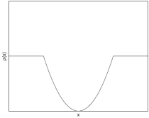
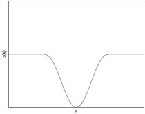
Figure 1: Error norms: Truncated quadratic (left), Tukey’s biweight (right)

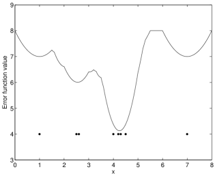
Figure 2: A simple 1D data set together with the error function generated using the truncated quadratic error norm with cutoff distance 1

3 Previous Work

Finding the robust mean is a non-convex optimization problem, and a unique global minimum is not guaranteed. The problem is related to clustering, and the well-known mean shift iteration has been shown to converge to a local minimum of a robust error function [1].

Another approach is to use the channel representation (soft histograms) [2, 3, 4, 6]. Each sample $\mathbf{x}$ can be encoded into a channel vector $\mathbf{c}$ by the nonlinear transformation

$$\mathbf{c}=[K(\|\mathbf{x}-\xi_{1}\|),\ldots,K(\|\mathbf{x}-\xi_{m}\|)]$$ (2)

where $K$ is a localized kernel function and $\xi_{k}$ the channel centers, typically located uniformly and such that the kernels overlap (fig 3). By averaging the channel representations of the samples, we get something which resembles a histogram, but with overlapping and “smooth” bins. Depending on the choice of kernel, the representation can be decoded to obtain an approximate robust mean. The distance between neighboring channels corresponds to the scale of the robust error norm.

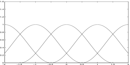
Figure 3: Example of channel kernel functions located at the integers

4 Efficient 1D Method

This section will cover the case where the $\mathbf{x}$’s are one-dimensional, e.g. intensities in an image, and the truncated quadratic error norm is used. In this case, there is a very efficient method, which we have not discovered in the literature. For clarity, we describe the case where all samples have equal weight, but the extension to weighted samples is straightforward.

First, some notation. We assume that our data is sorted in ascending order and numbered from $1\ldots n$. Since the $\mathbf{x}$’s are one dimensional, we drop the vector notation and write simply $x_{k}$. The error norm is truncated at $c$, and can be written as

$$\rho(x)=\min\{x^{2},c^{2}\}$$ (3)

The method works as follows: We keep track of indices $a,b$ and and a window $w=[a,b]$ of samples $[x_{a},\ldots,x_{b}]$. The window $[a,b]$ is said to be

• feasible if $|x_{b}-x_{a}|<2c$

• maximal if the samples are contained in a continuous window of length $2c$, i.e. if $[a,b]$ is feasible and $[a-1,b+1]$ is infeasible.

Now define for a window $w=[a,b]$

$$\mu_{w} = \frac{1}{b-a+1}\sum_{k=a}^{b}x_{k}$$ (4)

$$n_{o} = (a-1)+(n-b)\quad$$ (5)

$$q_{w} = \sum_{k=a}^{b}(\mu_{w}-x_{k})^{2}$$ (6)

$$\hat{\mathcal{E}}_{w} = q_{w}+n_{o}c^{2}$$ (7)

Note that $n_{o}$ is the number of samples outside the window. Consider the global minimum $x_{0}$ of the error function and the window $w$ of samples $x_{k}$ that fall within the quadratic part of the error function centered around $x_{0}$, i.e. the samples $x_{k}$ such that $|x_{k}-x_{0}|\leq c$. Either this window is located close to the boundary ($a=1$ or $b=n$) or constitutes a maximal window. In both cases, $x_{0}=\mu_{w}$, and $\hat{\mathcal{E}}_{w}=\mathcal{E}(\mu_{w})$. This is not necessarily true for an arbitrary window, e.g. if $\mu_{w}$ is located close to the window boundary. However, for an arbitrary window $w$, we have

$$\hat{\mathcal{E}}_{w} = \sum_{k=a}^{b}(\mu_{w}-x_{k})^{2}+n_{o}c^{2}\geq$$ (8)

$$\geq \sum_{k=1}^{n}\min\{(\mu_{w}-x_{k})^{2},c^{2}\}$$ (9)

$$= \sum_{k=1}^{n}\rho(\mu_{w}-x_{k})=\mathcal{E}(\mu_{w})$$ (10)

The strategy is now to enumerate all maximal and boundary windows, evaluate $\hat{\mathcal{E}}_{w}$ for each and take the minimum, which is guaranteed to be the global minimum of $\mathcal{E}$. Note that it does not matter if some non-maximal windows are included, since we always have $\hat{\mathcal{E}}_{w}\geq\mathcal{E}(\mu_{w})$.

The following iteration does the job: Assume that we have a feasible window $[a,b]$, not necessarily maximal. If $[a,b+1]$ is feasible, take this as the new window. Otherwise, $[a,b]$ was the largest maximal window starting at $a$, and we should go on looking for maximal windows starting at $a+1$. Take $[a+1,b]$ as the first candidate, then keep increasing $b$ until the window becomes infeasible, etc. If proper initialization and termination of the loop is provided, this iteration will generate all maximal and boundary windows.

The last point to make is that we do not need to recompute $q_{w}$ from scratch as the window size is changed. Similar to the treatment of mean values and variances in statistics, we get by expanding the quadratic expression

$$q_{w} = \sum_{k=a}^{b}(\mu_{w}-x_{k})^{2}=$$ (11)

$$= \sum_{k=a}^{b}x_{k}^{2}-(b-a+1)\mu_{w}^{2}=$$

$$= S_{2}-(b-a+1)^{-1}S_{1}^{2}$$

where we have defined

$$S_{1} = \sum_{k=a}^{b}x_{k}=(b-a+1)\mu_{w}$$ (12)

$$S_{2} = \sum_{k=a}^{b}x_{k}^{2}$$ (13)

$S_{1}$ and $S_{2}$ can easily be updated in constant time as the window size is increased or decreased, giving the whole algorithm complexity $O(n)$. The algorithm is summarized as follows:

Algorithm 1 Fast 1D robust mean calculation

  Initialize $a\leftarrow 1$, $b\leftarrow 1$, $S_{1}\leftarrow x_{1}$, $S_{2}\leftarrow x_{1}^{2}$

  while $a\leq n$ do

     if $a\leq b$ then

        Calculate candidate $\hat{\mathcal{E}}_{w}$ and $\mu_{w}$:

        $\mu_{w}\leftarrow(b-a+1)^{-1}S_{1}$

        $\hat{\mathcal{E}}_{w}\leftarrow S_{2}-\mu_{w}S_{1}+n_{o}c^{2}$

        If $\hat{\mathcal{E}}_{w}$ is the smallest so far, store $\hat{\mathcal{E}}_{w}$, $\mu_{w}$.

     end if

     if $b<n$ and $|x_{b+1}-x_{a}|<2c$ then

        $b\leftarrow b+1$

        $S_{1}\leftarrow S_{1}+x_{b}$

        $S_{2}\leftarrow S_{2}+x_{b}^{2}$

     else

        $S_{1}\leftarrow S_{1}-x_{a}$

        $S_{2}\leftarrow S_{2}-x_{a}^{2}$

        $a\leftarrow a+1$

     end if

  end while

  The $\mu_{w}$ corresponding to the smallest $\hat{\mathcal{E}}_{w}$ is now the robust mean.

Note that it is straightforward to introduce a weight $w$ for each sample, such that a weighted mean value is produced. We should then let $n_{0}$ be the total weight of the samples outside the window, $\mu_{w}$ the weighted mean value of the window $w$, $S_{1}$ and $S_{2}$ weighted sums etc.

5 Properties of the Robust
Mean Value

In this section, some properties of the robust mean values generated by the truncated quadratic method and the channel averaging will be examined. In figure 4, we show the robust mean of a sample set consisting of some values (inliers) with mean value $3.0$ and an outlier at varying positions. As the outlier moves sufficiently far away from the inliers, it is completely rejected, and when it is close to $3.0$, it is treated as an inlier. As expected, the truncated quadratic method makes a hard decision about whether the outlier should be included or not, whereas the channel averaging implicitly assumes a smoother error norm.

Another effect is that the channel averaging overcompensates for the outlier at some positions (around $x=6.0$ in the plot). Also, the exact behavior of the method can vary at different absolute positions due to the grid effect illustrated in figure 5. We calculated the robust mean of two samples $x_{1},x_{2}$, symmetrically placed around some point $x_{0}$ with $|x_{1}-x_{0}|=|x_{2}-x_{1}|=d$. The channels were placed with unit distance, and the displacement of the estimated mean $m$ compared to the desired value $x_{0}$ is shown for varying $x_{0}$’s in the range between two neighboring channel centers. The figure shows that the method makes some (small) systematic errors depending on the position relative to the channel grid. No such grid effect occurs using the method from section 4.

When the robust mean algorithm is applied on sliding spatial windows of an image, we get an edge-preserving image smoothing method. In figure 6, we show the 256x256 Lenna image smoothed with the truncated quadratic method using a spatial window of 5 x 5 and $c=0.1$ in the intensity domain, where intensities are in the range $[0,1]$. The pixels are weighted with a Gaussian function.

Figure 4: The influence of an outlier on the mean value

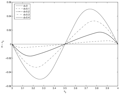
Figure 5: The grid effect

6 Discussion

We have shown an efficient way to calculate the robust mean value for the special case of one-dimensional features and the truncated quadratic error. The advantage of this method is that it is simple, exact and global. The disadvantage is of course its limitation to one-dimensional feature spaces.

One example of data for which the method could be applied is image features like intensity or orientation. If the number of samples is high, e.g. in robust smoothing of a high resolution image volume, the method might be suitable. If a convolution-like operation is to be performed, the overhead of sorting the samples could be reduced significantly, since the data is already partially sorted when moving to a new spatial window, leading to an efficient edge-preserving smoothing algorithm.

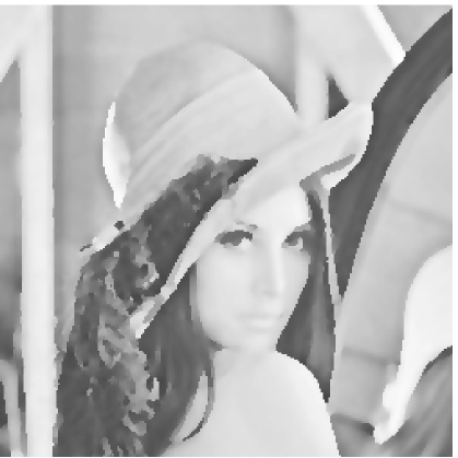
Figure 6: Lenna, robustly smoothed with the truncated quadratic method

References

- [1] Y Cheng. Mean shift, mode seeking and clustering. IEEE Transactions on Pattern Analysis and Machine Intelligence, 17(8):790–799, 1995.
- [2] M. Felsberg. Auto-associative feature processing. In Early Cognitive Vision Workshop, Isle of Skye, Scotland, 2004.
- [3] M. Felsberg and G. Granlund. Anisotropic channel filtering. In Proc. 13th Scandinavian Conference on Image Analysis, LNCS 2749, pages 755–762, Gothenburg, Sweden, 2003.
- [4] M. Felsberg and G.H. Granlund. POI detection using channel clustering and the 2D energy tensor. In 26. DAGM Symposium Mustererkennung, Tübingen, 2004.
- [5] R. Hartley and A. Zisserman. Multiple View Geometry in Computer Vision. Cambridge University Press, 2001.
- [6] H. Scharr, M. Felsberg, and P.-E. Forssén. Noise adaptive channel smoothing of low-dose images. In CVPR Workshop: Computer Vision for the Nano-Scale, 2003.
- [7] M. Sonka, V. Hlavac, and R. Boyle. Image Processing, Analysis, and Machine Vision. Brooks / Cole, 1999.
- [8] G. Winkler and V. Liebscher. Smoothers for discontinuous signals. Nonparametric Statistics, 14:203–222, 2002.