Adaptive scaling for soft-thresholding estimator

Abstract

Soft-thresholding is a sparse modeling method that is typically applied to wavelet denoising in statistical signal processing and analysis. It has a single parameter that controls a threshold level on wavelet coefficients and, simultaneously, amount of shrinkage for coefficients of un-removed components. This parametrization is possible to cause excess shrinkage, thus, estimation bias at a sparse representation; i.e. there is a dilemma between sparsity and prediction accuracy. To relax this problem, we considered to introduce positive scaling on soft-thresholding estimator, by which threshold level and amount of shrinkage are independently controlled. Especially, in this paper, we proposed component-wise and data-dependent scaling in a setting of non-parametric orthogonal regression problem including discrete wavelet transform. We call our scaling method adaptive scaling. We here employed soft-thresholding method based on LARS(least angle regression), by which the model selection problem reduces to the determination of the number of un-removed components. We derived a risk under LARS-based soft-thresholding with the proposed adaptive scaling and established a model selection criterion as an unbiased estimate of the risk. We also analyzed some properties of the risk curve and found that the model selection criterion is possible to select a model with low risk and high sparsity compared to a naive soft-thresholding method. This theoretical speculation was verified by a simple numerical experiment and an application to wavelet denoising.

1 Introduction

Orthogonal transform such as discrete wavelet transform is an important tool in statistical signal processing and analysis. Especially, wavelet denoising is a popular application of discrete wavelet transform. In wavelet denoising, noisy signal is transformed into wavelet domain in which wavelet coefficients are obtained. By applying a thresholding method, noise-related parts of coefficients are removed in a sense; e.g. some of coefficients are set to zero. The inverse wavelet transform of the modified coefficients yields a denoised signal. The most popular and simple methods of thresholding is hard and soft-thresholding in [3, 4]. Both thresholding methods have a parameter. In hard-thresholding method, the parameter works purely as a threshold level; i.e. coefficients less than the parameter value are removed and un-removed coefficients are harmless. On the other hand, in soft-thresholding, the parameter works as a threshold level as in hard-thresholding and simultaneously as an amount of shrinkage for un-removed components. Coefficients less than the parameter value are removed and un-removed coefficients are shrunk toward zero by the parameter. For a better denoising performance, we need to determine an optimal value of the parameter. For example, in hard-thresholding, if the parameter value is too large then most of coefficients are removed even when those are significant. This results in an excess smoothing that yields a large bias between estimated output and target function output. On the other hand, if the parameter value is too small then most of coefficients are un-removed even when those are not significant. This results in a large variance of output estimate and, thus useless for denoising. A problem of choice of an optimal parameter value is often referred as a model selection problem. There are several model selection methods under thresholding. [3] has proposed universal hard and soft-thresholding in which a theoretically significant constant value is employed as a parameter value. Also, [3] has derived a criterion for determining an optimal parameter value of soft-thresholding by applying Stein’s lemma[15]. The soft-thresholding method with this criterion is called as SURE (Stein’s Unbiased Risk Estimator) shrink in [3]. Unfortunately, there is no such a theoretically supported criterion for hard-thresholding while modified cross validation approaches have been proposed [13, 10].

We focus on a soft-thresholding method in this paper. As previously mentioned, soft-thresholding is a combination of hard-thresholding and shrinkage in which both of threshold level and amount of shrinkage are simultaneously controlled by a single parameter. The parameter is a threshold level for removing un-necessary components and is also an amount of shift by which estimators of coefficients of un-removed components are shrunk toward to zero. If the parameter value is large then threshold level is large. Therefore, the number of un-removed components is small. However, at the same time, the amount of shrinkage is automatically large. This can be an excess shrinkage amount which may yields a large bias of output estimate in representing a target function. This may cause a high prediction error at a relatively small model even when it can represent a target function; i.e. even when it can obtain a sparse representation. Therefore, the number of un-removed components in soft-thresholding tends to be large if we choose the parameter value based on a substitution of prediction error such as SURE and cross-validation error. This is an inevitable problem of soft-thresholding, which is brought about by an introduction of a single parameter for controlling both of threshold level and amount of shrinkage simultaneously. Note that, in the implementation of thresholding methods for wavelet denoising in [3], thresholding is recommended to apply only to detail coefficients. This heuristics may be actually valid to avoid the problem mentioned here.

On the other hand, in machine learning and statistics, there are several model selection methods by using regularization, in which coefficient estimators are obtained by minimizing a regularized cost that consists of error term plus regularization term. A regularization method has a parameter that is multiplied by regularizer in the regularization term and determines a balance between error and regularization. LASSO (Least Absolute Shrinkage and Selection Operator) is a very popular regularization method for variable selection[16]. It employs sum of absolute values of coefficients as a regularizer; i.e. $\ell_{1}$ norm of a coefficient vector. LASSO is known to be useful for obtaining a sparse representation of a target function; i.e. the number of components for representing a target function is very small. In LASSO, extra components are automatically removed by setting their coefficients to zero. This property is clearly understood when it applied to orthogonal regression problems. In this case, LASSO reduces to a soft-thresholding method in which a parameter of soft-thresholding is a regularization parameter divided by 2. Hence, a sparseness obtained by LASSO comes from a sof-thresholding property. And, thus, LASSO encounters the above mentioned problem of soft-thresholding. This dilemma between sparsity and prediction of LASSO has already been discussed in [6] and [18]. [6] has proposed SCAD (Smoothly Clipped Absolute Deviation) penalty which is a nonlinear modification of $\ell_{1}$ penalty. [18] has proposed adaptive LASSO that employs weighted $\ell_{1}$ penalties. An $\ell_{1}$ penalty term is modified by different ways (functions) in SCAD and adaptive LASSO while shrinkage is suppressed for large values of estimators in both methods. This may reduce an excess shrinkage at a relatively small model. Especially, in case of orthogonal regression, weights of adaptive LASSO are effective for directly and adaptively reducing a shrinkage amount that is represented as a shift in soft-thresholding. In these methods, cross validation is used as a model selection method for choosing parameter values such as a regularization parameter. Unfortunately, usual cross validation can not be used in orthogonal regression unless it is heuristically modified as in [13, 10].

In this paper, we introduce a scaling of soft-thresholding estimators; i.e. a soft-thresholding estimator is multiplied by a scaling parameter. Unlike adaptive LASSO, introduction of scaling is intended to control threshold level and amount of shrinkage independently. It is thus a direct solution for a problem of parametrization of soft-thresholding. If the scaling parameter value is less than one then it works as shrinkage of soft-thresholding estimator. For an orthogonal regression problem, this is equivalent to elastic net[20] in machine learning. However, the scaling parameter can be larger than one by which the above mentioned excess shrinkage in soft-thresholding is expected to be relaxed; i.e. scaling expands a shrinkage estimator obtained by soft-thresholding. Especially in this paper, we propose a component-wise and data-dependent scaling method; i.e. scaling parameter value can be different for each coefficient and is calculated from data. We refer the proposed scaling as adaptive scaling. In this paper, we derive a risk under adaptive scaling and construct a model selection criterion as an unbiased risk estimate. Therefore, our work establishes a denoising method in which a drawback of a naive soft-thresholding is improved by the introduction of adaptive scaling and an optimal model is automatically selected according to a derived criterion under the adaptive scaling.

In Section 2, we state a setting of orthogonal non-parametric regression that includes a problem of wavelet denoising. In this section, we also give a naive soft-thresholding method and several related methods. In this paper, especially, we employ a soft-thresholding method based on LARS (least angle regression)[5] in these methods. In LARS-based soft-thresholding, a model selection problem reduces to the determination of the number of un-removed components. In Section 3, we define an adaptive scaling and derive a risk under LARS-based soft-thresholding with the adaptive scaling. We then give a model selection criterion as an unbiased estimate of the risk. We here also consider the properties of risk curve and reveals the model selection property. The proofs of theorems in this section are included in Appendix with some lemmas. In Section 4, the proposed adaptive scaling method is examined for toy artificial problems including applications to wavelet denoising. Section 5 is devoted to conclusions and future works.

2 Non-parametric orthogonal regression

2.1 Setting and assumption of orthogonal non-parametric regression

Let ${\boldsymbol{x}}=(x_{1},\ldots,x_{m})$ and $y$ be input variables and an output variable, for which we have $n$ i.i.d. samples : $\{({\boldsymbol{x}}_{i},y_{i}):i=1,\ldots,n\}$, where ${\boldsymbol{x}}_{i}=(x_{i,1},\ldots,x_{i,m})$. We assume that $y_{i}=h({\boldsymbol{x}}_{i})+e_{i}$, $i=1,\ldots,n$, where $e_{1},\ldots,e_{n}$ are i.i.d additive noise sequence according to $N(0,\sigma^{2})$; i.e. normal distribution with mean $0$ and variance $\sigma^{2}$. $h$ is a target function. We assume that ${\boldsymbol{x}}_{1},\ldots,{\boldsymbol{x}}_{n}$ are fixed below. We define ${\boldsymbol{y}}=(y_{1},\ldots,y_{n})^{\prime}$, ${\boldsymbol{h}}=(h({\boldsymbol{x}}_{1}),\ldots,h({\boldsymbol{x}}_{n}))^{\prime}$ and ${\boldsymbol{e}}=(e_{1},\ldots,e_{n})^{\prime}$, where ^′ denotes a matrix transpose. We then have ${\boldsymbol{y}}={\boldsymbol{h}}+{\boldsymbol{e}}$ and $\mathbb{E}[{\boldsymbol{y}}]={\boldsymbol{h}}$, where $\mathbb{E}$ denotes the expectation with respect to the joint probability distribution of ${\boldsymbol{y}}$.

Let $g_{1},g_{2},\ldots$ be a series of functions on $\mathbb{R}^{m}$. We consider to estimate a target function by a linear combination of $n$ functions in this series :

$$f_{{\boldsymbol{b}}}({\boldsymbol{x}})=\sum_{j=1}^{n}b_{j}g_{j}({\boldsymbol{x}}),~{}{\boldsymbol{x}}\in\mathbb{R}^{m},$$ (1)

where ${\boldsymbol{b}}=(b_{1},\ldots,b_{n})^{\prime}$ is a coefficient vector. This is a non-parametric regression problem. We call $g_{j}$ a component or basis function. We assume that there exists $n^{*}$ and ${\boldsymbol{\beta}}=(\beta_{1},\ldots,\beta_{n})^{\prime}$ such that $h({\boldsymbol{x}})=\sum_{j=1}^{n}\beta_{j}g_{j}({\boldsymbol{x}})$ for any ${\boldsymbol{x}}\in\mathbb{R}^{m}$ when $n\geq n^{*}$. $\beta_{j}$ can be zero for some $j$. We define $K^{*}=\{j:1\leq j\leq n,~{}\beta_{j}\neq 0\}$ and denote the complement of $K^{*}$ by $\overline{K}^{*}$. We call $g_{j}$ with $j\in K^{*}$ true component or non-zero component. We also define $k^{*}=|K^{*}|$ which is the number of true components or non-zero components. We assume that $n\geq n^{*}$; i.e. true components are always included in a model. We also assume that $k^{*}$ is very small compared to $n$. These two assumptions say that there exists a sparse representation of a target function in terms of a set of $n$ components.

Let ${\bf{G}}$ be an $n\times n$ matrix whose $(i,j)$ element is $g_{j}({\boldsymbol{x}}_{i})$. We assume that the orthogonality condition :

$${\bf{G}}^{\prime}{\bf{G}}=n{\bf{I}}_{n},$$ (2)

where ${\bf{I}}_{n}$ denotes an $n\times n$ identity matrix. We thus consider a non-parametric orthogonal regression problem; e.g. discrete Fourier transform and discrete wavelet transform for typical examples. The least squares estimator under the orthogonality condition is given by

$$\widehat{\boldsymbol{c}}=(\widehat{c}_{1},\ldots,\widehat{c}_{n})^{\prime}=\frac{1}{n}{\bf{G}}^{\prime}{\boldsymbol{y}}.$$ (3)

Note that we have ${\boldsymbol{y}}={\bf{G}}\widehat{\boldsymbol{c}}$ here. Since there exists a ${\boldsymbol{\beta}}$ such that ${\boldsymbol{h}}={\bf{G}}{\boldsymbol{\beta}}$,

$$\widehat{\boldsymbol{c}}\sim N\left({\boldsymbol{\beta}},\frac{\sigma^{2}}{n}{\bf{I}}_{n}\right)$$ (4)

holds by the assumption on additive noise; i.e. multivariate normal distribution with a mean vector ${\boldsymbol{\beta}}$ and a unit covariance matrix multiplied by $\sigma^{2}/n$. In other words, $\widehat{c}_{j}\sim N(\beta_{j},\sigma^{2}/n)$, $j=1,\ldots,n$ and $\widehat{c}_{1},\ldots,\widehat{c}_{n}$ are independent. We define $s_{j}={\rm sign}(\widehat{c}_{j})$, $j=1,\ldots,n$, where ${\rm sign}$ is a sign function. We define $p_{1},\ldots,p_{n}$ as an index sequence for which $|\widehat{c}_{p_{1}}|\geq\cdots\geq|\widehat{c}_{p_{n}}|$ holds. Note that we can exclude the case of ties in our probabilistic evaluations in this paper since this is guaranteed with probability one by (4).

2.2 LASSO, LARS, elastic net and adaptive LASSO

Let $\widehat{\boldsymbol{b}}_{\theta}=(\widehat{b}_{\theta,1},\ldots,\widehat{b}_{\theta,n})$ with a parameter $\theta\geq 0$ be a soft-thresholding estimator, in which

$$\widehat{b}_{\theta,j}=(\widehat{c}_{j}-\theta)_{+}s_{j},~{}j=1,\ldots,n$$ (5)

where $(u)_{+}=\max(u,0)$. $\theta$ determines both of a threshold level and amount of shrinkage. Under the orthogonality condition, several sparse modeling methods can be reduced to soft-thresholding estimator.

For a fixed $\lambda_{1}\geq 0$, cost function of LASSO is given by

$$S_{\lambda_{1}}({\boldsymbol{b}})=\frac{1}{n}\|{\boldsymbol{y}}-{\bf{G}}{\boldsymbol{b}}\|^{2}+\lambda_{1}\|{\boldsymbol{b}}\|_{1},$$ (6)

where $\|\cdot\|$ is the Euclidean norm and $\|{\boldsymbol{b}}\|_{1}=\sum_{k=1}^{n}|b_{j}|$; i.e. LASSO introduces an $\ell_{1}$ regularizer. $\lambda_{1}$ is a regularization parameter. A minimizer of (6) under the orthogonality condition is known to be a soft-thresholding estimator with $\theta=\lambda_{1}/2$; i.e. it is $\widehat{\boldsymbol{b}}_{\lambda_{1}/2}$. On the other hand, for fixed $\lambda_{1}\geq 0$ and $\lambda_{2}\geq 0$, cost function of elastic net is given by

$$S_{\lambda_{1},\lambda_{2}}({\boldsymbol{b}})=\frac{1}{n}\|{\boldsymbol{y}}-{\bf{G}}{\boldsymbol{b}}\|^{2}+\lambda_{1}\|{\boldsymbol{b}}\|_{1}+\lambda_{2}\|{\boldsymbol{b}}\|^{2}.$$ (7)

Thus, elastic net introduces both of an $\ell_{1}$ regularizer and $\ell_{2}$ regularizer. As shown in [20], a minimizer of (7) under the orthonormality condition is given by $\widehat{b}_{\lambda_{1}/2,k}/(1+\lambda_{2})$, $k=1,\ldots,n$. Since $\lambda_{2}\geq 0$, the solution of elastic net is obtained by shrinking LASSO estimator which is a soft-thresholding estimator.

On the other hand, LARS (Least angle regression) [5] is a greedy iterative algorithm in which a component is appended to a model at each step. This can be viewed as a sparse modeling method if we can find an optimal step. For this purpose, a $C_{p}$ type criterion is derived under a mild condition in [5]. As shown in [8] and Lemma 1 in [5], under the orthonormality condition, LARS is also reduced to soft-thresholding estimator in which the parameter value is given by $\theta=|\widehat{c}_{p_{k+1}}|$ at the $k$th step; i.e. it is the $(k+1)$th largest absolute value among the least squares estimators. Therefore, a set of candidates of parameter values is $\{|\widehat{c}_{p_{1}}|,\ldots,|\widehat{c}_{p_{n}}|\}$ in LARS. By this choice of threshold level, the number of un-removed components at the $k$th step is equal to $k$. Therefore, a model selection problem of LARS-based soft-thresholding is the determination of the number of un-removed components. We refer to LARS-based soft-thresholding as LST.

As a modification of LASSO, adaptive LASSO[18] introduces a weighted $\ell_{1}$ regularizer, in which a weight for the $j$th component is $w_{j}$ and a choice of $w_{j}=1/|\widehat{c}_{j}|^{\gamma}$ with $\gamma>0$ is especially considered in [18]. The solution of adaptive LASSO under the orthonormality condition is given by

$$\widehat{b}_{w_{j},\lambda_{1},j}=(|\widehat{c}_{j}|-w_{j}\lambda_{1}/2)_{+}s_{j},~{}j=1,\ldots,n.$$ (8)

It is regarded as a soft-thresholding estimator with a component-wise and data-dependent parameter. If $|\widehat{c}_{j}|$ is large then $w_{j}$ is small. In this case, threshold level and amount of shrinkage for the corresponding estimator is small. This reduces a bias, or equivalently, an excess shrinkage of estimator especially when the estimator is actually valid; i.e. the corresponding component is needed. In other words, adaptive LASSO avoids an excess shrinkage on estimators of un-removed components by an adaptive manner; i.e. by controlling a component-wise and estimator-dependent “shift” in soft-thresholding estimator. This relaxes the problem of employing a single parameter value for both of threshold level and amount of shrinkage in soft-thresholding. We can choose a small parameter value for valid components and a large value for non-essential components; i.e. the parameters mainly work as threshold levels for removing non-essential components.

In this paper, by introducing scaling for soft-thresholding estimator, we consider to control threshold level and amount of shrinkage independently. Our approach is different from adaptive LASSO while they serves the same purpose. As seen in later sections, the advantage of employing scaling is that we can construct a model selection criterion that is required in applications.

3 Adaptive scaling

3.1 Component-wise scaling and some special cases

Let $\widehat{\boldsymbol{b}}_{k}=(\widehat{b}_{k,1},\ldots,\widehat{b}_{k,n})$ be a vector of the above mentioned LST estimators that are defined by

$$\widehat{b}_{k,j}=(|\widehat{c}_{j}|-\widehat{\theta}_{k})_{+}s_{j},~{}j=1,\ldots,n,$$ (9)

where $\widehat{\theta}_{k}=|\widehat{c}_{p_{k+1}}|$. We define ${\boldsymbol{\alpha}}=(\alpha_{1},\ldots,\alpha_{n})$ for $0<\alpha_{j}<\infty$. In this paper, we consider to employ $\widehat{\boldsymbol{b}}_{k,{\boldsymbol{\alpha}}}=(\widehat{b}_{k,1,\alpha_{1}},\ldots,\widehat{b}_{k,n,\alpha_{n}})$ in which

$$\widehat{b}_{k,j,\alpha_{j}}=\alpha_{j}\widehat{b}_{k,j,\alpha_{j}},~{}j=1,\ldots,n.$$ (10)

We call $\alpha_{j}$, $j=1,\ldots,n$ component-wise scaling parameters. Let ${\bf{A}}$ be an $n\times n$ diagonal matrix whose $(j,j)$ element is $\alpha_{j}$. We can write $\widehat{\boldsymbol{b}}_{k,{\boldsymbol{\alpha}}}={\bf{A}}\widehat{\boldsymbol{b}}_{k}$. We define $\widehat{\boldsymbol{\mu}}_{k,{\boldsymbol{\alpha}}}={\bf{G}}\widehat{\boldsymbol{b}}_{k,{\boldsymbol{\alpha}}}={\bf{G}}{\bf{A}}\widehat{\boldsymbol{b}}_{k}$. Note that, in a matrix formulation, $\widehat{\boldsymbol{b}}_{k,{\boldsymbol{\alpha}}}$ and $\widehat{\boldsymbol{b}}_{k}$ are used as vertical vectors. As in the previous discussion, if we restrict $\alpha_{j}=\alpha\leq 1$ then the method is elastic net which yields shrinkage of soft-thresholding estimator. Therefore, introduction of scaling parameter can be viewed as an extension of elastic net. However, we expect that scaling is used for expanding soft-thresholding estimator; i.e. $\alpha_{j}>1$ is desirable. Note that $\widehat{\boldsymbol{\mu}}_{k,{\boldsymbol{\alpha}}}$ is a two stage estimate in which LST is firstly applied and then scaling is applied. Scaling re-adjusts only amount of shrinkage. A risk for LST with component-wise scaling is defined by

$$R_{n,k}({\boldsymbol{\alpha}})=\frac{1}{n}\mathbb{E}\|\widehat{\boldsymbol{\mu}}_{k,{\boldsymbol{\alpha}}}-{\boldsymbol{h}}\|^{2}=\mathbb{E}\|{\bf{A}}\widehat{\boldsymbol{b}}_{k}-{\boldsymbol{\beta}}\|^{2}.$$ (11)

where the latter definition is due to the orthogonality condition (2). A naive LST is a case of ${\boldsymbol{\alpha}}={\bf{1}}_{n}$, where ${\bf{1}}_{n}$ is an $n$-dimensional vector of one’s. For this case, we have

$$R_{n,k}({\bf{1}}_{n})=\frac{1}{n}\mathbb{E}\|\widehat{\boldsymbol{\mu}}_{k,{\bf{1}}_{n}}-{\boldsymbol{y}}\|^{2}-\sigma^{2}+\frac{2\sigma^{2}}{n}$$ (12)

as a special case of [5]. More generally, in case of introducing a single common scaling parameter $\alpha$ on all components, [9] has shown that

$$R_{n,k}(\alpha{\bf{1}}_{n})=\frac{1}{n}\mathbb{E}\|\widehat{\boldsymbol{\mu}}_{k,\alpha{\bf{1}}_{n}}-{\boldsymbol{y}}\|^{2}-\sigma^{2}+\frac{2\sigma^{2}\alpha}{n}.$$ (13)

Therefore, an unbiased risk estimate is given by

$$\widehat{R}_{n,k}(\alpha{\bf{1}}_{n})=\frac{1}{n}\|\widehat{\boldsymbol{\mu}}_{k,\alpha{\bf{1}}_{n}}-{\boldsymbol{y}}\|^{2}-\sigma^{2}+\frac{2\sigma^{2}\alpha}{n}$$ (14)

which can be used as a model selection criterion for choosing an optimal $k$ if we replace $\sigma^{2}$ with its estimate $\widehat{\sigma}^{2}$. For this case, an optimal scaling value that minimizes the risk is given by

$$\alpha_{\rm opt}=\frac{\mathbb{E}\left[\sum_{j\in\widehat{K}_{k}}\widehat{b}_{k,j}\widehat{c}_{j}\right]+\sigma^{2}k/n}{\mathbb{E}\left[\sum_{j\in\widehat{K}_{k}}\widehat{b}_{k,j}^{2}\right]}.$$ (15)

In practical application, for example,

$$\widehat{\alpha}=\frac{\sum_{j\in\widehat{K}_{k}}\widehat{b}_{k,j}\widetilde{c}_{j}+\widehat{\sigma}^{2}k/n}{\sum_{j\in\widehat{K}_{k}}\widehat{b}_{k,j}^{2}}$$ (16)

can be an estimate of the optimal value.

3.2 Definitions for theorems and lemmas

We state some definitions used below. We define $c_{j}=\sqrt{n}\beta_{j}/\sigma$ and ${\boldsymbol{c}}=(c_{1},\ldots,c_{n})$. We define $\widetilde{c}_{j}=\sqrt{n}\widehat{c}_{j}/\sigma$ and $\widetilde{\boldsymbol{c}}=(\widetilde{c}_{1},\ldots,\widetilde{c}_{n})$, by which $\widetilde{\boldsymbol{c}}\sim N({\boldsymbol{c}},{\bf{I}}_{n})$ ; i.e. $\widetilde{c}_{j}\sim N(\sqrt{n}\beta_{j},1)$ and $\widetilde{c}_{1},\ldots,\widetilde{c}_{n}$ are mutually independent. We define $\widetilde{\theta}_{k}=\sqrt{n}\widehat{\theta}_{k}/\sigma=|\widetilde{c}_{p_{k+1}}|$ in applying LST. Correspondingly, by (9), we define

$$\widetilde{b}_{k,j}=\sqrt{n}\widehat{b}_{k,j}/\sigma=(|\widetilde{c}_{j}|-\widetilde{\theta}_{k})s_{j},~{}j=1,\ldots,n$$ (17)

and $\widetilde{\boldsymbol{b}}_{k}=(\widetilde{b}_{k,1},\ldots,\widetilde{b}_{k,n})$. We also define $\overline{c}_{i}=\widetilde{c}_{i}-\sqrt{n}\beta_{j}/\sigma$, by which $\overline{c}_{1},\ldots,\overline{c}_{n}$ are i.i.d. according to $N(0,1)$ by the definition of $\widetilde{c}_{1},\ldots,\widetilde{c}_{n}$. For an event $E$, we denote the complement of $E$ by $\overline{E}$ and indicator function of $E$ by $I_{E}$. We define $E_{n,l}^{*}=\{p_{l}\in K^{*}\}$ and $E_{n}^{*}=\bigcap_{l=1}^{k^{*}}E_{n,l}^{*}$. We also define $F_{j}=\{\widetilde{c}_{j}^{2}\leq\max_{i\in\overline{K}^{*}}\widetilde{c}_{i}^{2}\}$. We denote $\chi^{2}$ distribution with one degree of freedom by $\chi^{2}_{1}$.

3.3 Definition of adaptive scaling

The purpose of scaling is to avoid excess shrinkage of coefficients of un-removed components. Then, it is reasonable to choose $\alpha_{j}$ so as to satisfy $\alpha_{j}\widehat{b}_{k,j}=\widehat{c}_{j}$. This yields

$$\alpha_{j}=1/\left(1-\widehat{\theta}_{k}/|\widehat{c}_{j}|\right)\simeq 1+\widehat{\theta}_{k}/|\widehat{c}_{j}|,~{}j=1,\ldots,n$$ (18)

when $\widehat{\theta}_{k}/|\widehat{c}_{j}|$ is small. This approximation is valid since an un-removed component may have a coefficient estimate that is sufficiently larger than an appropriate threshold level. In this paper, we hence employ

$$\widehat{\alpha}_{j}=\begin{cases}1+\widehat{\theta}_{k}/|\widehat{c}_{j}|=1+\widetilde{\theta}_{k}/|\widetilde{c}_{j}|&\widehat{c}_{j}\neq 0\\ \alpha&\widehat{c}_{j}=0\end{cases},~{}j=1,\ldots,n$$ (19)

as empirical values, where $\alpha$ is a finite constant that is defined to avoid $\widehat{\alpha}_{j}=\infty$ when $\widehat{c}_{j}=0$. We define ${\widehat{\boldsymbol{\alpha}}}=(\widehat{\alpha}_{1},\ldots,\widehat{\alpha}_{n})$. (19) gives data-dependent and component-wise scaling value. We refer this scaling method as adaptive scaling. By (19), the adaptive scaling value is always larger than one. Note also that $\widehat{\alpha}_{j}$ is valid only to $j\in\widehat{K}_{k}$ since $\widetilde{b}_{k,j}=0$ for $j\notin\widehat{K}_{k}$. Let $\widehat{\bf{A}}$ be an $n\times n$ diagonal matrix whose $(j,j)$ element is $\widehat{\alpha}_{j}$. We define a risk for our adaptive scaling estimator by

$$R_{\rm AS}(n,k)=\mathbb{E}\|\widehat{\bf{A}}\widehat{\boldsymbol{b}}_{k}-{\boldsymbol{\beta}}\|^{2}.$$ (20)

3.4 Main results

We state three theorems whose proofs are given in Appendix with some lemmas.

Theorem 1.

For ${\widehat{\boldsymbol{\alpha}}}$ defined in (19),

$$R_{\rm AS}(n,k)=\frac{1}{n}\mathbb{E}\|\widehat{\boldsymbol{\mu}}_{k,{\widehat{\boldsymbol{\alpha}}}}-{\boldsymbol{y}}\|^{2}-\sigma^{2}+\frac{2\sigma^{2}k}{n}+\frac{2\sigma^{2}}{n}\mathbb{E}\left[\sum_{j\in\widehat{K}_{k}}(\widehat{\alpha}_{j}-1)^{2}\right]$$ (21)

holds.

Theorem 2.

We define

$$\epsilon_{j,n}=\epsilon_{j,n}(\delta)=\frac{1}{|\beta_{j}|+\delta}\sqrt{\frac{2\log n}{n}}$$ (22)

with $\delta>0$. For $j\in K^{*}$,

$$\lim_{n\to\infty}\mathbb{P}\left[|\widehat{\alpha}_{j}-1|>\epsilon_{j,n}\right]=0$$ (23)

holds. This implies that, for $j\in K^{*}$,

$$\lim_{n\to\infty}\mathbb{P}\left[|\widehat{\alpha}_{j}-1|>\epsilon\right]=0$$ (24)

holds for any $\epsilon>0$. On the other hand, we assume that $k>k^{*}$. Then, for $j\in\overline{K}^{*}$,

$$\lim_{n\to\infty}\mathbb{P}\left[\widehat{\alpha}_{j}<2-\epsilon\right]=0$$ (25)

holds for any $\epsilon>0$.

Theorem 3.

$$R_{n,k^{*}}({\bf{1}}_{n})-R_{\rm AS}(n,k^{*})\geq 2\sigma^{2}k^{*}\frac{\log n}{n}$$ (26)

holds for a sufficiently large $n$.

We give some remarks.

• By Theorem 1,

  $$\widehat{R}_{n,k}({\widehat{\boldsymbol{\alpha}}})=\frac{1}{n}\|\widehat{\boldsymbol{\mu}}_{k,\alpha}-{\boldsymbol{y}}\|^{2}-\sigma^{2}+\frac{2k\sigma^{2}}{n}+\frac{2\sigma^{2}}{n}\sum_{j\in\widehat{K}_{k}}(\widehat{\alpha}_{j}-1)^{2}$$ (27)

  is an unbiased estimator of risk under adaptive scaling with ${\widehat{\boldsymbol{\alpha}}}$ defined by (19). Therefore, this can be a model selection criterion for choosing an optimal $k$ if we can set an appropriate estimate of noise varinace $\sigma^{2}$ in (27).

• By Lemma 4, the probability that all of true components are un-removed is high when $k\geq k^{*}$ and $n$ is sufficiently large; i.e. LST has a kind of consistency in selecting true components if those exist. Note that since our adaptive scaling is applied to LST estimator, this consistency result applies to adaptive scaling estimators.

• Theorem 2 says that, in a large sample situation, scaling values are larger than $2$ for components that are not true. Some of non-true components are selected when $k>k^{*}$. This excess expansion of coefficient estimators for non-true components may cause a high risk for $k>k^{*}$. Therefore, $R_{\rm AS}(n,k)>R_{n,k}({\bf{1}}_{n})$ may hold for $k>k^{*}$ even though $R_{\rm AS}(n,k^{*})<R_{n,k^{*}}({\bf{1}}_{n})$ holds by Theorem 3. This fact seems to be disadvantage of introducing our adaptive scaling. However, it may not be so from the viewpoint of model selection since this property allows us to identify the minimum of risk curve; i.e. risk is small at $k=k^{*}$ while it is large when $k\neq k^{*}$. Hence, nearly optimal $k$ is expected to be found according to a model selection criterion given by (27). And, at such an optimal $k$, a consistent choice of a set of true components and a low risk value are guaranteed by Lemma 4 and Theorem 3 respectively. This speculation is verified in numerical experiments in the next section.

• Since the least squares estimators of coefficients of true components tend to be large, approximation in (18) is valid for them. Therefore, LST estimators for true components are nearly the least squares estimators. And, as mentioned above, true components may be consistently selected according to (27) if variance estimate is suitable. Therefore, a model estimated by our adaptive scaling scheme may be close to one estimated by a hard thresholding for which it is difficult to establish a model selection procedure.

4 Numerical experiments

4.1 Case of known true components

Consider a set of $n$ functions $G_{n}=\left\{g_{1},g_{2},\ldots,g_{n}\right\}$ in which

$$g_{k}(x) =\begin{cases}1&k=1\\ \sqrt{2}\cos(kx/2)&\mbox{$k$ : even and $k\neq 1,n$}\\ \sqrt{2}\sin(kx/2).&\mbox{$k$ : odd and $k\neq 1,n$}\\ \cos(kx/2)&k=n\\ \end{cases}.$$ (28)

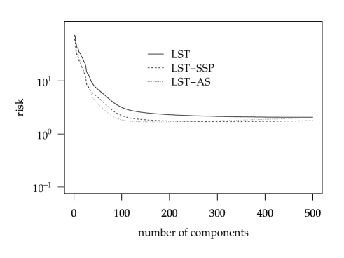
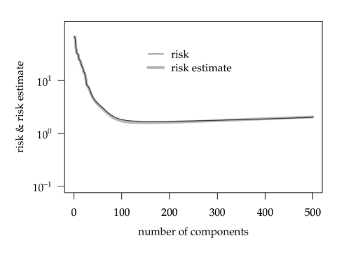
The design matrix constructed by $G_{n}$ satisfies the orthogonality condition of (2) if $x_{i}=2\pi(i-1)/n$ for $i=1,\ldots,n$ and $n$ is even. These two conditions are satisfied in our experiment here. We set $K^{*}=\{2,4,6,8\}$ and $(\beta_{2},\beta_{4},\beta_{6},\beta_{8})=(2.0,-1.5,1.0,-0.5)$, by which $h(x_{i})=\sum_{k\in K^{*}}\beta_{k}g_{k}(x_{i})$; i.e. $g_{k}$, $k\in K^{*}$ are true components. We set $\sigma^{2}=1$ for Gaussian noise variance. We also set $n=500$ and the maximum number of components that is included in a model is $50$. For an artificially generated data, we apply LST, LST-SSP(LST with single scaling parameter) and LST-AS(LST with an adaptive scaling). We employ (16) as an empirical scaling value for LST-SSP. Adaptive scaling values for LST-AS are given by (19). For each method, we calculate the approximated risk that is the mean-squared error between a true function output and estimated output on data points. We also calculate the risk estimate (unbiased estimate of risk). It is given by (12) with $\alpha=1$ for LST, (13) with $\widehat{\alpha}$ in (16) for LST-SSP and (27) with $\widehat{\alpha}_{j}$ in (19) for LST-AS. We need to estimate noise variance in calculating a risk estimate that is employed as a model selection criterion in applications. We here estimate it by the unbiased estimate of noise variance under a linear regression with a set of $250$ components that includes true components. We repeat this procedure for $1000$ times.

Figure 1: Averages of risk and risk estimate for LST-AS.

Figure 2: Averages of risk for LST, LST-SSP and LST-AS.

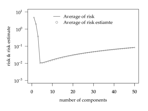
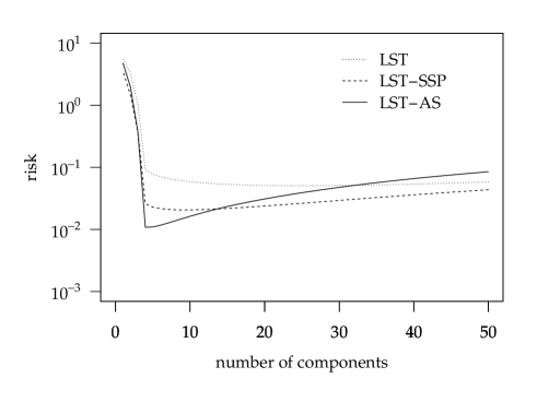
We show averages of (approximated) risks and risk estimates for LST-AS in Figure 2. We also show averages of risks for LST, LST-SSP and LST-AS in Figure 2. In Figure 2, we can see that (27) is actually valid as an unbiased risk estimate under LST-AS even when noise variance is replaced with its estimator. In Figure 2, at around a small number of components, risk of LST-AS is minimized and is smaller than those of LST and LST-SSP. However, risk of LST-AS tends to be larger than those of LST and LST-SSP as the number of components increases. This is consistent with the remark on Theorem 3 and Theorem 2. In other words, an optimal number of components can clearly be identified in risk curve of LST-AS while risk curves of LST and LST-SSP are nearly flat around the minimum value in Figure 2. We emphasize two important points in this result. The first one is that, as guaranteed by Theorem 3, risk value of LST-AS is smaller than that of LST at around an optimal number of components. The second one is that it can be found via a model selection based on risk estimate. In Table 1, we show the averaged risk value and the average numbers of un-removed components for models that are selected by risk estimates. From Table 1, we can say that LST-AS gives low risk at a sparse representation.

Table 1: Average of risk and the number of un-removed components selected according to risk estimate. The standard deviation is showed in the bracket.

method	risk	#un-removed components
LST	0.0546 (0.0186)	26.43 (12.99)
LST-SSP	0.0268 (0.0147)	16.83 (12.5)
LST-AS	0.0232 (0.0202)	10.18 (8.21)

4.2 Application to wavelet denoising

Discrete wavelet transform is a popular tool for analysis, de-noising and compression of signals and images; e.g. see [2]. We here consider an application of LST with adaptive scaling to a problem of wavelet denoising[3, 4]. Let $y(t)$ , $t\in[0,1]$ be a signal. $n$ samples of $y(t)$ is denoted by $y_{i}=y(t_{i})$, $t_{i}=(i-1)/(n-1)$, $i=1,\ldots,n$. We define ${\boldsymbol{y}}=(y_{1},\ldots,y_{n})$. We assume that $n=2^{J}$ for a natural number $J$. Let ${\boldsymbol{c}}_{j}=(c_{j,1},\ldots,c_{j,n_{j}})$ and ${\boldsymbol{d}}_{j}=(d_{j,1},\ldots,d_{j,n_{j}},\ldots,d_{J-1,1},\ldots,d_{J-1,n_{J-1}})$ be approximation and detail coefficients at a level $J$ in discrete wavelet transform, where $n_{j}=2^{j}$. We define ${\boldsymbol{w}}_{j}=({\boldsymbol{c}}_{j},{\boldsymbol{d}}_{j})$ in which we set ${\boldsymbol{w}}_{J}={\boldsymbol{c}}_{J}$ for $j=J$. By setting ${\boldsymbol{c}}_{J}={\boldsymbol{y}}$, the decomposition algorithm with pre-determined wavelets calculates ${\boldsymbol{w}}_{j-1}$ from ${\boldsymbol{c}}_{j}$ by decreasing $j=J,J-1,\ldots,J_{0}$, where $J_{0}$ is a fixed level determined by user. This procedure can be written by

$${\boldsymbol{w}}_{J_{0}}=H_{J_{0}}{\boldsymbol{y}},$$ (29)

where $H_{J_{0}}$ is an $n\times n$ orthonormal matrix that is determined by coefficients of scaling and wavelet function; e.g. see [3, 4]. On the other hand, the reconstruction algorithm calculates ${\boldsymbol{w}}_{j+1}$ from ${\boldsymbol{w}}_{j}$ by increasing $j=J_{0},\ldots,J-1,J$. This can be written by

$${\boldsymbol{w}}_{J}=H_{J_{0}}^{\prime}{\boldsymbol{w}}_{J_{0}}$$ (30)

since $H_{J_{0}}$ is an orthonormal matrix. Let $\Theta$ be an operator on $\mathbb{R}^{n}$ into $\mathbb{R}^{n}$ such as a thresholding operator. In wavelet denoising, ${\boldsymbol{w}}_{J_{0}}$ is processed by using $\Theta$ and obtain $\overline{\boldsymbol{w}}_{J_{0}}=\Theta({\boldsymbol{w}}_{J_{0}})$. We then obtain a denoised signal by $\overline{\boldsymbol{w}}_{J}=H_{J_{0}}^{\prime}\overline{\boldsymbol{w}}_{J_{0}}$. Note that, in applications, a simple and fast decomposition/reconstruction algorithm is used instead of the above matrix calculation; e.g. see [2].

We here compare the prediction accuracy and sparseness of LST-AS to those of LST, LST-SSP and also universal soft-thresholding (UST) in [3]. Note that SURE shrink of [4] is almost equivalent to LST here. In an application of UST, a threshold level on the absolute values of coefficients at the $J_{0}$th level is given by

$$\widehat{\theta}_{n}=\sqrt{2\widehat{\sigma}^{2}\log n},$$ (31)

where $\widehat{\sigma}^{2}$ is an estimate of noise variance. In wavelet denoising, the median absolute deviation (MAD) is a standard robust estimate of noise variance. It is given by

$$\widehat{\sigma}={\rm median}\{|d_{J-1,1}|,\ldots,|d_{J-1,n_{J-1}}|\}/0.6745,$$ (32)

where $d_{J-1,j}$, $j=1,\ldots,n_{J-1}$ is the smallest scale wavelet coefficients that are heuristically known to be noise dominated components. For LST, LST-SSP and LST-AS, we also employ this estimator in a model selection criterion that is an unbiased risk estimate.

We choose “heavisine” and “blocks” given in [3] as test signals. The former is almost smooth and the latter has many discontinuous points. Additive noise has a normal distribution with mean $0$ and variance $\sigma^{2}=1$. As in [3], signals are rescaled so that signal-to-noise ratio is $7$. The number of samples is $n=1024$. We set $J_{0}=2$. In [3], in practical application, it is employed a heuristic method which applies soft-thresholding only for detail coefficients at a determined level. We do not obey this heuristics and apply soft-thresholding to all coefficients in orthogonal transformation for a fair comparison. This is because the choice of a level at which thresholding applies largely depends on the performance as in [1] and there is no systematic choice of such level. We employ the orthogonal Daubechies wavelet with $8$ wavelet/scaling coefficients. For given samples, we apply LST, LST-SSP, LST-AS and UST, in which the maximum number of un-removed components is set to $300$; i.e. the maximum value of $k$ to be examined. We then calculate the mean squared error between true signal outputs and estimated outputs on the sampling points as an approximation of risk. For LST, LST-SSP and LST-AS, the mean squared error and risk estimate are obtained at each $k$. For UST, the number of un-removed components and risk value at a selected size are obtained. We repeat this procedure $500$ times.

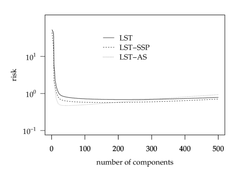
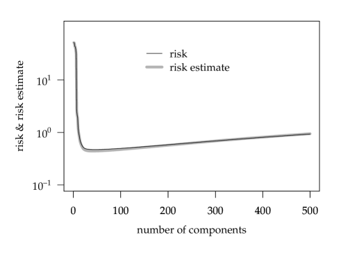
We show averages of (approximated) risk and risk estimate of LST, LST-SSP and LST-AS in Figure 3 for “heavisine” and Figure 5 for “blocks” respectively. We also show box plots of risk values at the selected number of components and those of the number of un-removed components in Figure 4 for “heavisine” and Figure 6 for “blocks” respectively. By Figure 3 (b) and Figure 5 (b), risk estimate approximates risk well for both signals even when noise variance is estimated by MAD. By Figure 3 and Figure 5, we can expect that a model estimated by LST-AS shows a low risk and high sparsity compared to LST and LST-SSP; i.e. this result leads to the same conclusions as in the previous numerical example. By comparing Figure 3 to Figure 5, the optimal number of components for “blocks” is larger than for “heavisine”, which is due to a degree of smoothness of signals. By Figure 4 and Figure 6, for both signals, LST-AS outperforms the other methods in terms of prediction accuracy and sparsity, in which especially it shows a nice sparseness property. Note that the worse results of LST and UST may be improved by applying a heuristics that thresholding methods are applied only to detail coefficients at a determined level while there is no systematic choice of the appropriate level.

(a) Averaged risk curves of LST, LST-SSP and LST-AS.

(b) Averaged risk and risk estimate of LST-AS.

Figure 3: Risk curve and risk estimate for “heavisine”.

(a) Risk value at the selected number of components.

(b) The number of un-removed components.

Figure 4: Risk and the number of un-removed components for “heavisine”.

(a) Averaged risk curve of LST, LST-SSP and LST-AS.

(b) Averaged risk curve and risk estimate of LST-AS.

Figure 5: Risk curve and risk estimate for “blocks”.

(a) Risk value at the selected number of components.

(b) The number of un-removed components.

Figure 6: Risk and the number of un-removed components for “blocks”.

5 Conclusions and future works

Soft-thresholding is a key modeling tool in statistical signal processing such as wavelet denoising. It has a parameter that simultaneously controls threshold level and amount of shrinkage. This parametrization is possible to suffer from an excess shrinkage for un-removed valid components at a sparse representation; i.e. there is a dilemma between prediction accuracy and sparsity. In this paper, to overcome this problem, we introduced a component-wise and data-dependent scaling method for soft-thresholding estimators in a context of non-parametric orthogonal regression including discrete wavelet transform. We refer this method as an adaptive scaling method. Here, we employed a LARS-based soft-thresholding method; i.e. a soft-thresholding method that is implemented by LARS under an orthogonality condition. In LARS-based soft-thresholding, a parameter value is selected by a data-dependent manner by which a model selection problem reduces to the determination of the number of un-removed components. We firstly derived a risk given by LAR-based soft-thresholding estimate with our adaptive scaling. For determining an optimal number of un-removed components, we then gave a model selection criterion as an unbiased estimate of the risk. We also analyzed some properties of the risk curve and found that the model selection criterion is possible to select a model with low risk and high sparsity compared to a naive soft-thresholding. This was verified by a simple numerical experiment and an application to wavelet denoising. As a future work, we need more application results. In doing this, estimate of noise variance should be established in general applications while MAD was found to be a good choice for a wavelet denoising application. Although we gave scaling values in a top down manner in this paper, we may need to test the other forms of adaptive scaling values; e.g. scaling values which are estimates of optimal values in some senses. Moreover, development of adaptive scaling for non-orthogonal case may be expected for more general applications.

Appendix A Lemmas

We here give some lemmas that is used for proving the main theorems.

Let $X_{1},\ldots,X_{n}$ be random variables. We define the $m$th largest value among $X_{1},\ldots,X_{n}$ by $X_{(m)}=X_{(m)}(n)$.

Lemma 1.

Let $X_{1},\ldots,X_{n}$ be i.i.d. random variables from $\chi^{2}_{1}$. We define $t_{n}=2\log n-\log\log n-\log\pi$. Then, at each fixed $k=1,2,\ldots$,

$$\lim_{n\to\infty}\mathbb{E}\left((X_{(1)}-t_{n})/2\right)^{k}=(-1)^{k}\Gamma^{(k)}(1)$$ (33)

hold, where $\Gamma^{(k)}(1)$ is the $k$th derivative of the Gamma function at $1$. (33) implies that

$$\lim_{n\to\infty}\mathbb{E}\left[X_{(1)}^{k}/t_{n}^{k}\right]=1.$$ (34)

Proof.

By slightly modifying Example 3, pp.72-73 in [14], we can show that $\mathbb{P}\left\{(X_{(1)}-t_{n})/2\leq x\right\}$ converges to the double exponential distribution. Then, (33) is a direct conclusion of Proposition 2.1 (iii) in [14]. ∎

Lemma 2.

Let $X_{1},\ldots,X_{n}$ be i.i.d. random variables from $\chi^{2}_{1}$. At each fixed $m$,

$$\lim_{n\to\infty}\mathbb{P}\left[X_{(m)}\leq 2(1-\delta)\log n)\right] =0$$ (35)

$$\lim_{n\to\infty}\mathbb{P}\left[X_{(m)}>2\log n)\right] =0$$ (36)

hold, where $\delta$ is an arbitrary positive constant.

Proof.

We denote the probability distribution function of $\chi^{2}_{1}$ by $F_{1}$. The probability density function of $\chi^{2}_{1}$ is given by $f_{1}(x)=x^{-1/2}e^{-x/2}/\sqrt{2\pi}$. We have $\frac{df_{1}(x)}{dx}=-(1/x+1)f_{1}(x)/2$. Thus, we have $\left(\int_{x}^{\infty}f_{1}(t)dt\right)/(2f_{1}(x))\to 1$ as $x\to\infty$ by applying $\int_{0}^{\infty}f_{1}(t)dt=1$ and L’Hospital’s rule. Therefore, for a $\chi_{1}^{2}$ random variable $X$,

$$\mathbb{P}[X>x]\sim 2f_{1}(x)$$ (37)

holds for a sufficiently large $x$.

By (37), we obtain

$$\mathbb{P}\left[X_{(1)}>2\log n\right] \leq\sum_{i=1}^{n}\mathbb{P}\left[X_{i}>2\log n\right]$$

$$\sim 2nf_{1}\left(2\log n\right)$$

$$=\frac{1}{\pi}\frac{1}{\sqrt{\log n}}\to 0~{}(n\to\infty).$$ (38)

Since $X_{(1)}\geq X_{(m)}$ for any $m$, we have (36). On the other hand, by (37), we have

$$n(1-F_{1}(2(1-\delta)\log n))) \sim 2nf_{1}(2(1-\delta)\log n)$$

$$\sim\frac{1}{\pi(1+\delta)}\frac{n^{\delta}}{\sqrt{\log n}}$$ (39)

for a sufficiently large $n$. Since this goes to $\infty$, we obtain (35) by Theorem 2.2.1 in [12]. ∎

Lemma 3.

For any $j\in K^{*}$ and any $\rho>0$,

$$\mathbb{P}\left[\widetilde{c}_{j}^{2}\leq\max_{i\in\overline{K}^{*}}\widetilde{c}_{i}^{2}\right]\leq 2\pi^{-1/2}\rho^{-1/2}n^{-\rho}$$ (40)

holds for a sufficiently large $n$.

Proof.

We define $\tau_{n,\rho}=2(\rho+1)\log n$. We obtain

$$\mathbb{P}\left[\widetilde{c}_{j}^{2}>\max_{i\in\overline{K}^{*}}\widetilde{c}_{i}^{2}\right] \geq\mathbb{P}\left[\left[\widetilde{c}_{j}^{2}>\tau_{n,\rho}\right]\bigcap\left[\tau_{n,\rho}>\max_{i\in\overline{K}^{*}}\widetilde{c}_{i}^{2}\right]\right]$$

$$=1-\mathbb{P}\left[\left[\widetilde{c}_{j}^{2}\leq\tau_{n,\rho}\right]\bigcup\left[\tau_{n,\rho}\leq\max_{i\in\overline{K}^{*}}\widetilde{c}_{i}^{2}\right]\right]$$

$$\geq 1-\mathbb{P}\left[\widetilde{c}_{j}^{2}\leq\tau_{n,\rho}\right]-\mathbb{P}\left[\max_{i\in\overline{K}^{*}}\widetilde{c}_{i}^{2}\geq\tau_{n,\rho}\right].$$ (41)

By the definition of $\overline{c}_{j}$, we have

$$\mathbb{P}\left[\widetilde{c}_{j}^{2}\leq\tau_{n,\rho}\right] =\mathbb{P}\left[|\widetilde{c}_{j}|\leq\sqrt{\tau_{n,\rho}}\right]$$

$$=\mathbb{P}\left[|\sqrt{n}\beta_{j}/\sigma+\overline{c}_{j}|\leq\sqrt{\tau_{n,\rho}}\right]$$

$$\leq\mathbb{P}\left[\sqrt{n}|\beta_{j}|/\sigma-|\overline{c}_{j}|\leq\sqrt{\tau_{n,\rho}}\right]$$

$$=\mathbb{P}\left[|\overline{c}_{j}|\geq\sqrt{n}|\beta_{j}|/\sigma-\sqrt{\tau_{n,\rho}}\right]$$

$$\leq\mathbb{P}\left[|\overline{c}_{j}|\geq\sqrt{\tau_{n,\rho}}\right]$$

$$=\mathbb{P}\left[\overline{c}_{j}^{2}\geq\tau_{n,\rho}\right]$$ (42)

for a sufficiently large $n$. Note that this evaluation is not tight but is enough in this paper. Since $\overline{c}_{j}^{2}\sim\chi^{2}_{1}$ by the definition of $\overline{c}_{j}$, by (37) and (A), we have

$$\mathbb{P}\left[\widetilde{c}_{j}^{2}\leq\tau_{n,\rho}\right]\leq\pi^{-1/2}\rho^{-1/2}n^{-\rho}$$ (43)

for a sufficiently large $n$.

On the other hand, $\widetilde{c}_{i}^{2}\sim\chi^{2}_{1}$ holds for $i\in\overline{K}^{*}$ since $\beta_{i}=0$ holds for $i\in\overline{K}^{*}$. By (37), we thus have

$$\mathbb{P}[\max_{i\in\overline{K}^{*}}\widetilde{c}_{i}^{2}\geq\tau_{n,\rho}] \leq\sum_{j\in\overline{K}^{*}}\mathbb{P}[\widetilde{c}_{i}^{2}\geq\tau_{n,\rho}]$$

$$\sim(n-k^{*})\pi^{-1/2}(\rho+1)^{-1/2}n^{-(\rho+1)}$$

$$\leq\pi^{-1/2}\rho^{-1/2}n^{-\rho}$$ (44)

for a sufficiently large $n$. By (A), (43) and (A), we obtain (40) as desired. ∎

Lemma 4.

$$\mathbb{P}[\overline{E}_{n}^{*}]\leq k^{*}\pi^{-1/2}\rho^{-1/2}n^{-\rho}$$ (45)

holds for any $\rho>0$ and a sufficiently large $n$.

Proof.

If $E_{n}^{*}$ does not occur then there exist $l\in\{1,\ldots,k^{*}\}$ such that $p_{l}\notin K^{*}$. This implies that there exist $j\in K^{*}$ and $i\in\overline{K}^{*}$ that satisfy $\widetilde{c}_{i}^{2}\geq\widetilde{c}_{j}^{2}$. Therefore, we have $\overline{E}_{n}^{*}\subseteq\bigcup_{j\in K^{*}}F_{j}$. By Lemma 3, we then obtain (45). ∎

Lemma 5.

$$\lim_{n\to\infty}\mathbb{E}\widetilde{c}_{p_{1}}^{2m}I_{\overline{E}_{n}^{*}}=0$$ (46)

holds for a fixed $m=1,2,\cdots$.

Proof.

We define $\overline{c}=\max_{1\leq i\leq n}|\overline{c}_{i}|$ and $\overline{\beta}=\max_{j\in K^{*}}|\beta_{j}|$. We also define an event $F=\left\{\overline{c}>(\overline{\beta}/\sigma)\sqrt{n}\right\}$. By the Cauchy-Schwarz inequality, we have

$$\mathbb{E}[\widetilde{c}_{p_{1}}^{2m}I_{\overline{E}_{n}^{*}}]$$

$$\leq\mathbb{E}[(\overline{c}_{p_{1}}+(\beta_{p_{1}}/\sigma)\sqrt{n})^{2m}I_{\overline{E}_{n}^{*}}]$$

$$\leq\mathbb{E}[(\overline{c}+(\overline{\beta}/\sigma)\sqrt{n})^{2m}I_{\overline{E}_{n}^{*}}]$$

$$\leq\mathbb{E}[(\overline{c}+(\overline{\beta}/\sigma)\sqrt{n})^{2m}I_{F}I_{\overline{E}_{n}^{*}}]+\mathbb{E}[(\overline{c}+(\overline{\beta}/\sigma)\sqrt{n})^{2m}I_{\overline{F}}I_{\overline{E}_{n}^{*}}]$$

$$\leq 2^{2m}\mathbb{E}[\overline{c}^{2m}I_{F}I_{\overline{E}_{n}^{*}}]+2^{2m}(\overline{\beta}/\sigma)^{2m}n^{m}\mathbb{E}[I_{\overline{F}}I_{\overline{E}_{n}^{*}}]$$

$$\leq 2^{2m}\mathbb{E}[(\overline{c}^{2})^{m}I_{\overline{E}_{n}^{*}}]+2^{2m}(\overline{\beta}/\sigma)^{2m}n^{m}\mathbb{E}[I_{\overline{E}_{n}^{*}}]$$

$$\leq 2^{2m}\sqrt{\mathbb{E}[(\overline{c}^{2})^{2m}]}\sqrt{\mathbb{P}[\overline{E}_{n}^{*}]}+2^{2m}(\overline{\beta}/\sigma)^{2m}n^{m}\mathbb{P}[\overline{E}_{n}^{*}].$$ (47)

By Lemma 4 with $\rho>m$, the second term of (A) goes to zero as $n\to\infty$. Since $\overline{c}^{2}$ is the largest value among i.i.d. $\chi^{2}_{1}$ sequence with size $n$, the first term of (A) goes to zero as $n\to\infty$ by Lemma 1 and Lemma 4 with the above choice of $\rho$. ∎

Lemma 6.

If $k\geq k^{*}$ then

$$\mathbb{E}[\widetilde{\theta}_{k}^{2m}]\leq(2\log n)^{m}$$ (48)

holds for a fixed $m=1,2,\cdots$ and sufficiently large $n$.

Proof.

We can write

$$\mathbb{E}\left[\widetilde{\theta}_{k}^{2m}\right]=\mathbb{E}\left[\widetilde{\theta}_{k}^{2m}I_{\overline{E}_{n}^{*}}\right]+\mathbb{E}\left[\widetilde{\theta}_{k}^{2m}I_{E_{n}^{*}}\right].$$ (49)

By Lemma 5 and the definition of $\widetilde{\theta}_{k}$,

$$\mathbb{E}\left[\widetilde{\theta}_{k}^{2}I_{\overline{E}_{n}^{*}}\right]\leq\mathbb{E}\left[\widetilde{c}_{p_{1}}^{2m}I_{\overline{E}_{n}^{*}}\right]\to 0~{}(n\to\infty).$$ (50)

We define $\widetilde{c}^{2}=\max_{i\in\overline{K}^{*}}\widetilde{c}_{i}^{2}$. If $E_{n}^{*}$ occurs then $\widetilde{\theta}_{k}^{2}\leq\widetilde{c}^{2}$ and $\widetilde{c}^{2}$ is the largest value among i.i.d. $\chi_{1}^{2}$ random sequence with length $(n-k^{*})$. Therefore, by Lemma 1,

$$\frac{\mathbb{E}\left[\widetilde{\theta}_{k}^{2m}I_{E_{n}^{*}}\right]}{(2\log n)^{m}}\leq\frac{\mathbb{E}\left[\widetilde{c}^{2m}\right]}{(2\log n)^{m}}\to 1~{}(n\to\infty).$$ (51)

∎

Appendix B Proof of Theorems

We give the proofs of the main theorems below.

Proof of Theorem 1.

For an ${\widehat{\boldsymbol{\alpha}}}$, the risk is reformulated as

$$R_{\rm AS}(n,k) =\mathbb{E}\|\widehat{\bf{A}}\widehat{\boldsymbol{b}}_{k}-{\boldsymbol{\beta}}\|^{2}$$

$$=\mathbb{E}\|\widehat{\bf{A}}\widehat{\boldsymbol{b}}_{k}-\widehat{\boldsymbol{c}}\|^{2}+\mathbb{E}\|\widehat{\boldsymbol{c}}-{\boldsymbol{h}}\|^{2}+2\mathbb{E}(\widehat{\bf{A}}\widehat{\boldsymbol{b}}_{k}-\widehat{\boldsymbol{c}})^{\prime}(\widehat{\boldsymbol{c}}-{\boldsymbol{\beta}})$$

$$=\mathbb{E}\|\widehat{\bf{A}}\widehat{\boldsymbol{b}}-\widehat{\boldsymbol{c}}\|^{2}+\sigma^{2}+2\mathbb{E}(\widehat{\bf{A}}\widehat{\boldsymbol{b}}_{k}-\widehat{\boldsymbol{c}})^{\prime}(\widehat{\boldsymbol{c}}-{\boldsymbol{\beta}})$$

$$=\frac{1}{n}\mathbb{E}\|\widehat{\boldsymbol{\mu}}_{k,\alpha}-{\boldsymbol{y}}\|^{2}+\sigma^{2}+2\mathbb{E}(\widehat{\bf{A}}\widehat{\boldsymbol{b}}_{k}-\widehat{\boldsymbol{c}})^{\prime}(\widehat{\boldsymbol{c}}-{\boldsymbol{\beta}})$$

$$=\frac{1}{n}\mathbb{E}\|\widehat{\boldsymbol{\mu}}_{k,\alpha}-{\boldsymbol{y}}\|^{2}+\sigma^{2}+\frac{2\sigma^{2}}{n}\mathbb{E}(\widehat{\bf{A}}\widetilde{\boldsymbol{b}}_{k}-\widetilde{\boldsymbol{c}})^{\prime}(\widetilde{\boldsymbol{c}}-{\boldsymbol{c}}),$$ (52)

where we used (4) at the third line and the orthogonality condition at the last line. The last term is often called the degree of freedom; see e.g. [5].

Let $\widetilde{\boldsymbol{c}}_{-j}$ be an $n-1$-dimensional vector that is constructed by removing $\widetilde{c}_{j}$ from $\widetilde{\boldsymbol{c}}$. We define $d_{j}(\widetilde{\boldsymbol{c}})=(\widehat{\alpha}_{j}\widetilde{b}_{k,j}-\widetilde{c}_{j})$. Although $d_{j}$ is a function of $\widetilde{\boldsymbol{c}}$, we regard this as a function $\widetilde{c}_{j}$ under a fixed $\widetilde{\boldsymbol{c}}_{-j}$ and denote it by $d_{j}(\widetilde{c}_{j}|\widetilde{\boldsymbol{c}}_{-j})$. Let $\theta_{j}$ be the $k$th largest value in $\{|\widetilde{c}_{i}|:i=1,\ldots,n,i\neq j\}$. By (19), we have

$$d_{j}(\widetilde{c}_{j}|\widetilde{\boldsymbol{c}}_{-j})=\widehat{\alpha}_{j}\widetilde{b}_{k,j}-\widetilde{c}_{j}=\begin{cases}-\theta_{j}^{2}/\widetilde{c}_{j}&|\widetilde{c}_{j}|>\theta_{j}\\ -\widetilde{c}_{j}&|\widetilde{c}_{j}|\leq\theta_{j}\\ \end{cases}.$$ (53)

Note here that $d_{j}(\widetilde{c}_{j}|\widetilde{\boldsymbol{c}}_{-j})$ is well-defined even when $\widetilde{c}_{j}=0$ under the definition of $\widehat{\alpha}_{j}$ in (19). This is Lipschitz continuous as a function of $\widetilde{c}_{j}$ when $\widetilde{\boldsymbol{c}}_{-j}$ is fixed. It is thus absolutely continuous. On the other hand, we denote expectation with respect to $\widetilde{\boldsymbol{c}}$ by $\mathbb{E}_{\widetilde{\boldsymbol{c}}}$. We have $\widetilde{\boldsymbol{c}}={\bf{G}}^{\prime}{\boldsymbol{y}}/(\sigma\sqrt{n})$ and $|{\rm det}({\bf{G}}^{\prime}{\boldsymbol{y}}/(\sigma\sqrt{n}))^{-1})|=\sigma^{n}$, where ${\rm det}$ denotes the determinant of a matrix. Therefore, $\mathbb{E}$ is always replaced with $\mathbb{E}_{\widetilde{\boldsymbol{c}}}$ by change of variables. We also denote a conditional expectation with respect to $\widetilde{c}_{j}$ given $\widetilde{\boldsymbol{c}}_{-j}$ by $\mathbb{E}_{\widetilde{c}_{j}|\widetilde{\boldsymbol{c}}_{-j}}$. We define $I_{[-\theta_{j},\theta_{j}]}(\widetilde{c}_{j}|\widetilde{\boldsymbol{c}}_{-j})$ by $I_{[-\theta_{j},\theta_{j}]}(\widetilde{c}_{j}|\widetilde{\boldsymbol{c}}_{-j})=1$ when $\widetilde{c}_{j}\in[-\theta_{j},\theta_{j}]$ and $0$ otherwise under a fixed $\widetilde{\boldsymbol{c}}_{-j}$. Then, by applying this change of variables and Stein’s lemma[15] under the above absolutely continuity, we obtain

$$\mathbb{E}(\widehat{\bf{A}}\widetilde{\boldsymbol{b}}_{k}-\widetilde{\boldsymbol{c}})^{\prime}(\widetilde{\boldsymbol{c}}-{\boldsymbol{c}})$$

$$=\sum_{j=1}^{n}\mathbb{E}\left[d_{j}(\widetilde{\boldsymbol{c}})(\widetilde{c}_{j}-c_{j})\right]$$

$$=\sum_{j=1}^{n}\mathbb{E}_{\widetilde{\boldsymbol{c}}}\left[d_{j}(\widetilde{\boldsymbol{c}})(\widetilde{c}_{j}-c_{j})\right]$$

$$=\sum_{j=1}^{n}\mathbb{E}_{\widetilde{\boldsymbol{c}}_{-j}}\mathbb{E}_{\widetilde{c}_{j}|\widetilde{\boldsymbol{c}}_{-j}}\left[d_{j}(\widetilde{c}_{j}|\widetilde{\boldsymbol{c}}_{-j})(\widetilde{c}_{j}-c_{j})\right]$$

$$=\sum_{j=1}^{n}\mathbb{E}_{\widetilde{\boldsymbol{c}}_{-j}}\mathbb{E}_{\widetilde{c}_{j}|\widetilde{\boldsymbol{c}}_{-j}}\left[\frac{\partial d_{j}(\widetilde{c}_{j}|\widetilde{\boldsymbol{c}}_{-j})}{\partial\widetilde{c}_{j}}\right]$$

$$=\mathbb{E}_{\widetilde{\boldsymbol{c}}}\left[\sum_{j=1}^{n}(\theta_{j}^{2}/\widetilde{c}_{j}^{2})(1-I_{[-\theta_{j},\theta_{j}]}(\widetilde{c}_{j}|\widetilde{\boldsymbol{c}}_{-j}))\right]-\mathbb{E}_{\widetilde{\boldsymbol{c}}}\left[\sum_{j=1}^{n}I_{[-\theta_{j},\theta_{j}]}(\widetilde{c}_{j}|\widetilde{\boldsymbol{c}}_{-j})\right]$$

$$=\mathbb{E}\left[\sum_{j\in\widehat{K}_{k}}(\widehat{\alpha}_{j}-1)^{2}\right]-(n-k),$$ (54)

where the last line is obtained by the definition of $\theta_{j}$ and $\widehat{\alpha}_{j}$. (B) and (B) yield (21). ∎

Proof of Theorem 2.

We show that

$$\mathbb{P}\left[\widehat{\alpha}_{j}>1+\epsilon_{j,n}\right]\to 0~{}(n\to\infty)$$ (55)

for $j\in K^{*}$. We define $E_{0}=\{\widetilde{c}_{j}=0\}$ for which $\mathbb{P}[E_{0}]=0$. By the definition of $\widehat{\alpha}_{j}$ in (19), we then have

$$\mathbb{P}\left[\widehat{\alpha}_{j}>1+\epsilon_{j,n}\right]$$

$$=\mathbb{P}\left[\left\{\widehat{\alpha}_{j}>1+\epsilon_{j,n}\right\}\bigcap\overline{E}_{0}\right]$$

$$=\mathbb{P}\left[\left\{\frac{\widetilde{\theta}_{k}}{|\widetilde{c}_{j}|}>\epsilon_{j,n}\right\}\bigcap\overline{E}_{0}\right]$$

$$\leq\mathbb{P}\left[\frac{\widetilde{\theta}_{k}}{\sqrt{2\log n}}-\frac{|\widetilde{c}_{j}|}{(|\beta_{j}|+\delta)\sqrt{n}}>0\right]$$

$$\leq\mathbb{P}\left[\widetilde{\theta}_{k}>\sqrt{2\log n}\right]+\mathbb{P}\left[|\widetilde{c}_{j}|<(|\beta_{j}|+\delta)\sqrt{n}\right].$$ (56)

For the first term of (B), we have

$$\mathbb{P}\left[\widetilde{\theta}_{k}>\sqrt{2\log n}\right]$$

$$=\mathbb{P}\left[\widetilde{\theta}_{k}^{2}>2\log n\right]$$

$$=\mathbb{P}\left[\widetilde{\theta}_{k}^{2}>2\log n|E_{n}^{*}\right]\mathbb{P}\left[E_{n}^{*}\right]+\mathbb{P}\left[\widetilde{\theta}_{k}^{2}>2\log n|\overline{E}_{n}^{*}\right]\mathbb{P}\left[\overline{E}_{n}^{*}\right]$$

$$\leq\mathbb{P}\left[\widetilde{\theta}_{k}^{2}>2\log n|E_{n}^{*}\right]+\mathbb{P}\left[\overline{E}_{n}^{*}\right].$$ (57)

The second term of (B) goes to zero as $n\to\infty$ by Lemma 4. If $E_{n}^{*}$ occurs then $\widetilde{\theta}_{k}^{2}$ is the $(k+1-k^{*})$th largest value among i.i.d. $\chi_{1}^{2}$ random sequence with size $n-k^{*}$. Therefore, by (36) in Lemma 2, the first term of (B) goes to zero as $n\to\infty$. Thus, the first term of (B) goes to zero as $n\to\infty$. Recall that $\widetilde{c}_{j}=\sqrt{n}\beta_{j}+\overline{c}_{j}$ for $j\in K^{*}$, where $\overline{c}_{j}\sim N(0,1)$. Then, for the second term of (B), we obtain

$$\mathbb{P}\left[|\widetilde{c}_{j}|<(|\beta_{j}|+\delta)\sqrt{n}\right] =\mathbb{P}\left[|\sqrt{n}\beta_{j}+\overline{c}_{j}|<(|\beta_{j}|+\delta)\sqrt{n}\right]$$

$$\leq\mathbb{P}\left[\sqrt{n}|\beta_{j}|-|\overline{c}_{j}|<(|\beta_{j}|+\delta)\sqrt{n}\right]$$

$$=\mathbb{P}\left[|\overline{c}_{j}|>\delta\sqrt{n}\right]\to 0~{}(n\to\infty).$$ (58)

Since $\widehat{\alpha}_{j}\geq 1$ holds, we obtain (23) as desired.

On the other hand, we consider (25). For any $\delta_{n}$, we have

$$\mathbb{P}\left[\widehat{\alpha}_{j}\leq 2-\epsilon\right] =\mathbb{P}\left[\{\widehat{\alpha}_{j}\leq 2-\epsilon\}\bigcap\overline{E}_{0}\right]$$

$$\leq\mathbb{P}\left[\widetilde{\theta}_{k}\leq(1-\epsilon)|\widetilde{c}_{j}|\right]$$

$$\leq\mathbb{P}\left[\widetilde{\theta}_{k}\leq\delta_{n}\right]+\mathbb{P}\left[(1-\epsilon)|\widetilde{c}_{j}|>\delta_{n}\right].$$ (59)

For the first term of (B), we have

$$\mathbb{P}\left[\widetilde{\theta}_{k}\leq\delta_{n}\right] =\mathbb{P}\left[\widetilde{\theta}_{k}^{2}\leq\delta_{n}^{2}\right]$$

$$=\mathbb{P}\left[\widetilde{\theta}_{k}^{2}\leq\delta_{n}^{2}|E_{n}^{*}\right]\mathbb{P}[E_{n}^{*}]+\mathbb{P}\left[\widetilde{\theta}_{k}\leq\delta_{n}^{2}|\overline{E}_{n}^{*}\right]\mathbb{P}[\overline{E}_{n}^{*}]$$

$$\leq\mathbb{P}\left[\widetilde{\theta}_{k}^{2}\leq\delta_{n}^{2}|E_{n}^{*}\right]+\mathbb{P}[\overline{E}_{n}^{*}].$$ (60)

By Lemma 4, the second term of (B) goes to zero as $n\to\infty$. We set $\delta_{n}=\sqrt{2(1-\epsilon)\log n}$. If $E_{n}^{*}$ occurs then $\widetilde{\theta}_{k}^{2}$ is the $(k+1-k^{*})$th largest value among i.i.d. $\chi_{1}^{2}$ random sequence with size $n-k^{*}$. Therefore, by (35) in Lemma 2 and the choice of $\delta_{n}$, the first term of (B) goes to zero as $n\to\infty$. We define $\widetilde{c}^{2}=\max_{i\in\overline{K}^{*}}\widetilde{c}_{i}^{2}$. For the second term of (B), we have

$$\mathbb{P}\left[(1-\epsilon)|\widetilde{c}_{j}|>\delta_{n}\right]\leq\mathbb{P}\left[\widetilde{c}^{2}>2\log n\right]$$ (61)

since $j\in K^{*}$. Here, $\widetilde{c}^{2}$ is the largest value among i.i.d. $\chi_{1}^{2}$ random sequence with size $n-k^{*}$ by the definitions of $\widetilde{c}_{i}$ and $K^{*}$. Hence, by (36) in Lemma 2, (61) goes to zero as $n\to\infty$. ∎

Proof of Theorem 3.

By (12) and (21), we have

$$R_{n,k^{*}}({\bf{1}}_{n})-R_{\rm AS}(n,k^{*})$$

$$=\frac{\sigma^{2}}{n}\sum_{j=1}^{k^{*}}\left(\mathbb{E}\left[(\widehat{\alpha}_{p_{j}}-1)^{2}\widetilde{c}_{p_{j}}^{2}\right]-\mathbb{E}\left[(\widehat{\alpha}_{p_{j}}-1)^{2}\widetilde{\theta}_{k^{*}}^{2}\right]-2\mathbb{E}\left[(\widehat{\alpha}_{p_{j}}-1)^{2}\right]\right)$$

$$=\frac{\sigma^{2}2\log n}{n}\sum_{j=1}^{k^{*}}\left(\frac{\mathbb{E}\left[\widetilde{\theta}_{k^{*}}^{2}\right]}{2\log n}-\frac{\mathbb{E}\left[(\widehat{\alpha}_{p_{j}}-1)^{2}\widetilde{\theta}_{k^{*}}^{2}\right]}{2\log n}-2\frac{\mathbb{E}\left[(\widehat{\alpha}_{p_{j}}-1)^{2}\right]}{2\log n}\right)$$ (62)

through a simple calculation. We evaluate the three terms in the sum of (B). We first have

$$\lim_{n\to\infty}\mathbb{E}[\widetilde{\theta}_{k^{*}}^{2}]/(2\log n)=1$$ (63)

by Lemma 6. Hence, the proof is completed by showing that the second and third terms of (B) goes to zero as $n\to\infty$. We define $\epsilon_{n}=\max_{j\in K^{*}}\epsilon_{j,n}$ and $G_{j}=\{(\widehat{\alpha}_{p_{j}}-1)^{2}>\epsilon_{n}^{2}\}$, where $\epsilon_{j,n}$ is defined in (22). We have $(\widehat{\alpha}_{p_{j}}-1)^{2}\leq 1$ for $j\leq k^{*}$ by the definition of $\widetilde{\theta}_{k^{*}}=|\widetilde{c}_{p_{k^{*}+1}}|$. And, if $E_{n}^{*}$ occurs then $\bigcup_{l\in K^{*}}\{p_{j}=l\}$ for any $j\in\{1,\ldots,k^{*}\}$. We then obtain

$$\mathbb{E}\left[(\widehat{\alpha}_{p_{j}}-1)^{2}\right] =\mathbb{E}\left[(\widehat{\alpha}_{p_{j}}-1)^{2}I_{G_{j}\bigcap E_{n}^{*}}\right]+\mathbb{E}\left[(\widehat{\alpha}_{p_{j}}-1)^{2}I_{\overline{G}_{j}\bigcup\overline{E}_{n}^{*}}\right]$$

$$\leq\mathbb{E}\left[I_{G_{j}\bigcap\overline{E}_{n}^{*}}\right]+\epsilon_{n}^{2}+\mathbb{P}[\overline{E}_{n}^{*}]$$

$$\leq\sum_{l\in K^{*}}\mathbb{P}\left[(\widehat{\alpha}_{l}-1)^{2}>\epsilon_{n}^{2}\right]+\epsilon_{n}^{2}+\mathbb{P}[\overline{E}_{n}^{*}].$$ (64)

(B) goes to zero as $n\to\infty$ by (23) in Theorem 2, the definition of $\epsilon_{n}$ and Lemma 4. We also have

$$\mathbb{E}\left[(\widehat{\alpha}_{p_{j}}-1)^{2}\widetilde{\theta}_{k^{*}}^{2}\right]$$

$$=\mathbb{E}\left[(\widehat{\alpha}_{p_{j}}-1)^{2}\widetilde{\theta}_{k^{*}}^{2}I_{G_{j}\bigcap E_{n}^{*}}\right]+\mathbb{E}\left[(\widehat{\alpha}_{p_{j}}-1)^{2}\widetilde{\theta}_{k^{*}}^{2}I_{\overline{G}_{j}\bigcup\overline{E}_{n}^{*}}\right]$$

$$\leq\mathbb{E}\left[\widetilde{\theta}_{k^{*}}^{2}I_{G_{j}}I_{E_{n}^{*}}\right]+\epsilon_{n}^{2}\mathbb{E}[\widetilde{\theta}_{k^{*}}^{2}]+\mathbb{E}[\widetilde{\theta}_{k^{*}}^{2}I_{\overline{E}_{n}^{*}}].$$ (65)

For the first term of (B), by the Cauchy-Schwarz inequality, we have

$$\frac{\mathbb{E}\left[\widetilde{\theta}_{k^{*}}^{2}I_{G_{j}}I_{E_{n}^{*}}\right]}{2\log n} \leq\frac{\sqrt{\mathbb{E}\left[\widetilde{\theta}_{k^{*}}^{4}\right]}}{2\log n}\sqrt{\mathbb{E}\left[I_{G_{j}}I_{E_{n}^{*}}\right]}$$

$$\leq\frac{\sqrt{\mathbb{E}\left[\widetilde{\theta}_{k^{*}}^{4}\right]}}{2\log n}\sqrt{\sum_{l\in K^{*}}\mathbb{P}\left[(\widehat{\alpha}_{l}-1)^{2}>\epsilon_{n}^{2}\right]}.$$ (66)

(B) goes to zero as $n\to\infty$ by Lemma 6 and (23) in Theorem 2. The second term of (B) goes to zero as $n\to\infty$ by Lemma 6 and the definition of $\epsilon_{n}$. By the Cauchy-Schwarz inequality, the third term of (B) is bounded above by $\sqrt{\mathbb{E}[\widetilde{\theta}_{k^{*}}^{4}]}\sqrt{\mathbb{P}[\overline{E}_{n}^{*}]}$. This goes to zero as $n\to\infty$ by Lemma 6 and Lemma 4. We thus obtain (26) as desired. ∎

References

- Abramovich and Yoav [1996] Abramovich, F., B. Yoav, 1996. Adaptive thresholding of wavelet coefficients. Computational Statistics & Data Analysis 22, 351-361.
- Burrus et al. [1998] Burrus, C.S., Gopinath, R.A., Guo, H., 1998. Introduction to wavelets and wavelet transform. Prentice Hall.
- Donoho and Johnstone [1994] Donoho, D.L., Johnstone, I.M., 1994. Ideal spatial adaptation via wavelet shrinkage. Biometrika 81, 425-455.
- Donoho and Johnstone [1995] Donoho, D.L., Johnstone, I.M., 1995. Adapting to unknown smoothness via wavelet shrinkage. J. Amer. Statist. Assoc. 90, 1200-1224.
- Efron et al. [2004] Efron, B., Hastie, T., Johnstone, I., Tibshirani, R., 2004. Least angle regression. Ann. Stat. 32, 407-499.
- Fan and Li [2001] Fan, J. and Li, R., 2001. Variable selection via nonconcave penalized likelihood and its oracle properties. J. Amer. Statist. Assoc. 96, 1348-1360.
- Hagiwara [2006] Hagiwara, K., 2006. On the expected prediction error of orthogonal regression with variable components. IEICE Trans. Fundamentals E89-A, 3699-3709.
- Hagiwara [2014] Hagiwara, K., 2014. Least angle regression in orthogonal case, in: Proceedings of ICONIP 2014, Part II, LNCS 8835, Springer, 540-547.
- Hagiwara [2015] Hagiwara, K., 2015. On scaling of soft-thresholding estimator, Submitted to Neurocomputing.
- Hurvich and Tsai [1998] Hurvich C.M. and Tsai C. 1998. A crossvalidatory AIC for hard wavelet thresholding in spatially adaptive function estimation. Biometrika 85, 701-710.
- Knight and Fu [2000] Knight, K., Fu, W., 2000. Asymptotics for lasso-type estimators. Ann. Stat. 28, 1356-1378.
- Leadbetter et al. [1983] Leadbetter, M.R., Lindgren, G., Rootzén, H., 1983. Extremes, and related properties of random sequences and processes. Springer-Verlag.
- Nason [1996] Nason, G.P., 1996. Wavelet shrinkage using cross-validation. J. R. Statist. Soc. B 58, 463-79.
- Resnick [1987] Resnick, S.I., 1987. Extreme values, regular variation, and point processes. Springer-Verlag.
- Stein [1981] Stein, C., 1981. Estimation of the mean of a multivariate normal distribution. Ann. Stat. 9, 1135-1151.
- Tibshirani [1996] Tibshirani, R., 1996. Regression shrinkage and selection via the lasso. J. R. Stat. Soc. Ser. B Stat. Methodol. 58, 267-288.
- Zhao and Yu [2006] Zhao, P., Yu, B., 2006. On model selection consistency of Lasso. J. Mach. Learn. Res. 7, 2541-2563.
- Zou [2006] Zou, H., 2006. The adaptive lasso and its oracle properties. J. Amer. Statist. Assoc. 101, 1418-1492.
- Zou et al. [2007] Zou, H., Hastie, T., Tibshirani, R., 2007. On the degrees of freedom of LASSO. Ann. Stat. 35, 2173-2192.
- Zou and Hastie [2005] Zou, H., Hastie, T., 2005. Regularization and variable selection via the elastic net. J. R. Stat. Soc. Ser. B Stat. Methodol. 67, 301-320.